Recovery guarantees for multifrequency chirp waveforms in compressed radar sensing

Abstract

Radar imaging systems transmit modulated wideband waveform to achieve high range resolution resulting in high sampling rates at the receiver proportional to the bandwidth of the transmit waveform. Analog processing techniques can be used on receive to reduce the number of measurements to $N$, the number of potential delay bins. If the scene interrogated by the radar is assumed to be sparse consisting of $K$ point targets, results from compressive sensing suggest that number of measurements can be further reduced to scale with $K\log N$ for stable recovery of a sparse scene from measurements with additive noise. While unstructured random projectors guarantee successful recovery under sparsity constraints, they cannot be implemented in the radar hardware in practice. Recently, structured random Toeplitz and Circulant matrices that result from using stochastic waveforms in time delay estimation setting have been shown to yield recovery guarantees similar to unstructured sensing matrices. However, the corresponding transmitter and receiver structures have high complexity and large storage requirements. In this paper, we propose an alternative low complexity compressive wideband radar sensor which combines multitone signal chirp waveform on transmit with a receiver that utilizes an analog mixer followed with a uniform sub-Nyquist sampling stage. We derive the recovery guarantees for the resulting structured measurement matrix and sufficient conditions for the number of tones. The only random component of our design is the sparse tone spectrum implementable efficiently in hardware. Our analytical and empirical results show that the performance of our scheme is in par with unstructured random sensing matrices and structured Toeplitz and Circulant matrices with random entries.

I Introduction

Radar imaging systems acquire information about the scene of interest by transmitting pulsed waveforms and analyze the received backscatter energy to form an estimate of the range and amplitude of the reflectors in the scene. These range profiles from multiple pulses and/or multiple antenna elements can be processed jointly to solve a multitude of inference tasks including detection, tracking and classification [1]. In this paper, we focus on the problem of estimation of range and amplitude of reflectors in the scene using a single modulated wideband pulse $\phi(t)$ of bandwidth $B$. The resolution of the echo imaging system is directly proportional to the bandwidth of the transmitted signal. Assuming the support of the observed delays are known to lie on an interval $T$ (termed as range swath in radar literature), then the unknown range profile can be discretized into $N=BT$ delay bins. The signal model at the receiver can be written as $y(t)=\sum_{n=1}^{N}x_{n}\phi(t-n\Delta)+n(t)$, where $\Delta=1/B$, $n(t)$ is the receiver noise and $x_{n}$ denotes the complex scattering coefficients associated with the $n^{\prime}$th delay bin. Commonly the received signal is matched filtered with a copy of the transmitted pulse to detect reflectors in range and estimate their complex amplitude of backscattered energy. Direct digital implementation of the matched filtering step requires quadrature sampling of the received signal for the pulse duration with sampling rate matching the bandwidth of the transmit waveform. Alternatively, the matched filtering can be implemented in the analog domain where the number of samples are reduced to $N$ to cover the delay support. However, the match filter output still requires to be sampled at the Nyquist rate corresponding to the system bandwidth, rendering digital and analog matched filter receivers for arbitrary waveforms impractical for bandwidths exceeding gigahertz for current analog to digital converter (ADC) technology.

If a linear frequency modulated waveform (LFM) $\phi(t)=e^{j\beta t^{2}}$ is used on transmit, the matched filtering can be approximately implemented through mixing the received signal with a reference LFM waveform and low pass filtering the mixer output. At the mixer output each copy of the waveform delayed by $\Delta$ appears as a tone whose frequency is given by $\beta\Delta$. This pre-processing step is termed stretch processing [1, 2] and can result in substantially reduced sampling rate for the ADC used in the mixer output if the delay support $T$ is smaller than the pulse length. Specifically, received signal at stretch processor’s output can be written as:

$$y(t)=\sum_{n=1}^{N}x_{n}e^{j(n\beta\Delta)t},$$ (1)

In essence, stretch processing converts range profile estimation problem into frequency spectrum estimation problem with Nyquist rate samples in time obtained after analog processing. If the scene can be assumed to have fewer targets $K$ than the number of delay bins $N$, well-known results [3, 4] from the Compressive sensing (CS) shows successful reconstruction with sub-Nyquist samples is possible with the number of measurements $M$ scaling with $K\log N$, if appropriate measurement operators can be implemented. Furthermore, there are numerous tractable algorithms with provable performance that are either based on convex relaxation [5, 6, 7] or greedy methods [8, 9] to solve the reconstruction problem. Motivated by these advances, compressed sensing techniques have been applied to a variety of problems in Radar [10]: range profile estimation [11], single pulse systems for range-doppler estimation in [12], single pulse multiple transmit and receive system for range-doppler and azimuth estimation and target detection in [13, 14], remote sensing in [15], direction of arrival estimation in [16]. CS based radar sensors based on pure random waveforms [17], Xampling framework [18] and Random Modulator Pre-Integrator (RMPI) framework [19] using the receiver structure from [20] have also been implemented. A common theme in most of the CS literature has been randomization as it leads to measurement matrices that have provable recovery guarantees. Implementation of the randomness into compressive radar systems has proven to be a challenging task in practice; uncorrelated random signals with high peak-to-average power ratio is mismatched to the nonlinear power amplifiers used in radar systems and the system bandwidth (and as a result range resolution) is limited as digital to analog converters (DAC) have to be employed for generation of precise random signals for transmit and receive mixing.

The LFM pulse model in (1) provides an alternative strategy as it converts the range estimation problem into an equivalent sparse frequency spectrum estimation problem. Uniform subsampling in this setting has poor perforamnce [21]. Non-uniform random sub-sampling can be used to obtain measurements with low mutual coherency [22, 21]. However, non-uniform sampling with commercially available ADCs still requires it to be rated at the Nyquist rate to accommodate closely spaced samples. We propose to use low speed uniform sub-sampling using a high analog bandwidth ADC in the sparse frequency spectrum estimation setting and push randomness to transmit signal structure to obtain compressive measurements. ADCs whose analog bandwidth exceeds their maximum sampling rate by several factors is readily available and used routinely in pass-band sampling. This compressive radar structure proposed in [23] uses linear combination of LFM waveform at the transmitter with randomly selected center frequencies, while maintaining the simple standard stretch processing receiver structure. The output of the stretch processor receiver is given by

$$y(t)=\sum_{n=1}^{N}x_{n}\sum_{k=1}^{N_{c}}e^{j\phi_{n,k}}e^{j\left({n\beta\Delta+\omega_{k}}\right)t}$$

where $\phi_{n,k}$ is a predetermined known complex phase, $N_{c}$ is the number of tones modulating the LFM waveform. We observe that under the proposed compressive sensor design each delayed copy of the transmitted waveform is mapped to multi-tone spectra with known structure. As shown in this paper this known multi-tone frequency structure enables recovery from aliased time samples with provable guarantees. These results complement previous work which has shown good empirical performance in simulation and measurements [24].

The contributions put forth in this sequel is that we present the theoretical analysis for this multi-frequency LFM system. We show that the system with a relatively small number of LFM waveform has performance guarantees similar to a matrix with independent random entries for a sufficiently large number of tones modulating the LFM waveform. We also present a numerical analysis comparing our system with other measurement schemes.

Notation and Preliminaries

We denote a vector in $N$-dimensional complex domain as $\mathbf{x}\in\mathbb{C}^{N}$. $\left\lVert{\mathbf{x}}\right\rVert_{0}$ is called as $\ell_{0}$ norm, which is given as the number of non-zero elements in a vector. Clearly, this is not a valid norm but is used in formulating the fundamental problem in compressed sensing. We denote $\left\lVert{\mathbf{x}}\right\rVert_{1}=\sum_{i}\left\lvert{x_{i}}\right\rvert$ as the $\ell_{1}$ norm. The Euclidean or $\ell_{2}$ norm is given as $\left\lVert{\mathbf{x}}\right\rVert_{2}=\sqrt{\sum_{i}\left\lvert{x_{i}}\right\rvert^{2}}$. We denote a matrix as $\mathbf{A}\in\mathbb{C}^{M\times N}$, $\mathbf{A}^{*}\in\mathbb{C}^{N\times M}$ as conjugate transpose of $\mathbf{A}$, and $\mathbf{I}$ as the identity matrix of dimensions dependent on the context. The spectral or operator norm of the matrix is given as $\left\lVert{\mathbf{A}}\right\rVert_{op}=\sigma_{\max}(\mathbf{A})$ the largest singular value of the matrix. The Frobenius norm of a matrix is given as $\left\lVert{\mathbf{A}}\right\rVert_{F}=\sqrt{\sum_{i,j}\left\lvert{A_{i,j}}\right\rvert^{2}}$. Another important quantity of interest is the mutual coherence $\mu\left({\mathbf{A}}\right)$, which is a measure of the correlation between the columns of matrix $\mathbf{A}$. The mutual coherence is given as $\mu\left({\mathbf{A}}\right)=\max_{i\neq j}\frac{\left\lvert{\langle{\mathbf{A}_{i}},{\mathbf{A}_{j}}\rangle}\right\rvert}{\left\lVert{\mathbf{A}_{i}}\right\rVert_{2}\left\lVert{\mathbf{A}_{j}}\right\rVert_{2}}$, where $\mathbf{A_{i}}$ is a column of matrix $\mathbf{A}$. Another fundamental property for the measurement matrices is called as Restricted Isometry Property (RIP). A measurement matrix $\mathbf{A}\in\mathbb{C}^{M\times N}$ is said to satisfy RIP of order $K$, if for any K-sparse vector $\mathbf{x}\in\mathbb{C}^{N}$

$$(1-\delta)\left\lVert{\mathbf{x}}\right\rVert_{2}^{2}\leq\left\lVert{\mathbf{A}x}\right\rVert_{2}^{2}\leq(1+\delta)\left\lVert{\mathbf{x}}\right\rVert_{2}^{2},$$

$$\mbox{equivalently, }\delta_{K}=\max_{\stackrel{{\scriptstyle\mathbf{\Gamma}}}{{card(\mathbf{\Gamma})\leq K}}}\left\lVert{\mathbf{A}_{\mathbf{\Gamma}}^{*}\mathbf{A}_{\mathbf{\Gamma}}-\mathbf{I}}\right\rVert\leq\delta,$$ (2)

where $\mathbf{\Gamma}$ is an index set that selects the columns of $\mathbf{A}$, and $card(\mathbf{\Gamma})$ refers to the number of elements in the set, $\delta\leq 1$ and $\mathbf{A}_{\mathbf{\Gamma}}$ is the restriction of $\mathbf{A}$ having columns indexed by $\mathbf{\Gamma}$. We denote the expectation operator as $\textbf{E}\left({.}\right)$. The circularly-symmetric complex Gaussian distribution with mean $\mu$ and variance $\sigma^{2}$ is denoted as $\mathcal{CN}\left({\mu,\sigma^{2}}\right)$.

I-A Relation to other works

Recovery Guarantees from noisy measurements with component-wise noise variance $\sigma^{2}$
Matrix Type of size $M\times N$	Mutual Coherence	Sparsity for successful recovery	Spectral Norm	Minimum signal strength	Reference
Random matrix with $(NM)$ independent random entries	$2\sqrt{\frac{\log N}{M}}$	$\mathcal{O}\left({\frac{M}{\log N}}\right)$	$\sqrt{\frac{N}{M}}+1$	$\mathcal{O}\left({\sigma\sqrt{2\log N}}\right)$	[25, 26, 27]
Toeplitz block matrix with $(N+M)$ random entries	$\mathcal{O}\left({\sqrt{\frac{\log N}{M}}}\right)$	$\mathcal{O}\left({\frac{M}{\log N}}\right)$	$\mathcal{O}\left({\sqrt{\frac{N}{M}}}\right)$	$\mathcal{O}\left({\sigma\sqrt{2\log N}}\right)$	[28]
LFM waveform modulated with $N_{c}\ll N$ randomly selected tones	$\mathcal{O}\left({\sqrt{\frac{\log N}{M}}}\right)$	$\mathcal{O}\left({\frac{M}{\log N\log\left({N+M}\right)}}\right)$	$\mathcal{O}\left({2\sqrt{\frac{N\log\left({N+M}\right)}{M}}}\right)$	$\mathcal{O}\left({\sigma\sqrt{2\log N}}\right)$	This paper

TABLE I: Support recovery guarantees for different sensing matrices.

Related results in literature on recovery guarantees for compressed radar sensing can be broadly categorized in two categories: Results relating to signal reconstruction establish uniform recovery guarantees for successful reconstruction of all K-sparse signals, whereas results on support recovery is concerned with the detection of non-zero locations of a K-sparse signal that is assumed to be sampled from a generic statistical model, such as uniformly sampling from all possible subsets of size $K$ [26].

In this paper we show that randomly sampled K-sparse signals can be recovered with high probability using LASSO for the structured measurement matrix of the proposed ompressive radar sensor sensing scheme. Next, we show that the estimates of mutual coherence and column norms we obtain can be used to provide uniform recovery guarantee following a standard argument.

Table I summarizes related results for support recovery for different measurement matrices. The upper bound on the sparsity level that guarantees successful support recovery for our scheme has an additional $\log(N+M)$ penalty compared to unstructured Gaussian matrix as shown by Candes and Plan in [26] and block Toeplitz matrices with entries sampled from Rademacher distribution as shown by Bajwa in [28]. We note that the random matrix with independent entries is not realizable in radar setting but included in the table to provide a baseline.

Uniform recovery guarantees are often formulated in terms of satisfying RIP property with high probability, since if a measurement matrix satisfies RIP of order 2K such that $\delta_{2K}\leq\delta\approx\sqrt{2}-1$, then all K-sparse vectors are successfully recovered with a reconstruction error of an oracle estimator that knows the support of the sparse vector or the support of K largest elements [29].

Baraniuk et. al. in [30] have shown that random matrices with i.i.d entries from either Gaussian or sub-Gaussian probability distribution satisfy the RIP condition. For any $\delta\in[0,1]$, $\delta_{K}\leq\delta$ if $K\leq\alpha_{4}\frac{M}{\log\left({N/K}\right)}$ where $\alpha_{4}$ is dependent on $\delta$ and the sub-Gaussian norm of the random variables. Although these unstructured random matrices have remarkable recovery guarantees they do not represent any practical measurement scheme, which leads us to consider classical linear time invariant (LTI) systems.

Typically, an active imaging system transmits a signal that interacts with a scene of interest and the acquired measurements are used to estimate characteristics of the scene. The unknown environment is modeled as an LTI system whose transfer function has to be estimated using compressed measurements from the data acquisition step. It is assumed that there exists a sparse or compressible representation of the transfer function in some domain and the goal is to solve the sparse estimation problem with the least possible measurements. This leads to a structured measurement matrix that is either a partial or sub-sampled Toeplitz or circulant matrix. The RIP condition of order $K$ for partial Toeplitz matrices in the context of channel estimation was established by Haupt et. al. in [31]. They showed that if the sparsity $K\leq\alpha_{5}\sqrt{\frac{M}{\log N}}$, then $\delta_{K}\leq\delta$, where $\alpha_{5}$ depends on $\delta$. This quadratic scaling of number of measurements with respect to sparsity was improved in [32, 33, 34]. Romberg in [32] considered an active imaging system that used waveform with a random symmetric frequency spectrum and acquired compressed measurements using random sub-sampler or random demodulator at the receiver to estimate the sparse scene. The resultant system is a randomly sub-sampled circulant matrix representing the convolution and compression process. It is shown that for a given sparsity level $K$, the condition that $\delta_{2K}\leq\delta$ is satisfied if the number of measurements $M\geq\alpha_{6}\delta^{-2}\min\left({K(\log N)^{6},(K\log N)^{2}}\right)$, where $\alpha_{6}>0$ is a universal constant independent of the size of problem and $\delta$. This was extended by Rauhut et. al. in [33]. They consider a deterministically sampled random waveform in time domain with samples following Rademacher distribution, which is modeled as a sub-sampled Toeplitz or Circulant matrix with entries sampled from Rademacher distribution. It was shown that for a given sparsity level K, $\delta_{K}\leq\delta$ with high probability if the number of measurements $M\geq\alpha_{7}\max\left({\delta^{-1}(K\log N)^{3/2},\delta^{-2}K(\log N\log K)^{2}}\right)$, where $\alpha_{7}$ is a universal constant. In the subsequent work by Krahmer et. al. in [34], the relation between sparsity level and number of measurements is improved and more general random variables are considered such as vectors following sub-Gaussian distribution to generate the Toeplitz or Circulant matrix. It is shown that, for a given sparsity level K the condition $\delta_{K}\leq\delta$ is satisfied if the number of measurements $M\geq\alpha_{8}\delta^{-2}K(\log K\log N)^{2}$, where the constant $\alpha_{8}$ is a function of only the sub-Gaussian norm of the random variables generating the matrix. We adopt a method similar to [31] and establish the RIP condition of order K and obtain a similar result stating that $\delta_{K}\leq\delta$ if $M\geq a\delta^{-2}K^{2}logN$, where $a>0$ is independent of $\delta$.

The rest of the paper is organized as follows, Section II gives the mathematical model for the multi-frequency chirp model and the statistical model considered for the target. Section III states the main result about the measurement scheme employed for sparse recovery. Section IV contains detailed simulation results of the proposed multi-frequency chirp waveform. Section V contains the detailed proof of the main recovery result. We conclude with some future directions in Section VI.

II Signal model and problem statement

II-A Multi-frequency chirp model

We consider a radar sensor with collocated transmitter and receiver antennas employing the compressive illumination framework proposed in [23] and [24] for estimating the range and complex reflectivity of reflectors in the scene. The chirp rate of all the transmitted linear frequency modulated (LFM) waveform is fixed at $\frac{\beta}{\tau}$, where $\beta$ is the bandwidth of each transmitted waveform, $\tau$ is the pulse duration and $B=g\beta$ is the system bandwidth for $g\geq 1$. We denote the unambiguous time interval as $t_{u}=t_{\max}-t_{\min}$, where $t_{\max}=\frac{2R_{\max}}{c}$, $t_{\min}=\frac{2R_{\min}}{c}$, $R_{\max},R_{\min}$ are the maximum and minimum range in the area of interest, respectively, while $c$ is the velocity of light in vacuum. The whole space of range is discretized into grids based on the Radar’s resolution, therefore we get $N=Bt_{u}$ grids. The interval of frequency from $\left[{0,B}\right]$ is divided into $N$ grids such that $f(i)=\frac{iB}{N},i=0,\cdots,N-1$, which are used as center frequencies for the chirp waveform. From the possible $N$ waveform, a subset of size $N_{c}$ is chosen at random for transmission. We simplify this selection model by considering independent Bernoulli random variables as indicator variables to select LFM waveform such that $N_{c}$ waveform are selected on an average. Let $\gamma_{i}\in\left\{{0,1}\right\}$ be the random variable indicating that $f(i)$ is part of the subset of size $N_{c}$. It can be seen that

$$\gamma_{i}=\begin{cases}0&\mbox{ with probability (w.p.) }1-\frac{N_{c}}{N}\\ 1&\mbox{w.p. }\frac{N_{c}}{N}.\end{cases}$$ (3)

The chosen LFM waveform are then scaled by independent random variables such as

1. a sequence of independent and identical complex phase with probability density function as $f_{\Phi}(\phi_{i})=\frac{1}{2\pi},\phi_{i}\in\left[{0,2\pi}\right]$ ,

   $$c_{i}=\gamma_{i}\exp(j\Phi_{i}),$$ (4)

2. a sequence of scaling variables following Rademacher distribution given by

   $$\xi_{i} =\begin{cases}-1&\mbox{w.p. }0.5\\ 1&\mbox{w.p. }0.5\\ \end{cases}$$

   $$c_{i} =\gamma_{i}\xi_{i}.$$ (5)

We choose the model in (2), which states that the $N_{c}$ chirp waveform are scaled by random signs in our analysis but use the model in (4) in simulation results.

The transmitted signal can be written as

$$s(t)=\frac{1}{\sqrt{MN_{c}}}\sum_{i=0}^{N-1}c_{i}\exp\left({j2\pi(f_{c}+\frac{i\beta}{M})t+\frac{\beta}{2\tau}t^{2}}\right),$$

where $0\leq t\leq\tau$. The receiver utilizes stretch processing at the same chirp rate as the transmitter and a fixed reference frequency $f_{d}=f_{c}$ to demodulate the carrier frequency and estimate the round-trip delay. The overall duration of the de-chirping waveform is $t_{u}+\tau$. The sampling rate employed at the receiver is $F_{s}=\frac{\beta}{\tau}t_{u}$. The total number of samples in the pulse duration $\tau$ is $M=\beta t_{u}$. The output samples of the stretch processor due to the target at different delay bins $\Delta_{m}=\frac{m}{g\beta}$ are

$$y(k) =\frac{1}{\sqrt{MN_{c}}}\sum_{i=0}^{N-1}\sum_{m=0}^{N-1}c_{i}\exp\left({-j2\pi\frac{im}{N}}\right)$$

$$\times\exp\left({2\pi j\left({\frac{ip}{M}-\frac{m}{N}}\right)k}\right)x(m)+w(k),$$

where $k=0,\cdots,M-1$, $w_{k}$ is measurement noise process with 0 mean and variance $\sigma^{2}$, $p=\frac{\tau}{t_{u}}\in\mathbb{Z}$ and $x\left({m}\right)$ is the complex scattering coefficient due to a target at the delay bin $\Delta_{m}$. This can be compactly written as

$$\mathbf{y}=\mathbf{Ax}+\mathbf{w},$$ (6)

where $\mathbf{y},\mathbf{w}\in\mathbb{C}^{M}$, $\mathbf{A}\in\mathbb{C}^{M\times N}$, and $\mathbf{x}\in\mathbb{C}^{N}$. The sensing matrix $\mathbf{A}$ can be represented as a series of deterministic matrices corresponding to the response to each of the chirp waveform scaled by zero mean random coefficients as shown

$$\mathbf{A}=\sum_{i=0}^{N-1}c_{i}\mathbf{H}_{i}\bar{\mathbf{A}}\mathbf{D}_{i}.$$ (7)

The individual components are as follows

$$\bar{\mathbf{A}}=\frac{1}{\sqrt{MN_{c}}}\begin{bmatrix}\bar{\mathbf{A}}(0)&\cdots&\bar{\mathbf{A}}(N-1)\end{bmatrix}$$

$$\bar{\mathbf{A}}(r)=\begin{bmatrix}1&\exp\left({-2\pi j\frac{r}{N}}\right)&\cdots&\exp\left({-2\pi j\frac{r(M-1}{N})}\right)\end{bmatrix}^{T},$$

$$\mathbf{D}_{i}=\text{diag}\begin{bmatrix}1&\exp\left({-j2\pi\frac{i}{N}}\right)&\cdots&\exp\left({-j2\pi\frac{i(N-1)}{N}}\right)\end{bmatrix},$$

$$\mathbf{H}_{i}=\text{diag}\begin{bmatrix}1&\exp\left({j2\pi\frac{ip}{M}}\right)&\cdots&\exp\left({j2\pi\frac{ip(M-1)}{M}}\right)\end{bmatrix},$$ (8)

where $i=0,\cdots,N-1$ and $r=0,\cdots,N-1$, $\bar{\mathbf{A}}\in\mathbb{C}^{M\times N}$ are the samples from tones that correspond to each delay bin generated as a result of the de-chirping process in case of a single chirp system, $\mathbf{H}_{i}\in\mathbb{C}^{M\times M}$ is the shift in frequency due to the $i^{th}$ chirp waveform, and $\mathbf{D}_{i}\in\mathbb{C}^{N\times N}$ is the phase term associated with different delay bins due to the $i^{th}$ chirp. Each column of sensing matrix $\mathbf{A}$ can also be represented as

$$\mathbf{A}(m)=\mathbf{E}_{m}\mathbf{F}\mathbf{G}_{m}\mathbf{c},\text{ where }$$

$$\mathbf{E}_{m}=\text{diag}\begin{bmatrix}1&\exp\left({-j2\pi\frac{m}{N}}\right)&\cdots&\exp\left({-j2\pi\frac{m(M-1)}{N}}\right)\end{bmatrix}$$

$$\mathbf{F}=\frac{1}{\sqrt{MN_{c}}}\begin{bmatrix}\mathbf{F}(0)&\cdots&\mathbf{F}(N-1)\end{bmatrix}$$

$$\mathbf{F}(r)=\begin{bmatrix}1&\exp\left({2\pi j\frac{rp}{M}}\right)&\cdots&\exp\left({2\pi j\frac{rp(M-1}{M})}\right)\end{bmatrix}^{T},$$

$$\mathbf{G}_{m}=\text{diag}\begin{bmatrix}1&\exp\left({-j2\pi\frac{m}{N}}\right)&\cdots&\exp\left({-j2\pi\frac{m(N-1)}{N}}\right)\end{bmatrix}$$ (9)

where $m=0,\cdots,N-1$, $r=0,\cdots,N-1$, $\mathbf{E}_{m}\in\mathbb{C}^{M\times M}$ represents the tone generated due to target present at $m^{th}$ delay bin, $\mathbf{F}\in\mathbb{C}^{M\times N}$ are the different chirp center frequencies, $\mathbf{G}_{m}\in\mathbb{C}^{M\times M}$ is the phase term due to different chirp frequencies for a particular delay bin m, and $\mathbf{c}\in\mathbb{C}^{N}$ is the random vector that selects the chirp waveform and scales them. A closer inspection of matrix $\mathbf{F}$ reveals that each of the center frequencies used to shift the chirp waveform is being aliased into lower frequency tones as we are sampling at Sub-Nyquist rate. We assumed $p\in\mathbb{Z}$ in order to simplify the analysis as we get sub-sampled Discrete Fourier Transform (DFT) matrices. We impose an additional condition that $p$ should be co-prime with $M$ in order for $N$ frequency tones to be uniformly mapped onto $M$ frequency bins, where $M\leq N$. A simple example of $p=M+1$, which makes p co-prime with M, circularly maps the N possible frequencies into M bins.

II-B Target model

We consider a statistical model similar to Strohmer and Friedlander in [13] for the sparse range profile of targets. We assume that the targets are located at the N discrete locations corresponding to different delay bins. The support of the K-sparse range profile is chosen uniformly from all possible subsets of size $K$. The complex amplitude of non-zero components is assumed to have an arbitrary magnitude and uniformly distributed phase in $\left[{0,2\pi}\right]$.

II-C Problem statement

Given a sparse scene with targets following the statistical model discussed in previous section, and measurement scheme in (6) with $M\ll N$ and sparsity level $K\ll N$, the goal of compressed sensing [3] is to recover the sparse or compressible vector $\mathbf{x}$ using minimum number of measurements in $\mathbf{y}$ constructed using random linear projections. The search for sparsest solution can be formulated as an optimization problem given below

$$\min_{\mathbf{x}}\left\lVert{\mathbf{x}}\right\rVert_{0},\mbox{ subject to }\left\lVert{\mathbf{A}\mathbf{x}-\mathbf{y}}\right\rVert_{2}\leq\eta,$$ (10)

where $\eta^{2}$ is the noise variance. This was shown to be NP-hard and hence, intractable [35], and many approximate solutions have been found. One particular solution is to use convex relaxation technique to modify the objective as $\ell_{1}$ norm minimization instead of the non-convex $\ell_{0}$ norm given by,

$$\min_{\mathbf{x}}\left\lVert{\mathbf{x}}\right\rVert_{1}\mbox{ subject to }\left\lVert{\mathbf{A}\mathbf{x}-\mathbf{y}}\right\rVert_{2}\leq\eta.$$ (11)

This approach has been shown to successfully recover sparse or compressible vectors [6, 29] given that the sub-matrices formed by columns of sensing matrix are well conditioned. Our analysis is based on LASSO [7], which is a related method that solves the optimization problem in (11). It has been shown in [26] that for an appropriate choice of $\lambda$ and conditions on measurement matrix, the support of the solution of the below mentioned optimization problem coincides with the support of the solution of the intractable problem in (10),

$$\min_{\mathbf{x}}\lambda\left\lVert{\mathbf{x}}\right\rVert_{1}+\frac{1}{2}\left\lVert{\mathbf{A}\mathbf{x}-\mathbf{y}}\right\rVert_{2}^{2}.$$ (12)

The goal of our analysis is to show that the measurement model given in (7) satisfies conditions on mutual coherence given in[26] and to find a bound on the sparsity level of range profile, which guarantees successful support recovery of almost all sparse signals using LASSO with high probability from noisy measurements. In addition, we also provide an estimate of the number of measurements required for the sensing matrix representing our scheme to satisfy the RIP condition. The next section presents our main results of our analysis.

III Recovery guarantees

In order to obtain the non-asymptotic recovery guarantee for our system employing multiple chirps, we find an estimate of the tail bounds of mutual coherence and spectral or operator norm of our measurement matrix. Using the estimates, we also provide conditions for RIP condition of order $K$ to hold.
We make use of the Matrix Bernstein inequality given in lemma 6 to get a tail bound on the operator norm for the measurement matrix given in (7).

Lemma 1

Given the measurement matrix model in (7), if $N_{c}\geq\frac{4}{9}\log(N+M)$, then we can bound the tail probability for the operator norm as follows

$$P\left({\left\lVert{\mathbf{A}}\right\rVert_{op}\geq 2\sqrt{\frac{N\log\left({N+M}\right)}{M}}}\right)$$

$$\leq\left({\frac{1}{N+M}}\right)^{\alpha_{2}-1},\text{where }$$ (13)

$$\alpha_{2}=\frac{2}{1+\frac{2}{3}\sqrt{\frac{\log\left({N+M}\right)}{N_{c}}}}.$$

In addition, we also obtain an estimate of the expected value of the operator norm of measurement matrix given as

$$\textbf{E}\left({\left\lVert{\mathbf{A}}\right\rVert_{op}}\right)\leq\sqrt{\frac{2N}{M}\log\left({N+M}\right)}+\frac{\log\left({N+M}\right)}{3}\sqrt{\frac{N}{MN_{c}}}.$$ (14)

The following results about the Euclidean norm of columns and mutual coherence are obtained using concentration inequalities of quadratic forms of sub-Gaussian random vectors given in [36], which is extended to the complex domain in lemma 12.

Lemma 2

The concentration inequality for the minimum of Euclidean norm of any column $m$ of $\mathbf{A}$ is given as follows

$$P\left({\min_{m}\left\lVert{\mathbf{A}(m)}\right\rVert_{2}^{2}\leq{1-\epsilon}}\right)\leq$$

$$4N\exp\left({-Md\left({\epsilon\frac{q^{*}}{\left({\frac{N_{c}}{N}}\right)^{\frac{2}{q^{*}}-1}}}\right)^{2}}\right),$$ (15)

where $d>0$ is a universal constant, $\epsilon\in(0,1)$, and

$$q^{*}=\max\left({1,2\log\left({\frac{N}{N_{c}}}\right)}\right).$$

Lemma 3

If $M\geq(\log N)^{3}$ then there exists constant $\alpha_{3}>0$ such that the mutual coherence of our sensing matrix is bounded by

$$P\left({\mu\left({\mathbf{A}}\right)\geq\frac{\alpha_{3}}{1-\epsilon}\sqrt{\frac{\log N}{M}}}\right)\leq$$

$$\begin{cases}\frac{2}{N^{u_{1}-2}}+4N\exp\left({-Md\bar{\epsilon}^{2}}\right),&\mbox{if }\log N>\frac{q^{*}}{(\frac{N_{c}}{N})^{(2/q^{*}-1)}}\alpha_{3}\\ \frac{2}{N^{u_{2}-2}}+4N\exp\left({-Md\bar{\epsilon}^{2}}\right),&\mbox{otherwise }\end{cases}$$ (16)

where $d>0$ is a universal constant, $\epsilon\in(0,1)$ are arbitrary constants, and

$$u_{1}=d\left({\frac{q^{*}\alpha_{3}}{\frac{N_{c}}{N}^{\left({\frac{2}{q^{*}}-1}\right)}}}\right)^{2},$$

$$u_{2}=\frac{q^{*}\alpha_{3}}{\frac{N_{c}}{N}^{\left({\frac{2}{q^{*}}-1}\right)}}d\log N,$$

$$q^{*}=\max\left({1,2\log\left({\frac{N}{N_{c}}}\right)}\right),$$

$$\bar{\epsilon}=\left({\epsilon\frac{q^{*}}{\left({\frac{N_{c}}{N}}\right)^{\frac{2}{q^{*}}-1}}}\right).$$

Theorem 1

For a measurement model $\mathbf{y}=\mathbf{A}\mathbf{x}+\mathbf{w}$, where $\mathbf{A}$ is defined in (7) such that $\mathbf{x}$ is drawn from a K-sparse model in complex domain and $\mathbf{w}\sim\mathcal{CN}(0,\sigma^{2}I)$, the following conditions guarantee successful support recovery from solving (12) with regularizer $\lambda=2\sigma\sqrt{\log N}$,

$$K\leq K_{\max}=\frac{\left({1-\epsilon_{1}}\right)\alpha_{1}M}{\log\left({N}\right)\log\left({N+M}\right)},$$ (17)

$$M\geq\left({\log N}\right)^{3},\log N\geq\frac{q^{*}}{(\frac{N_{c}}{N})^{(2/q^{*}-1)}}\alpha_{3}$$ (18)

$$N_{c}\geq\max\left({\frac{4}{9}\log(N+M),\nu N}\right),$$ (19)

$$\min_{k\in I}\left\lvert{x_{k}}\right\rvert>\frac{8}{\sqrt{1-\epsilon}}\sigma\sqrt{2\log\left({N}\right)},$$ (20)

with probability $\bar{p}_{4}(1-\bar{p}_{1}-\bar{p}_{2}-\bar{p}_{3})$ for some $\alpha_{3}>0,\alpha_{1}>0,\epsilon\in(0,1),\nu\ll 1$, $d>0$ is a universal constant independent of N,M, where

$$\bar{p}_{1}=\frac{2}{N^{u_{1}-2}}+4N\exp\left({-dM\bar{\epsilon}^{2}}\right)$$

$$\bar{p}_{2}=\left({\frac{1}{N+M}}\right)^{\alpha_{2}-1}+4N\exp\left({-dM\bar{\epsilon}^{2}}\right)$$

$$\bar{p}_{3}=4N\exp\left({-dM\bar{\epsilon}^{2}}\right),$$

$$\bar{p}_{4}=1-2N^{-1}(2\pi\log\left({N}\right)+KN^{-1})-\mathcal{O}\left({N^{-2\log 2}}\right),$$

$$\alpha_{2}=\frac{2}{1+\frac{2}{3}\sqrt{\frac{\log\left({N+M}\right)}{N_{c}}}}$$

$$u_{1}=d\left({\frac{q^{*}\alpha_{3}}{\frac{N_{c}}{N}^{\left({\frac{2}{q^{*}}-1}\right)}}}\right)^{2}$$

$$q^{*}=\max\left({1,2\log\left({\frac{N}{N_{c}}}\right)}\right),$$

$$\bar{\epsilon}=\left({\epsilon\frac{q^{*}}{\left({\frac{N_{c}}{N}}\right)^{\frac{2}{q^{*}}-1}}}\right).$$

The proof in section V involves direct application of lemma 5 and uses the estimates of the spectral norm and the mutual coherence of the measurement matrix.

Theorem 2

For the measurement matrix $\mathbf{A}$ given in (7) and any $\delta,\epsilon\in\left[{0,1}\right]$ such that $\delta+\epsilon<1$, the RIP condition given as $\delta_{K}\leq\delta+\epsilon$ is satisfied with probability $1-p_{5}-p_{6}$ if the number of measurements $M\geq a\delta^{-2}K^{2}\log N$, where

$$p_{5}=\frac{1}{N^{\left({u_{3}-2}\right)}},$$

$$p_{6}=4N\exp\left({-d\left({\epsilon\frac{q^{*}}{\frac{N_{c}}{N}^{\left({\frac{2}{q^{*}}-1}\right)}}}\right)^{2}M}\right),$$

$$u_{3}=a\left({\frac{q^{*}}{\frac{N_{c}}{N}^{\left({\frac{2}{q^{*}}-1}\right)}}}\right)^{2},$$

$a>0$ is a constant independent of $N,M$.

We adopt a similar approach as Haupt et. al. in [31] and utilize the estimates of inner-product of columns of sensing matrix and norms to obtain a simple bound on the number of measurements required to guarantee RIP of order K.

Discussion

The support recovery guarantee stated in Theorem 1 is satisfied for almost all K-sparse vectors sampled from the generic sparse signal model discussed earlier, i.e. given a measurement matrix one could find a K-sparse vector (with arbitrarily small probability varying $N,M$ and $N_{c}$. ) for which the recovery fails. This differs from the worst-case guarantees as well as reconstruction error bounds that depend on Restricted Isometry Property (RIP) given in Theorem 2. The exponent in probability tail bounds for quantities such as mutual coherence $\mu(\mathbf{A})$, spectral norm $\left\lVert{\mathbf{A}}\right\rVert_{op}$ of the measurement matrix are controlled by number of chirp waveform employed $N_{c}$. Specifically, it can be seen that the upper bound to the tail probability of the above estimates reduce as $N_{c}$ increases until $N_{c}\leq\frac{N}{e}$. We also show empirically in section IV that the expected value of mutual coherence $\mu(\mathbf{A})$ reduces as the number of chirp waveform increases. Specifically, it converges in mean to the mutual coherence of an unstructured random matrix $\mathbf{G}$ with independent Gaussian entries and thereby converges in probability as well. Typically, smaller values of $\mu(\mathbf{A})$ are desirable for robust recovery as shown by Candes and Plan in [26] as it ensures that the Grammian matrices of the sub-matrices formed using a subset of columns of sensing matrix $\mathbf{A}$ are well conditioned as shown by Tropp in [37]. Since, the minimum value of the signal has to be above the noise floor (20) for successful recovery, we get a condition on the signal to noise ratio SNR for a particular target located at a fixed range bin $r$ below which the recovery guarantee does not hold, which is given by

$$SNR_{r}=\frac{\left\lvert{x_{r}}\right\rvert^{2}}{\sigma^{2}}\geq 128\kappa\log N.$$

The authors in [13, 26] also show that the threshold on $SNR_{r}$ scales with $C\log N$ with constant $C$ determining the probability of successful recovery.In section IV we study the effect of SNR on the reconstruction error using simulations.

IV Simulation examples

For our simulation studies, we consider a system with a bandwidth $B=1GHz$ from which we choose center frequency of each chirp waveform randomly with each chirp sweeping a fraction of the system bandwidth $\beta=\frac{1}{g}B$. We note that a wideband multi-tone signal with bandwidth $B$ modulating a LFM waveform of bandwidth $\beta$ results in a system bandwidth of $B+\beta$ Hz, but we seek to resolve targets with range resolution that corresponds to $B$ Hz common to all modulated chirps. The fractional bandwidth defined as the ratio of $\frac{\beta}{B}$ represents the under-sampling ratio as the stretch processor output is uniformly sub-sampled at that rate. We assume that the minumum and minimum range of the area of interest are $R_{\min}=0m$ and $R_{\max}=150m$ , respectively. The pulse duration $\tau$ is chosen such that the ratio $p=\frac{\tau}{t_{u}}\in\mathbb{Z}$ is co-prime with the number of samples. We make use of the model in (4) to select a subset of $N_{c}$ chirp waveforms and scale with a random phase term to obtain the simulation results. The other measurement matrices that we compare the performance of our scheme with are

1. matrix $\mathbf{G}$ with i.i.d. complex Gaussian random entries sampled from distribution $\mathcal{CN}(0,\frac{1}{M})$ ,

2. matrix $\mathbf{T}=\frac{1}{\sqrt{M}}\mathbf{P}_{\Omega}\mathbf{T}_{1}$, which is a partial Toeplitz matrix, where $\mathbf{P}_{\Omega}$ is a uniform sub-sampling operator,

   $$\mathbf{T}_{1}=\begin{bmatrix}t_{N}&t_{N-1}&\cdots&t_{1}\\ t_{N+1}&t_{N}&\cdots&t_{2}\\ &\vdots&\vdots&\\ t_{2N-1}&t_{2N-2}&\cdots&t_{N}\end{bmatrix}$$

   $$t_{i}\sim\mathcal{CN}(0,1),i=1,\cdots,2N-1.\text{ and}$$

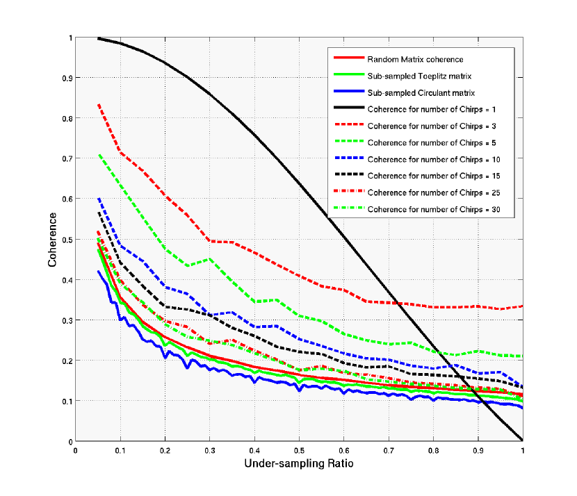
Figure 1: Mutual Coherence of structured sensing matrices as a function of under sampling ratio. Random Gaussian matrix coherence is provided as a baseline. 

We generate 100 realizations of matrices $\mathbf{G},\mathbf{A}$ and $\mathbf{T}$, in order to observe the effect of under-sampling on mutual coherence. It can be seen empirically from figure 1 that the mutual coherence of the sensing matrix $\mathbf{A}$ representing our system converges in mean to the mutual coherence of a sensing matrix $\mathbf{G}$ as the number of chirps increase. We observe that even for small values of $\nu\stackrel{{\scriptstyle\Delta}}{{=}}\frac{N_{c}}{N}=0.03$, the mean of the mutual coherence of our measurement matrix $\mathbf{A}$ is quite close to the mean of the mutual coherence of matrix $\mathbf{G}$. In addition, we also evaluate the coherence of Toeplitz matrix $\mathbf{T}$, which is representative of active-imaging schemes using stochastic waveform that are modeled as linear time invariant systems.

(a) $\mathbf{A}$ with $N_{c}=5$ Chirps

(b) $\mathbf{A}$ with $N_{c}=25$ Chirps

(c) Gaussian sensing matrix $\mathbf{G}$.

(d) Toeplitz sensing matrix $\mathbf{T}$.

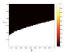
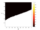
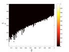
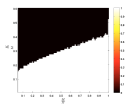
Figure 2: Phase transition curve for the multi-frequency measurement scheme as number of chirps $N_{c}$ increases and other related sensing schemes. Image intensity is either $1$ if reconstruction error is below $1\%$ and $0$ otherwise. We compare the performance of our multi-frequency scheme with other random structured and unstructured matrices as the sparsity level and fractional bandwidth is varied at Signal to Noise ratio of 25 dB.

Next, we consider the recovery performance of our measurement system used in conjunction with Basis pursuit de-noise using SPGL1 solver developed by Van den Berg and Friedlander in [38, 39] to estimate the unknown target locations and their amplitudes in the area of interest. For each realization of the measurement matrix we generate multiple samples of target range profile with specified sparsity level and scattering coefficient is sampled at specified locations are sampled from a complex Gaussian distribution. The overall target range profile is normalized to get a fixed SNR. We consider a function of mean square error as a performance measure, specifically a thresholding function for a fixed SNR of 25dB. We consider a threshold of $1\%$ on the mean squared error and vary both the number of targets in the scene, and the bandwidth of the chirp waveform, which in turn influence the sampling rate at receiver. Again it is clear from figure 2 that the performance becomes similar to that of the random Gaussian sensing matrix $\mathbf{G}$ as the number of chirps increase. We also observe that the recovery performance of Toeplitz matrix $\mathbf{T}$ is similar to our system at lower values of fractional bandwidth $\frac{\beta}{B}\leq 0.7$ but performs better when $\frac{\beta}{B}\geq 0.7$.

(a) $\mathbf{A}$ with $N_{c}=5$ Chirps

(b) $\mathbf{A}$ with $N_{c}=25$ Chirps

(c) Gaussian sensing matrix $\mathbf{G}$

(d) Teoplitz sensing matrix $\mathbf{T}$

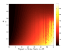
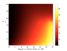
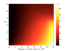
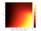
Figure 3: The intensity values of the images represent the reconstruction error in the log scale. Each image from left to right, represents the recovery error for our measurement scheme as number of chirps $N_{c}$ is increased and other measurement schemes as a function of SNR and sparsity level at a fixed fractional bandwidth $\frac{\beta}{B}=0.4$.

Next, we see the influence of noise on sparse target recovery using Basis pursuit de-noise employing our measurement scheme. We fix fractional bandwidth $\frac{\beta}{B}=0.4$ and vary the noise variance as well as the number of targets in the scene. In Figure 3 the intensity of the image represents the mean square error in dB scale. Figure 3 shows that as the number of chirps increase, the performance achieved by our scheme in terms of the mean square error approaches the mean square error achieved by the random Gaussian matrix $\mathbf{G}$. The reconstruction error for Toeplitz matrix $\mathbf{T}$ is marginally better at lower values of $SNR\approx 10dB$ compared to our measurement scheme.

V Proofs

Proof:

The result can be obtained by direct application of lemma 6, using the value of $L=\sqrt{\frac{N}{MN_{c}}}$ and $\nu(\mathbf{A})=\frac{N}{M}$ obtained from lemma 8 and lemma 9, respectively. The upper bound on the tail probability is given as

$$P\left({\left\lVert{\mathbf{A}}\right\rVert_{op}\geq t}\right)\leq\left({N+M}\right)\exp\left({\frac{-t^{2}/2}{\sqrt{\frac{N}{MN_{c}}}\frac{t}{3}+\frac{N}{M}}}\right).$$

By plugging in $t=2\sqrt{\frac{N\log\left({N+M}\right)}{M}}$, we get the result in (1). For the tail probability to decay, we require that $\alpha_{2}>1$. This gives us the condition that $1/3\sqrt{\frac{\log\left({N+M}\right)}{N_{c}}}<0.5$, which implies $N_{c}\geq\frac{4}{9}\log\left({N+M}\right)$. Similarly, using the estimates $L$, and $\nu(\mathbf{A})$ we can bound the expected value of the operator norm of $\mathbf{A}$ as given in lemma 6. ∎

Proof:

The norm of a column m of the sensing matrix $\mathbf{A}$ can be written as follows

$$\left\lVert{\mathbf{A}(m)}\right\rVert_{2}^{2} =\mathbf{c}^{*}\mathbf{B}\mathbf{c},$$

where $\mathbf{B}=\mathbf{G}_{m}^{*}\mathbf{F}^{*}\mathbf{E}_{m}^{*}\mathbf{E}_{m}\mathbf{F}\mathbf{G}_{m}$, and $\mathbf{c}\in\mathbb{R}^{N}$ is a sequence of random variables that selects and scales a subset of the chirp waveforms. It can be verified that the diagonal elements of matrix B are as follows

$$B_{i,i}=\frac{1}{N_{c}},i=1,\cdots,N.$$

Since the random variables $c_{i}$ are independent and $\textbf{E}\left({c_{i}}\right)=0$, the off-diagonal terms vanish and we get

$$\textbf{E}\left({\left\lVert{\mathbf{A}(m)}\right\rVert_{2}^{2}}\right) =\sum_{i=1}^{N}\textbf{E}\left({\left\lvert{c_{i}}\right\rvert^{2}}\right)B_{i,i},$$

$$=\frac{1}{N}\sum_{i=1}^{N}1,$$

$$\textbf{E}\left({\left\lVert{\mathbf{A}(m)}\right\rVert_{2}^{2}}\right) =1.$$

Using results from lemma 10 and lemma 12 along with the result on sub-Gaussian norm from lemma 11, we have

$$P\left({\left\lvert{\left\lVert{\mathbf{A}(m)}\right\rVert_{2}^{2}-1}\right\rvert>t}\right)\leq$$

$$4\exp\left({-\frac{d}{\frac{N_{c}}{N}^{\left({\frac{2}{q^{*}}}\right)}\frac{1}{N_{c}q^{*}}\lceil\frac{N}{M}\rceil}\min\left({\frac{t^{2}}{\frac{N_{c}}{N}^{\left({\frac{2}{q^{*}}}\right)}\frac{M}{N_{c}q^{*}}\lceil\frac{N}{M}\rceil},t}\right)}\right),$$ (21)

$$P\left({\left\lVert{\mathbf{A}(m)}\right\rVert_{2}^{2}<1-t}\right)\leq$$

$$4\exp\left({-\frac{d}{\frac{N_{c}}{N}^{\left({\frac{2}{q^{*}}}\right)}\frac{1}{N_{c}q^{*}}\lceil\frac{N}{M}\rceil}\min\left({\frac{t^{2}}{\frac{N_{c}}{N}^{\left({\frac{2}{q^{*}}}\right)}\frac{M}{N_{c}q^{*}}\lceil\frac{N}{M}\rceil},t}\right)}\right)$$

The concentration inequality for the minimum value of norm of any column can be written as for any $t\in[0,1]$,

$$P\left({\min_{m}\left\lVert{\mathbf{A}(m)}\right\rVert_{2}^{2}\geq 1-t}\right)\geq 1-NP\left({\left\lVert{\mathbf{A}(m)}\right\rVert_{2}^{2}\leq 1-t}\right),$$

$$P\left({\min_{m}\left\lVert{\mathbf{A}(m)}\right\rVert_{2}^{2}\leq 1-t}\right)\leq NP\left({\left\lVert{\mathbf{A}(m)}\right\rVert_{2}^{2}\leq 1-t}\right).$$

Let $t=\epsilon$ for any $\epsilon\leq\frac{\left({\frac{N_{c}}{N}}\right)^{\frac{2}{q^{*}}-1}}{q^{*}}\in(0,1]$. Using the approximation $\left\lceil\frac{N}{M}\right\rceil\approx\frac{N}{M}$, we get the required result. ∎

Proof:

We can express the inner-product between any two columns $m_{1}$ and $m_{2}$ of sensing matrix as

$$\langle{\mathbf{A}(m_{1})},{\mathbf{A}(m_{2})}\rangle=\mathbf{c}^{T}\bar{\mathbf{B}}\mathbf{c},$$

where $\bar{\mathbf{B}}=\mathbf{G}_{m_{1}}^{*}\mathbf{F}^{*}\mathbf{E}_{m_{1}}^{*}\mathbf{E}_{m_{2}}\mathbf{F}\mathbf{G}_{m_{2}}$. The diagonal terms of the matrix $\bar{\mathbf{B}}$ is given as

$$\bar{B}_{i,i}=D_{M}\left({\frac{m_{1}-m_{2}}{N}}\right)\frac{1}{N_{c}}\exp\left({\frac{2\pi j(m_{1}-m_{2})(i-1)}{N}}\right),$$

$$D_{M}\left({\frac{m_{1}-m_{2}}{N}}\right)=\frac{1}{M}\sum_{t=0}^{M-1}\exp\left({2\pi j\left({\frac{m_{1}-m_{2}}{N}}\right)t}\right)$$

where $i=1,\cdots,N$. By using the fact that $c_{i}$ are zero mean independent random variables, we obtain the following expression for $\textbf{E}\left({\mathbf{c}^{T}\bar{\mathbf{B}}\mathbf{c}}\right)$

$$\textbf{E}\left({\mathbf{c}^{T}\bar{\mathbf{B}}\mathbf{c}}\right)=\sum_{i}\textbf{E}\left({c_{i}^{2}}\right)\bar{B}_{i,i}$$

$$=D_{M}\left({\frac{m_{1}-m_{2}}{N}}\right)\sum_{i=1}^{N}\exp\left({\frac{2\pi j(m_{1}-m_{2})(i-1)}{N}}\right)$$

$$=0.$$

Using the results from lemma 10 and lemma 12 along with the sub-Gaussian norm result from lemma 11, and making the approximation $\left\lceil\frac{N}{M}\right\rceil\approx\frac{N}{M}$, we see that there $\exists\ \alpha_{3}>0$ such that

$$P\left({\left\lvert{\langle{\mathbf{A}(m_{1})},{\mathbf{A}(m_{2})}\rangle}\right\rvert>\alpha_{3}\sqrt{\frac{\log N}{M}}}\right)\leq$$

$$4\exp\left({\frac{-q^{*}d\alpha_{3}\log N}{\frac{N_{c}}{N}^{\left({\frac{2}{q^{*}}-1}\right)}}h(N)}\right),$$

where $h(N)=\min\left({\frac{q^{*}\alpha_{3}}{\frac{N_{c}}{N}^{\left({\frac{2}{q^{*}}-1}\right)}},\sqrt{\frac{M}{\log N}}}\right)$. Using the fact that $M\geq(\log N)^{3}$ and $\left\lceil\frac{N}{M}\right\rceil\approx\frac{N}{M}$, we get

$$P\left({\left\lvert{\langle{\mathbf{A}(m_{1})},{\mathbf{A}(m_{2})}\rangle}\right\rvert>\alpha_{3}\sqrt{\frac{\log N}{M}}}\right)$$

$$\leq\begin{cases}\frac{4}{N^{u_{1}}}&\mbox{ if }\log N>\frac{q^{*}}{(\frac{N_{c}}{N})^{(2/q^{*}-1)}}\alpha_{3}\\ \frac{4}{N^{u_{2}}}&\mbox{otherwise, }\end{cases}$$ (22)

where

$$u_{1}=d\left({\frac{q^{*}\alpha_{3}}{\frac{N_{c}}{N}^{\left({\frac{2}{q^{*}}-1}\right)}}}\right)^{2},$$

$$u_{2}=\frac{q^{*}\alpha_{3}}{\frac{N_{c}}{N}^{\left({\frac{2}{q^{*}}-1}\right)}}d\log N.$$

The concentration inequality for the coherence of matrix $\mathbf{A}$ can be obtained by using the following inequality

$$\mu(\mathbf{A}) =\max_{m_{1},m_{2}}\frac{\left\lvert{\langle{\mathbf{A}(m_{1})},{\mathbf{A}(m_{2})}\rangle}\right\rvert}{\left\lVert{\mathbf{A}(m_{1})}\right\rVert\left\lVert{\mathbf{A}(m_{2})}\right\rVert}$$

$$\leq\max_{m_{1},m_{2}}\left\lvert{\langle{\mathbf{A}(m_{1})},{\mathbf{A}(m_{2})}\rangle}\right\rvert\max_{m}\frac{1}{\left\lVert{\mathbf{A}(m)}\right\rVert^{2}}$$

$$P\left({\mu\left({\mathbf{A}}\right)\geq\frac{\alpha_{3}}{1-\epsilon}\sqrt{\frac{\log\left({N}\right)}{M}}}\right)$$

$$\leq P\left({\max_{m_{1},m_{2}}\left\lvert{\langle{\mathbf{A}(m_{1})},{\mathbf{A}(m_{2})}\rangle}\right\rvert\geq\alpha_{3}\sqrt{\frac{\log\left({N}\right)}{M}}}\right)$$

$$+P\left({\min_{m}\left\lVert{\mathbf{A}(m)}\right\rVert^{2}_{2}\leq 1-\epsilon}\right)$$

$$\leq\frac{N^{2}}{2}P\left({\left\lvert{\langle{\mathbf{A}(m_{1})},{\mathbf{A}(m_{2})}\rangle}\right\rvert\geq\alpha_{3}\sqrt{\frac{\log\left({N}\right)}{M}}}\right)$$

$$+P\left({\min_{m}\left\lVert{\mathbf{A}(m)}\right\rVert^{2}_{2}\leq 1-\epsilon}\right)$$

Using (2) and (V) in the above expression, we get the result in (3). ∎

Proof:

Using $M\geq\log(N)^{3}$ and $\log N>\frac{q^{*}}{(\frac{N_{c}}{N})^{(2/q^{*}-1)}}\alpha_{3}$ in (3), the coherence condition given in [26] is satisfied with high probability as shown below

$$\mu\left({\mathbf{A}}\right) =\mathcal{O}\left({\frac{1}{\log N}}\right)$$

w.p. $$p_{1}\geq 1-\frac{2}{N^{u_{1}-2}}+4N\exp\left({-dM\bar{\epsilon}^{2}}\right),$$ (23)

where $\alpha_{3}>0$ is a constant independent of N and M, $\epsilon>0,>1,\epsilon_{1}\in(0,1)$,

$$u_{1}=d\left({\frac{q^{*}\alpha_{3}}{\frac{N_{c}}{N}^{\left({\frac{2}{q^{*}}-1}\right)}}}\right)^{2},$$

and $q^{*}=\max\left({1,2\log\left({\frac{N}{N_{c}}}\right)}\right)$. This establishes the condition in (18). We also note that the exponent in the probability tail bound in (18) depends on $\frac{N_{c}}{N}$ as the function $\frac{N_{c}}{N}^{\left({\frac{2}{q^{*}}-1}\right)}$ is an increasing in $N_{c}\in[0,1/exp(1)]$ but decreases in $N_{c}\in[1/exp(1),1]$. In addition to this, we also believe that $\alpha_{3}$ decreases as $N_{c}$ increases linearly with $N$, which is also verified numerically in section IV. This leads to part of the condition in (19) given as $\frac{N_{c}}{N}\geq\nu\ll 1$.

The measurement matrix in our analysis does not have unit norm columns and in order to apply lemma 5, we normalize the columns. We follow the approach similar to [13]. Let $\mathbf{D}\in\mathbb{R}^{N\times N}$ diagonal matrix with diagonal entries corresponding to the norm of the column of $\mathbf{A}$ given by

$$D_{i,i}=\left\lVert{\mathbf{A}(i)}\right\rVert_{2}.$$

The measurement model can be modified as

$$\mathbf{y}=\hat{\mathbf{A}}\mathbf{z}+\mathbf{w},$$

where $\hat{\mathbf{A}}=\mathbf{A}\mathbf{D}^{-1}$ and $\mathbf{z}=\mathbf{D}\mathbf{x}$. Next, we obtain the probability tail bound for the operator norm of the measurement matrix $\hat{\mathbf{A}}$ with $\ell_{2}$ normalized columns. Using lemma 7, we have $\forall\epsilon>0,\epsilon\in(0,1)$, independent of N and M,

$$P\left({\left\lVert{\hat{\mathbf{A}}}\right\rVert_{op}\geq\frac{2}{\sqrt{1-\epsilon}}\sqrt{\frac{N\log\left({N+M}\right)}{M}}}\right)$$

$$\leq P\left({\left\lVert{\mathbf{A}}\right\rVert_{op}\geq 2\sqrt{\frac{N\log\left({N+M}\right)}{M}}}\right)$$

$$+P\left({\min_{m}D_{m,m}\leq\sqrt{1-\epsilon}}\right)$$

$$\leq\left({\frac{1}{N+M}}\right)^{\alpha_{1}-1}+4N\exp\left({-dM\bar{\epsilon}^{2}}\right),$$

where

$$\alpha_{1}=\frac{2}{1+\frac{2}{3}\sqrt{\frac{\log\left({N+M}\right)}{N_{c}}}},$$

$$N_{c}\geq\frac{4}{9}\log(N+M),$$

$$\bar{\epsilon}=\left({\epsilon\frac{q^{*}}{\left({\frac{N_{c}}{N}}\right)^{\frac{2}{q^{*}}-1}}}\right).$$

Therefore,

$$\left\lVert{\hat{\mathbf{A}}}\right\rVert_{op} \leq\frac{2}{\sqrt{1-\epsilon}}\sqrt{\frac{N\log\left({N+M}\right)}{M}}$$ (24)

w.p. $$p_{2}\geq 1-\left({\frac{1}{N+M}}\right)^{\alpha_{1}-1}+4N\exp\left({-dM\bar{\epsilon}^{2}}\right).$$

This gives us the condition in (19). Using (24) in (32) we obtain the condition in (17).

Next, we establish that the measurement matrix does not reduce the absolute value of non-zero entries of the sparse vector x below the noise level.

$$P\left({\min_{i}D_{i,i}\left\lvert{x_{i}}\right\rvert\leq 8\sigma\sqrt{2\log N}}\right)\leq NP\left({D_{i,i}\leq\sqrt{1-\epsilon}}\right)$$

$$\leq 4N\exp\left({-dM\bar{\epsilon}^{2}}\right).$$

Therefore, we have

$$\min_{i}\left\lvert{z_{i}}\right\rvert\geq 8\sigma\sqrt{2\log N}$$ (25)

w.p. $$p_{3}\geq 1-4N\exp\left({-dM\bar{\epsilon}^{2}}\right).$$

We define the following events associated with a realization of measurement matrix $\mathbf{A}$

$$\Xi_{1}:\mu\left({\mathbf{A}}\right)=\mathcal{O}\left({\frac{1}{\log N}}\right)$$

$$\Xi_{2}:\left\lVert{\hat{\mathbf{A}}}\right\rVert^{2}_{op}\leq\frac{c_{0}N}{K_{\max}\log N}$$

$$\Xi_{3}:\min_{i}\left\lvert{z_{i}}\right\rvert\geq 8\sigma\sqrt{2\log N}.$$

$$\Xi_{4}:\mbox{successful support recovery for a fixed sensing matrix}.$$

Let $\Xi$ be the event that the sampled measurement matrix satisfies the conditions required for successful recovery and recovers a K-sparse vector $\mathbf{x}$ selected from the target model. This implies

$$P\left({\Xi}\right) \geq P\left({\Xi_{4}\mid\Xi_{1}\cap\Xi_{2}\cap\Xi_{3}}\right)\times$$

$$(1-P\left({\Xi^{c}_{1}}\right)-P\left({\Xi^{c}_{2}}\right)-P\left({\Xi^{c}_{3}}\right)).$$ (26)

Using result from Lemma 5 for $P\left({\Xi_{4}\mid\Xi_{1}\cap\Xi_{2}\cap\Xi_{3}}\right)$,(24), (25) and (V) in (V), we get the desired recovery guarantee. ∎

Proof:

Using $\delta_{K}\leq\delta+\epsilon$ in (I), it can be deduced that the eigen values of $\mathbf{A}^{*}_{\Gamma}\mathbf{A}_{\Gamma},\forall\Gamma$ are $\in\left[{1-\delta-\epsilon,1+\delta+\epsilon}\right]$ such that $card\left({\Gamma}\right)\leq K$. This can be translated into a condition on the elements of the Gramian matrix $\mathbf{A}^{*}\mathbf{A}$ using lemma 4 given as the following events $\Xi_{5}:\bigcap_{\stackrel{{\scriptstyle m_{1},m_{2}}}{{m_{1}\neq m_{2}}}}\left\{{\left\lvert{\langle{\mathbf{A(m_{1})}},{\mathbf{A(m_{2})}}\rangle}\right\rvert\leq\frac{\delta}{K}}\right\}$ $\Xi_{6}:\bigcap_{m=1}^{M}\left\{{\left\lvert{\left\lVert{\mathbf{A}(m)}\right\rVert_{2}^{2}-1}\right\rvert\leq\epsilon}\right\}.$

Let $\Xi$ be the event denoting that the RIP condition of order $K$ is satisfied. Then we have

$$P(\Xi^{c}) \leq 1-\frac{N^{2}}{2}P\left({\left\lvert{\langle{\mathbf{A(m_{1})}},{\mathbf{A(m_{2})}}\rangle}\right\rvert\geq\frac{\delta}{K}}\right)$$

$$\qquad-NP\left({\left\lvert{\left\lVert{\mathbf{A}(m)}\right\rVert_{2}^{2}-1}\right\rvert\geq\epsilon}\right)$$ (27)

Using the result from (V) and using the fact that we can choose $N_{c}$ such that $\epsilon\leq\frac{q^{*}}{\frac{N_{c}}{N}^{\left({\frac{2}{q^{*}}-1}\right)}}$, we get

$$P\left({\left\lvert{\left\lVert{\mathbf{A}(m)}\right\rVert_{2}^{2}-1}\right\rvert\geq\epsilon}\right)\leq 4\exp\left({-d\left({\epsilon\frac{q^{*}}{\frac{N_{c}}{N}^{\left({\frac{2}{q^{*}}-1}\right)}}}\right)^{2}M}\right)$$ (28)

Similarly, using results from lemma 3 we can obtain

$$P\left({\left\lvert{\langle{\mathbf{A(m_{1})}},{\mathbf{A(m_{2})}}\rangle}\right\rvert\geq\frac{\delta}{K}}\right)\leq$$

$$\qquad 4\exp\left({-dM\frac{\delta^{2}}{K^{2}}\left({\frac{q^{*}}{\frac{N_{c}}{N}^{\left({\frac{2}{q^{*}}-1}\right)}}}\right)^{2}}\right).$$ (29)

Using (28), (V) and the condition that $M\geq a\delta^{-2}K^{2}\log N$ in (V) we get the desired results. ∎

VI Conclusion

In this work we have shown that structured compressed sensing matrices with random components can be realized in radar (delay estimation) setting using an LFM waveform modulated by a random sparse multi-tone signal in transmit and a simple traditional analog receiver structure. We provide recovery guarantees for the proposed compressive sensor comparable to random Toeplitz/Circular matrices with much larger number of random elements. The proposed scheme is well matched to practical implementation utilizing small number of random parameters and uniform sampling ADCs on receive.

A potential direction for future research is to investigate the effectiveness of multi-chirp waveforms in the multiple output multiple input (MIMO) setting with multiple transmit and receive antenna elements for estimating support of targets in angle and range domain [13]. We note that in this setting each transmitter can use a single chirp with a random frequency offset and superposition is achieved at each receiver as the waveforms reflected from the scene is naturally summed at each receiver.

[Some Useful Lemmas]

Lemma 4

Given a complex matrix $M\in\mathbb{C}^{n\times n}$ with $C_{i}=M_{i,i}$, and $R_{i}=\sum_{j\neq i}\left\lvert{M_{i,j}}\right\rvert$ then we have

$$\lambda_{i}\in\cup_{i=1}^{n}D(C_{i},R_{i}),\forall i=1,\cdots,n,$$ (30)

where $D(c,r)$ is a disc with center c and radius r, and $\lambda_{i}$ are the eigen-values of M.

We restate the theorem given in [13], which was extended to the complex setting in [26], that give the conditions on the measurement matrix for successful recovery when using $\ell_{1}$ penalized optimization methods.

Lemma 5

For a measurement model $\mathbf{y}=\mathbf{A}\mathbf{x}+\mathbf{w}$, where $\mathbf{A}\in\mathbb{C}^{M\times N}$ has unit $\ell_{2}$ norm columns, $\mathbf{x}$ is drawn from a K-sparse model in complex domain and $w_{i}\sim\mathcal{CN}(0,\sigma^{2})$, if the following conditions are satisfied

$$\mu(\mathbf{A})\leq\frac{\alpha_{0}}{\log N},$$ (31)

where $\alpha_{0}>0$ is a constant independent of the dimensions of the problem; also, if

$$K\leq K_{\max}\left({\mathbf{A}}\right)=\frac{\alpha_{1}N}{\left\lVert{\mathbf{A}}\right\rVert_{op}^{2}\log\left({N}\right)},$$ (32)

for some $\alpha_{1}>0$, and

$$\min_{k\in I}\left\lvert{x_{k}}\right\rvert>8\sigma\sqrt{2\log\left({N}\right)},$$ (33)

then the solution $\hat{\mathbf{x}}$ of (12) has the same support as the unknown sparse vector $\mathbf{x}$ and relative error is bounded as shown below

$$\emph{supp}(\hat{\mathbf{x}})=\emph{supp}(\mathbf{x})$$ (34)

$$Pr\left({\frac{\left\lVert{\hat{\mathbf{x}}-\mathbf{x}}\right\rVert_{2}}{\left\lVert{\mathbf{x}}\right\rVert_{2}}\leq\frac{\sigma\sqrt{3N}}{\left\lVert{\mathbf{y}}\right\rVert_{2}}}\right)$$

$$\geq 1-2N^{-1}(2\pi\log\left({N}\right)+KN^{-1})-\mathcal{O}\left({N^{-2\log 2}}\right).$$ (35)

Lemma 6 (Matrix Bernstein inequality [40])

Let $\mathbf{A}_{i}$ be a sequence of i.i.d. random matrices. For a random matrix expressed as $\mathbf{A}=\sum_{i}\mathbf{A}_{i}$ we have

$$P\left({\left\lVert{\mathbf{A}}\right\rVert_{op}\geq t}\right)\leq\left({d_{1}+d_{2}}\right)\exp\left({\frac{-t^{2}/2}{\frac{Lt}{3}+\nu\left({\mathbf{A}}\right)}}\right),$$ (36)

$$\left\lVert{\mathbf{A}_{i}}\right\rVert_{op}\leq L,\forall i=1,\cdots,D$$

$$\nu\left({\mathbf{A}}\right)=\max\left({\textbf{E}\left({\mathbf{A}\mathbf{A}^{*}}\right),\textbf{E}\left({\mathbf{A}^{*}\mathbf{A}}\right)}\right),$$

where $\mathbf{A}_{i}\in\mathbb{C}^{d_{1}\times d_{2}}$. The expected value of the operator norm of $\mathbf{A}$ is bounded by

$$\textbf{E}\left({\left\lVert{\mathbf{A}}\right\rVert_{op}}\right)\leq\sqrt{2\nu\left({\mathbf{A}}\right)\log\left({d_{1}+d_{2}}\right)}+\frac{L\log\left({d_{1}+d_{2}}\right)}{3}.$$ (37)

Lemma 7

Given a matrix $\mathbf{A}$, the operator norm of the matrix $\hat{\mathbf{A}}=\mathbf{A}\mathbf{D}^{-1}$ is bounded by the following inequality

$$\frac{\left\lVert{\mathbf{A}}\right\rVert_{op}}{\min_{i}D_{i,i}}\geq\left\lVert{\hat{\mathbf{A}}}\right\rVert_{op}\geq\frac{\left\lVert{\mathbf{A}}\right\rVert_{op}}{\max_{i}D_{i,i}},$$ (38)

where $\mathbf{D}$ is a diagonal matrix with positive diagonal elements.

Proof:

For any vector $\mathbf{v}$ such that $\left\lVert{\mathbf{v}}\right\rVert_{2}=1$, we have

$$\bar{\mathbf{A}}\mathbf{v}=\frac{\mathbf{A}\mathbf{D}^{-1}\mathbf{v}}{\left\lVert{\mathbf{D}^{-1}\mathbf{v}}\right\rVert_{2}}\left\lVert{\mathbf{D}^{-1}\mathbf{v}}\right\rVert_{2}=\mathbf{A}\mathbf{u(v)}\left\lVert{\mathbf{D}^{-1}\mathbf{v}}\right\rVert_{2}$$

$$\implies \left\lVert{\bar{\mathbf{A}}\mathbf{v}}\right\rVert_{2}=\left\lVert{\mathbf{A}\mathbf{u(v)}}\right\rVert_{2}\left\lVert{\mathbf{D}^{-1}\mathbf{v}}\right\rVert_{2},$$

where $\mathbf{u(v)}=\frac{\mathbf{D}^{-1}\mathbf{v}}{\left\lVert{\mathbf{D}^{-1}\mathbf{v}}\right\rVert_{2}}$. Since $\left\lVert{\mathbf{v}}\right\rVert_{2}=1$, we bound the Euclidean norm of $\mathbf{D}^{-1}v$ as follows

$$\frac{1}{\min_{i}D_{i,i}}\geq\left\lVert{\mathbf{D}^{-1}\mathbf{v}}\right\rVert_{2}\geq\frac{1}{\max_{i}D_{i,i}}.$$

Using this we get,

$$\frac{\left\lVert{\mathbf{A}\mathbf{u(v)}}\right\rVert_{2}}{\min_{i}D_{i,i}}\geq\left\lVert{\bar{\mathbf{A}}\mathbf{v}}\right\rVert_{2}\geq\frac{\left\lVert{\mathbf{A}\mathbf{u(v)}}\right\rVert_{2}}{\max_{i}D_{i,i}}.$$

By taking supremum over $\mathbf{v}$ in the space of unit norm vectors we obtain the desired result. ∎

Lemma 8

For the matrix $c_{i}\mathbf{H}_{i}\bar{\mathbf{A}}\mathbf{D}_{i}\in\mathbb{C}^{M\times N}$ in (II-A), we have

$$\left\lVert{c_{i}\mathbf{H}_{i}\bar{\mathbf{A}}\mathbf{D}_{i}}\right\rVert_{op}\leq\sqrt{\frac{N}{MN_{c}}},$$ (39)

$\forall i=1,\cdots,N$

Proof:

By sub-multiplicativity property of the operator norm we have,

$$\left\lVert{c_{i}\mathbf{H}_{i}\bar{\mathbf{A}}\mathbf{D}_{i}}\right\rVert_{op}\leq\left\lvert{c_{i}}\right\rvert\left\lVert{\mathbf{H}_{i}}\right\rVert_{op}\left\lVert{\bar{\mathbf{A}}}\right\rVert_{op}\left\lVert{\mathbf{D}_{i}}\right\rVert_{op}.$$

Since $\mathbf{H}_{i}$ and $\mathbf{D}_{i}$ are diagonal matrices with complex exponential entries, it can be shown that $\left\lVert{\mathbf{H}_{i}}\right\rVert_{op}=\left\lVert{\mathbf{D}_{i}}\right\rVert_{op}=1$. Also, we assume that $c_{i}$ are sub-Gaussian random variables with $\left\lvert{c_{i}}\right\rvert\leq 1$. In order to find the operator norm of $\bar{\mathbf{A}}$, we define $\mathbf{G}=\bar{\mathbf{A}}\bar{\mathbf{A}}^{*}\in\mathbf{C}^{M\times M}$ since it is full rank and $\left\lVert{\bar{\mathbf{A}}}\right\rVert^{2}_{op}=\left\lVert{\mathbf{G}}\right\rVert_{op}$. The entries of matrix $\mathbf{G}$ are as follows

$$G(k,k)=\frac{N}{MN_{c}}$$

$$G(k,l)=\frac{N}{MN_{c}}\frac{1}{N}\sum_{m=0}^{N-1}\exp\left({2\pi j\frac{l-k}{N}m}\right)$$

$$=\frac{N}{MN_{c}}D_{N}\left({\frac{l-k}{N}}\right)=0,$$

$\forall k,l=0,\cdots,M-1$, such that $k\neq l$, and $D_{N}\left({\frac{l-k}{N}}\right)=\frac{1}{N}\sum_{m=0}^{N-1}\exp\left({2\pi j\frac{l-k}{N}m}\right)$ is the discrete Dirichlet Kernel. The second term is zero because the discrete Dirichlet kernel is being evaluated at it’s zeros, which are the Fourier frequency bins $(\frac{n}{N}),n\in\mathbb{Z}$. Therefore,

$$\mathbf{G}=\frac{N}{MN_{c}}\mathbf{I}.$$

This implies that the $\left\lVert{\mathbf{G}}\right\rVert_{op}=\frac{N}{MN_{c}}$ and leads to the result in (39). ∎

Lemma 9

For the matrices $\mathbf{P}_{i}=c_{i}\mathbf{H}_{i}\bar{\mathbf{A}}\mathbf{D}_{i}\in\mathbb{C}^{M\times N}$ given by (II-A), we have

$$\left\lVert{\sum_{i=1}^{N}\textbf{E}\left({\mathbf{P}_{i}^{*}\mathbf{P}_{i}}\right)}\right\rVert \leq\frac{N}{M},$$ (40)

$$\left\lVert{\sum_{i=1}^{N}\textbf{E}\left({\mathbf{P}_{i}\mathbf{P}_{i}^{*}}\right)}\right\rVert =\frac{N}{M}.$$ (41)

Proof:

First, we compute the norm of $\mathbf{P}_{i}\mathbf{P}_{i}^{*}$ as it is a full-rank matrix using $\mathbf{D}_{i}\mathbf{D}_{i}^{*}=\mathbf{I}$, $\mathbf{H}_{i}\mathbf{H}_{i}^{*}=\mathbf{I}$ and $\bar{\mathbf{A}}\bar{\mathbf{A}}^{*}=\frac{N}{MN_{c}}\mathbf{I}$ we have

$$\mathbf{P}_{i}\mathbf{P}_{i}^{*} =c_{i}c_{i}^{*}\mathbf{H}_{i}\bar{\mathbf{A}}\mathbf{D}_{i}\mathbf{D}_{i}^{*}\bar{\mathbf{A}}^{*}\mathbf{H}_{i}^{*}$$

$$=c_{i}c_{i}^{*}\frac{N}{MN_{c}}\mathbf{I}.$$

Using the probabilistic model for $c_{i}$ given in (2), we get

$$\textbf{E}\left({c_{i}c_{i}^{*}}\right)=\frac{N_{c}}{N}.$$

We have

$$\sum_{i=1}^{N}\textbf{E}\left({\mathbf{P}_{i}\mathbf{P}_{i}^{*}}\right) =\frac{N}{M}\mathbf{I}.$$

Applying the operator norm yields the result in (41). Similarly, using the sub-additivity of the operator norm and $\left\lVert{\mathbf{H}_{i}\bar{\mathbf{A}}\mathbf{D}_{i}\mathbf{D}_{i}^{*}\bar{\mathbf{A}}^{*}\mathbf{H}_{i}^{*}}\right\rVert_{op}=\left\lVert{\mathbf{D}^{*}_{i}\bar{\mathbf{A}}^{*}\mathbf{H}^{*}_{i}\mathbf{H}_{i}\bar{\mathbf{A}}\mathbf{D}_{i}}\right\rVert_{op}$ we get

$$\left\lVert{\sum_{i=1}^{N}\textbf{E}\left({\mathbf{P}_{i}^{*}\mathbf{P}_{i}}\right)}\right\rVert_{op} =\left\lVert{\sum_{i=1}^{N}\textbf{E}\left({c_{i}^{*}c_{i}}\right)\mathbf{D}^{*}_{i}\bar{\mathbf{A}}^{*}\mathbf{H}^{*}_{i}\mathbf{H}_{i}\bar{\mathbf{A}}D_{i}}\right\rVert_{op}$$

$$\leq\sum_{i=1}^{N}\left\lvert{\textbf{E}\left({c_{i}c_{i}^{*}}\right)}\right\rvert\left\lVert{\mathbf{H}_{i}\bar{\mathbf{A}}\mathbf{D}_{i}\mathbf{D}_{i}^{*}\bar{\mathbf{A}}^{*}\mathbf{H}_{i}^{*}}\right\rVert_{op}$$

$$=\frac{N}{M}.$$

∎

Lemma 10

Let $\mathbf{B}=\mathbf{G}_{m}^{*}\mathbf{F}^{*}\mathbf{E}_{m}^{*}\mathbf{E}_{m}\mathbf{F}\mathbf{G}_{m}$, and $\bar{\mathbf{B}}=\mathbf{G}_{m_{1}}^{*}\mathbf{F}^{*}\mathbf{E}_{m_{1}}^{*}\mathbf{E}_{m_{2}}\mathbf{F}\mathbf{G}_{m_{2}}$ then we have

$$\left\lVert{\mathbf{B}}\right\rVert_{op}\leq\left\lceil\frac{N}{M}\right\rceil\frac{1}{N_{c}}, \left\lVert{\mathbf{B}}\right\rVert_{F}\leq\left\lceil\frac{N}{M}\right\rceil\frac{\sqrt{M}}{N_{c}},$$ (42)

$$\left\lVert{\bar{\mathbf{B}}}\right\rVert_{op}\leq\left\lceil\frac{N}{M}\right\rceil\frac{1}{N_{c}}, \left\lVert{\bar{\mathbf{B}}}\right\rVert_{F}\leq\left\lceil\frac{N}{M}\right\rceil\frac{\sqrt{M}}{N_{c}},$$ (43)

where $\lceil x\rceil=z\in\mathbb{Z}$ such that $z\geq x,\ \forall x\in\mathbb{R}$.

Proof:

We note that $Rank(\mathbf{B})=Rank(\bar{\mathbf{B}})=M$, and we can obtain a bound on the Frobenius norm of the matrices as shown below

$$\left\lVert{\mathbf{B}}\right\rVert_{F} \leq\sqrt{M}\left\lVert{\mathbf{B}}\right\rVert_{op},$$

$$\left\lVert{\bar{\mathbf{B}}}\right\rVert_{F} \leq\sqrt{M}\left\lVert{\bar{\mathbf{B}}}\right\rVert_{op}.$$

In order to find the bound on the operator norm we see that

$$\left\lVert{\mathbf{B}}\right\rVert_{op} \leq\left\lVert{\mathbf{G}_{m}}\right\rVert_{op}^{2}\left\lVert{\mathbf{E}_{m}}\right\rVert_{op}^{2}\left\lVert{\mathbf{F}}\right\rVert^{2},$$

$$\left\lVert{\bar{\mathbf{B}}}\right\rVert_{op} \leq\left\lVert{\mathbf{G}_{m_{1}}}\right\rVert_{op}\left\lVert{\mathbf{G}_{m_{2}}}\right\rVert_{op}\left\lVert{\mathbf{E}_{m_{1}}}\right\rVert_{op}\left\lVert{\mathbf{E}_{m_{2}}}\right\rVert_{op}\left\lVert{\mathbf{F}}\right\rVert^{2}.$$

Since $\mathbf{G}_{m}$ and $\mathbf{E}_{m}$ are diagonal matrices with complex exponentials along the principal diagonal, it can be shown that $\left\lVert{\mathbf{G}_{m}}\right\rVert_{op}^{2}=\left\lVert{\mathbf{E}_{m}}\right\rVert_{op}^{2}=1$. In order to estimate the $\left\lVert{\mathbf{F}}\right\rVert_{op}$, we see that

$$\mathbf{F}^{*}\mathbf{F}=\frac{1}{N_{c}}\begin{bmatrix}\mathbf{V}_{1,1}&\cdots&\mathbf{V}_{1,\left\lceil\frac{N}{M}\right\rceil}\\ \mathbf{V}_{2,1}&\cdots&\mathbf{V}_{2,\left\lceil\frac{N}{M}\right\rceil}\\ \vdots&\vdots&\vdots\\ \mathbf{V}_{\left\lceil\frac{N}{M}\right\rceil,1}&\cdots&\mathbf{V}_{2,\left\lceil\frac{N}{M}\right\rceil}\end{bmatrix}$$

Since $p$ is co-prime with $M$, we observe that the N possible frequency tones circularly get mapped onto M possible aliased sinusoids. Therefore, if neither $i,j\neq\left\lceil\frac{N}{M}\right\rceil$,

$$\mathbf{V}_{i,j}=\mathbf{I}.$$

If either $i=\left\lceil\frac{N}{M}\right\rceil$ or $j=\left\lceil\frac{N}{M}\right\rceil$, then $\mathbf{V}_{i,j}\in\mathbb{C}^{M\times M}$ is a partial identity matrix. It can easily be verified that $\left\lVert{\mathbf{F}}\right\rVert_{op}^{2}=\frac{1}{N_{c}}\left\lceil\frac{N}{M}\right\rceil$. Using this result along-with the estimate on the bound for the Frobenius norm, we get the desired results. ∎

Lemma 11

For the sub-Gaussian random variables described in (2) and (4), the Sub-Gaussian norm [41] is as follows

$$\left\lVert{C_{i}}\right\rVert_{\Psi_{2}}=\sup_{q\geq 1}\textbf{E}\left({\left\lvert{C_{i}}\right\rvert^{q}}\right)^{\frac{1}{q}}\frac{1}{\sqrt{q}}$$

$$\left\lVert{C_{i}}\right\rVert_{\Psi_{2}}=\left({\frac{N_{c}}{N}}\right)^{\frac{1}{q^{*}}}\frac{1}{\sqrt{q^{*}}},$$ (44)

$$q^{*}=\max\left({1,2\log\left({\frac{N}{N_{c}}}\right)}\right).$$

Proof:

For the probability models given in (2) and (4), we have

$$\left\lvert{C_{i}}\right\rvert=\begin{cases}0&\mbox{ with probability }1-\frac{N_{c}}{N}\\ 1&\mbox{w.p. }\frac{N_{c}}{N}.\end{cases}$$

$$\textbf{E}\left({\left\lvert{C_{i}}\right\rvert^{q}}\right)^{\frac{1}{q}}=\left({\frac{N_{c}}{N}}\right)^{\frac{1}{q}}.$$

$$\implies \left\lVert{C_{i}}\right\rVert_{\Psi_{2}}=\sup_{q\geq 1}\left({\frac{N_{c}}{N}}\right)^{\frac{1}{q}}\frac{1}{\sqrt{q}}.$$

The solution to this optimization problem can be found by taking the logarithm and solving the unconstrained optimization problem which is given as

$$q^{*}=2\log\left({\frac{N}{N_{c}}}\right).$$

In order to satisfy the constraint, the solution is lower bounded by 1. ∎

Lemma 12

Given a zero mean real random vector $\mathbf{c}$ composed of independent and sub-Gaussian random variables $c_{i},i=1,\cdots,N$ such that $\left\lVert{c_{i}}\right\rVert_{\Psi_{2}}\leq K$, $i=1,\cdots,N$, we have

$$Pr\left({\left\lvert{\mathbf{c}^{T}\mathbf{B}\mathbf{c}-\textbf{E}\left({\mathbf{c}^{T}\mathbf{B}\mathbf{c}}\right)}\right\rvert>t}\right)$$

$$\leq 4\exp\left({-d\min\left({\frac{t^{2}}{K^{4}\left\lVert{\mathbf{B}}\right\rVert_{F}^{2}},\frac{t}{K^{2}\left\lVert{\mathbf{B}}\right\rVert_{op}}}\right)}\right),$$ (45)

where $\mathbf{B}\in\mathbb{C}^{N\times N}$, $\mathbf{c}\in\mathbb{R}^{N}$, for some absolute constant $d>0$ and $\forall t>0$.

Proof:

Let $\mathbf{B}=\mathbf{B}_{R}+i\mathbf{B}_{Im}$, where $\mathbf{B}_{R},\mathbf{B}_{Im}\in\mathbb{R}^{N\times N}$. Therefore, using the Hanson-Wright inequality for real matrices given in [36] and the fact that $\left\lVert{\mathbf{B}_{R}}\right\rVert_{op}\leq\left\lVert{\mathbf{B}}\right\rVert_{op}$, $\left\lVert{\mathbf{B}_{Im}}\right\rVert_{op}\leq\left\lVert{\mathbf{B}}\right\rVert_{op}$, and $\left\lVert{\mathbf{B}_{R}}\right\rVert_{F}\leq\left\lVert{\mathbf{B}}\right\rVert_{F}$, $\left\lVert{\mathbf{B}_{Im}}\right\rVert_{F}\leq\left\lVert{\mathbf{B}}\right\rVert_{F}$ we have

$$Pr \left({\left\lvert{\mathbf{c}^{T}\mathbf{B}\mathbf{c}-\textbf{E}\left({\mathbf{c}^{T}\mathbf{B}\mathbf{c}}\right)}\right\rvert>t}\right)\leq$$

$$Pr\left({\left\lvert{\mathbf{c}^{T}\mathbf{B}_{R}\mathbf{c}-\textbf{E}\left({\mathbf{c}^{T}\mathbf{B}_{R}\mathbf{c}}\right)}\right\rvert>\frac{t}{\sqrt{2}}}\right)+$$

$$Pr\left({\left\lvert{\mathbf{c}^{T}\mathbf{B}_{Im}\mathbf{c}-\textbf{E}\left({\mathbf{c}^{T}\mathbf{B}_{Im}\mathbf{c}}\right)}\right\rvert>\frac{t}{\sqrt{2}}}\right).$$

This gives us the inequality in (12). ∎

References

• [1] M. A. Richards, Fundamentals of Radar Signal Processing.   New York, NY, USA: McGraw-Hill, 2014.
• [2] R. Middleton, “Dechirp-on-receive linearly frequency modulated radar as a matched-filter detector,” IEEE Transactions on Aerospace and Electronic Systems, vol. 48, no. 3, pp. 2716–2718, July 2012.
• [3] D. L. Donoho, “Compressed sensing,” IEEE Transactions on Information Theory, vol. 52, no. 4, pp. 1289–1306, Apr. 2006.
• [4] E. Candes, J. Romberg, and T. Tao, “Robust uncertainty principles: exact signal reconstruction from highly incomplete frequency information,” IEEE Transactions on Information Theory, vol. 52, no. 2, pp. 489–509, Feb. 2006.
• [5] E. Candes and T. Tao, “The dantzig selector: Statistical estimation when p is much larger than n,” The Annals of Statistics, vol. 35, no. 6, pp. 2313–2351, Dec. 2007.
• [6] S. S. Chen, D. L. Donoho, and M. A. Saunders, “Atomic decomposition by basis pursuit,” SIAM Rev., vol. 43, no. 1, pp. 129–159, Jan. 2001.
• [7] R. Tibshirani, “Regression shrinkage and selection via the lasso,” Journal of the Royal Statistical Society: Series B, vol. 73, no. 3, pp. 273–282, 1996.
• [8] J. Tropp and A. Gilbert, “Signal recovery from random measurements via orthogonal matching pursuit,” IEEE Transactions on Information Theory, vol. 53, no. 12, pp. 4655–4666, Dec. 2007.
• [9] D. Needell and J. Tropp, “Cosamp: Iterative signal recovery from incomplete and inaccurate samples,” Applied and Computational Harmonic Analysis, vol. 26, no. 3, pp. 301 – 321, 2009.
• [10] L. Potter, E. Ertin, J. Parker, and M. Cetin, “Sparsity and compressed sensing in radar imaging,” Proceedings of the IEEE, vol. 98, no. 6, pp. 1006–1020, June 2010.
• [11] K. Gedalyahu and Y. Eldar, “Time-delay estimation from low-rate samples: A union of subspaces approach,” IEEE Transactions on Signal Processing,, vol. 58, no. 6, pp. 3017–3031, June 2010.
• [12] M. Herman and T. Strohmer, “High-resolution radar via compressed sensing,” IEEE Transactions on Signal Processing, vol. 57, no. 6, pp. 2275–2284, June 2009.
• [13] T. Strohmer and B. Friedlander, “Analysis of sparse mimo radar,” Applied and Computational Harmonic Analysis, vol. 37, no. 3, pp. 361 – 388, 2014.
• [14] T. Strohmer and H. Wang, “Accurate imaging of moving targets via random sensor arrays and kerdock codes,” Inverse Problems, vol. 29, no. 8, p. 085001, 2013.
• [15] M. HÃŒgel, H. Rauhut, and T. Strohmer, “Remote sensing via 1subscript1\ell_{1}-minimization,” Foundations of Computational Mathematics, vol. 14, no. 1, pp. 115–150, 2014.
• [16] M. Rossi, A. Haimovich, and Y. Eldar, “Spatial compressive sensing in mimo radar with random arrays,” in Information Sciences and Systems (CISS), 2012 46th Annual Conference on, Mar. 2012, pp. 1–6.
• [17] M. Shastry, R. Narayanan, and M. Rangaswamy, “Sparsity-based signal processing for noise radar imaging,” IEEE Transactions on Aerospace and Electronic Systems, vol. 51, no. 1, pp. 314–325, Jan. 2015.
• [18] E. Baransky, G. Itzhak, N. Wagner, I. Shmuel, E. Shoshan, and Y. Eldar, “Sub-nyquist radar prototype: Hardware and algorithm,” IEEE Transactions on Aerospace and Electronic Systems,, vol. 50, no. 2, pp. 809–822, Apr. 2014.
• [19] J. Yoo, C. Turnes, E. Nakamura, C. Le, S. Becker, E. Sovero, M. Wakin, M. Grant, J. Romberg, A. Emami-Neyestanak, and E. Candes, “A compressed sensing parameter extraction platform for radar pulse signal acquisition,” IEEE Journal on Emerging and Selected Topics in Circuits and Systems, vol. 2, no. 3, pp. 626–638, Sep. 2012.
• [20] J. Tropp, J. Laska, M. Duarte, J. Romberg, and R. Baraniuk, “Beyond nyquist: Efficient sampling of sparse bandlimited signals,” IEEE Transactions on Information Theory, vol. 56, no. 1, pp. 520–544, Jan. 2010.
• [21] M. Duarte and R. Baraniuk, “Spectral compressive sensing,” Applied and Computational Harmonic Analysis, vol. 35, no. 1, pp. 111 – 129, 2013.
• [22] A. Gilbert, M. Strauss, and J. Tropp, “A tutorial on fast fourier sampling,” IEEE Signal Processing Magazine, vol. 25, no. 2, pp. 57–66, Mar. 2008.
• [23] E. Ertin, “Frequency diverse waveforms for compressive radar sensing,” in Waveform Diversity and Design Conference (WDD), 2010 International, Aug. 2010, pp. 000 216–000 219.
• [24] E. Ertin, L. Potter, and R. Moses, “Sparse target recovery performance of multi-frequency chirp waveforms,” in 19th European Signal Processing Conference, 2011, Aug 2011, pp. 446–450.
• [25] T. T. Cai and T. Jiang, “Limiting laws of coherence of random matrices with applications to testing covariance structure and construction of compressed sensing matrices,” The Annals of Statistics, vol. 39, no. 3, pp. 1496–1525, June 2011.
• [26] E. Candes and Y. Plan, “Near-ideal model selection by ℓ1 minimization,” The Annals of Statistics, vol. 37, no. 5A, pp. 2145–2177, Oct. 2009.
• [27] K. Davidson and S. Szarek, “Local operator theory, random matrices and banach spaces,” Handbook on the Geometry of Banach spaces, vol. 1, pp. 317–366, 2001.
• [28] W. Bajwa, “Geometry of random toeplitz-block sensing matrices: bounds and implications for sparse signal processing,” Proc. SPIE, vol. 8365, pp. 836 505–836 505–7, 2012.
• [29] E. Candes, “The restricted isometry property and its implications for compressed sensing,” Comptes Rendus Mathematique, vol. 346, no. 9-10, pp. 589–592, May 2008.
• [30] R. Baraniuk, M. Davenport, R. A. DeVore, and M. B. Wakin, “A simple proof of the restricted isometry property for random matrices,” Constructive Approximation, vol. 28, no. 3, pp. 253–263, Dec. 2008.
• [31] J. Haupt, W. Bajwa, G. Raz, and R. Nowak, “Toeplitz compressed sensing matrices with applications to sparse channel estimation,” IEEE Transactions on Information Theory, vol. 56, no. 11, pp. 5862–5875, Nov. 2010.
• [32] J. Romberg, “Compressive sensing by random convolution,” SIAM J. Img. Sci., vol. 2, no. 4, pp. 1098–1128, Nov. 2009.
• [33] H. Rauhut, J. Romberg, and J. A. Tropp, “Restricted isometries for partial random circulant matrices,” Applied and Computational Harmonic Analysis, vol. 32, no. 2, pp. 242 – 254, 2012.
• [34] F. Krahmer, S. Mendelson, and H. Rauhut, “Suprema of chaos processes and the restricted isometry property,” Communications on Pure and Applied Mathematics, vol. 67, no. 11, pp. 1877–1904, 2014.
• [35] S. Foucart and H. Rauhut, A Mathematical Introduction to Compressive Sensing.   Birkhauser Basel, 2013.
• [36] M. Rudelson and R. Vershynin, “Hanson-wright inequality and sub-gaussian concentration,” Electron. Commun. Probab., vol. 18, pp. no. 82, 1–9, 2013.
• [37] J. Tropp, “Norms of random submatrices and sparse approximation,” Comptes Rendus Mathematique, vol. 346, no. 23–24, pp. 1271 – 1274, 2008.
• [38] E. van den Berg and M. P. Friedlander, “SPGL1: A solver for large-scale sparse reconstruction,” June 2007, http://www.cs.ubc.ca/labs/scl/spgl1.
• [39] ——, “Probing the pareto frontier for basis pursuit solutions,” SIAM Journal on Scientific Computing, vol. 31, no. 2, pp. 890–912, 2008.
• [40] J. Tropp, “An Introduction to Matrix Concentration Inequalities,” ArXiv e-prints, Jan. 2015.
• [41] R. Vershynin, Introduction to the non-asymptotic analysis of random matrices -Compressed sensing, 210–268.   Cambridge, USA: Cambridge Univ. Press, 2012.