Infrared multiphoton resummation in quantum electrodynamics

Abstract

Infrared singularities in massless gauge theories are known since the foundation of quantum field theories. The root of this problem can be tracked back to the very definition of these long-range interacting theories such as QED. It can be shown that singularities are caused by the massless degrees of freedom (i.e. the photons in the case of QED). In the Bloch-Nordsieck model the absence of the infrared catastrophe can be shown exactly by the complete summation of the radiative corrections. In this paper we will give the idea of the derivation of the Bloch-Nordsieck propagator, that describes the infrared structure of the electron propagation, at zero and finite temperatures. Some ideas of the possible applications are also mentioned.

I Introduction

The infrared (IR) limit of quantum electrodynamics (QED) is known to be plagued by singularities caused by the photons. This phenomenon is known as the infrared catastrophe, and it can be found in any quantum field theory (QFT) which involves massless fields. The development of QFTs started around 1930 with QED, therefore, in most of the cases the subjects of the computations were electromagnetic quantities. The methods used for the calculations were mostly the direct extension of the PT from quantum mechanics. Physicists back then, who were doing computations in QED, immediately faced IR divergences when calculating first order perturbative corrections to the Bremsstrahlung process, due to the low frequency photon contributions. The core of the problem lays in the fundamental definition of QED, namely, that we assume the existence of a free theory, i.e. the existence of asymptotic states. However, such states are difficult to define in a theory where we have long-range interactions. As a consequence, one cannot truly define the asymptotic states described by the Fock representation of free theory Hilbert space, on which the PT is performed. Thus, we need to search for a non-perturbative solution to prevent these difficulties. An alternative approach to this problem was provided by Bloch and Nordsieck in 1937 in their remarkable work on treating the infrared problem BN . The divergencies are caused by the fact that in a scattering process an infinite amount of long wavelength photons are emitted, and these low energy excitations of the photon field are always present around the electron in the form of a ”photon cloud”. This shows us essentially that the observed particle is in fact very different from the one we call the bare particle: they can be considered as dressed ”quasi particle” objects whose interactions cannot be described through PT entirely. In this paper, we will show the emergence of the infrared catastrophe and then we will introduce the Bloch-Nordsieck (BN) model, which was designed in order to imitate the low energy regime of QED. We will discuss the breakdown of the PT due to the IR catastrophe, however, it is possible to obtain the exact full solution by using the Ward-Takahashi identities embedded into the Dyson-Schwinger (DS) equation.

II The infrared catastrophe

The easiest way to demonstrate the IR catastrophe is the following. Suppose that $E(\omega)$ is a finite amount of electromagnetic energy emitted by an accelerated charge in the frequency band $[\omega,\omega+d\omega]$. Each photon carries an energy of $\hbar\omega$, hence the average number of emitted photons in this band is $\bar{n}=E(\omega)/\hbar\omega$. If we take the limit $\omega\to 0$ the average number of photons will diverge provided that $\lim_{\omega\to 0}E(\omega)\neq 0$ (which is fulfilled). Thus we can see that an infinite number of soft photons are present at any scattering process (c.f. Pes ; itzy ; Fried ). In the following we will apply the convention used by the particle physics community, i.e. $\hbar=c=1$ in the further computations.
We should get the same result using quantum computations, however, relying on PT gives different result: already in the first order of the PT the probability of emitting one soft photon in a scattering process will diverge logarithmically Pes ; itzy . This is in complete contradiction that we have found with the semi-classical line of thought a few lines above. In fact, it turns out it is not enough to take into account the tree level diagrams but we will also need to include the virtual corrections to cancel out these infrared divergencies. This can be done in all orders of PT and by summing up these corrections (combining real and virtual corrections) to infinite order we can obtain a well defined probability measure. More precisely, it can be shown (c.f. Fried ) that the probability of emitting $n$ soft photons in the process has the form

$$P_{\Delta E,\omega_{min}}(n)=\left|\langle p^{\prime}\left|S\right|p\rangle\right|^{2}\frac{1}{n!}\left[\frac{2\alpha}{3\pi}\frac{-q^{2}}{m^{2}}\ln{\frac{\Delta E}{\omega_{min}}}\right]^{n}e^{-\frac{2\alpha}{3\pi}\frac{q^{2}}{m^{2}}\ln{\frac{\Delta E}{\omega_{min}}}}.$$ (1)

Here the first factor is the absolute square of the scattering amplitude without radiation emitted, $\alpha$ is the fine structure constant ($\alpha=e^{2}/4\pi$, with $e$ being the electric charge); $m^{2}$ and $q^{2}$ is the electron mass and the transferred four momentum $q=p-p^{\prime}$ (and $-q^{2}>0$), respectively. There are two energy scales that have been introduced: $\omega_{min}$ and $\Delta E$. The former is an artificial IR regulator (”mass” for the photon field) and the second is the resolution of the detector that performs the measuring in the process: photons having energy lower than $\Delta E$ are not being detected at all. Hence, we only consider the interval where the photons energy are $\omega\in[\omega_{min},\Delta E]$. However, (1) will give 0 for any finite $n$ while taking the artificial mass of the photon to zero as we should:

$$\lim_{\omega_{min}\to 0}P_{\Delta E,\omega_{min}}(n)=0.$$ (2)

This means that the probability of emitting any finite number of soft photons during the scattering process is zero. On the contrary: if we perform a summation over all possible photon numbers that can be emitted we will get a finite result

$$P(\Delta E)=\sum\limits_{n=0}^{\infty}P_{\Delta E}(n)=\left|\langle p^{\prime}\left|S\right|p\rangle\right|^{2}e^{-\frac{2\alpha}{\pi}\frac{-q^{2}}{m^{2}}\ln{\frac{m}{\Delta E}}}.$$ (4)

As we can see, indeed, we obtained a finite probability for the process of infinite emitted photons from the quantum computation. However, we still need to keep the sensitivity of the detector finite in order to get this result. Although theoretically it is possible to take the limit $\Delta E\to 0$, however, in reality it will never happen since there is no such as a detector with perfect resolution.

III The soft photon contribution to the electron structure: the Bloch-Nordsieck model

The BN model was made to give an insight in the analytic structure of the cancellation of the infinities in the IR regime. Investigating this model will lead us to the exact result of the propagator of the fermion which is surrounded by a cloud of photons. Although the result is known long ago BN , and it can be considered as a textbook material shirkov , we will sketch the derivation used in JakoMati1 which can be extended to finite temperatures the most easily JakoMati2 . The main idea of the BN model, that simplifies the theory tremendously, is to replace the gamma matrices $\gamma_{\mu}$ by a four-vector $u_{\mu}$ that can be considered as the four-velocity of the fermion, and hence the fermion field is represented by a scalar field. This simplification is well justified in the IR regime: the soft photons which take part in the interaction will not have enough energy for pair production, moreover, not even enough to flip the spin of the electron. It implies that the photon propagator will not have any corrections, i.e. the exact photon propagator is the free one in this model. Thus the Lagrangian reads

$${\cal L}=-\frac{1}{4}F_{\mu\nu}F^{\mu\nu}+\bar{\Psi}(iu_{\mu}D^{\mu}-m)\Psi,\qquad iD_{\mu}=i\partial_{\mu}-eA_{\mu},\quad F_{\mu\nu}=\partial_{\mu}A_{\nu}-\partial_{\nu}A_{\mu},$$ (5)

where $\Psi$ and $A_{\mu}$ is the fermion and photon field, respectively. The fermionic part of the Lagrangian is Lorentz-covariant, therefore we can relate the results with different $u^{\mu}$ choice by Lorentz transformation. This makes possible to work with $u=(u_{0},0,0,0)$ without loss of generality. In fact, we can perform a Lorentz-transformation where $\Lambda u=(u_{0},0,0,0)$. Since $u^{\mu}$ is a four-velocity then $u_{0}=1$; if it is of the form $u=(1,\mathbf{v})$, then it is $u_{0}=\sqrt{1-\mathbf{v}^{2}}$. After rescaling the field as $\Psi\to\Psi/\sqrt{u_{0}}$ and the mass as $m\to u_{0}m$, the Lagrangian reads

$${\cal L}=-\frac{1}{4}F_{\mu\nu}F^{\mu\nu}+\bar{\Psi}(iD_{0}-m)\Psi.$$ (6)

Using this reference frame simplifies the calculations JakoMati1 . If necessary, the complete $u$ dependence can be recovered easily, however, at finite temperatures we need to use numerics if we want to switch to another reference frame due to the lack of the Lorentz symmetry.

III.1 The Bloch-Nordsieck model at $T=0$

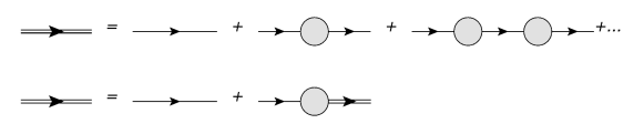
In order to derive the dressed fermionic propagator, we are going to use a system of self-consistent equations which involves the DS equation, Dyson’s series and the Ward-Takahashi identities. We will begin with the DS equation; it reads in real and momentum space, respectively:

$$\Sigma(x-y) = -ie^{2}\int d^{4}w\,\int d^{4}z\,{\cal G}(x-w)u^{\mu}G_{\mu\nu}(x-z)\Gamma^{\nu}(z;w,y),$$

$$\Sigma(p) = -ie^{2}{\int\!\frac{d^{4}k}{(2\pi)^{4}}\,}{\cal G}(p-k)u^{\mu}G_{\mu\nu}(k)\Gamma^{\nu}(k;p-k,p),$$ (7)

where $G_{\mu\nu}$ is the photon propagator, $\cal G$ is the fermion propagator and $\Gamma^{\mu}$ is the vertex function. The diagrammatic representation of equation (III.1) can be seen in Fig. 1. The DS equation describes the self-energy of the fermion. To obtain the full expression, we need to treat $\cal G$ as the exact fermion propagator and keep the photon propagator undressed (i.e. on tree-level), which coincides with the exact one in the framework of the BN model. The vertex correction is composed from both propagators but it can be simplified using the Ward-Takahashi relations, as we will see.

Figure 1: The diagrammatic representation of the Dyson-Schwinger equation. The double line is for the dressed fermion, the wavy line is for the photon propagator. The black blob denotes the full vertex function. The bold letters are for space-time points and the Greek letters denote the Lorentz indices. At finite temperatures we also need to consider the regular letters which are the Keldysh indices.

Now that we have the formula for the self-energy, we need another equation which expresses the fermion propagator as a function of the self-energy. For this purpose Dyson’s series can be used Pes . It can be shown that summing up all the radiative corrections to the free propagator will lead us to a sum of a geometric series (see Fig.  2). This results in an algebraic form:

$${\cal G}^{-1}(p)=Z(p-m)-\Sigma(p),$$ (8)

where we introduced $Z$ as the wave function renormalization factor coming from the vertex part. At this point we are not done yet, since in order to compute anything from (III.1) and (8) we would need an approximation of the vertex function $\Gamma^{\mu}$ to close the system of equations. However, in the case of the BN model we can relate the vertex correction to the fermion propagator in a unique way. This is the key point of the computation presented in JakoMati1 , and it can be achieved using the Ward-Takahashi identities. This exact equation is coming from the current conservation analogously to the QED case Pes ; itzy :

$$k_{\mu}\Gamma^{\mu}(k;p-k,p)={\cal G}^{-1}(p)-{\cal G}^{-1}(p-k).$$ (9)

In this model, however, the vertex function is proportional to $u^{\mu}$. In principle, the Lorentz-index in this model can come from $u^{\mu}$ or from any of the momenta. But, since the fermion propagator depends on the four-momentum in the form $u_{\mu}p^{\mu}$, the fermion-photon vertex does not depend on the momentum components which are orthogonal to $u^{\mu}$. Therefore the Lorentz-index which comes from $k^{\mu}$ in fact comes from the longitudinal part of $k^{\mu}$, i.e. proportional to $u^{\mu}$. So we can write $\Gamma^{\mu}(k;p-k,p)=u^{\mu}\Gamma(k;p-k,p)$. Using equations (III.1), (8) and (9) we can compute the exact fermion propagator. The detailed calculation can be found in JakoMati1 , where the Feynman gauge is used and the UV renormalization is performed systematically. This all boils down to the to the following differential equation:

$$(up-m){\cal G}^{\prime}+{\cal G}=-\frac{\alpha}{\pi}{\cal G},$$ (10)

and its solution is:

$${\cal G}(p)\propto(up-m)^{-1-\frac{\alpha}{\pi}}.$$ (11)

Figure 2: The diagrammatic representation of the Dyson’s series. The figure shows that the exact fermion propagator can be obtained as the sum of the radiative corrections. The double line represents the full fermion propagator, the grey blob is the self-energy which incorporates the radiative corrections. It can be shown that this sum is a geometric series and has the algebraic form of (8).

This is indeed the exact solution for the fermion propagator in the BN model BN . Comparing it to the free propagator, which has the form of $1/(up-m)$ the dressed solution has a power-law correction. This correction is due to the fully quantised soft radiation field, which shows in this respect that the electron cannot be thought as an independent object, but it is rather quasiparticle surrounded by the soft photon cloud. In the following we are going to give the solution for the finite temperature case.

III.2 The Bloch-Nordsieck model at $T>0$

In this section we will show the solution for the BN model at finite temperatures. There are a few studies on the finite temperature BN model with different approximations IancuBlaizot1 ; IancuBlaizot2 ; Weldon:1991eg ; Weldon:2003wp ; Fried:2008tb , however, the only analytically closed formula for the spectral function of the fermion is derived in JakoMati2 ; we will present the results from the latter. We already discussed that the $u^{\mu}$ parameter as the fixed four-velocity of the fermion implies that the Bloch-Nordsieck model describes the regime where the soft photon fields do not have energy even for changing the velocity of the fermion (no fermion recoil). This leads to the interpretation that the fermion is a hard probe of the soft photon fields, and as such it is not part of the thermal medium IancuBlaizot1 ; IancuBlaizot2 .
We are interested in the finite temperature fermion propagator. To determine it, we use the real time or Keldysh formalism (for details, see LeBellac ). Here the time variable runs over a contour containing forward and backward running sections ($C_{1}$ and $C_{2}$). The propagators are subject to boundary conditions which can be expressed as the KMS (Kubo-Martin-Schwinger) relations LeBellac . The physical time can be expressed through the contour time $t={\cal T}(\tau)$. This makes possible to work with fields living on a definite branch of the contour, $\Psi_{a}(t,{\bf x})=\Psi(\tau_{a},{\bf x})$ where ${\cal T}(\tau_{a})=t$, and $\tau_{a}\in C_{a}$ for $a=1,2$; and similarly for the gauge fields. The propagators are matrices in this notation, in particular the fermion and the photon propagator, respectively, reads as:

$$i{\cal G}_{ab}(x) = \left\langle{T_{\cal C}\Psi_{a}(x)\Psi_{b}^{\dagger}(0)}\right\rangle,$$

$$iG_{\mu\nu,ab}(x) = \left\langle{T_{\cal C}A_{\mu a}(x)A_{\nu b}(0)}\right\rangle,$$ (12)

where $T_{\cal C}$ denotes ordering with respect to the contour variable (contour time ordering). For a generic propagator $G_{11}$ corresponds to the Feynman propagator, and, since the $C_{2}$ contour times are always larger than the $C_{1}$ contour times, $G_{21}=G^{>}$ and $G_{12}=G^{<}$ are the Wightman functions. The KMS relation for a bosonic/fermionic propagator reads $G_{12}(t,{\bf x})=\pm G_{21}(t-i\beta,{\bf x})$ which has the following solution in Fourier space (with $k=(k^{0},{\bf k})$)

$$iG_{12}(k) = \pm n_{\pm}(k_{0})\varrho(k),$$

$$iG_{21}(k) = (1\pm n_{\pm})(k_{0})\varrho(k),$$ (13)

where

$$n_{\pm}(k_{0})=\frac{1}{e^{\beta k_{0}}\mp 1}\quad\mathrm{and}\quad\varrho(k)=iG_{21}(k)-iG_{12}(k)$$ (14)

are the distribution functions (Bose-Einstein (+) and Fermi-Dirac (-) statistics), and the spectral function, respectively. It is sometimes advantageous to change to the R/A formalism with field assignments $\Psi_{1,2}=\Psi_{r}\pm\Psi_{a}/2$. Then, one has $G_{aa}=0$ for both the fermion and the photon propagators. The relation between the propagators in the Keldysh formalism and the R/A propagators reads

$$G_{rr}=\frac{G_{21}+G_{12}}{2},\quad G_{11}=G_{ra}+G_{12},\quad\varrho=iG_{ra}-iG_{ar}.$$ (15)

The $G_{ra}$ propagator is the retarded, the $G_{ar}$ is the advanced propagator, $G_{rr}$ is usually called the Keldysh propagator in the framework of the R/A formalism (not to confuse with the propagators in the Keldysh formalism).

At zero temperature, as we could see in the previous section, the fermionic free Feynman propagator in the BN model has a single pole which means that there are no antiparticles in the model and it coincides with the retarded propagator of the theory. Consequently, all closed fermion loops are zero, thus there is no self-energy correction to the photon propagator at zero temperature, as we already discussed it. So, we will set ${\cal G}_{12}=0$, therefore the closed fermion loops as well as the photon self-energy remain zero even at finite temperature. Another, mathematical reason, why we must not consider dynamical fermions – which could show up in fermion loops – is that the spin-statistics theorem Pes forbids a one-component dynamical fermion field.
This means that now the exact photon propagator reads in Feynman gauge at finite temperature

$$G_{ab,\mu\nu}(k)=-g_{\mu\nu}G_{ab}(k),\\ G_{ra}=\frac{1}{k^{2}}\biggr{|}_{k_{0}\to k_{0}+i\varepsilon}.$$

And the exact photon spectral function is

$$\varrho(k)=2\pi\mathop{\textrm{sgn}}(k_{0})\delta(k^{2}).$$ (16)

All other propagators can be expressed using the identities in (III.2) and in (15).

Now we can consider the system of self-consistent equations at finite temperatures. The derivation of the DS equations at non-zero temperature can be found in JakoMati2 where the CTP (Closed Time Path) formalism was applied (see LeBellac ). Thus, one can express the equation for the fermion self-energy with the two-component notation as it can be seen in Fig. 1. In terms of analytic formulas it reads:

$$\Sigma_{ab}(x,y)=i\alpha_{a}e^{2}u_{\mu}\sum_{c,d=1}^{2}\int\!d^{4}wd^{4}z\,{\cal G}_{ac}(x,w)G^{\mu\nu}_{ad}(x,z)\Gamma_{\nu;dcb}(z;w,y),$$ (17)

where $\alpha_{a}=(-1)^{a+1}$. In Fourier space it is:

$$\Sigma_{ab}(p)=i\alpha_{a}e^{2}u_{\mu}\sum_{c,d=1}^{2}{\int\!\frac{d^{4}k}{(2\pi)^{4}}\,}{\cal G}_{ac}(p-k)G^{\mu\nu}_{ad}(k)\Gamma_{\nu;dcb}(k;p-k,p).$$ (18)

This equation is the non-zero temperature equivalent of (III.1), the only difference here is that, since we evaluate each operator on a given time contour, we need to indicate them, thus we use the lower indices for this purpose.
The vertex function in this case can be derived in a similar manner, too. The fact that the vertex function is proportional to $u^{\mu}$ is crucial again, in order to be able to apply the Ward-identities in a way we did already in the zero temperature computation. The derivation of Ward-identities at finite temperature is a straightforward generalisation of the formula that we have at zero temperature. It is easy to rewrite it in the two-component formalism, taking into account that to satisfy the delta functions requirement the time arguments must be on the same contour. One finds in Fourier space

$$k_{\mu}\Gamma^{\mu}_{abc}(k;p,q)=\left[\delta_{ab}{\cal G}_{bc}^{-1}(q)-\delta_{ac}{\cal G}_{bc}^{-1}(p)\right]\,(2\pi)^{4}\delta(k+p-q).$$ (19)

In the BN model, because of the special property of the vertex function, it is completely determined by the fermion propagator in the form:

$$\Gamma_{abc}(k;p,q)=\frac{1}{uk}\left[\delta_{ab}{\cal G}_{bc}^{-1}(q)-\delta_{ac}{\cal G}_{bc}^{-1}(p)\right]\biggr{|}_{p=q-k},$$ (20)

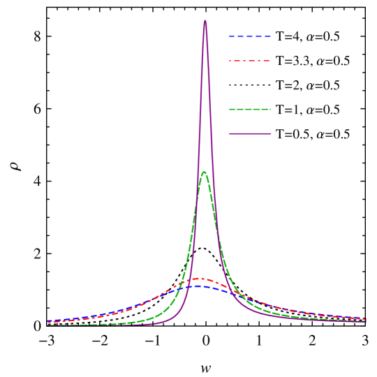
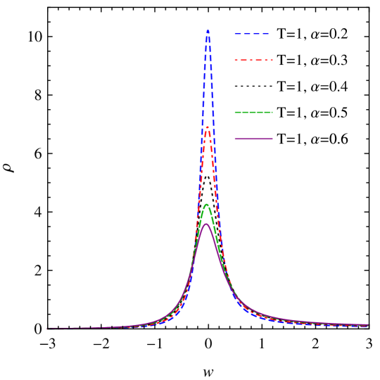
therefore the DS equations for the fermion propagator become closed. As the third component of the system of equations we will use (8) again. From (8), (18) and (20) the detailed calculation of the full solution can be found in JakoMati1 . At the end of the procedure we will get the following expression for the spectral function (defined as the discontinuity of the retarded propagator) in the special reference frame where $u=(1,0,0,0)$:

$$\rho(w)=\frac{\displaystyle N_{\alpha}\beta\sin\alpha\,e^{\beta w/2}}{\displaystyle\cosh(\beta w)-\cos\alpha}\,\frac{1}{\displaystyle\left|\Gamma\left(1+\frac{\alpha}{2\pi}+i\frac{\beta w}{2\pi}\right)\right|^{2}},$$ (21)

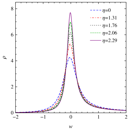
where $N_{\alpha}$ is an $\alpha$ dependent normalization factor, $\beta$ is the inverse temperature and $w=p_{0}-m$ is the variable (the energy shifted by the mass parameter). It can be shown that this result is completely consistent with the zero temperature one when one takes the $T\to 0$ limit JakoMati2 . In Fig. 3 we show the spectral function for different parameters of the temperature and the coupling constant $\alpha$. By increasing the temperature the broadening of the quasiparticle peak can be observed and the same effect can be achieved by increasing the coupling of the theory. The halfwidth of the curve can be related to the inverse of the lifetime of the quasiparticle; hence increasing the temperature lowers the lifetime of the quasiparticle which is physically sensible. The same can be said about varying the coupling constant. Since the Lorentz invariance does not hold at finite temperature we need to calculate the spectral function numerically when one goes from the rest frame of the fermion to a different one, for details see JakoMati2 . By increasing the four-velocity of the fermion the halfwidth shrinks, indicating more stable quasiparticles.

(a)

(b)

(c)

Figure 3: The fermionic spectral functions in the BN model at finite temperature. In (a) and (b) we see the broadening of the quasiparticle peak as the temperature and the coupling constant increased at fixed $\alpha=0.5$ and temperature $\beta=1/T=1$, respectively. In (c) the velocity dependence of the spectral function is shown for $\alpha=0.5$. The $\eta$ values are rapidities, $|{\bf{v}}|=\tanh\eta$. The peak region becomes sharper with increasing $\eta$ ($|{\bf{v}}|$).

The finite temperature fermion propagator can be retained using the spectral function in (21):

$${\mathcal{G}}(p)=\int\limits_{0}^{\infty}\frac{d\omega}{2\pi}\frac{\rho(\omega)}{p-\omega+i\epsilon}.$$ (22)

Since the $T\to 0$ limit of (21) gives back the spectral function that can be obtained for zero temperature (c.f. JakoMati1 ), this limit of the finite temperature propagator also gives back the $T=0$ formula (11) for this limit.

IV Applications

In this section we will present some of the ideas of the possible applications. As we have demonstrated that the soft photon contribution to the propagator of the electron is important both for $T=0$ and $T>0$ [(11) and (21)] we can use these expressions when we calculate processes in external fields. In such cases we can use the usual formula for the propagation in external field (see Fig. 4), except we use the propagator obtained from the BN model instead of the free one (both for $T=0$ and $T>0$):

$${\mathcal{G}}_{A}(x_{f},x_{i}) = {\mathcal{G}}(x_{f},x_{i})+\int d^{4}x_{1}{\mathcal{G}}(x_{f},x_{1})e\not{A}(x_{1}){\mathcal{G}}(x_{1},x_{i})$$ (23)

$$+\int\int d^{4}x_{1}d^{4}x_{2}{\mathcal{G}}(x_{f},x_{1})e\not{A}(x_{1}){\mathcal{G}}(x_{2},x_{1})e\not{A}(x_{2}){\mathcal{G}}(x_{2},x_{i})+...$$

Here we used ${\mathcal{G}}_{A}$ for the full propagator in the external field $A^{\mu}$ and ${\mathcal{G}}$ for the BN fermion propagator. Since we have a simpler form of the BN propagator in momentum space we should use for our calculations:

$${\mathcal{G}}_{A}(p_{f},p_{i}) = {\mathcal{G}}(p_{f})(2\pi)^{4}\delta^{4}(p_{f}-p_{i})+\int\,\frac{d^{4}p_{1}}{(2\pi)^{4}}{\mathcal{G}}(p_{f})e\not{A}(p_{1}){\mathcal{G}}(p_{i})$$ (24)

$$+\int\int\frac{d^{4}p_{1}}{(2\pi)^{4}}\,\frac{d^{4}p_{2}}{(2\pi)^{4}}\,{\mathcal{G}}(p_{f})e\not{A}(p_{1}){\mathcal{G}}(p_{i}+p_{2})e\not{A}(p_{2}){\mathcal{G}}(p_{i})(2\pi)^{4}\delta^{4}(p_{f}-p_{1}-p_{2}-p_{i})+...$$

In this expression $A^{\mu}$ can be considered as an arbitrary external field. For example we can use the Coulomb potential generated by a static point charge $-Ze$:

$$A_{0}(x)=-\frac{Ze}{|{\bf{x}}|},\qquad{\bf{A}}(x)={\bf{0}}.$$ (25)

Or in momentum space $A_{0}=-Ze4\pi/|{\bf q}|$. Alternatively, we can also use the screened Coulomb field: $A^{\mu}=-Ze\delta^{\mu\,0}/|{\bf{x}}|\exp(-|{\bf{x}}|/l)$, where $l$ is the screening length.

Figure 4: The BN propagator in the presence of an external field. The double line denotes the BN propagator, the letter ”X” is for the classical source producing the external field which are the wavy lines. The subscript $A$ on the left hand side denotes that the propagator is in the external field.

The interaction of the dressed electron with external field could have an application in the computation of processes like the multiphoton Compton scattering and the second order processes like the Bremsstrahlung, which are getting more important as the laser intensities are increasing. The main idea is similar to those of used in jent ; pia but instead of the Volkov propagator of the fermion the Bloch-Nordsieck propagator could be used.

V Summary

In this paper we discussed the infrared catastrophe in the framework of QED and its resolution using the Bloch- Nordsieck summation of radiative corrections. We sketched an alternative derivation of the Bloch-Nordsieck propagator with the aid of the Ward-identities; the full derivation is presented in JakoMati1 and for finite temperatures in JakoMati2 . The Bloch-Nordsieck propagator describes the propagation of the dressed electron in the deep infrared regime of the QED, where the soft photon contributions can be completely summed up. Speculation of the possible applications of the results are given in the last section. The detailed calculations of these processes are topic of current research projects.

VI Acknowledgement

The ELI-ALPS project (GOP-1.1.1-12/B-2012-0001) is supported by the European Union and co-financed by the European Regional Development Fund.

References

- (1) F. Bloch and A. Nordsieck, Phys. Rev. 52 (1937) 54.
- (2) M.E. Peskin, D.V. Schroeder, An Introduction to Quantum Field Theory, (Perseus Books Publishing, 1995).
- (3) C. Itzykson, J-B. Zuber, Quantum Field Theory, (McGraw-Hill Book Co., 1980)
- (4) H.M. Fried, Basics of Functional Methods and Eikonal Models (Atlantica Seguier Frontieres, 1990).
- (5) N.N. Bogoliubov and D.V. Shirkov, Introduction to the theories to the quantized fields (John Wiley & Sons, Inc., 1980).
- (6) A. Jakovac and P. Mati, Phys. Rev. D 85 085006 (2012), [arXiv:1112.3476 [hep-ph]].
- (7) A. Jakovac and P. Mati, Phys. Rev. D 87, 125007 (2013) [arXiv:1301.1803 [hep-th]].
- (8) J. -P. Blaizot and E. Iancu, Phys. Rev. D 55 (1997) 973 [hep-ph/9607303].
- (9) J. -P. Blaizot and E. Iancu, Phys. Rev. D 56, 7877 (1997) [hep-ph/9706397],
- (10) H. A. Weldon, Phys. Rev. D 44, 3955 (1991).
- (11) H. A. Weldon, Phys. Rev. D 69 (2004) 045006 [hep-ph/0309322].
- (12) H. M. Fried, T. Grandou and Y. -M. Sheu, Phys. Rev. D 77 (2008) 105027 [arXiv:0804.1591 [hep-th]].
- (13) N. P. Landsman and C. G. van Weert, Phys. Rept. 145, 141 (1987); M. Le Bellac, Thermal Field Theory, (Cambridge Univ. Press, 1996).
- (14) E. L tstedt, U. D. Jentschura and C. H. Keitel, Phys. Rev. Lett. 98, 043002 (2007).
- (15) F. Mackenroth, A. Di Piazza, Phys. Rev. A 83 032106 (2011).