A reaction diffusion-like formalism for plastic neural networks reveals dissipative solitons at criticality

Abstract

Self-organized structures in networks with spike-timing dependent plasticity (STDP) are likely to play a central role for information processing in the brain. In the present study we derive a reaction-diffusion-like formalism for plastic feed-forward networks of nonlinear rate neurons with a correlation sensitive learning rule inspired by and being qualitatively similar to STDP. After obtaining equations that describe the change of the spatial shape of the signal from layer to layer, we derive a criterion for the non-linearity necessary to obtain stable dynamics for arbitrary input. We classify the possible scenarios of signal evolution and find that close to the transition to the unstable regime meta-stable solutions appear. The form of these dissipative solitons is determined analytically and the evolution and interaction of several such coexistent objects is investigated.

Introduction

Activity in neuronal networks influences their coupling structure due to spike time-dependent synaptic plasticity (STDP) (Bi and Poo, 1998), which, in turn, influences the activity. Several works analytically investigated structures appearing in networks of neurons with plastic synapses under the influence of external signals. These studies required special network architectures, investigating e.g. a kind of possible ’elementary cell’ of the network (Nessler et al., 2013) or considered all-to-all connected networks (Galtier and Wainrib, 2012) or averages over activity realizations in space (Takeuchi and Amari, 1979) or systems without continuous spatial dimension (Gilson et al., 2009). Hebbian (Hebb, 1949) and similar learning rules, which can be considered as a simple STDP-like rules, are used in many neural network models, like e.g. Hopfield and Boltzmann networks (Chakrabarti and Basu, 2008). These works employ the energy minimization principle known in physics and set the values of synaptic weights according to the patterns to be stored, without considering the time evolution of the weights explicitly. These systems are able to store one level associations between patterns and recognize and restore externally applied and previously learned patterns. The memory capacity as well as times to recognize an input have been investigated (Chakrabarti and Basu, 2008). Activity propagation in non-plastic feed-forward systems was considered in (Gajic and Shea-Brown, 2013). A set of integro-differential equations, describing a spatially extended network, was introduced in (Wilson and Cowan, 1972) as the neural field model. A scheme of solution for a simplified version neglecting refractoriness (Amari, 1977) was later extended for neurons with adaptation (Coombes, 2005) and different non-linearities (Laing et al., 2002). The spatial and structural organization of cortex (Mountcastle, 1997; González-Burgos et al., 2000) separates different neural inputs either in real space or in an effective space that represents a continuum of features. For example, the orientation selectivity of neurons in visual cortex is represented by neurons topologically arranged on a one dimensional ring (Ben-Yishai et al., 1995). One suggested mechanism (Compte et al., 2000; Gutkin et al., 2001) to implement short-term memory is by localized bump solutions, which are also considered in (Laing et al., 2002). The latter work shows the relation between the formalism of reaction-diffusion-like systems and spatially extended non-plastic neural networks. Our work demonstrates such a relation for neural networks with long term plasticity. The formalism thus fills the gap between a series of studies of plastic networks without spatial dimension and the formalism describing activity in spatially extended networks. The presented analysis therefore opens the possibility to study the transfer of short-term memory, encoded by bump solutions, into long-term memory, stored by synaptic modifications. Here we analytically consider a feed-forward network with space-dependent connectivity and linear-non-linear neurons with a simple STDP-inspired synaptic learning rule, similar to the BCM rule (Bienenstock et al., 1982). We reduce the discrete problem by diffusion approximation to obtain an equation similar but not exactly equivalent to a reaction-diffusion equation with one component, also called Kolmogorov-Petrovsky-Piskounov equation (Kolmogorov et al., 1937; Liehr, 2013). We derive the requirements on the non-linearity necessary for a regime of stable signal propagation, exposing that fine-tuning of parameters is necessary, explaining earlier results (Kunkel et al., 2011). The bump solutions that are stable in the critical and meta-stable in the subcritical regime are described analytically. The interneural connections inside a bump are strengthened, resembling cell assemblies (Vogels et al., 2011) and showing how externally presented objects (external input) change intrinsic system properties (connectivity).

We further consider the interaction between bump solutions in dependence of their size, the distance between them, and the system parameters. In the regime close to stable propagation we find that several coexisting activity bumps can either unite with each other or remain disjoint, depending on the initial conditions. Their unification can be interpreted as an emergence of connections between cell-assemblies, and, in this way, represents a system of associations between internal representations of corresponding external stimuli. The improved formalism can be generalized to neural networks with several neuron types and to some extent mapped onto the time evolution of a recurrent network, opening the possibility for further investigations.

Results

Model definition

Here we consider feed forward networks consisting of $M$ layers of $N$ neurons each. A neuron at position $\tilde{x}$ in layer $n+1$ gets as input $u_{\tilde{x}}$ the weighted sum of outputs $r$ of an odd number $K$ of neurons from the neighborhood in the previous layer $n$, $u_{\tilde{x}}=\sum_{x=\tilde{x}-(K-1)/2}^{x=\tilde{x}+(K-1)/2}w_{\tilde{x}x}r_{x}$, where the indices $\tilde{x}$ and $x$ describe the positions of the postsynaptic neuron in the layer $n+1$, and of the presynaptic neuron in the layer $n$, respectively. Here $w_{\tilde{x}x}$ is the synaptic weight from neuron $x$ to neuron $\tilde{x}.$ The neuron’s output $r=f(u)$ is its input $u$ mapped by the non-linear function $f$. This network architecture is illustrated in Figure 1. The absence of feedback allows the solution of the system, finding the activities and synaptic weights for each pair of layers separately using the solution of the previous pair as an input.

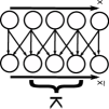
Figure 1: Two neighboring layers in the considered feed-forward architecture. Synapses between layers obey the plasticity rule (1).

We assume a Hebbian plasticity rule

$$\dot{w}_{\tilde{x}x}=-\alpha(w_{\tilde{x}x}-w_{0})+\gamma r_{x}r_{\tilde{x}}$$ (1)

for the presynaptic neuron $x$ and the postsynaptic neuron $\tilde{x}$, which is similar to the BCM rule (Bienenstock et al., 1982), but without the “sliding” threshold in the non-linearity $f$. As a result, the function $f$ keeps its sign. For simulations we used $f(x)=A/(1+e^{-\beta(x-\theta)})-A/(1+e^{\beta\theta})$. If a stationary solution exists it can be found requiring $\dot{w}_{\tilde{x}x}=0$ as

$$w_{\tilde{x}x} = w_{0}+\frac{\gamma}{\alpha}r_{x}r_{\tilde{x}}=w_{0}+\frac{\gamma}{\alpha}f(u_{x})f(u{}_{\tilde{x}}).$$ (2)

In the following we use $\xi=u_{\tilde{x}}$ as the summed input to the postsynaptic neuron to better distinguish it from the presynaptic neuron’s $u$.

In equilibrium, after the learning processes stopped, $\xi$ is to be found as a solution of the self-consistent equation

$$\xi_{\tilde{x}} = \check{f}(r_{\xi})=\sum_{x=\tilde{x}-(K-1)/2}^{\tilde{x}+(K-1)/2}w_{\tilde{x}x}r_{x}$$

$$\stackrel{{\scriptstyle(\ref{eq:w_stationary})}}{{=}} w_{0}\sum_{x=\tilde{x}-(K-1)/2}^{\tilde{x}+(K-1)/2}r_{x}+\frac{\gamma}{\alpha}f(\xi)\sum_{x=\tilde{x}-(K-1)/2}^{\tilde{x}+(K-1)/2}r_{x}^{2},$$

with $r_{\xi}=f(\xi)$ and the symbol $\check{}$ denoting the inverse function. In the approximation neglecting further derivatives (and being exact for $K=3$ and $\partial_{x}$ denoting the discrete lattice derivative) one can replace $\sum_{x=\tilde{x}-(K-1)/2}^{\tilde{x}+(K-1)/2}$ with $(K+a\partial_{x}^{2})$ where $a=\sum_{n=0}^{(K-1)/2}n^{2}=(K-1)K(K+1)/24$. In doing so, we also make the transition from a discrete index $x$ to a continuous variable, also denoted as $x$. So, processes in the system can be considered as an interplay between the diffusion described by the $\partial_{x}^{2}$-operator and the explicit (given by $f$) and implicit non-linearities, due to the term $r_{x}^{2}$ in (Model definition) resulting from plasticity. The equation (Model definition) can be rewritten in this approximation as

$$\xi=\check{f}(r_{\xi})=w_{0}(K+a\partial_{x}^{2})r+\frac{\gamma}{\alpha}r_{\xi}(K+a\partial_{x}^{2})r^{2}.$$ (4)

Analysis of global stability and self-reproducing solutions

One can search for possible stable solutions $\xi(x)=u(x)$, satisfying

$$\check{f}(r)=w_{0}(K+a\partial_{x}^{2})r+\frac{\gamma}{\alpha}r(K+a\partial_{x}^{2})r^{2},$$ (5)

where $r(x)=f(u(x))$. There are no terms explicitly depending on the variable $x$, so one can reduce the order of the equation by introducing $y(r)=[\partial_{x}r](r)$ the derivative of $r$ depending on $r$. We can hence express the second derivatives in (5) as

$$\partial_{x}^{2}r = \partial_{x}y=\partial_{r}y\,\partial_{x}r=y\,\partial_{r}y$$ (6)

$$\partial_{x}^{2}(r^{2}) = 2(\partial_{x}r)^{2}+2r\,\partial_{x}^{2}r=2y^{2}+2ry\,\partial_{r}y=2z+r\,\partial_{r}z,$$

where we used the substitution $z(r)=y^{2}=(\partial_{x}r)^{2}$ in the last step. Eq. (5) then takes the form of a linear differential equation in $z$

$$\check{f}(r) = w_{0}(K\,r+a\,y\,\partial_{r}y)+\frac{\gamma}{\alpha}(r^{3}K+ar\,(2z+r\,\partial_{r}z))$$

$$= w_{0}K\,r+\frac{\gamma}{\alpha}r^{3}K+2\frac{\gamma}{\alpha}ar\,z+(\frac{1}{2}w_{0}a+\frac{\gamma}{\alpha}ar^{2})\,\partial_{r}z,$$

replacing $y\,\partial_{r}y$ in the first line with $\frac{1}{2}\partial_{r}z$ in the second line. The solution of the corresponding homogeneous equation $2\frac{\gamma}{\alpha}arz+(\frac{1}{2}w_{0}a+\frac{\gamma}{\alpha}ar^{2})\,\partial_{r}z=0$ is $H(r)=\exp(-\intop^{r}\frac{2\frac{\gamma}{\alpha}ar^{\prime}}{\frac{1}{2}w_{0}a+\frac{\gamma}{\alpha}ar^{\prime 2}}\,dr^{\prime})=c\,\exp(-\ln(\frac{1}{2}w_{0}a+\frac{\gamma}{\alpha}ar^{2}))=c\frac{2}{a(w_{0}+2\frac{\gamma}{\alpha}r^{2})}$ (with an arbitrary constant $c$), and as solution of (Analysis of global stability and self-reproducing solutions) one gets

$$z(r)=\frac{2}{a(w_{0}+2\frac{\gamma}{\alpha}r^{2})}\int^{r}\underbrace{\left(\check{f}(r^{\prime})-K(w_{0}+\frac{\gamma}{\alpha}r^{\prime 2})r^{\prime}\right)}_{\equiv q(r^{\prime})}\,dr^{\prime},$$ (8)

where we used that the factor in front of $\partial_{r}z$ cancels with $H^{-1}$. As $z$ is the square of a real number and hence cannot be negative, a solution existing for all $r$ (starting from $r=0$) has to satisfy $Q(r)=\int_{0}^{r}q(r^{\prime})\,dr^{\prime}\geq 0$. We are seeking for solutions that start at $r=0$. We call $r_{\mathrm{max}}$ the largest value of $r$ reached, for which $\partial_{x}r=0$ and therefore $z(r_{\mathrm{max}})=0$ from which follows

$$Q(r_{\mathrm{max}}) = 0.$$ (9)

For this case $Q(r)$, $q(r)$ and the stable solution $r(x)$ are shown in Figure 2. The physical meaning of $q(r)$ is the competition between the non-linearity $f$ and the effective non-linearity $K(w_{0}+\frac{\gamma}{\alpha}r^{2})r$ that describe the propagation of $r$ neglecting diffusion: $K(w_{0}+\frac{\gamma}{\alpha}r^{2})r$ is the value of a postsynaptic neuron’s membrane potential $\xi$ for the case that presynaptic and postsynaptic neurons have $u=\check{f}(r)$. So, a positive $q(r)$ indicates a decrease of $u$ and $r$ from one layer to the next, and negative $q(r)$ corresponds to both measures increasing. So, in a stable system we must have $Q(r)\geq 0$ for all $r\geq 0$. By definition, $Q(r)=0$ for $r=0$. If there are no other $r$ at which $Q(r)=0$, there exists no self-consistent solution propagating from layer to layer without change. If one tries to construct the stable solution according to (8) for this case, one will always have positive $\partial_{x}r$ for every $r>0$, which means that for every $r>0$ ’external support’ is needed to compensate the diffusion effects, and without it every finite signal will decay after some layers. For the case of the presence of an $r$ with $Q(r)=0$, a solution exists having this $r$ as the maximum. If $q(r)=\partial_{r}Q(r)$ at that point is negative, an arbitrary small positive perturbation added to this maximum $r$ will grow. So, $Q(r)<0$ for some $r$ means the absence of a stable solution and explosion of activity for sufficiently strong activation patterns.

The solution is given in the form $z(r)=(\partial_{x}r)^{2}$, where the choice of a positive or negative sign in taking the square root corresponds to a solution that is first increasing or decreasing, respectively, when moving from left to right. The length of a “plateau” with $\partial_{x}r=0$ and $Q(r_{\mathrm{max}})=0$ is an arbitrary parameter of the solution which can be chosen freely. If two such solutions coexists, they lead to the growth of $r$ in the region between borders of their plateaus and to their junction to one without the external borders changing.

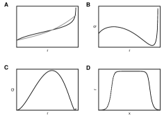
Figure 2: A Explicit $\check{f}(r)$ (black) and implicit $K(w_{0}+\frac{\gamma}{\alpha}r^{2})r$ non-linearity (gray). B Their difference, $q(r)$. C $Q(r)=\int q(r)dr$, a minimum of $Q$ of $0$ enables a stable non-trivial solution $r(x)$ shown in D - theoretical prediction of the stable solution with dashed line and simulation results with solid line. Simulation parameters: $N=800$, $M=400$, $K=41$, $w_{0}=0.99/K$, $\gamma=0.99/K$, $\theta=0.6$, $\beta=3.6$, $A=1.0754$.

The form of the rest of the bump - the left and right wings $r=p(x)$ - is independent of the plateau’s width and can be obtained from (8) analytically or by numerical integration as the inverse function of $\check{p}(r)=\int^{r}\pm 1/\sqrt{z}\,dr=\int^{r}\pm 1/\sqrt{\frac{2}{a(w_{0}+2\frac{\gamma}{\alpha}r^{2})}Q(r)}\,dr$ integrating from an arbitrary value of $r$ between $0$ and $r_{\mathrm{max}}$ and taking plus for the left or minus for the right wing.

Long-living solutions in sub-critical regime

If no $r_{\mathrm{max}}>0$ with $Q(r_{\mathrm{max}})=0$ exists, but $Q(\tilde{r}_{\mathrm{max}})$ has a local minimum close to zero, one gets similar structures as the “immortal” solutions for (9). The bump solutions propagate over large but finite numbers of layers before they disappear. This number is approximately proportional to the initial width $S$ of the plateau: for $S$ larger than $K$, the successive reduction of this width does not affect the processes on the borders, and the velocity $s$, i.e.the rate of reduction of the plateau’s width from layer to layer, is approximately constant, depending only on network parameters as shown in Figure 3. The velocity $s$ can be calculated as the propagation speed that makes the solution stable. Obtaining the rate profile for the previous layer as a slightly shifted version $r(x)-s\partial_{x}r(x)$ of the profile $r(x)$ in the current layer one obtains from (4)

$$\check{f}(r)=w_{0}(K+a\partial_{x}^{2})(r-s\partial_{x}r)+\frac{\gamma}{\alpha}r(K+a\partial_{x}^{2})(r-s\partial_{x}r)^{2}$$

or, after sorting, neglecting terms $O(s^{2})$, using the definition of $q(r)$ in (8) and multiplying with $\partial_{x}r$

$$q(r)\partial_{x}r-sw_{0}K(\partial_{x}r)^{2}-sw_{0}a\partial_{x}^{3}r\,\partial_{x}r+aw_{0}\partial_{x}^{2}r\,\partial_{x}r=$$

$$-2s\frac{\gamma}{\alpha}Kr^{2}(\partial_{x}r)^{2}+\frac{\gamma}{\alpha}ar\partial_{x}r\partial_{x}^{2}(r^{2})-2s\frac{\gamma}{\alpha}ar\partial_{x}^{2}(r\partial_{x}r)\partial_{x}r$$

which, after integrating over $x$ from minus infinity to the beginning of the plateau, leads to

$$Q(\tilde{r}_{\mathrm{max}}) = -s\int_{0}^{\tilde{r}{}_{\mathrm{max}}}w_{0}K\partial_{x}r+aw_{0}\partial_{x}^{3}r+\frac{\gamma}{\alpha}(2Kr^{2}\partial_{x}r$$ (10)

$$+ 2ar\partial_{x}^{2}(r\partial_{x}r)+ar\partial_{x}^{2}(r^{2}))+aw_{0}\partial_{x}^{2}r\,dr.$$

The last two terms in the latter expression vanish, because $\int_{0}^{\tilde{r}{}_{\mathrm{max}}}\partial_{x}^{2}r\ dr=\int_{0}^{\tilde{r}{}_{\mathrm{max}}}y\partial_{r}y\ dr=\frac{1}{2}(\partial_{x}r)^{2}|_{r=0}^{r=\tilde{r}{}_{\mathrm{max}}}=0$. Further we have $\int_{0}^{\tilde{r}{}_{\mathrm{max}}}r\partial_{x}^{2}(r^{2})\ dr=\frac{1}{2}\int_{0}^{\tilde{r}{}_{\mathrm{max}}^{2}}\partial_{x}^{2}(r^{2})\ dr^{2}=\frac{1}{2}\int_{0}^{\tilde{r}^{2}{}_{\mathrm{max}}}y_{2}\partial_{r^{2}}y_{2}\ dr^{2}=\frac{1}{4}(\partial_{x}(r^{2}))^{2}|_{r=0}^{r=\tilde{r}{}_{\mathrm{max}}}=0$ with $y_{2}=[\partial_{x}(r^{2})](r^{2})$ similar to $y(r)=[\partial_{x}r](r)$, because $\tilde{r}{}_{\mathrm{max}}$ is the plateau height and derivatives of $r$-dependent functions are $0$. One can therefore obtain $s$ with

$$s = -Q(\tilde{r}_{\mathrm{max}})/(\int_{0}^{\tilde{r}_{max}}(w_{0}K\partial_{x}r+2\frac{\gamma}{\alpha}Kr^{2}\partial_{x}r+$$ (11)

$$2\frac{\gamma}{\alpha}ar\partial_{x}^{2}(r\partial_{x}r)+aw_{0}\partial_{x}^{3}r)\,dr).$$

One can replace $\partial_{x}r$ with the dependence $\partial_{x}r=\sqrt{z(r)}$ given by (8) obtained for $Q(\tilde{r}{}_{\mathrm{max}})=0$ - this approximation is meaningful for integrative quantities that are not influenced strongly by the local variation of $Q$ near $\tilde{r}_{\mathrm{max}}$. The chain rule allows the replacement of $\partial_{x}$ with $\partial_{x}r\partial_{r}$, in this way one can express $s$ in terms of the integral of the function containing $z(r)$ over $r$.

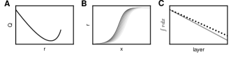
Figure 3: A $Q(r)$ near its minimum close to but bigger than $0$. B Rate profiles $r(x)$ in different layers showing the reduction of the plateau’s width for a long-living rate profile leading to linear decrease with the layer’s number of $\int r(x)\,dx$. C The theoretical expectation (11) and the simulated result for $\int r(x)\,dx$. Parameters as for Figure 2 apart from $A=1.0745$.

To understand how the system represents two or more coexistent signals, we investigate the situation with two coexistent meta-stable solutions. Two such bumps can unite into one if the minimal amplitude of $r$ between their borders becomes big enough for self-generated growth before one of the plateaus disappears.

Without loss of generality we take $x=0$ for the midpoint between the bumps. If the distance between the two closer ends of the bumps’ plateaus is larger than some critical value, the minimal $r=r_{\mathrm{min}}$ at the minimum position $x=0$ decays. One can roughly estimate the change $\delta r_{\mathrm{min}}$ of $r_{\mathrm{min}}$ from one layer to the next, approximating $r(x)$ near $x=0$ with the direct sum of the two bumps’ wings, i.e. $r=p(x+\check{p}(r_{\mathrm{min}}/2))+p(-x+\check{p}(r_{\mathrm{min}}/2))$ with $p(x)$ denoting a wing of a bump with $p(0)=\tilde{r}_{\mathrm{max}}$ at the plateau’s edge. The factor $1/2$ appears because the direct sum of two identical bump solutions approximately produce the value $r_{\mathrm{min}}$. In this approximation $\delta r_{\mathrm{min}}(r_{\mathrm{min}})=r_{\mathrm{min}}^{new}(r_{\mathrm{min}})-r_{\mathrm{min}}$, where $r_{\mathrm{min}}^{new}=f([w_{0}(K+a\partial_{x}^{2})r+r(K+a\partial_{x}^{2})r^{2}]|_{x=0})$. $\delta r_{\mathrm{min}}(r_{\mathrm{min}})$ is shown in Figure 4. The critical distance is given by $\check{p}(r_{\mathrm{min}}^{\mathrm{crit}}/2),\ \delta r_{\mathrm{min}}(r_{\mathrm{min}}^{\mathrm{crit}})=0$. For larger distances no direct unification of two bumps is possible independent of their plateau widths.

The “next generation” of bumps resulting from this merging can interact in the same way with each other and the bumps of previous generations that are still alive. In this way an association tree reflecting the input structure can be created as illustrated in Figure 4.

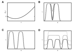
Figure 4: A Theoretical prediction of the change of minimal activity $r_{\mathrm{min}}$ between bumps after one layer. B Propagation of two bumps uniting to one, in C they remain disjoint, because their initial distance exceeds the maximal distance for unification. D Rate profiles in three layers. The activity of the bumps is shifted upwards in proportion to the layer number for clearer distinction. The evolution over layers illustrates the construction of an ’association tree’: first the left and the middle bumps are joint, and later the right one. Parameters as for Figure 3 apart from $\gamma=0$, $w_{0}=1.4/K$, $\beta=3.63$ for panels A-C.

Discussion

We obtain equations describing the propagation of activity from layer to layer in feed-forward networks of nonlinear rate neurons with an STDP-inspired plasticity rule. We find that the stability of the considered network is determined by the sign of the minimum of the function $Q(r)$: for positive sign, every perturbation decays, for negative sign activity explodes for any sufficiently strong perturbation. If the minimum is $0$, stable attractive solutions exist. They have an analytically obtained form containing a plateau of variable width. So, precise tuning of parameters is required to get stable propagation of activity patterns unchanged from layer to layer, in agreement with earlier simulation results of (Kunkel et al., 2011). A sigmoidal form of the nonlinearity $f$ can help to get an alteration of the signs of $q=\partial_{r}Q(r)$, necessary to ensure the existence of a minimum of $Q(r)=0$ at a non-vanishing activity level $r>0$. A sigmoidal $f$ is therefore a natural choice to bring the system close to criticality. The qualitative form of the gain function found here is in line with the sigmoidal form derived in (Han and Koh, 1999) for feed-forward classification networks. The argumentation and the network model of this earlier work are, however, quite different. Their model does not include spatial organization. Rather, the authors find the sigmoid resulting from the requirement of optimal stability in the recognition of presented and previously learned patterns, without investigating the learning process itself. For the latter they employ the known error backpropagation mechanism, fixing the synaptic weights prior to the consideration of the neuronal activation dynamics. Employing field theoretic arguments, the sigmoid is found as a soliton (kink) solution, where the input strength to the nonlinearity plays the role of space. The dissipative soliton solutions in our work, in contrast, are solutions in real space. Similar long-living bump solutions exist in systems with positive minima of $Q(r)$ close to $0$. These solutions decay with a velocity increasing with the value of this minimum. Two bumps can unite if the interplay of diffusion and nonlinearity between them overcomes the decay when propagating from one layer to the next; otherwise they remain disjoint. For a united bump the same scenarios exist, so a kind of association tree can appear in this way. Qualitatively, all interesting results presented in this article do not require the existence of the correlation sensitive term ($\gamma\neq 0$) and exist also in the system with static synapses, for which the correspondence to differential equations is known (Laing et al., 2002). For $\gamma=0$ (5) is rewritten as $q(r)=aw_{0}\partial_{x}^{2}r$, describing the stable solution of a reaction-diffusion equation (RDE) for one chemical with the reaction nonlinearity $q$ and diffusion coefficient $aw_{0}$. One can also interpret the layers in the network as different states of the system evolution in time on a discretized time grid. The corresponding time-continuous equation $\partial_{t}u=aw_{0}\partial_{x}^{2}r-q(r)$ with redefined $q(r)=\check{f}(r^{\prime})/\tau_{m}-Kw_{0}r$ for the presence of a linear leak $-u/\tau_{m}$ is analog to a RDE for the time evolution of a system with one chemical. Dissipative solitons are known to be solutions of such systems (Liehr, 2013) and correspond to the bump solutions (8). The interesting and non-trivial result is, that such solutions exist also for arbitrary learning rates $\gamma\neq 0$ and that their shape can be obtained analytically.

A more general equation $q(r)=\sum_{i}D_{i}(r)\partial_{x}^{2}F_{i}(r)$ of the same type as (5), but with an arbitrary number of functions under the second derivative is solved with the same substitutions $z,\ y$: $q(r)=\sum_{i}D_{i}(r)\partial_{x}^{2}F_{i}(r)=\sum_{i}D_{i}(r)((\partial_{x}^{2}r)\partial_{r}F_{i}(r)+(\partial_{x}r)^{2}\partial_{r}^{2}F_{i}(r))=\frac{1}{2}(\sum_{i}D_{i}(r)\partial_{r}F_{i}(r))\partial_{r}z+(\sum_{i}D_{i}(r)\partial_{r}^{2}F_{i}(r))z$, $z(r)=2H(r)\int H^{-1}(r^{\prime})\frac{q(r^{\prime})}{\sum_{i}D_{i}(r^{\prime})\partial_{r^{\prime}}F_{i}(r^{\prime})}\ dr^{\prime}$ with $H(r)=\exp(-2\intop^{r}\frac{\sum_{i}D_{i}(r^{\prime})\partial_{r^{\prime}}^{2}F_{i}(r^{\prime})}{\sum_{i}D_{i}(r^{\prime})\partial_{r^{\prime}}F_{i}(r^{\prime})}\,dr^{\prime})$. Further simplifications done for (8) were applicable only to this particular problem and are impossible in the general case. This generalized equation can be used to describe e.g. stable solutions for systems with several neuron and synapse types, in particular networks including inhibitory neurons. There the interaction between several bumps can exhibit more complex behavior than in the case of non-plastic synapses (Laing et al., 2002). This equation is similar but not equivalent to an equation describing a one-component reaction-diffusion system (for only one $i$ this mapping is exact). Still, a similar analysis of the existence of stable and meta-stable solutions, as presented for (5), is possible for this more general case. Preliminary results indicate that associative learning and memory can persist even if the activity is restored to the baseline level, similar as in (Vogels et al., 2011). In contrast to classical models of associative memory, such as fully connected Hopfield networks and Boltzmann machines (Chakrabarti and Basu, 2008), our formalism allows the study of spatially extended representations of earlier presented, learned objects.

With the leak term $-u/\tau_{m}$, the evolution of activity is described by $\partial_{t}u_{t}(\tilde{x})=-\tau_{m}^{-1}u_{t}(\tilde{x})+\sum_{x=\tilde{x}-(K-1)/2,\ x\neq\tilde{x}}^{\tilde{x}+(K-1)/2}w_{t}(\tilde{x},x)r_{t}(x),$ for stationary solutions $u(\tilde{x})=\sum_{x=\tilde{x}-(K-1)/2,\ x\neq\tilde{x}}^{\tilde{x}+(K-1)/2}\tau\,[w_{0}+\frac{\gamma}{\alpha}f(u(x))f(u(\tilde{x}))]f(u(x))$, which, after diffusion approximation of the sum, is equivalent to (5) with parameters $\tau\gamma$, $\tau w_{0}$ and $K-1$ instead of $\gamma$, $w_{0}$ and $K$. So the presented results generalize to stationary solutions in recurrent networks.

References

- Bi and Poo (1998) G. Bi and M. Poo, J. Neurosci. 18, 10464 (1998).
- Nessler et al. (2013) B. Nessler, M. Pfeiffer, L. Buesing, and W. Maass, PLOS Comput. Biol. 9, e1003037 (2013).
- Galtier and Wainrib (2012) M. Galtier and G. Wainrib, Journal of MAthematical Neuroscience 2, 13 (2012).
- Takeuchi and Amari (1979) A. Takeuchi and S. Amari, Biol. Cibern. 35, 63 (1979).
- Gilson et al. (2009) M. Gilson, A. N. Burkitt, D. B. Grayden, D. A. Thomas, and J. L. van Hemmen, Biol. Cybern. 101, 81 (2009).
- Hebb (1949) D. O. Hebb, The organization of behavior: A neuropsychological theory (John Wiley & Sons, New York, 1949).
- Chakrabarti and Basu (2008) B. K. Chakrabarti and A. Basu, Neural network modeling, vol. 168 (2008).
- Gajic and Shea-Brown (2013) N. C. Gajic and E. Shea-Brown, Neural Computation 25 (2013).
- Wilson and Cowan (1972) H. R. Wilson and J. D. Cowan, Biophys. J. 12, 1 (1972).
- Amari (1977) S.-i. Amari, Biol. Cybern. 27, 77 (1977).
- Coombes (2005) S. Coombes, Biol. Cybern. 93, 91 (2005).
- Laing et al. (2002) C. R. Laing, W. C. Troy, B. Gutkin, and B. G. Ermentrout, SIAM J. Appl. Math. 63, 62 (2002).
- Mountcastle (1997) V. B. Mountcastle, Brain 120, 701 (1997).
- González-Burgos et al. (2000) G. González-Burgos, G. Barrionuevo, and D. A. Lewis, Cereb. Cortex 10, 82 (2000).
- Ben-Yishai et al. (1995) R. Ben-Yishai, R. Bar-Or, and H. Sompolinsky, Proc. Nat. Acad. Sci. USA 92, 3844 (1995).
- Compte et al. (2000) A. Compte, N. Brunel, P. S. Goldman-Rakic, and X. J. Wang, Cereb. Cortex 10, 910 (2000).
- Gutkin et al. (2001) B. Gutkin, C. R. Laing, C. L. Colby, C. Chow, and G. Ermentrout, J. Comput. Neurosci. 11, 121 (2001).
- Bienenstock et al. (1982) E. L. Bienenstock, L. N. Cooper, and P. W. Munro, J. Neurosci. 2, 32 (1982).
- Kolmogorov et al. (1937) A. Kolmogorov, I. Petrovsky, and N. Piscounov, Moscow Univ. Bull. Math. 1, 1 (1937).
- Liehr (2013) A. W. Liehr, Dissipative Solitons in Reaction Diffusion Systems (Springer-Verlag, 2013), ISBN 978-3-642-31250-2.
- Kunkel et al. (2011) S. Kunkel, M. Diesmann, and A. Morrison, Front. Comput. Neurosci. 4 (2011).
- Vogels et al. (2011) T. Vogels, H. Sprekeler, F. Zenke, C. Clopath, and W. Gerstner, Science 334, 1569 (2011).
- Han and Koh (1999) S.-H. Han and I. G. Koh, Physical Review E 60, 7608 (1999).