Tau-REx II: Retrieval of emission spectra

Abstract

$\mathcal{T}$-REx (Tau Retrieval of Exoplanets) is a novel, fully Bayesian atmospheric retrieval code custom built for extrasolar atmospheres. In Waldmann et al. (2015) the transmission spectroscopic case was introduced, here we present the emission spectroscopy spectral retrieval for the $\mathcal{T}$-REx framework. Compared to transmission spectroscopy, the emission case is often significantly more degenerate due to the need to retrieve the full atmospheric temperature-pressure (TP) profile. This is particularly true in the case of current measurements of exoplanetary atmospheres, which are either of low signal-to-noise, low spectral resolution or both. Here we present a new way of combining two existing approaches to the modelling of the said TP profile: 1) the parametric profile, where the atmospheric TP structure is analytically approximated by a few model parameters, 2) the Layer-by-Layer approach, where individual atmospheric layers are modelled. Both these approaches have distinct advantages and disadvantages in terms of convergence properties and potential model biases. The $\mathcal{T}$-REx hybrid model presented here is a new two-stage TP profile retrieval, which combines the robustness of the analytic solution with the accuracy of the Layer-by-Layer approach. The retrieval process is demonstrated using simulations of the hot-Jupiter WASP-76b and the hot SuperEarth 55 Cnc e, as well as on the secondary eclipse measurements of HD189733b.

1 Introduction

The characterisation of extrasolar planets through the spectroscopic measurements of their atmospheres has become a well established field today (Tinetti et al. 2013). In Waldmann et al. (2015), we presented the $\mathcal{T}$-REx (Tau Retrieval of Exoplanets) suite for transmission spectroscopic measurements. In this paper we introduce the corresponding retrieval for emission spectroscopic data.

Transmission and emission spectroscopy carry highly complementary aspects. Whereas transmission spectroscopy is less sensitive to thermal gradients, the emission spectroscopy case probes the full temperature-pressure profile (TP-profile hereafter) of the atmosphere. This makes the emission case significantly harder to constrain without the luxury of in-situ measurements. King (1958) was the first to suggest remote sensing of the planetary atmospheric temperature structure through the infra-red, thermal radiance of the planet. Kaplan (1959) expanded on this pioneering work by laying the foundations of retrieving exact TP-profiles from emission spectroscopic measurements. Remote sensing of planetary atmospheres in our solar system has been a long story of success (e.g. Wark & Hilleary 1969; Conrath et al. 1970; Hanel et al. 1972; Conrath et al. 1973; Rodgers 1976; Hanel et al. 1981; Fletcher et al. 2007; Irwin et al. 2008) as well as Hanel et al. (2003), and references therein. More recently, emission spectroscopy remote sensing has been expanded to exoplanetary atmospheres (Madhusudhan & Seager 2009; Lee et al. 2011; Line et al. 2012; Griffith 2014). Line et al. (2013) provides a comparison of existing exoplanetary emission spectroscopy retrieval codes.

1.1 $\mathcal{T}$-REx

$\mathcal{T}$-REx  is a novel, Bayesian atmospheric spectroscopy retrieval suite designed for extrasolar planets. In Waldmann et al. (2015), hereafter W15, we introduce the overall architecture, data handling, minimisation/sampling routines, handling of molecular line lists, Bayesian model selection and the transmission spectroscopy forward model. In this publication we present the emission spectroscopy forward model as well as the atmospheric temperature-pressure (TP) profile retrieval implemented.

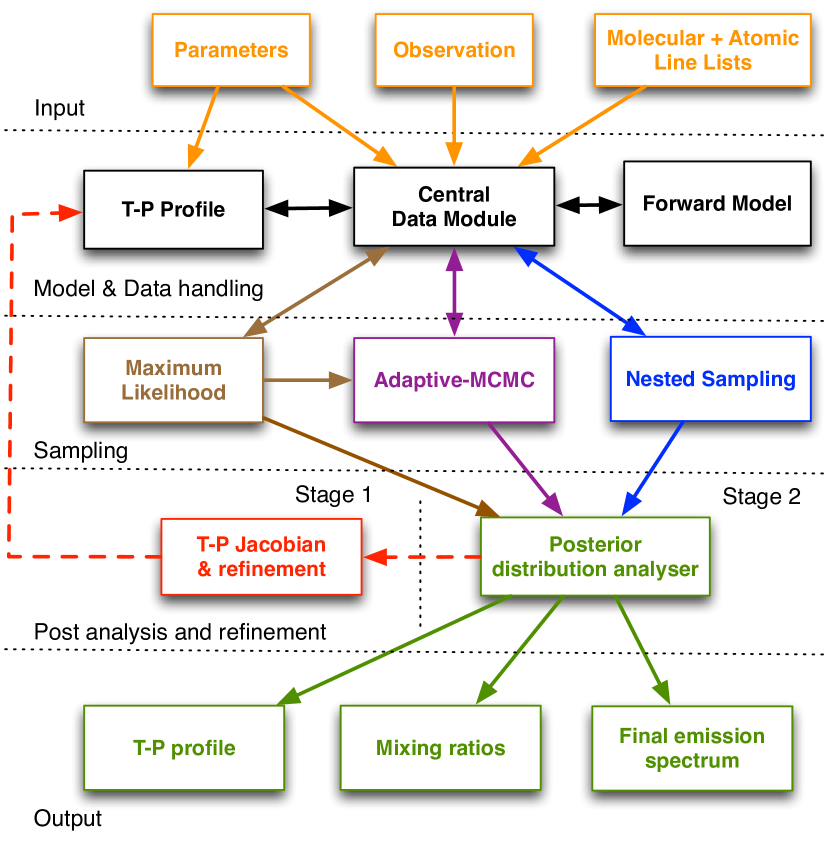
Figure 1 shows a schematic diagram of the $\mathcal{T}$-REx architecture for the emission retrieval. The program can be subdivided into five sections:

1. Inputs: Program inputs such as parameter files, molecular line-lists (ExoMol Tennyson & Yurchenko 2012), (HITEMP Rothman et al. 2010), stellar spectra (PHOENIX, Allard et al. 2012) and spectroscopic observations to be analysed.

2. Model & Data handling: The Central Data Module manages all calls to the TP-Profile and Forward Model Modules and provides a standardised, common interface to different sampling routines implemented.

3. Sampling: $\mathcal{T}$-REx features three independent sampling routines: Maximum Likelihood estimation (MLE, based on the LM-BFGS minimisation in W15), Markov Chain Monte Carlo (MCMC) and Nested Sampling (NS) routines. We refer the reader to W15 for implementation details.

4. Post analysis & refinement: This stage differs from W15 by providing a two iteration stages for the determination of the TP-Profile, see section 3.

5. Output: The final posterior distributions are analysed and the final model spectrum, TP-Profile and mixing ratios are returned.

Figure 1: Flowchart illustrating the modular design of $\mathcal{T}$-REx. This flowchart is an update from Waldmann et al. (2015), reflecting the differing architecture of the emission spectroscopy code.

2 Forward Model

We briefly describe the radiative transfer forward model, for a more exhaustive discussion we refer the reader to the standard literature (e.g., Chandrasekar 1960; Goody & Yung 1989; Liou 2002; Hanel et al. 2003; Mihalas & Mihalas 2013). In what follows, we closely follow the nomenclature of Liou (2002). For non-scattering atmospheres in local thermodynamic equilibrium, the basic equation describing the thermal radiation of an atmosphere is given by the Schwartzschild equation:

$$\mu\frac{dI_{\lambda}(\tau,\mu)}{d\tau}=I_{\lambda}(\tau,\mu)-B_{\lambda}(T)$$ (1)

where $I_{\lambda}$ is the intensity per wavelength, $\lambda$, $B_{\lambda}$ is the Planck function at temperature $T$, $\mu=\text{cos}\theta$ is the upwards inclination, $\tau$ is the overall optical depth, given as function of altitude ($z$) by

$${\tau}_{\lambda}(z)=\sum_{m=1}^{N_{m}}{\tau}_{\lambda,m}(z)$$ (2)

where $\tau_{\lambda,m}$ denotes the optical depth per absorbing species, $m$, given by

$$\tau_{\lambda,m}=\int_{z}^{z_{\infty}}{\varsigma}_{\lambda,m}(z^{\prime})\chi_{m}(z^{\prime})\rho_{N}(z^{\prime})\text{d}z^{\prime}.$$ (3)

Here ${\varsigma}_{\lambda,m}$ is the absorption cross section, $\chi_{m}$ the column density and $\rho_{N}$ the number density. We can now express the upwards welling radiance as

$$I_{\lambda}(\tau,\mu)=I_{\lambda}(\tau_{s})e^{-(\tau_{s}-\tau)/\mu}+\int_{\tau}^{\tau_{s}}B_{\lambda}(T_{\tau^{\prime}})e^{-(\tau^{\prime}-\tau)/\mu}\frac{\text{d}\tau^{\prime}}{\mu}$$ (4)

where the first right-hand-side term is the radiation at the planetary surface (or defined surface pressure for gaseous planets), and the second term denotes the integrated emission contributions for individual plane-parallel layers. The monochromatic transmittance and its derivative (weighting function) can be defined as

$$\mathcal{T}_{\lambda}(\tau)=e^{-\tau},\leavevmode\nobreak\ \leavevmode\nobreak\ \leavevmode\nobreak\ \leavevmode\nobreak\ \frac{\partial\mathcal{T}_{\lambda}(\tau)}{\partial\tau}=-e^{-\tau}.$$ (5)

Hence we express the total integrated radiation at the top of the atmosphere (TOA, $\tau=0,z=\infty$) as

$$I_{\lambda}(\tau=0)=B_{\lambda}(T_{s})e^{-\tau_{s}}+\int_{\tau_{s}}^{0}B_{\lambda}(T_{\tau})\frac{\partial\mathcal{T}_{\lambda}(\tau)}{\partial\tau}d\tau$$ (6)

where $\tau_{s}$ and $T_{s}$ are the optical depth and temperature at the planetary surface. The final exoplanetary emission spectrum is now given by

$$F_{P}/F_{\ast}=\frac{I_{\lambda}(\tau=0)}{I_{\ast}}\times\left(\frac{R_{P}}{R_{\ast}}\right)^{2}$$ (7)

here $I_{\ast}$ is the stellar intensity. By default $\mathcal{T}$-REx interpolates the stellar flux from a library of Phoenix stellar spectra, gridded at 100K intervals. Alternatively $\mathcal{T}$-REx can approximate the stellar intensity using a black-body at the stellar temperature.

3 Temperature - Pressure Profile

The determination of the vertical atmospheric temperature profile (also referred to as temperature-pressure profile or TP-profile for short) is one of the key challenges in the retrieval of atmospheric emission spectra. Typically two approaches exist in the retrieval of the TP-profile: 1) Layer-by-layer retrieval, 2) Analytic parameterisation.

1) The layer-by-layer approach consists of modelling the temperature of each plane-parallel atmospheric layer independently. This approach is usually adopted for retrieval work of the Earth’s atmosphere and solar system planets (Hanel et al. 2003; Rodgers 2000). The advantage of such an approach is its non-parametric nature, i.e. no prior knowledge is imposed on the temperature retrieval nor is the solution limited by potential restrictions and biases of an analytic TP-profile. The obvious disadvantage lies in the potentially poor convergence properties of such an approach in low S/N scenarios. Often, data quality or sparse spectral sampling do not allow for a pure layer-by-layer retrieval due to the large number of free parameters incurred. This is particularly true for current exoplanet spectroscopy data, which is either of relatively low S/N, low spectral resolution, or both. A common approach adopted is to impose a ‘regularisation’ of the TP-profile based on the physical reality that adjacent atmosphere layers should exhibit some correlation in temperature.

2) The second approach to the TP-profile retrieval is to adopt an analytic (here also referred to as ‘parametric’) model. Such models analytically approximate the mean underlying physics of the atmospheric thermal structure. Such models have the advantage of containing far fewer free parameters compared to the layer-by-layer approach, hence they converge faster. However, the solution is constrained within the bounds of the model assumed.

In summary, the layer-by-layer methodology is most objective but features poor convergence properties, whilst the parametric model is less objective but converges more robustly. For a review of existing implementations of both approaches in the field of exoplanet atmospheric retrieval we refer the reader to Line et al. (2013).

As described in section 3.2. $\mathcal{T}$-REx employs a hybrid model combining both, parametric and layer-by-layer approaches in a two stage retrieval process. In section 3.1 we briefly describe the parametric models implemented in $\mathcal{T}$-REx as part of the $\mathcal{T}$-REx retrieval framework.

3.1 Parametric Models in the literature

Analytical global-average TP-profiles exist in various flavours ranging from 2-stream purely radiative to radiative-convective approximations and global circulation models (GCMs). We refer the reader to the relevant literature for a more in-depth discussion on the various analytic approaches (e.g. Liou 2002; Hubeny et al. 2003; Hansen 2008; Burrows et al. 2008; Showman et al. 2009; Madhusudhan & Seager 2009; Pierrehumbert 2010; Guillot 2010; Heng et al. 2012, 2014; Robinson & Catling 2012). For the Stage 1 approach, $\mathcal{T}$-REx features a purely radiative 2-stream model as well as a choice of simpler TP-profiles based on purely geometric considerations (see 3.1.1). As described in section 3.2, the exact form of the TP-profile is less relevant in our case as the results will be refined in a second stage fitting.

Following Guillot (2010), the mean global temperature profile for a simple radiative downstream-upstream approximation can be expressed as

$$T^{4}(\tau)=\frac{3T^{4}_{int}}{4}\left(\frac{2}{3}+\tau\right)+\frac{3T^{4}_{irr}}{4}\xi_{\gamma_{1}}(\tau)$$ (8)

where $T_{int}$ is the planet internal heat flux, $T_{irr}$ the solar flux at the top of the atmosphere and

$$\xi_{\gamma_{i}}= \frac{2}{3}+\frac{2}{3\gamma_{i}}\left[1+\left(\frac{\gamma_{i}\tau}{2}-1\right)e^{-\gamma_{i}\tau}\right]$$ (9)

$$+\frac{2\gamma_{i}}{3}\left(1-\frac{\tau^{2}}{2}\right)E_{2}(\gamma_{i}\tau)$$

where $\gamma_{1}=\kappa_{\nu}/\kappa_{IR}$ is the ratio of mean opacities in the optical ($\kappa_{\nu}$) and infra-red ($\kappa_{IR}$) and $E_{2}$ is the second-order exponential integral given by

$$E_{n+1}(z)=\frac{1}{n}[e^{-z}-zE_{n}(z)].$$ (10)

We note that similar parameterisations exist in the literature (e.g., eq. (18), Robinson & Catling 2012; Pierrehumbert 2010). We also include the variation by Line et al. (2012) and Parmentier & Guillot (2014) including two optical opacity sources $\kappa_{\nu_{1}}$ and $\kappa_{\nu_{2}}$ and a weighting factor between optical opacities (left as free parameter) $\alpha$,

$$T^{4}(\tau)= \frac{3T^{4}_{int}}{4}\left(\frac{2}{3}+\tau\right)+\frac{3T^{4}_{irr}}{4}(1-\alpha)\xi_{\gamma_{1}}(\tau)$$ (11)

$$+\frac{3T^{4}_{irr}}{4}\alpha\xi_{\gamma_{2}}(\tau).$$

The temperature as function of opacity $\tau$ can be mapped to a pressure grid by assuming the following relation

$$\tau=\frac{\kappa_{IR}P}{g}.$$ (12)

3.1.1 Other TP-profiles

In addition to the above TP-profiles, we include an isothermal profile as well as a ‘3-point’ and ‘4-point’ profile. The 3-point profile is purely geometric and keeps the top of atmosphere temperature, $T_{TOA}$, the tropopause temperature and pressure, $T_{1}$, $P_{1}$, and the surface (or 10 bar pressure) temperature $T_{10bar}$ as free variables. The TP-profile is then linearly interpolated in ln$(P)$. The 4-point profile adds an extra variable temperature-pressure point to the profile.

3.2 The $\mathcal{T}$-REx Hybrid Model

Figure 2: Left: A given Temperature - Pressure Profile without inversion. Right: Correlation matrix $\mathcal{C}$, equation 14, of the TP-profile on the left. Atmospheric layers with similar temperatures feature a high layer-layer correlation whilst layers with temperature differences feature a lower correlation.

In $\mathcal{T}$-REx we have worked towards a hybrid solution of the above mentioned approaches in which the final solution is not bound by a parametric model but does not inherit the potentially poor convergence properties (and susceptibility to noise) of a layer-by-layer approach. Here we proceed in two stages: 1) We perform a parametric model retrieval, 2) we take the retrieval solution to ‘guide’ a second layer-by-layer retrieval, relaxing the parametric model constraint and thereby fine-tuning the TP-profile.

3.2.1 Stage 1

In Stage 1 we adopt a classical parametric model retrieval using one of the TP-profile parameterisations implemented in $\mathcal{T}$-REx. The idea is to constrain an initial best-fit of the model and whilst a realistic model (i.e. one well suited to describe the underlying TP-profile) is preferable, it is not a hard requirement. We now fit the solution using either of $\mathcal{T}$-REx’s sampling routines (MLE, MCMC, NS). The error on the sampled parametric model parameters is converted to one $\sigma$ lower and upper temperature bounds for a layer-by-layer model. This is done using a numerical model permutation analysis of the Stage 1 parameters.

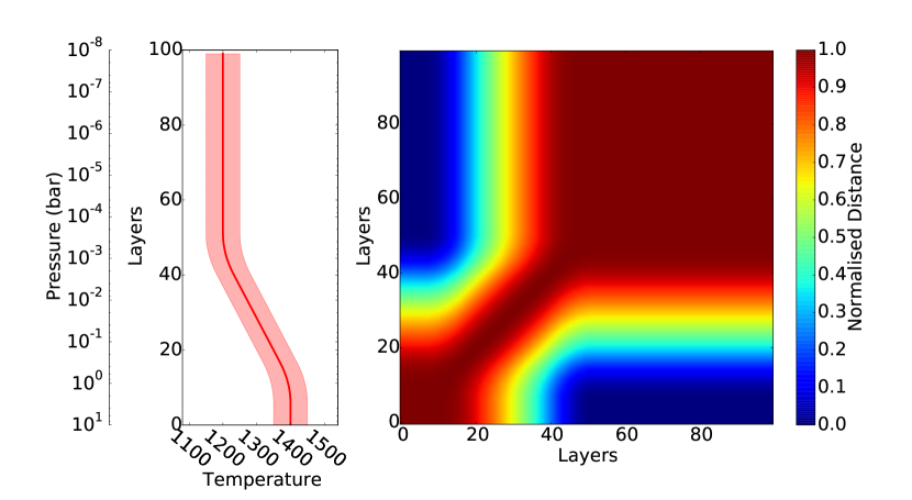
We then calculate the following distance matrix

$$\Delta^{2}_{ij}=|\hat{T}_{i}-\hat{T}_{j}|^{2}+(\sigma_{i}+\sigma_{j})^{2}$$ (13)

where $\hat{T}$ is the maximum likelihood temperature estimator of the parametric model fit for the $i^{th}$ and $j^{th}$ atmospheric layer and $\sigma$ is the respective error. Equation 13 captures the layer to layer temperature variations in the TP-profile and is hence conceptually similar to the Jacobian of the profile. We normalise $\Delta_{ij}$ in terms of the minimal and maximal temperature variations found in the TP-profile,

$$\mathcal{C}_{ij}=1.0-\frac{\Delta_{ij}-\text{argmin}\leavevmode\nobreak\ \Delta}{\text{argmax}\leavevmode\nobreak\ \Delta}$$ (14)

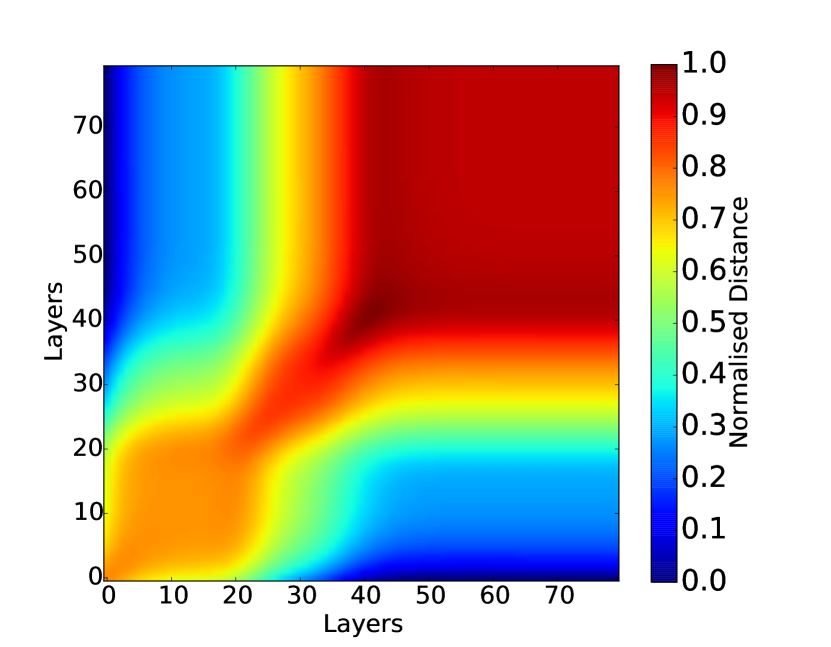
which can be understood as a positively defined temperature correlation matrix with layers most similar in temperature featuring the highest correlation and layers most dissimilar resulting in a very low correlation. An example of $\mathcal{C}$ for a given TP-profile can be found in fig. 2.

3.2.2 Stage 2

In the second stage of our TP-profile retrieval we relax the original solution found in Stage 1 and by that ‘fine-tune’ the TP-profile. We construct a second correlation matrix imposing an exponential correlation length across pressure levels (Rodgers 1976, 2000)

$$S_{ij}=(S_{ii}S_{jj})^{1/2}\text{exp}\left(-\frac{|ln(P_{i}/P_{j})|}{c}\right)$$ (15)

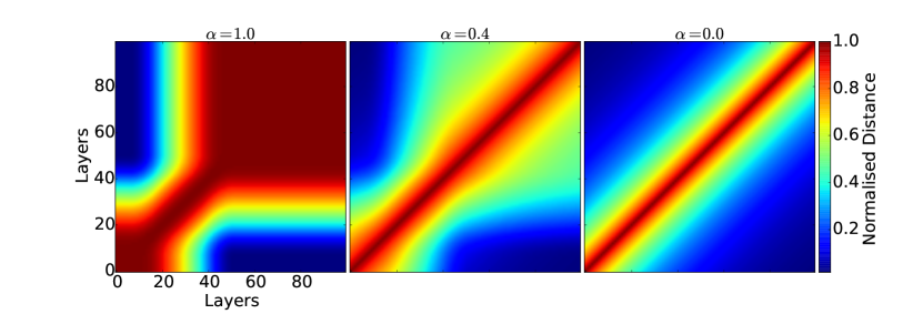
where $c$ is the correlation length in terms of atmospheric scale heights. We set $c=3.0$ by default, but can otherwise be user defined. Rodgers (2000) gives an advisable range between 1.0 - 8.0, with Irwin et al. (2008) using a default of $c=1.5$ and Line et al. (2013) $c=7.0$. Larger values of $c$ correspond to a stronger regularisation of the TP-profile (i.e. smoothing). A stronger regularisation can be useful in poorly constrained data sets (either low S/N, sparsely sampled or both). Equation 15 is identical to that used in the layer-by-layer approach by Irwin et al. (2008). We now construct a hybrid correlation matrix by combining equations 14 & 15

$$\mathcal{D}_{ij}(\alpha)=\alpha\mathcal{C}_{ij}+(1-\alpha)S_{ij}$$ (16)

where $\alpha$ is a scaling factor ranging from zero to one. Figure 3 shows instances of $\mathcal{D}(\alpha)$ at varying values of $\alpha$. We now correlate our layer-by-layer TP-profile with $\mathcal{D}(\alpha)$ whereby leaving $\alpha$ as free parameter to be fitted. By allowing $\alpha$ to vary, we can dynamically relax the parametric model solution from Stage 1, $\alpha=1.0$, to an unconstrained solution, $\alpha=0.0$. The advantage of such an approach is twofold: 1) Since the Stage 1 fitting should have already achieved a solution close to the real maximum likelihood, convergence in the second stage towards the volume of lowest $\chi^{2}$ is significantly faster; 2) $\mathcal{T}$-REx can freely decide to relax the Stage 1 solution should this be favoured by the data. Practically this happens frequently at later stages of the fitting. Whereas $\mathcal{T}$-REx initially converges towards the Stage 1 solution (i.e. $\alpha\rightarrow 1$), at later stages of the fitting the code begins to reject the parametric model (i.e. $\alpha\rightarrow 0$) as it ‘fine-tunes’ the original solution. This ‘tuning’ can achieve significantly higher maximum likelihoods than the Stage 1 fitting alone.

Figure 3: Hybrid correlation matrix $\mathcal{D}$, equation 16, at different values of $\alpha$. The left most is the pure Stage 1 correlation matrix, $\mathcal{C}$, whereas the right plot is the pure correlation-length-only matrix $S$, eq. (15). Over-plotted are contours of $\mathcal{D}(\alpha)$. The middle panel shows an intermediate state of left (60$\%$) and right (40$\%$).

3.3 Non-linear Sampling

Figure 4: Nonlinear TP-profile sampling on correlation matrix $\mathcal{C}$ (same as right hand plot in figure 2). Starting at the top of the atmosphere (red dot) we retain all layers in the TP-profile that correspond to a change in gradient $>2\%$ with respect to the previously retained layer until the bottom layer (green dot) is reached. The selected layers are denoted by white dots and arrows represent the path of the compression algorithm across the correlation matrix $\mathcal{C}$. Should no gradient change be detected for $>10$ layers, an extra sampling point is introduced (black dots).

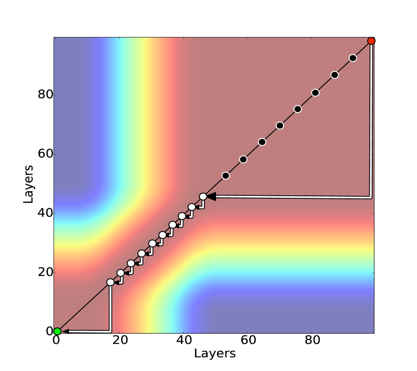
In the approach explained in section 3.2, we keep an even sampling of atmospheric layers in log($P$) for Stage 2. For well sampled and high S/N data, this approach is adequate. However for coarsely sampled and/or poor S/N data, it is often advisable to reduce the number of free parameters to a minimum to aid convergence. In these cases we can utilise the sparsity of the Stage 1 TP-profile solution to devise a nonlinearly sampling of the exoplanetary atmosphere. We base our compression algorithm on the fact that only changes in the temperature-pressure gradient need to be modelled, i.e., an isothermal TP-profile can be perfectly described by a single temperature parameter whereas areas of non-isothermal structure need more parameters to capture variation. The compression algorithm uses the Stage 1 correlation matrix $\mathcal{C}$ to only retain TP-profile layers corresponding to a $>2\%$ change in the TP gradient with respect to the previously retained layer. We graphically depict this in figure 4. In addition to TP-profile layers sampled this way, we also include an extra sampling layer whenever no change in thermal gradient was detected for $>10$ layers. The majority of the TP-profile variations should be captured by the Stage 1 retrieval and Stage 2 is ‘fine-tuning’ this solution. The inclusion of a coarse sampling in isothermal regimes does allows the Stage 2 retrieval to deviate from any Stage 1 solution, should this be supported by a higher global likelihood. Using the non-linear sampling, we can reduce a 100 layer atmospheric model to typically 15-25 free parameters.

4 Validation of $\mathcal{T}$-REx

We demonstrate the emission spectroscopy retrieval with two simulations and the secondary eclipse spectrum of HD189733b. The simulations are as follows: 1) high S/N observation simulation of a hot Jupiter similar to WASP-76b; 2) observations of the hot SuperEarth 55 Cnc e, simulated for a 1 meter class spectroscopic space mission. In our simulations we opt for two oxidised atmospheres at high temperatures ($>1500$K).

For each retrieval stage we calculate the global Bayesian Evidence of the solution set. Here the Bayesian Evidence (E, or simply Evidence hereafter) is given as the integral of the product of the global likelihood and the prior space

$$E=\int P({\bm{\theta}}|\mathcal{M})P({\bf x}|{\bm{\theta}},\mathcal{M})\text{d}{\bm{\theta}}$$ (17)

where $P({\bm{\theta}}|\mathcal{M})$ is the prior over the parameter space ${\bm{\theta}}$, for retrieval model $\mathcal{M}$. $P({\bf x}|{\bm{\theta}})$ is the likelihood for the observed data vector ${\bf x}$ given the parameter space and retrieval model. Retrieval Evidences are reported in tables 1 and 2.

4.1 WASP-76b

Figure 5: Correlation matrix, $\mathcal{C}$, derived from Stage 1 TP-profile shown in figure 7. The input model TP-profile is shown as black continuous line. Otherwise identical to figure 3.

Figure 6: showing the input spectrum of a WASP-76b type hot-Jupiter, gray, and Stage 1 & 2 fitting on the top and bottom respectively. Both fits converged but the Stage 2 fit reached a higher maximum likelihood.

Figure 7: TP-profiles for Stage 1 & 2 results for WASP-76b in figure 6. Solid lines represent the mean and shaded regions the one sigma error bars. Solid black lines are the input TP-profile. Stage 2 takes the initial parametric TP-profile fit of Stage 1 and relaxes the solution. Four solutions were obtained for Stage 1, the highest maximum likelihood solution (blue) traces the input TP-profile well, whilst local maxima underestimate the bulk temperature, see text. The Stage 2 solution feature a significantly lower $\chi^{2}$ (or higher global Evidence) than all Stage 1 solutions.

Figure 8: Left, retrieved TP-profile, right: contribution functions for WASP-76b. First and second row: Best-fit TP-profiles and corresponding emission contribution functions as function of pressure and wavelength for Stage 1 and Stage 2 respectively. Bottom row: Difference between both stages. Contribution difference is given as normalised fraction.

Table 1: Retrieved abundances for hot Jupiter WASP-76b. Top row: log Bayesian Evidence for Stage 1 & Stage 2 models. Differences above $|\Delta\text{log}(E)=5|$ are very significant. Here $\Delta\text{log}(E)=+80.12$ indicating a significantly improved fit in Stage 2.

	Input Model	Stage 1 Retrieval	Stage 2 Retrieval
log($E$)	NA	-43.92	36.20
log(H2O)	-4.0	-3.458 $\pm$ 0.104	-3.660 $\pm$ 0.107
log(CO)	-4.69	-4.352 $\pm$ 0.143	-4.548 $\pm$ 0.113
log(CO2)	-6.0	-5.374 $\pm$ 0.120	-5.428 $\pm$ 0.114

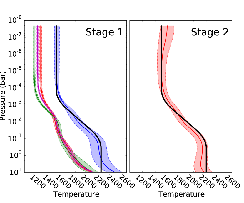
WASP-76b (West et al. 2013) is a very hot-Jupiter orbiting a late F7 star. It is highly inflated at $1.83^{+0.06}_{-0.04}$ $R_{Jup}$, $0.92\pm 0.03$ $M_{Jup}$ and $T_{equ}\sim 2200$K. We take its bulk and orbital properties and generate a simulated observation at a resolution of 300, spectral range of 0.5 - 20$\mu$m and 100ppm errors. We set the atmospheric composition to $1\times 10^{-4}$ H₂O, $1\times 10^{-5}$ CO and $1\times 10^{-5}$ CO₂. The input TP-profile is shown in figure 7 (black line). It is important to note that here (as well as in section 4.2) the input TP-profile was generated using a script external to $\mathcal{T}$-REx with no relation to either Stage 1 parametrisation. This provides an adequate test-bed for the Stage 1 fitting to accurately retrieve an arbitrary atmospheric profile.

As described in section 3.2, we retrieve the TP-profile and abundances in two stages. For computational efficiency reasons, here we only compute the Nested Sampling solutions (which are also the most accurate, see W15). Tests were run with both maximum-likelihood retrievals and MCMC retrievals and solutions between all sets of solutions are in good agreement.

The Nested Sampling Stage 1 solution returns four local likelihood maxima of which the global maximum was selected. Figures 6 (top), 7 (left) and table 1 show the retrieved spectrum, TP-profile and retrieved abundances respectively. The Stage 1 TP-profile mostly captures the input TP-profile but shows unrealistic bumps and wiggles as well as unrealistic distributions of the one sigma error bar. These are artefacts of the parameterisation in section 3.1. The three local maxima TP-profiles shown in figure 7 underestimate the bulk temperature of the planet, driving the retrieval to assume unrealistically low abundances of molecular trace gases. In this example this is found to be a numerical effect that disappears by increasing the sampling grid density of the Nested Sampling. Nonetheless the potential degeneracy between TP-profile and molecular abundances is in atmospheric retrievals is worth noting.

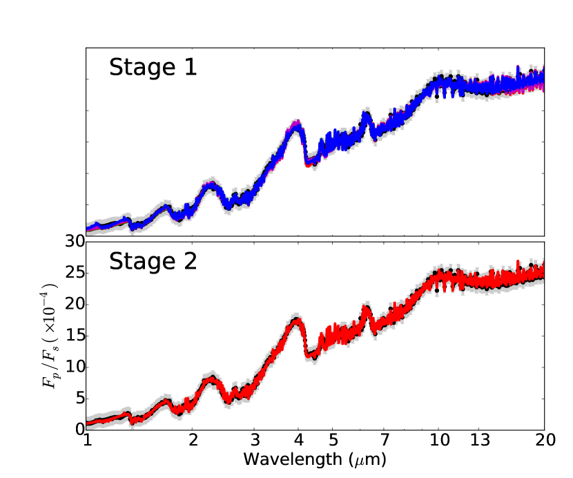
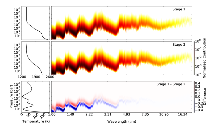
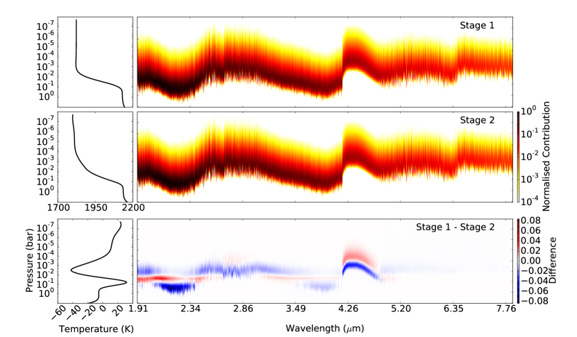
As described earlier, we computed the TP-profile covariance, $\mathcal{C}$ (figure 5), and tuned the Stage 1 retrieval by relaxing the parametric solution. Figures 6 (bottom), 7 (right) and table 1 show the Stage 2 retrieval results. Inspecting figure 6, both Stage 1 and Stage 2 retrievals fit the input spectrum sufficiently well but Stage 2 comes significantly closer to the ‘true’ TP-profile and trace gas abundances. Figure 8 shows the normalised emission contribution functions of both retrievals and their difference. This shows the planetary emission mainly emanating in the non-isothermal regions (up to the tropopause) of the TP-profile, as expected. However Stage 2 emissions originate significantly lower (by nearly an order of magnitude) in the atmosphere (blue band in the bottom panel).

4.2 55 Cnc e

Figure 9: Input spectrum of a 55 Cnc e type atmosphere, gray, and Stage 1 & 2 fitting on the top and bottom respectively. Both fits converged but the Stage 2 fit reached a higher global Evidence.

Figure 10: TP-profiles for Stage 1 & 2 results for 55 Cnc e in figure 9. Both solutions converge within the calculated error bar. Stage 2 features a significant improvement in maximum likelihood achieved.

Figure 11: Correlation matrix, $\mathcal{C}$, derived from Stage 1 TP-profile shown in figure 10. Otherwise identical to figure 5.

Figure 12: showing the model fit difference between Stage 1 and Stage 2 at spectral resolution of 1000. Model fit difference are of the order of $2\times 10^{-5}$ or less.

Figure 13: Contribution functions for 55Cnc e, otherwise same as figure 8.

Table 2: Retrieved abundances for hot SuperEarth 55 Cnc e. Top row: log Bayesian Evidence for Stage 1 & Stage 2 models.

	Input Model	Stage 1 Retrieval	Stage 2 Retrieval
log($E$)	NA	75.40	168.90
log(H2O)	-4.0	-4.168 $\pm$ 0.795	-4.055 $\pm$ 0.571
log(CO)	-5.0	-5.764 $\pm$ 1.248	-5.613 $\pm$ 1.172
log(CO2)	-5.0	-5.236 $\pm$ 1.112	-5.136 $\pm$ 1.019

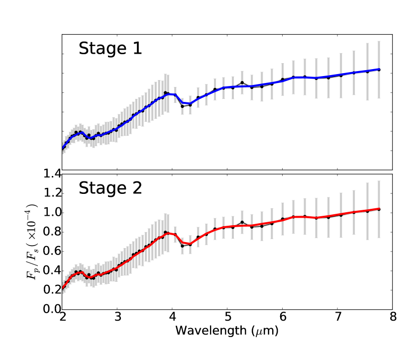
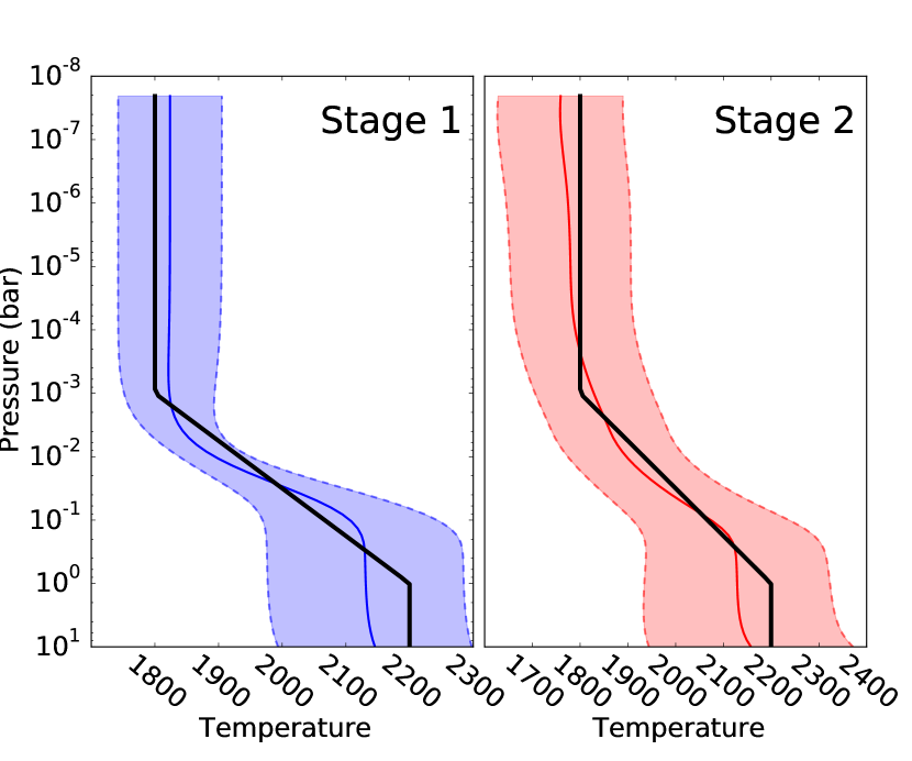
We simulated an emission spectrum of the hot SuperEarth 55 Cnc e (Fischer et al. 2008). We use trace gas compositions of $1\times 10^{-4}$ H₂O, $1\times 10^{-5}$ CO and $1\times 10^{-5}$ CO₂ and a sharp TP-profile shown in fig.10. As the previous WASP-76 example is currently unrealistically optimistic, given the combination of high S/N, moderate resolution (R$\sim$ 300) and a very broad wavelength coverage, we opt for a more realistic example here. We calculated the expected resolution and S/N for 100 co-added eclipses obtained by a one-meter-class transiting spectroscopy space-mission (e.g. the ESA M4 proposal ARIEL) over a wavelength range spanning 2 to 8$\mu$m. Using EChOSim, an end-to-end simulator for transit spectroscopy space-missions (Pascale et al. 2014; Waldmann & Pascale 2014) developed for the ESA M3 EChO proposal (Tinetti et al. 2012), we calculated realistic error bars for this hot SuperEarth, shown in figure 9.

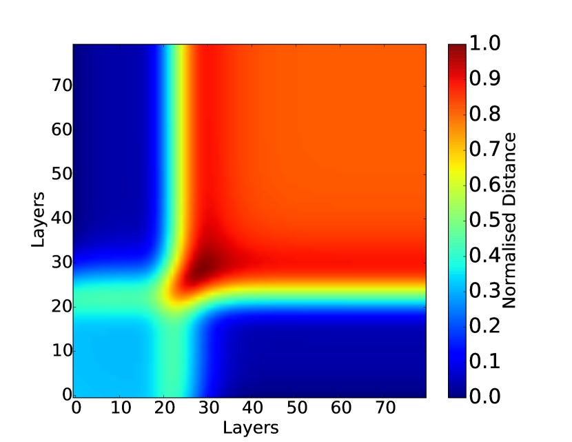
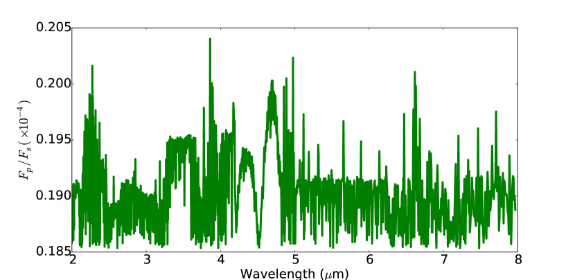
Similarly to section 4.1, figs 9, 10 & 11 show the Stage 1 & 2 retrieved spectra, TP-profiles and Stage 1 TP-profile covariance respectively. Table 2 shows that Stage 2 retrieval converges at a significantly higher global Evidence and presents an improvement in the accuracy of abundances retrieved as well as TP-profile retrieved. Figure 12 shows the absolute difference between the Stage 1 and Stage 2 model fits at a spectral resolution of 1000. Here the discrepancies between both spectral fits are of the order of $2\times 10^{-5}$ or less. This is not very significant in terms of a naive $\chi^{2}$ fit to relatively low S/N data, but does significantly drive the retrieval of the TP-profile and trace gas abundances. This is reflected in the Bayesian Evidence measured for Stage 1 and Stage 2 models. Figure 13 shows the contribution functions for both retrievals. Here we have positive and negative temperature differences (see bottom left plot), resulting in a more complex contribution differential (bottom left plot) than for WASP-76b. It should be noted that this contribution differential is highly wavelength dependent and illustrates the sensitivity of varying wavelength ranges on the TP-profile retrievability.

4.3 HD189733b

Figure 14: Emission spectrum of a HD189733b, black circles, and Stage 1 & 2 fitting on the top and bottom respectively; blue: the fitted emission spectrum at R=1000; red squares: spectrum fit binned to data resolution; grey: photometric passbands for Spitzer/IRAC and MIPS. Both fits converged but the Stage 2 fit reached a higher global Evidence.

Figure 15: TP-profiles for Stage 1 & 2 results for HD189733b in figure 14. Both solutions converge within the calculated error bar. Stage 2 features a significant improvement in maximum likelihood achieved.

Figure 16: Correlation matrix, $\mathcal{C}$, derived from Stage 1 TP-profile shown in figure 15. Most of the atmosphere is found to be best fit with an isothermal profile but the lowest $\sim$ 20 atmospheric layers ($\sim$ 0.1 bar). Otherwise identical to figure 5.

Figure 17: Marginalised and conditional posterior distributions of the trace gasses of HD189733b for Stage 1 fitting. All trace gases are well constrained but only an upper limit to methane can be found.

Figure 18: Marginalised and conditional posterior distributions of the trace gasses of HD189733b for Stage 2 fitting. All trace gases are well constrained.

Figure 19: Model fit difference between Stage 1 and Stage 2 at spectral resolution of 1000. Differences between either retrievals are of the order of 5-8$\times 10^{-4}$ in most wavelengths.

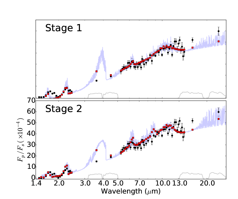
Finally we test $\mathcal{T}$-REx on the emission spectrum of the hot Jupiter HD189733b. Its emission spectrum is amongst the most complete and best studied (e.g. Swain et al. 2009; Madhusudhan & Seager 2009; Lee et al. 2011; Line et al. 2012, 2014). We have compiled data sets ranging from the NIR (1.4$\mu$m) to the MIR (24$\mu$m), namely: HST/NICMOS (Swain et al. 2009), Spitzer/IRAC 3.6, 4.5 $\mu$m (Knutson et al. 2012), 8.0 $\mu$m (Agol et al. 2010), Spitzer/IRS spectroscopy (Grillmair et al. 2008), Spitzer/IRS 16 & 24 $\mu$m photometry (Charbonneau et al. 2008). As in previous studies, we consider the active trace gasses H₂O, CH₄, CO and CO₂ and otherwise assume a hydrogen dominated atmosphere.

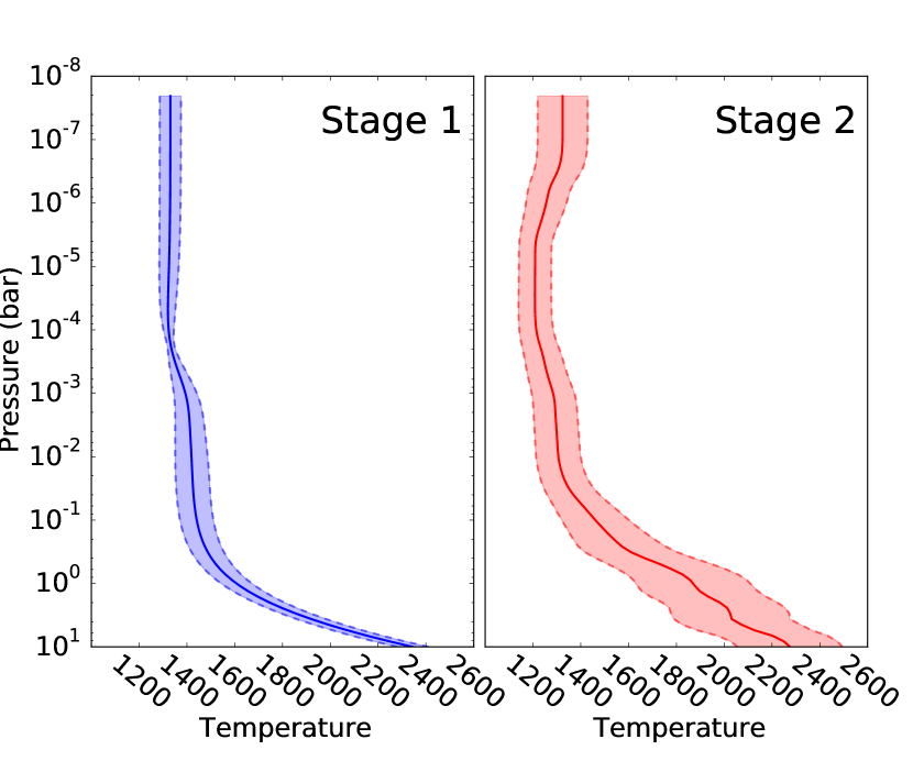
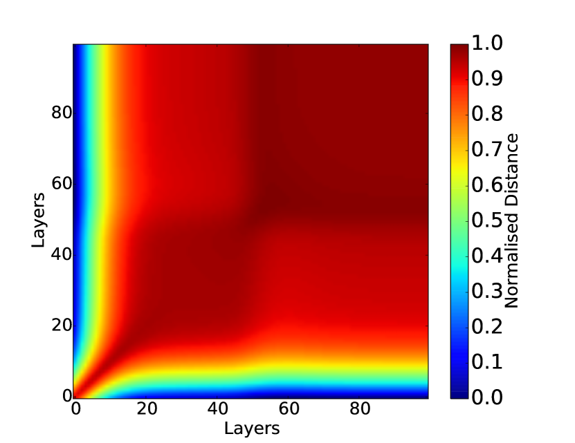
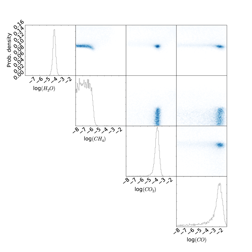
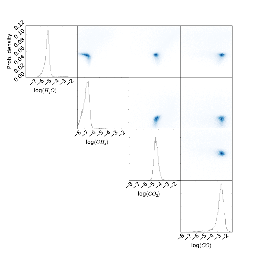
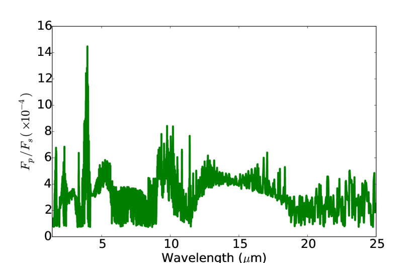
Figure 14 shows the retrieved emission models with retrieved abundances and log(Evidence) reported in table 3. Figures 15 and 16 report the retrieved Stage 1 & Stage 2 TP-profiles and associated Stage 1 TP-covariance, respectively. Figures 17 & 18 are the marginalised and conditional posteriors for the active trace gasses considered. Figure 19 illustrates the difference between Stage 1 and Stage 2 emission spectra.

As described above, the Stage 1 retrieval was first performed using the parmetric TP-profile by Guillot (2010) with the additional optical opacity terms proposed by Line et al. (2012). Here, all parameters of the TP model were allowed to vary. We modelled the atmosphere over 25 scale heights sampled onto a 150 pressure-layer grid. Following this initial retrieval the TP-covariance was computed resulting in a predominantly isothermal atmosphere down to the lowest $\sim$20 layers ($\sim$ 0.1 bar pressure). The obtained TP-profile is well constrained but shows systematics (e.g. at $5\times 10^{-4}$ bar) typical to this type of parametrisation. The posterior distributions of the active trace gases, figure 17 shows good constrains on abundances. From figure 17, we can see the retrieved values for methane to only constitute an upper limit.

The Stage 2 hybrid model contained 22 free parameters on its non-linearly sampled TP-profile grid. All parameters were allowed to vary freely between fully constrained ($\alpha=1.0$ in equation 16) and unconstrained scenarios. Figure 15 (right) shows the Stage 2 TP-profile with $\alpha=0.54$, indicating a significant shift away from the parametric solution of ${\it Stage\leavevmode\nobreak\ 1}$. The Stage 2 model features a lower tropopause pressure along with reduced water and carbon-dioxide abundances to achieve a very significant increase in Bayesian Evidence, see table 3 and discussion in section 5. The Stage 2 TP-profile error bounds are slightly larger. Given a significantly higher Evidence for Stage 2, it is indicative of Stage 1 TP-profile errors to be underestimated by the parameterisation used. The posteriors distributions of Stage 2 now show a convergence of methane beyond the upper-bound constrained of Stage 1.

Compared to table 3 in Line et al. (2014), we obtain lower abundances of CH₄ and CO₂ but higher values for CO. Whereas these values differ from previous analyses, we find them significantly closer to the chemical model predictions of HD189733b (e.g. Line et al. 2010; Venot et al. 2012; Moses et al. 2013). Note that also Stage 1 results exhibit the same trend of lower CH₄ and CO₂ abundances. We find two aspects by which our analysis differs from others in the literature: 1) A finer and complete sampling of correlated likelihoods, in particular compared to maximum likelihood methods which are often less efficient with sparsely sampled data; 2) The completeness of molecular line-lists used. This is particularly true for the C/O ratio determination using CH₄ and CO/CO₂ as tracers. In this work we use the new YT10to10 CH₄ line-list (Yurchenko & Tennyson 2014).

Table 3: Retrieved abundances for hot Jupiter HD189733b. Top row: log Bayesian Evidence for Stage 1 & Stage 2 models. $\Delta\text{log}(E)=+121.75$ indicating a very significant improvement in the Stage 2 fit compared to Stage 1.

	Stage 1 Retrieval	Stage 2 Retrieval
log($E$)	-43.23	78.52
log(H2O)	-3.918 $\pm$ 0.207	-4.978 $\pm$ 0.602
log(CH4)	-6.732 $\pm$ 0.719	-6.768 $\pm$ 0.487
log(CO2)	-3.722 $\pm$ 0.482	-4.204 $\pm$ 0.488
log(CO)	-2.671 $\pm$ 1.387	-2.689 $\pm$ 0.769

5 Discussion

In section 4 we have demonstrated the efficiency of the $\mathcal{T}$-REx retrieval suite for emission spectroscopy using a simulated hot-Jupiter, a hot-SuperEarth, as well as secondary eclipse observations of HD189733b, as examples.

In all three cases the Bayesian Evidence of the Stage 2 retrieval is significantly higher, log($E$) = 36.20 compared to - 43.92, log($E$) = 168.9 to 75.40, log($E$) = -43.23 to 78.52 for WASP-76b, 55 Cnc e and HD189733b, respectively. This is clearly indicative of Stage 2 results being more robust statistically. Following the adaptation of the Jeffrey’s scale of model evidence (Jeffreys & Kendall 1948) by Kass & Raftery (2012), we can define a strong preference for the Stage 2 model as $\Delta\text{log}(E)>5$ and equally, a strong preference of the Stage 1 model to be $\Delta\text{log}(E)<-5$. Evidence differences ranging from -5 to 5 indicate a lesser significance. In the case of WASP-76b we find $\Delta\text{log}(E)=+80.12$, $\Delta\text{log}(E)=+132.70$ for 55 Cnc e and $\Delta\text{log}(E)=+121.75$ for HD189733b. Furthermore the improved Stage 2 fit is illustrated by the better retrieval of the trace gas abundances (tables 1, 2 & 3). This illustrates the importance of accurate TP-profile retrievals and the advantage of a two-staged approach, especially in cases of low resolution and/or low S/N data.

6 Conclusion

In this paper we introduced the emission spectroscopy retrieval approach for the $\mathcal{T}$-REx retrieval suite framework. Given a common code basis for transmission and emission retrieval, allows us to benefit from computational efficiencies and the high accuracy of molecular line-list handling introduced in W15. To suite the needs of the temperature-pressure profile retrieval, we implemented an extra loop unique to the emission side of $\mathcal{T}$-REx, which allows a two-staged retrieval. We show that such a staged retrieval of the emission spectrum (and TP-profile) allows us to dynamically scale the complexity of the retrieval problem (from a fully parameterised to a fully unconstrained model) and has significant advantages in accuracy and robustness over previously available methods. Future publications will extend the sensitivity analyses presented here to include present and future ground and space instrumentation and a wider range of planets observable in emission spectroscopy.

References

- Agol et al. (2010) Agol, E., Cowan, N. B., Knutson, H. A., et al. 2010, ApJ, 721, 1861
- Allard et al. (2012) Allard, F., Homeier, D., & Freytag, B. 2012, Philosophical Transactions of the Royal Society A: Mathematical, Physical and Engineering Sciences, 370, 2765
- Burrows et al. (2008) Burrows, A., Budaj, J., & Hubeny, I. 2008, The Astrophysical Journal, 678, 1436
- Chandrasekar (1960) Chandrasekar, H. 1960, Radiative Transfer (New York: Dover Publications)
- Charbonneau et al. (2008) Charbonneau, D., Knutson, H. A., Barman, T., et al. 2008, ApJ, 686, 1341
- Conrath et al. (1973) Conrath, B., Curran, R., Hanel, R., et al. 1973, Journal of Geophysical Research, 78, 4267
- Conrath et al. (1970) Conrath, B. J., Hanel, R. A., Kunde, V. G., & Prabhakara, C. 1970, Journal of Geophysical Research, 75, 5831
- Fischer et al. (2008) Fischer, D. A., Marcy, G. W., Butler, R. P., et al. 2008, APJ, 675, 790
- Fletcher et al. (2007) Fletcher, L. N., Irwin, P. G. J., Teanby, N. A., et al. 2007, ICARUS, 189, 457
- Goody & Yung (1989) Goody, R. M., & Yung, Y. L. 1989, Atmospheric Radiation (Oxford: Oxford University Press)
- Griffith (2014) Griffith, C. A. 2014, Philosophical Transactions of the Royal Society A: Mathematical, 372, 30086
- Grillmair et al. (2008) Grillmair, C. J., Burrows, A., Charbonneau, D., et al. 2008, Nature, 456, 767
- Guillot (2010) Guillot, T. 2010, Astronomy and Astrophysics, 520, A27
- Hanel et al. (1981) Hanel, R., Conrath, B., Flasar, F. M., et al. 1981, Science, 212, 192
- Hanel et al. (2003) Hanel, R. A., Conrath, B., J., Jennings, D. E., & Samuelson, R. E. 2003, Exploration of the Solar System by Infrared Remote Sensing (Cambridge: Cambridge University Press)
- Hanel et al. (1972) Hanel, R. A., Conrath, B. J., Hovis, W. A., et al. 1972, Science, 175, 305
- Hansen (2008) Hansen, B. M. S. 2008, The Astrophysical Journal Supplement Series, 179, 484
- Heng et al. (2012) Heng, K., Hayek, W., Pont, F., & Sing, D. K. 2012, Monthly Notices of the Royal Astronomical Society, 420, 20
- Heng et al. (2014) Heng, K., Mendonça, J. M., & Lee, J.-M. 2014, The Astrophysical Journal Supplement, 215, 4
- Hubeny et al. (2003) Hubeny, I., Burrows, A., & Sudarsky, D. 2003, ApJ, 594, 1011
- Irwin et al. (2008) Irwin, P. G. J., Teanby, N. A., De Kok, R., et al. 2008, Journal of Quantitative Spectroscopy & Radiative Transfer, 109, 1136
- Jeffreys & Kendall (1948) Jeffreys, H., & Kendall, M. G. 1948, The Mathematical Gazette, 32, 304
- Kaplan (1959) Kaplan, L. D. 1959, Journal of the Optical Society of America, 49, 1004
- Kass & Raftery (2012) Kass, R. E., & Raftery, A. E. 2012, Journal of the American Statistical Association, 90, 773
- King (1958) King, J. I. F. 1958, Scientific Uses of Earth Satellites: Second Revised Edition. Edited by James A. Van Allen. Published by the University of Michigan Press, -1, 133
- Knutson et al. (2012) Knutson, H. A., Lewis, N., Fortney, J. J., et al. 2012, ApJ, 754, 22
- Lee et al. (2011) Lee, J. M., Fletcher, L. N., & Irwin, P. G. J. 2011, Monthly Notices of the Royal Astronomical Society, 420, 170
- Line et al. (2014) Line, M. R., Knutson, H., Wolf, A. S., & Yung, Y. L. 2014, ApJ, 783, 70
- Line et al. (2010) Line, M. R., Liang, M. C., & Yung, Y. L. 2010, APJ, 717, 496
- Line et al. (2012) Line, M. R., Zhang, X., Vasisht, G., et al. 2012, The Astrophysical Journal, 749, 93
- Line et al. (2013) Line, M. R., Wolf, A. S., Zhang, X., et al. 2013, The Astrophysical Journal, 775, 137
- Liou (2002) Liou, K. N. 2002, An introduction to atmospheric radiation (London: Academic Press)
- Madhusudhan & Seager (2009) Madhusudhan, N., & Seager, S. 2009, The Astrophysical Journal, 707, 24
- Mihalas & Mihalas (2013) Mihalas, D., & Mihalas, B. W. 2013, Foundations of Radiation Hydrodynamics (Courier Corporation)
- Moses et al. (2013) Moses, J. I., Madhusudhan, N., Visscher, C., & Freedman, R. S. 2013, ApJ, 763, 25
- Parmentier & Guillot (2014) Parmentier, V., & Guillot, T. 2014, Astronomy and Astrophysics, 562, 133
- Pascale et al. (2014) Pascale, E., Waldmann, I. P., MacTavish, C. J., et al. 2014, arXiv.org, 1406.3984
- Pierrehumbert (2010) Pierrehumbert, R. T. 2010, Principles of Planetary Climate
- Robinson & Catling (2012) Robinson, T. D., & Catling, D. C. 2012, APJ, 757, 104
- Rodgers (1976) Rodgers, C. D. 1976, Reviews of Geophysics and Space Physics, 14, 609
- Rodgers (2000) —. 2000, Inverse Methods for Atmospheric Sounding, Theory and Practice (World Scientific Publishing Company Incorporated)
- Rothman et al. (2010) Rothman, L. S., Gordon, I. E., Barber, R. J., et al. 2010, Journal of Quantitative Spectroscopy & Radiative Transfer, 111, 2139
- Showman et al. (2009) Showman, A. P., Fortney, J. J., Lian, Y., et al. 2009, The Astrophysical Journal, 699, 564
- Swain et al. (2009) Swain, M. R., Vasisht, G., Tinetti, G., et al. 2009, The Astrophysical Journal Letters, 690, L114
- Tennyson & Yurchenko (2012) Tennyson, J., & Yurchenko, S. N. 2012, Monthly Notices of the Royal Astronomical Society, 425, 21
- Tinetti et al. (2013) Tinetti, G., Encrenaz, T., & Coustenis, A. 2013, The Astronomy and Astrophysics Review, 21, 63
- Tinetti et al. (2012) Tinetti, G., Beaulieu, J. P., Henning, T., et al. 2012, Experimental Astronomy, 34, 311
- Venot et al. (2012) Venot, O., Hébrard, E., Agúndez, M., et al. 2012, A&A, 546, A43
- Waldmann & Pascale (2014) Waldmann, I. P., & Pascale, E. 2014, Experimental Astronomy, arXiv:1402.4408
- Waldmann et al. (2015) Waldmann, I. P., Tinetti, G., Rocchetto, M., et al. 2015, The Astrophysical Journal, 802, 107
- Wark & Hilleary (1969) Wark, D. Q., & Hilleary, D. T. 1969, Science, 165, 1256
- West et al. (2013) West, R. G., Almenara, J. M., Anderson, D. R., et al. 2013, arXiv.org, 5607
- Yurchenko & Tennyson (2014) Yurchenko, S. N., & Tennyson, J. 2014, MNRAS, 440, 1649