Abstract

We give an analytic (free of computer assistance) proof of the existence of a classical Lorenz attractor for an open set of parameter values of the Lorenz model in the form of Yudovich-Morioka-Shimizu. The proof is based on detection of a homoclinic butterfly with a zero saddle value and rigorous verification of one of the Shilnikov criteria for the birth of the Lorenz attractor; we also supply a proof for this criterion. The results are applied in order to give an analytic proof of the existence of a robust, pseudohyperbolic strange attractor (the so-called discrete Lorenz attractor) for an open set of parameter values in a $4$-parameter family of three-dimensional Henon-like diffeomorphisms.

Keywords: Lorenz attractor, Henon map, homoclinic butterfly, separatrix value.

Mathematics Subject Classification: 34C37, 34C20, 37D45, 37C29.

1 Introduction

The main goal of the paper is a proof of the birth of the Lorenz attractor in the following model:

$$\begin{array}[]{l}\dot{X}=Y,\\ \dot{Y}=-\lambda Y+\gamma X(1-Z)-\delta X^{3}\\ \dot{Z}=-\alpha Z+\beta X^{2},\end{array}$$ (1)

where parameters $\alpha$, $\beta$, $\gamma$, $\delta$ and $\lambda$ can take arbitrary finite values. It is well-known [1, 2, 3] that the classical Lorenz equations

$$\begin{array}[]{l}\dot{x}=-\sigma(x-y),\\ \dot{y}=rx-y-xz\\ \dot{z}=-bz+xy\end{array}$$ (2)

can be always brought to form (1) by the transformation $\displaystyle x=X\sqrt{2},\;y=\sqrt{2}\left(\frac{Y}{\sigma}+X\right),\;z=(r-1)Z+\frac{X^{2}}{\sigma}$ with $\displaystyle\alpha=b,\;\;\beta=\frac{2\sigma-b}{\sigma(r-1)},\;\;\gamma=\sigma(r-1),\;\;\delta=1,\;\;\lambda=\sigma+1$. We therefore call system (1) the extended Lorenz model.

Not all values of parameters in system (1) correspond to real values of the parameters $(r,\sigma,b)$, so the proof of the Lorenz attractor in model (1) may not always imply the existence of the Lorenz attractor in the classical Lorenz model. In particular, the values of $\alpha$ and $\lambda$, for which the existence of the Lorenz attractor is proved in the present paper (see Theorem 1), do not correspond to the Lorenz model; instead, for these parameters values one can transform system (1) to the system obtained from the Lorenz model by the time reversal.

Nevertheless, system (1) is interesting by itself because it is a normal form for certain codimension-3 bifurcations of equilibria and periodic orbits [4, 5]. Thus, our result on the existence of the Lorenz attractor in system (1) automatically proves the emergence of the Lorenz attractor (or its discrete analogue) in a class of such bifurcations and, hence, in a large set of systems of various nature. In particular, in this paper, using Theorem 1 we prove the existence of discrete Lorenz attractors in a class of three-dimensional polynomial maps (3D Henon maps).

We consider the case $\gamma>0$, so by scaling the time and the coordinates we can make $\gamma=1$. When $\alpha\beta>0$, with the scaling $\beta=\alpha\delta/B$ one can bring system (1) to the form:

$$\begin{array}[]{l}\dot{X}=Y,\\ \dot{Y}=X-\lambda Y-XZ-BX^{3}\\ \dot{Z}=-\alpha(Z-X^{2}).\end{array}$$ (3)

In [4] it was shown numerically that system (3) possesses the Lorenz attractor in an open set of values of $(\alpha,\lambda)$ for each $B\in(-1/3,+\infty)$. In this paper we obtain an analytic proof of the same fact for sufficiently large $B$. The idea is that for $B=+\infty$ equations (3) can be solved explicitly. Therefore for large $B$ the system can be analysed using asymptotic expansions.

We perform such expansion for system (1) with $\gamma>0$, $\delta>0$. By coordinates and time scaling it can be brought to the form:

$$\begin{array}[]{l}\dot{X}=Y,\\ \dot{Y}=X-\lambda Y-XZ-X^{3}\\ \dot{Z}=-\alpha Z+\beta X^{2}.\end{array}$$ (4)

Obviously, large $B$ in system (3) corresponds to small $\beta$ in (4). The following theorem is our main result.

Theorem 1

For each sufficiently small $\beta$, in the $(\alpha,\lambda)$–plane there exists a point $\alpha=\alpha(\beta),\lambda=\lambda(\beta)$ for which system $($4$)$ possesses a double homoclinic loop $($a homoclinic butterfly$)$ to a saddle equilibrium with zero saddle value. This point belongs to the closure of a domain $V_{LA}(\beta)$ in the $(\alpha,\lambda)$–plane for which system $($4$)$ possesses an orientable Lorenz attractor.

In § 2 we give a definition of the Lorenz attractor, following [6]. This definition requires a fulfilment of a version of a cone condition at each point of a certain absorbing domain. We verify this condition by using one of the Shilnikov criteria [7, 8]. A partial case of these criteria was proven by Robinson [9, 10], however it was done under additional “smoothness of the foliation” assumption which is not fulfilled by system (4) at small $\beta$. Therefore we provide a full proof of the part of Shilnikov criteria relevant to our situation, see Theorem 2. In § 3 we prove Theorem 1.

In § 4 we prove (Theorem 3) the existence of discrete Lorenz attractors in a class of three-dimensional Henon maps. A discrete Lorenz attractor is a generalization of the strange attractor in the period map of a time-periodic perturbation of an autonomous flow with a Lorenz attractor [11, 12]. It is a pseudo-hyperbolic attractor in the sense of [13, 14]; like in the continuous-time Lorenz attractor, each orbit in the discrete Lorenz attractor has positive maximal Lyapunov exponent, and this property is robust with respect to small smooth perturbations of the map.

The discrete Lorenz attractors were found numerically in several 3D Henon maps [11, 12, 15] and in certain models of non-holonomic mechanics [16, 17]. The 3D Henon maps are particularly important because they serve as a zeroth order approximation to the rescaled first-return maps near various types of homoclinic and heteroclinic tangencies [18, 19, 20, 21, 22, 23]. Therefore, because of the robustness of the discrete Lorenz attractor, by showing that a 3D Henon map has such attractor we also show that the corresponding homoclinic or heteroclinic tangency bifurcation produces such attractor; moreover, when the corresponding tangency is persistent (e.g. due to the Newhouse mechanism [24, 25, 26, 27]) one obtains infinitely many coexisting discrete Lorenz attractors in a generic map from the corresponding Newhouse domain (see [22] for examples and more explanation). Obviously, in order to implement this construction completely rigorously, the numerical evidence is not enough, i.e. an analytic proof of the existence of the discrete Lorenz attractor in various classes of Henon maps is needed. Our Theorem 3 in § 4 is the first example of such proof.

We find that a certain codimension-4 bifurcation happens at certain parameter values to the fixed point of a 3D Henon map and show that the normal form for this bifurcation is given by the period map of a small time-periodic perturbation of system (4) at small $\beta$. Then, Theorem 1 implies Theorem 3 immediately. A less degenerate bifurcation (of codimension 3) that also occurs in the same class of maps produces, as a normal form, system (3) with $B=0$. This particular case is known as the Morioka-Shimizu system [28]. While a very detailed numerical analysis of the dynamics of this model is available [29, 30, 31, 32, 33] and the existence of the Lorenz attractor in the Morioka-Shimizu system causes no doubt, a rigorous analytic proof of this fact is lacking (see discussion in [34]). Its absence impedes the further development of the mathematical theory of the discrete Lorenz attractors. Obtaining such proof is a challenging and important problem; in particular, it would be interesting to know if a rigorous numerical proof of the existence of the Lorenz attractor in the Morioka-Shimizu system is possible, similar to that reported in [40, 41] for the classical Lorenz model.

2 Shilnikov criterion of the birth of Lorenz attractor

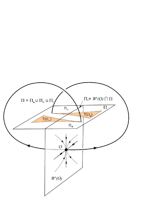
Figure 1: Afraimovich-Bykov-Shilnikov geometric Lorenz model.

Let us recall a definition of the Lorenz attractor. There are several approaches to it, which include classical geometric models by Guckenheimer-Williams [46, 47] and Afraimovich-Bykov-Shilnikov [35, 6] and their later generalisations [48, 49]. Here we define the Lorenz attractor in the Afraimovich-Bykov-Shilnikov sense.

Consider a smooth system of differential equations which has a saddle equilibrium state $O$ with one-dimensional unstable manifold. Take a cross-section $\Pi$ transverse to a piece of the stable manifold $W^{s}(O)$ (for system (4) the cross-section will be the plane $z=\beta/\alpha$). The one-dimensional manifold $W^{u}(O)$ consists of three orbits: $O$ itself, and two separatrices, $\Gamma_{+}$ and $\Gamma_{-}$. Let both $\Gamma_{+}$ and $\Gamma_{-}$ intersect the cross-section at some points $M_{+}$ and $M_{-}$. Let $\Pi_{0}$ be the first intersection of the cross-section with $W^{s}(O)$, and $\Pi_{+}$ and $\Pi_{-}$ be the regions on the opposite sides from $\Pi_{0}$, so $\Pi=\Pi_{+}\cup\Pi_{-}\cup\Pi_{0}$. Assume that in the cross-section there is a region $D\subset\Pi_{0}$ which is forward-invariant with respect to the Poincare map $T$ defined by the orbits of the system. When a point $M$ approaches $\Pi_{0}$ from the side of $\Pi_{+}$ we have $TM\to M_{+}$, and when it tends to $\Pi_{0}$ from the side of $\Pi_{-}$ we have $TM\to M_{-}$ (see Fig. 1). Thus, the invariance of $D$ implies that $M_{+}\in D$ and $M_{-}\in D$. Let us introduce coordinates $(u,v)$ in $\Pi$ such that $\Pi_{0}$ has equation $u=0$, $\Pi_{+}$ corresponds to $u>0$, and $\Pi_{-}$ corresponds to $u<0$. We write the map $T$ in the form

$$\bar{u}=f_{\pm}(u,v),\qquad\bar{v}=g_{\pm}(u,v),$$

where “$+$” corresponds to $u>0$ and “$-$” corresponds to $u<0$. The map is smooth at $u\neq 0$ but it becomes singular as $u\to 0$ because the return time to the cross-section tends to infinity as the starting point approaches the stable manifold of the equilibrium $O$. One can analyze the behaviour of the orbits that pass a small neighbourhood of $O$ by solving Shilnikov boundary value problem (see e.g. formulas from [36], Section 13.8). The result gives us the following asymptotics

$$f_{\pm}=u_{\pm}\pm A_{\pm}|u|^{\nu}+o(|u|^{\nu}),\qquad g_{\pm}=v_{\pm}\pm B_{\pm}|u|^{\nu}+o(|u|^{\nu}),$$ (5)

where $(u_{+},v_{+})=M_{+}$ and $(u_{-},v_{-})=M_{-}$, and $\nu=|\lambda_{1}|/\gamma$ where $\gamma$ is the positive eigenvalue of the linearisation matrix at $O$ and $\lambda_{1}$ is the eigenvalue which is nearest to the imaginary axis among the eigenvalues with negative real part; it is assumed that $\lambda_{1}$ is real and the rest of the eigenvalues lies strictly farther from the imaginary axis. We assume that the saddle value $\lambda_{1}+\gamma$ is positive, i.e. $\nu<1$. This implies that if the separatrix values $A_{\pm}$ are non-zero then $\displaystyle\frac{\partial f_{\pm}}{\partial u}\to\infty$, $\displaystyle\frac{\partial g_{\pm}}{\partial v}\to 0$ as $u\to 0$, i.e. the map near $\Pi_{0}$ is expanding in the $u$-direction and contracting in the $v$-directions. The main assumption of the Afraimovich-Bykov-Shilnikov model [6, 35] is that this hyperbolicty property extends from the neighbourhood of $\Pi_{0}$ to the entire invariant region $D$. For the first return map in the form (5) this assumption is written as the following set of inequalities:

$$\begin{array}[]{l}\displaystyle\|(f^{\prime}_{u})^{-1}\|_{{}_{\circ}}<1,\qquad\|g^{\prime}_{v}\|_{{}_{\circ}}<1,\\ \\ \displaystyle\|g^{\prime}_{u}(f^{\prime}_{u})^{-1}\|_{{}_{\circ}}\cdot\|f^{\prime}_{v}\|_{{}_{\circ}}<(1-\|(f^{\prime}_{u})^{-1}\|_{\circ})(1-\|g^{\prime}_{v}\|_{{}_{\circ}}),\end{array}$$ (6)

where we omitted the indices $\pm$; the notation $\|\cdot\|_{\circ}=\sup_{(u,v)\in D\cap\Pi_{\pm}}\|\cdot\|$ is used. These inequalities are an equivalent form of the so-called invariant cone conditions, which were later used in [37, 38] for studying statistical properties of the Lorenz attractor, in [39, 41] for the numerical verification of the match between the geometrical Lorenz model and the Lorenz system itself, etc.

In [6] it was shown that conditions (6) imply the existence of a stable invariant foliation $F^{ss}$ of $D$ by leaves of the form $u=h(v)$ where $h$ is a certain uniformly Lipshitz function (different leaves are given by different functions $h$). One can, in fact, show that the foliation $F^{ss}$ is $C^{1}$-smooth, see [42, 43]; however, this is not important here. The map $T$ takes each leaf of the foliation into a leaf of the same foliation and is uniformly contracting on each of them. The distance between the leaves grows with the iterations of $T$, i.e. the quotient map $\hat{T}$ obtained by the factorisation of $T$ over the invariant foliation is an expansive map of the interval obtained by the factorisation of $D$ over the foliation. This map has a discontinuity at $u=0$: $\hat{T}(+0)=u_{+}$, $\hat{T}(-0)=u_{-}$ (see Fig. 1). The fact that the quotient map is expansive makes an exhaustive analysis of its dynamics possible, see [44, 45]. The dynamics of the original map $T$ and the corresponding suspension flow can be recovered from that of $\hat{T}$.

The structure of the Lorenz attractor is described by the following theorem due to Afraimovich-Bykov-Shilnikov.

Theorem [6, 35] Let $\cal D$ be the closure of the union of all forward orbits of the flow which start at the set $D$. Under conditions above, the system has a uniquely defined, two-dimensional closed invariant set $A\subset\cal D$ $($the Lorenz attractor$)$ and a $($possibly empty$)$ one-dimensional closed invariant set $\Sigma$ $($which may intersect $A$ but is not a subset of $A)$ such that
$($1$)$ the separatrices $\Gamma_{\pm}$ and the saddle $O$ lie in $A$;
$($2$)$ $A$ is transitive, and saddle periodic orbits are dense in $A$;
$($3$)$ $A$ is the limit of a nested sequence of hyperbolic, transitive, compact invariant sets each of which is equivalent to a suspension over a finite Markov chain with positive topological entropy;
$($4$)$ $A$ is structurally unstable: arbitrarily small smooth perturbations of the system lead to the creation of homoclinic loops to $O$ and to the subsequent birth and/or disappearance of saddle periodic orbits within $A$;
$($5$)$ when $\Sigma=\emptyset$, the set $A$ is the maximal attractor in $\cal D$;
$($6$)$ when the set $\Sigma$ is non-empty, it is a hyperbolic set equivalent to a suspension over a finite Markov chain $($it may have zero entropy, e.g. be a single saddle periodic orbit$)$;
$($7$)$ every forward orbit in $\cal D$ tends to $A\cup\Sigma$ as $t\to+\infty$;
$($8$)$ when $\Sigma\neq\emptyset$, the maximal attractor in $\cal D$ is $cl(W^{u}(\Sigma))=A\cup W^{u}(\Sigma)$;
$($9$)$ $A$ attracts all orbits from its neighbourhood when $A\cap\Sigma=\emptyset$.

Let us describe one of Shilnikov criteria for the birth of the Lorenz attractor (as defined in this theorem) from a pair of homoclinic loops. We restrict ourselves to the symmetric case; namely, we consider a $C^{r}$-smooth ($r\geq 2$) system in $R^{n+1}$, $n\geq 2$, and assume that it is invariant with respect to a certain involution $R$.

Let the system has a saddle equilibrium $O$ with $\dim W^{s}(O)=n-1$ and $\dim W^{u}(O)=1$. We assume that $O$ is a symmetric equilibrium, i.e. $RO=O$. With no loss of generality we assume that the involution $R$ is linear near $O$ [50]. Denote the characteristic exponents at $O$ as $\lambda_{1},\dots,\lambda_{n}$ and $\gamma$, such that

$$\gamma>\;0\;>\lambda_{1}>\max_{i\geq 2}{\rm Re}\lambda_{i}$$

(in particular, $\gamma$ and $\lambda_{1}$ are real). The eigenvectors $e_{0}$ and $e_{1}$ corresponding to $\gamma$ and, resp., $\lambda_{1}$ must be $R$-invariant. We assume that $Re_{0}=-e_{0}$ and $Re_{1}=e_{1}$; in particular, the two unstable separatrices are symmetric to each other, $\Gamma_{+}=R\Gamma_{-}$.

Homoclinic Butterfly. Assume that both unstable separatrices $\Gamma_{+}$ and $\Gamma_{-}$ return to $O$ as $t\to+\infty$ and are tangent to the leading stable direction $e_{1}$ (it follows from the symmetry that they are tangent to each other as they enter $O$).

Saddle value. Assume that the saddle value $\sigma=\gamma+\lambda_{1}$ is zero (hence, the saddle index $\nu=|\lambda_{1}|/\gamma$ equals to $1$).

As the homoclinic orbits $\Gamma_{\pm}$ are tangent to each other, we can take a common cross-section $\Pi$ to them near $O$; we can make $\Pi$ symmetric, i.e., $R\Pi=\Pi$. As we mentioned, the cross-section is divided by $W^{s}(O)$ into two parts, $\Pi_{+}$ and $\Pi_{-}$. The Poincare map $T|_{\Pi_{+}}$ must be symmetric to $T|_{\Pi_{-}}$, so we have $u_{\pm}=0$, $v_{+}=Rv_{-}$, $B_{+}=RB_{-}$ and $A_{+}=-A_{-}=A$ in equation (5) (the expanding direction $u$ is aligned with the vector $e_{1}$).

Separatrix value. Assume that the separatrix value $A$ satisfies the condition $0<|A|<2$.

The first two conditions correspond to a codimension-2 bifurcation in the class of $R$-symmetric systems. A generic unfolding of this bifurcation is given by a two-parameter family $X_{\mu,\varepsilon}$ of $R$-symmetric systems which depends on small parameters $(\mu,\varepsilon)$ where $\mu$ splits the homoclinic loops, and $\varepsilon$ is responsible for the change in the saddle value. We, thus, can assume $\mu=u_{+}$ and $\nu=1-\varepsilon$ in (5), and the rest of the coefficients will be continuous functions of $(\mu,\varepsilon)$. Thus, the Poincare map $T$ will have the form

$$\begin{array}[]{l}\bar{u}=f(u,v)=(\mu+A|u|^{1-\varepsilon}+p(|u|,Q_{s(u)}v,\mu,\varepsilon))s(u),\\ \bar{v}=g(u,v)=Q_{s(u)}(v_{+}+B|u|^{1-\varepsilon})+q(|u|,Q_{s(u)}v,\mu,\varepsilon)),\\ \end{array}$$ (7)

where $s(u)$ is the sign of $u$, and $Q_{s}$ denotes identity if $s=1$ and the involution $R$ (restricted to the $v$-space) if $s=-1$. The functions $p,q$ satisfy

$$\left\|p,q,\frac{\partial(p,q)}{\partial v}\right\|=o(|u|^{1-\varepsilon}),\qquad\left\|\frac{\partial(p,q)}{\partial u}\right\|=o(|u|^{-\varepsilon});$$ (8)

see [36], Section 13.8.

The following theorem is a particular case of the criteria for the birth of the Lorenz attractor which were proposed in [7, 8].

Theorem 2

In the plane of parameters $(\mu,\varepsilon)$ there is an adjoining to zero region $V_{LA}$ such that the system possesses a Lorenz attractor for all $(\mu,\varepsilon)\in V_{LA}$.

Proof. It is known [51] that if $\nu>1$, then stable periodic orbits are born from homoclinic loops. All orbits in the Lorenz attractor are unstable, so we will focus on the region $\nu<1$, i.e. $\varepsilon>0$. In order to prove the theorem, we show that for all small $\varepsilon$ there exists an interval of values of $\mu$ for which the Poincare map (7) satisfies conditions (6) on some absorbing domain $D$.

First of all, we check the conditions under which the invariant domain $D$ exists. According to [6], the domain $D$ lies within the region bounded by the stable manifolds of saddle periodic orbits that are born from the homoclinic loops at $A\mu<0$. Therefore, we will consider the case $\mu<0$ if $A>0$ and $\mu>0$ if $A<0$. We define

$$D=\{|u|\leq|\mu|+\delta(\mu)\}$$ (9)

where $\delta$ is some function of $\mu$ of order $o(\mu)$. Then, the forward invariance condition $TD\subset\mbox{int}(D)$ reads, according to (7), (8), as

$$|A|\cdot|\mu|^{1-\varepsilon}+o(|\mu|^{1-\varepsilon})-|\mu|<|\mu|+o(\mu),$$

or

$$|\mu|>\left(\frac{|A|}{2}(1+\dots)\right)^{\frac{1}{\varepsilon}}$$ (10)

where the dots stand for the terms tending to zero as $\mu,\varepsilon\to 0$. Note that if $|A|\geq 2$, the value at the right hand side of (10) is bounded away from zero at small $\varepsilon>0$, i.e., there are no small $\mu$ satisfying (10). Thus, we consider the case $|A|<2$, so for all small $\varepsilon$ this inequality has solutions in any neighbourhood of the origin in the $(\mu,\varepsilon)$ plane.

Now, let us check conditions (6) in $D$. By (7), (8), we have

$$f^{\prime}_{u}=A(1-\varepsilon)|u|^{-\varepsilon}s(u)+o(|u|^{-\varepsilon}),\qquad(f,g)^{\prime}_{v}=o(|u|^{1-\varepsilon}),\qquad g^{\prime}_{u}=O(|u|^{-\varepsilon}).$$

Thus,

$$\begin{array}[]{ll}\|(f^{\prime}_{u})^{-1}\|_{{}_{\circ}}=\frac{1}{|A|}|\mu|^{\varepsilon}(1+\dots),&\|g^{\prime}_{v}\|_{{}_{\circ}}=o(|\mu|^{1-\varepsilon}),\\ \|g^{\prime}_{u}(f^{\prime}_{u})^{-1}\|_{{}_{\circ}}=O(1),&\|f^{\prime}_{v}\|_{{}_{\circ}}=O(|\mu|^{1-\varepsilon}).\end{array}$$

It is immediately seen from these formulas that conditions (6) are fulfilled everywhere in $D$ if

$$|\mu|<\left(|A|(1+\dots)\right)^{\frac{1}{\varepsilon}}$$ (11)

and $\mu$ and $\varepsilon>0$ are small enough.

Conditions (10), (11) define a non-empty open region in the parameter plane near $(\mu,\varepsilon)=0$. By construction, the intersection of this region with $\{A\mu<0,\;\varepsilon>0\}$ corresponds to the existence of the Lorenz attractior. $\square$

Different versions of this theorem were proved by Robinson in [10, 42] under an additional assumption (an open condition on the eigenvalues of linearisation matrix at $O$). This assumption made the results of [10, 42] inapplicable to the extended Lorenz model in the domain where we consider it (the case of small $\beta$ in (4)). We therefore gave here a proof of the Shilnikov criterion without the extra assumptions.

The difference with the Robinson’s proof is that we do a direct verfication of Afraimovich-Bykov-Shilnikov conditions for the Poincare map $T$, while Robinson performs a factorisation of the flow by the strong-stable invariant foliation. As we mentioned, the Poincare map $T$ has a $C^{1}$-smooth invariant foliation $F^{ss}$. The smoothness of $F^{ss}$ is not important for the analysis of the dynamics in the Lorenz attractor from the point of view of the topological equivalence. On the other hand, it can be useful in the study of some statistical properties, like correlationd decay in the flow, etc. [38]. The smoothness is, essentially, a consequence of two properties, that the map $T$ is hyperbolic and the expanding direction is one-dimensional, see [52]. Despite the hyperbolicity of the Poincare map $T$ in $D$, the suspension flow in $\cal D$ is not hyperbolic, as the set $\cal D$ contains the equilibrium state $O$. The flow is only pseudo-hyperbolic [13, 53], i.e. it has a codimension-2 strong-stable invariant foliation ${\cal F}^{ss}$ such that the flow is contracting along the leaves of the foliation and area-expanding transversely to it. The foliation $F^{ss}$ is generated by ${\cal F}^{ss}$ in the sense that the intersection of the orbit of any leaf of ${\cal F}^{ss}$ with the cross-section $\Pi$ consists of the leaves of $F^{ss}$. One infers from this that the foliation ${\cal F}^{ss}$ is $C^{1}$-smooth in ${\cal D}\backslash O$. However, in order the foliation ${\cal F}^{ss}$ to be smooth at $O$ too, an additional open condition on the eigenvalues of the linearisation matrix at $O$ must be fulfilled. This was the condition imposed in [10, 42] and the smoothness of the foliation ${\cal F}^{ss}$ was used in the Robinson proof of the birth of the Lorenz attractor in an essential way.

In what follows we apply Theorem 2, in order to prove the presence of the Lorenz attractor in system (4). It suffices to find parameters $(\alpha,\lambda,\beta)$, corresponding to the existence of a homoclinic butterfly with $\gamma=1$, compute the separatrix value $A$ on the homoclinig orbit, and check that $0<A<2$.

3 Lorenz attractor in system (4) at small $\beta$

3.1 Homoclinic butterfly

At $\beta=0$ system (4) has an invariant plane $Z=0$. If, in addition, $\lambda=0$, then the restriction of (4) to this plane is a Hamiltonian system of the form $\ddot{X}=X-X^{3}$. At zero energy level it posesses a pair of homoclinic solutions $x(t)=\pm x_{0}(t)$, $y_{0}(t)=\pm\dot{x}_{0}(t)$, where

$$x_{0}(t)=\frac{\sqrt{2}}{\cosh t}.$$ (12)

Note that by setting $\alpha=1$ we make the saddle value $\sigma$ at the origin vanish.

Next, near the point $(\alpha,\lambda,\beta)=(1,0,0)$ in the space of parameters we will find the bifurcation surface which corresponds to the existence of a homoclinic butterfly in system (4). We do it by introducing a small parameter $\mu=(\alpha-1,\lambda,\beta)$ and expanding formally the homoclinic solution in powers of $\mu$:

$$X(t)=x_{0}(t)+x_{1}(t)+O(\|\mu\|^{2}),\qquad Z(t)=z_{1}(t)+O(\|\mu\|^{2})$$ (13)

where $x_{1},z_{1}=O(\|\mu\|)$. One obtains a linear system (with time-dependent coefficients) for the order-$\|\mu\|$ corrections $x_{1},z_{1}$; this system has a solution which tends to zero as $t\to\pm\infty$ when a certain linear functional of $\mu$ vanishes. We check that this functional is not identically zero, so it vanishes on a certain plane in the $\mu$-space. It is well known (see [54] for a proof) that this implies the existence of a surface $M_{hom}$ (tangent to this plane at $\mu=0$) such that system (4) has a homoclinic solution of form (13) when the parameters belong to $M_{hom}$.

We consider a more general system:

$$\begin{array}[]{l}\ddot{x}+V^{\prime}(x)=f(x,\dot{x})z+g(x,\dot{x})\mu+z^{2}\phi_{1}(x,\dot{x},z,\mu),\\ \dot{z}=-(\alpha(\mu)+p(x,\dot{x}))z+q(x,\dot{x})\mu+z^{2}\phi_{2}(x,\dot{x},z,\mu),\end{array}$$ (14)

where $\mu$ is an $n$–dimensional vector of small parameters, and $V$, $f$, $g$, $p$, $q$ and $\phi_{1,2}$ are certain sufficiently smooth functions. We assume that $V(0)=V^{\prime}(0)=0$, $V^{\prime\prime}(0)<0$, $g(0,0)=q(0,0)=0$, $p(0,0)=0$, and $\alpha(0)=\alpha_{0}>0$. By construction, the origin $O$ is an equilibrium of (14) for all $\mu$. System (4) is a particular case of (14), where one takes

$$V(x)=-\frac{x^{2}}{2}+\frac{x^{4}}{4},\;\;f=-x,\;\;p=0,\;\;g=(0,-\dot{x},0),\;\;q=(0,0,x^{2}).$$ (15)

When $\mu=0$, system (14) has an invariant plane $z=0$, and the restriction onto this plane is Hamiltonian:

$$\ddot{x}+V^{\prime}(x)=0,\\$$ (16)

with the first integral

$$\dot{x}^{2}+2V(x)=\mbox{const}.$$ (17)

Let there exist at least one value of $x\neq 0$ where $V(x)=0$, and let $x=x^{*}$ be the closest such point to $O$ (without loss of generality we assume $x^{*}>0$). Thus, at the zero level of integral (17) there exists a separatrix loop $\Gamma_{0}$ to $O$ lying at $z=0$. We take a parameterisation $x_{0}(t)$ of $\Gamma_{0}$ such that $x_{0}(0)=x^{*}$ and, therefore, $\dot{x}_{0}(0)=0$. It is clear that $x_{0}(t)$ tends to zero exponentially (with the rate $\omega=\sqrt{-V^{\prime\prime}(0)}$) as $t\to\pm\infty$.

For $\mu\neq 0$, the plane $z=0$ is no longer invariant but the homoclinic loop $\Gamma_{\mu}$ may still exist if a certain codimension-1 condition is fulfilled. Note that if an additional $(x\to-x)$ symmetry condition is imposed on (14), then there will be two homoclinic loops to $O$. We will seek for a homoclinic solution in form (13). where $(x_{1}(t),z_{1}(t))=O(\|\mu\|)$. One obtains from (14) the following system

$$\begin{array}[]{c}\ddot{x}_{1}+V^{\prime\prime}(x_{0}(t))x_{1}=\tilde{f}(t)z_{1}+\tilde{g}(t)\mu,\\ \dot{z}_{1}=-(\alpha(\mu)+\tilde{p}(t))z_{1}+\tilde{q}(t)\mu,\end{array}$$ (18)

where $(\tilde{f},\tilde{g},\tilde{p},\tilde{q})(t)=(f,g,p,q)(x_{0}(t),\dot{x}_{0}(t))$, i.e. they are explicit functions of time.

System (18) is an inhomogeneous linear system; its homogeneous part is given by:

$$\begin{array}[]{c}\ddot{x}_{1}+V^{\prime\prime}(x_{0}(t))x_{1}=\tilde{f}(t)z_{1},\\ \dot{z}_{1}=-(\alpha(\mu)+\tilde{p}(t))z_{1}.\end{array}$$ (19)

System (19) has the following three linearly independent solutions:

$$(X_{1}(t),0),\;\;(X_{2}(t),0),\;\;(X_{3}(t),Z_{3}(t))$$

where

$$\begin{array}[]{l}X_{1}(t)=\dot{x}_{0}(t),\;\;X_{2}(t)=\displaystyle\dot{x}_{0}(t)\int\limits_{0}^{t}\frac{ds}{\dot{x}_{0}^{2}(s)},\\ X_{3}(t)=\displaystyle-\dot{x}_{0}(t)\int\limits_{0}^{t}\frac{dw}{\dot{x}_{0}^{2}(w)}\int\limits_{w}^{+\infty}\dot{x}_{0}(s)\tilde{f}(s)h(s)e^{-\alpha s}ds,\;\;\;Z_{3}(t)=e^{-\alpha t}h(t),\end{array}$$

and

$$h(t)=e^{-\int\limits_{0}^{t}\tilde{p}(s)ds}.$$ (20)

Note that $\dot{x}_{0}(0)=0$ so that, generally speaking, the integrals of the form $\int\limits_{0}^{t}\frac{F(w)}{\dot{x}_{0}^{2}(w)}dw$ in these formulas do not converge at $w=0$. We, nevertheless, keep this notation in the following exact sense:

$$\int\limits_{0}^{t}\frac{F(w)}{\dot{x}_{0}^{2}(w)}dw=\lim\limits_{\varepsilon\to+0}\left\{\begin{array}[]{l}\displaystyle\int\limits_{\varepsilon}^{t}\frac{F(w)}{\dot{x}_{0}^{2}(w)}dw-\frac{F(0)}{\varepsilon\ddot{x}_{0}^{2}(0)},\;\;t>0,\\ \displaystyle\int\limits_{-\varepsilon}^{t}\frac{F(w)}{\dot{x}_{0}^{2}(w)}dw+\frac{F(0)}{\varepsilon\ddot{x}_{0}^{2}(0)},\;\;t<0.\\ \end{array}\right.$$ (21)

While a function of the form (21) grows to infinity as $t\to 0$, its product with $\dot{x}_{0}(t)$ has a finite limit.

It is easy to see that the asymptotic behaviour of these solutions is represented by the following table:

$$\begin{array}[]{ccc}&t\to-\infty&t\to+\infty\\ X_{1}(t)&e^{\omega t}&e^{-\omega t}\\ X_{2}(t)&e^{-\omega t}&e^{\omega t}\\ X_{3}(t),Z_{3}(t)&e^{-\alpha t}&e^{-\alpha t}\end{array}$$

where $\omega=\sqrt{-V^{\prime\prime}(0)}$.

Once we know the solution of the homogeneous system, we find the solution of the inhomogeneous system (18):

$$\begin{array}[]{c}x_{1}(t)=\dot{x}_{0}(t)\displaystyle\int\limits_{0}^{t}\frac{F(w)}{\dot{x}_{0}^{2}(w)}dw\;\cdot\mu,\\ \displaystyle z_{1}(t)=e^{-\alpha t}h(t)\int\limits_{-\infty}^{t}\frac{e^{\alpha s}}{h(s)}\tilde{q}(s)ds\;\cdot\mu,\end{array}$$ (22)

where

$$F(w)=\int\limits_{-\infty}^{w}\dot{x}_{0}(s)\left[\tilde{f}(s)h(s)e^{-\alpha s}\int\limits_{-\infty}^{s}\frac{e^{\alpha v}}{h(v)}\tilde{q}(v)dv+\tilde{g}(s)\right]ds$$ (23)

and $h$ is given by (20).

For solution (22) to correspond to a homoclinic orbit, it must tend to the origin in both directions of time. It is easy to see that $\lim\limits_{t\to\pm\infty}z_{1}(t)=0$ and $\lim\limits_{t\to-\infty}x_{1}(t)=0$. However, as $t\to+\infty$, the function $x_{1}(t)$ will converge to zero only if

$$F(+\infty)\cdot\mu=0.$$

As we mentioned, when this condition defines a codimension-1 subspace in the $\mu$ space, there exists a codimension-1 manifold $M_{hom}$ tangent to this subspace at $\mu=0$ such that system (14) has a homoclinic loop at $\mu\in M_{hom}$. Thus, the surface $M_{hom}$ exists when

$$F(+\infty)\neq 0.$$ (24)

Now, let us apply the obtained result to system (4). By plugging (12), (15) into (23) we find that

$$\begin{array}[]{l}F(w)\cdot\mu=\int\limits_{-\infty}^{w}\dot{x}_{0}(s)\left[\mu_{3}x_{0}(s)e^{-s}\int\limits_{-\infty}^{s}x_{0}^{2}(v)e^{v}dv+\mu_{2}\dot{x}_{0}(s)\right]ds=\\ =\displaystyle-\frac{2}{3}(1+\tanh^{3}w)\lambda+\left(\frac{55}{12}-4\arctan^{2}e^{w}+\frac{15}{4\cosh^{2}w}+\right.\\ \left.\displaystyle+\frac{4(\tanh w-2)\arctan e^{w}}{\cosh w}+4\tanh w+\frac{3\tanh^{2}w}{4}+\frac{4\tanh^{3}w}{3}\right)\beta.\end{array}$$ (25)

This gives us

$$F(+\infty)\mu=\left(\frac{32}{3}-\pi^{2}\right)\beta-\frac{4}{3}\lambda.$$

Condition (24) is, obviously fulfilled, so we obtain the existence of the sought homoclinic butetrfly for parameter values belonging to a smooth $M_{hom}$ of the form

$$\beta=\frac{4}{32-3\pi^{2}}\lambda+O(\lambda^{2}+(\alpha-1)^{2}).$$ (26)

The corresponding homoclinic solution is given by (13) where, according to (22), (25), we have

$$\begin{array}[]{c}x_{1}(t)=\displaystyle-\dot{x}_{0}(t)\int\limits_{0}^{t}\frac{1}{\dot{x}_{0}^{2}(w)}\left[-\frac{2}{3}(1+\tanh^{3}w)\lambda+\left(\frac{55}{12}-4\arctan^{2}e^{w}+\frac{15}{4\cosh^{2}w}+\right.\right.\\ \left.\left.\displaystyle+\frac{4(\tanh w-2)\arctan e^{w}}{\cosh w}+4\tanh w+\frac{3\tanh^{2}w}{4}+\frac{4\tanh^{3}w}{3}\right)\beta\right]dw\\ z_{1}=\displaystyle\mu_{3}e^{-t}\int\limits_{-\infty}^{t}x_{0}^{2}(s)e^{s}ds=2e^{-t}\left(2\arctan e^{t}-\frac{1}{\cosh t}\right)\beta.\end{array}$$ (27)

Since the condition $\sigma=0$ can be written as $\lambda=2(\alpha-1)+O((\alpha-1)^{2})$, we obtain from (26) the following parametrisation for the bifurcation curve corresponding to the existence of a pair of homoclinic loops to a saddle with zero saddle value in a small neighbourhood of $\mu=0$:

$$\alpha=1-\varepsilon+O(\varepsilon^{2}),\;\;\lambda=2\varepsilon+O(\varepsilon^{2}),\;\;\beta=\frac{8}{32-3\pi^{2}}\varepsilon+O(\varepsilon^{2}),\;\;\varepsilon>0.$$ (28)

We need to check that all conditions of the Shilnikov criterion are satisfied by the homoclinic loops that exist when the parameters belong to this curve. First, let us check that the homoclinic loops at $\varepsilon>0$ tend to the equilibrium along the leading direction.

Make the following change of variables in system (4) in order to align the coordinate axes with the eigendirections of the linear part of the system at $O$:

$$X=-\alpha u+v,\;\;Y=u+\alpha v.$$

The system takes the form

$$\begin{array}[]{c}\displaystyle\dot{u}=-\frac{1}{\alpha}u+\frac{\alpha}{1+\alpha^{2}}uZ-\frac{1}{1+\alpha^{2}}vZ-\frac{1}{1+\alpha^{2}}(v-\alpha u)^{3}\\ \\ \displaystyle\dot{v}=\alpha v+\frac{\alpha^{2}}{1+\alpha^{2}}uZ-\frac{\alpha}{1+\alpha^{2}}vZ-\frac{\alpha}{1+\alpha^{2}}(v-\alpha u)^{3}\\ \\ \dot{Z}=-\alpha Z+\beta(v-\alpha u)^{2}.\end{array}$$

Here the coordinates $u$ and $Z$ correspond to the stable directions, and $v$ corresponds to the unstable direction. Note that $u$ corresponds to the strong-stable direction (i.e. the corresponding eigenvalue is farther from the imaginary axis than the eigenvalue that corresponds to the $Z$ direction; recall that $\alpha<1$). Thus, the equations of the local strong stable and unstable manifolds near the saddle are

$$\begin{array}[]{c}\displaystyle W^{ss}_{loc}:\;\;Z=\gamma_{1}u^{2}+O(|u|^{3}),\;\;v=O(u^{2}),\\ \displaystyle W^{u}_{loc}:\;\;Z=\gamma_{2}v^{2}+O(|v|^{3}),\;\;u=O(v^{2}),\end{array}$$

where the coefficients $\gamma_{1}$ and $\gamma_{2}$ are found by equating the coefficients of the power series expansion of the conditions of invariance of $W^{ss}_{loc}$ and, respectively, $W^{u}_{loc}$. One obtains

$$\gamma_{1}=\frac{\beta\alpha}{\alpha^{2}-2}<0,\qquad\gamma_{2}=\frac{\beta}{3\alpha}>0.$$

This implies that the manifold $W^{ss}_{loc}\backslash O$ lies in the region $Z<0$, while $W^{u}_{loc}$ lies in the region $Z>0$. Finally, since $\dot{Z}>0$ everywhere at $Z=0$ except for the equilibrium point, the global unstable manifold $W^{u}$ never crosses $Z=0$, i.e. the unstable separatrices of the saddle can never enter the region $Z<0$, hence they cannot enter $W^{ss}_{loc}$. This proves that both homoclinic loops enter the saddle along the leading direction - the $Z$-axis; as they come from the same side $Z>0$, they are tangent to each other at $t=+\infty$ and form a homoclinic butterfly, as required by the Shilnikov criterion.

3.2 The separatrix value

To verify the last condition of Theorem 2 we will compute the separatrix value $A$ for small values of $\beta$ and check that it lies in the range $0<|A|<2$ which will finalize the proof of Theorem 1. In order to determine the separatrix value we will use the definition from [34]. Let the equation of the homoclinic loop be $u(t)=(x(t),y(t),z(t)),\;t\in(-\infty,+\infty)$. We consider the linearisation of (4) near this solution:

$$\dot{\xi}=C(t)\xi$$ (29)

where

$$C(t)=\left(\begin{array}[]{ccc}0&1&0\\ 1-3x^{2}(t)-z(t)&\alpha-1/\alpha&-x(t)\\ 2\beta x(t)&0&-\alpha\end{array}\right).$$

For any two vectors $\xi_{1}(t)$ and $\xi_{2}(t)$ satisfying (29) their vector product $\eta=\xi_{1}\times\xi_{2}$ evolves by the rule

$$\dot{\eta}=D(t)\eta$$ (30)

with

$$D(t)=\mbox{tr}C(t)\cdot\mbox{Id}-C^{\top}(t)=\left(\begin{array}[]{ccc}-1/\alpha&3x^{2}(t)+z(t)-1&-2\beta x(t)\\ -1&-\alpha&0\\ 0&x(t)&\alpha-1/\alpha\end{array}\right).$$

As $x(t)$ and $z(t)$ tend to zero when $t\to\pm\infty$, the asymptotic behaviour of solutions of (30) is determined by the limit matrix

$$D_{\infty}=\left(\begin{array}[]{ccc}-1/\alpha&-1&0\\ -1&-\alpha&0\\ 0&0&\alpha-1/\alpha\end{array}\right)$$

The eigenvalues of $D_{\infty}$ are $0$, $-(\alpha+1/\alpha)<0$ and $\alpha-1/\alpha<0$. Thus for $t\to+\infty$ each solution of (30) tends to a constant times the eigenvector $\eta^{*}=(-\alpha,1,0)^{\top}$ corresponding to the zero eigenvalue. At the backward time $t\to-\infty$ all solutions grow to infinity except for a one-parameter family of solutions which tend to $\eta^{*}$ multiplied to some constant. Thus, there is only one solution $\eta(t)$ such that $\lim\limits_{t\to-\infty}\eta(t)=\eta^{*}$. For this solution, we have

$$\lim\limits_{t\to+\infty}\eta(t)=A\eta^{*}.$$

The constant $A$ here is indeed the separatrix value; its absolute value is the coefficient of contraction/expansion of infinitesimal areas near the homoclinic loop, and its sign indicates the orientation of the loop. It is clear that

$$|A|=\sup\lim\limits_{t\to+\infty}\frac{\|\eta(t)\|}{\|\eta(-t)\|},$$ (31)

where the supremum is taken over all the solutions of (30).

To compute the separatrix value, perform a coordinates rotation such that the eigendirections of the matrix $D_{\infty}$ become the coordinate axes. The system (30) takes the form:

$$\begin{array}[]{l}\displaystyle\dot{v}_{1}=-\frac{\alpha}{1+\alpha^{2}}(3x^{2}(t)+z(t))(v_{1}+v_{2})+\frac{2\alpha\beta x(t)}{1+\alpha^{2}}v_{3}\\ \\ \displaystyle\dot{v}_{2}=-\left(\alpha+\frac{1}{\alpha}\right)v_{2}+\frac{\alpha}{1+\alpha^{2}}(3x^{2}(t)+z(t))(v_{1}+v_{2})-\frac{2\alpha\beta x(t)}{1+\alpha^{2}}v_{3}\\ \\ \displaystyle\dot{v}_{3}=\left(\alpha-\frac{1}{\alpha}\right)v_{3}+x(t)v_{1}+x(t)v_{2}.\end{array}$$ (32)

Here $v_{1}$ is the coordinate in the direction of the eigenvector $\eta^{*}$, corresponding to the zero eigenvalue of the limit matrix. Thus we are interested in the solution of (32) satisfying the conditions $v_{1}(-\infty)=1$, $v_{2}(-\infty)=v_{3}(-\infty)=0$, and the separatrix value is $A=v_{1}(+\infty)$.

Introduce a new variable $v_{4}=v_{1}+v_{2}$ to simplify the system:

$$\begin{array}[]{l}\displaystyle\dot{v}_{4}=-\left(\alpha+\frac{1}{\alpha}\right)v_{2}\\ \\ \displaystyle\dot{v}_{2}=-\left(\alpha+\frac{1}{\alpha}\right)v_{2}+\frac{\alpha}{1+\alpha^{2}}(3x^{2}(t)+z(t))v_{4}-\frac{2\alpha\beta x(t)}{1+\alpha^{2}}v_{3}\\ \\ \displaystyle\dot{v}_{3}=\left(\alpha-\frac{1}{\alpha}\right)v_{3}+x(t)v_{4};\end{array}$$ (33)

the solution we are looking for satisfies $v_{4}(-\infty)=1$, $v_{2}(-\infty)=v_{3}(-\infty)=0$. As $v_{3}(+\infty)=0$ automatically, we have that $A=v_{4}(+\infty)$.

It is not hard to show that system (33) has a unique solution satisfying these conditions for all $\beta$ and $\alpha\in(0,1]$. Just note that the problem is equivalent to the following system of integral equations:

$$\begin{array}[]{l}\displaystyle v_{4}(t)=1-\left(\alpha+\frac{1}{\alpha}\right)\int\limits_{-\infty}^{t}v_{2}(s)ds,\\ \displaystyle v_{2}(t)=\int\limits_{-\infty}^{t}e^{\left(\alpha+\frac{1}{\alpha}\right)(s-t)}\left[\frac{\alpha}{1+\alpha^{2}}(3x^{2}(s)+z(s))v_{4}(s)-\frac{2\alpha\beta x(s)}{1+\alpha^{2}}v_{3}(s)\right]ds,\\ \displaystyle v_{3}(t)=\int\limits_{-\infty}^{t}e^{\left(\frac{1}{\alpha}-\alpha\right)(s-t)}x(s)v_{4}(s)ds,\end{array}$$ (34)

and, since $x(s)$ and $z(s)$ tend exponentially to zero as $s\to-\infty$, it immediately follows that the integral operator on the right-hand side of this system for $t$ close to $-\infty$ is uniformly contracting in the space of bounded continuous functions on $(-\infty,t]$ with appropriately chosen exponential weights for $v_{2}$ and $v_{3}$. Once the solution is shown to exist up to a certain value of $t$, it is continued to all larger values of $t$ as a solution of the Cauchy problem for system (33). Since the solution is obtained as a of a contracting linear operator, which depends smoothly on parameters, the solution also depends smoothly on the parameters. Because of the uniform convergence of the integrals in (34) as $t\to+\infty$, the separatrix value $A=v_{4}(+\infty)$ is also a smooth function of the parameters, i.e. it can be found by an asymptotic expansion.

Thus, we will seek for the solution as a power series in $\varepsilon$ using formulas (28). The unknown functions are represented as

$$v_{i}=v_{i}^{0}+v_{i}^{1}\varepsilon+O(\varepsilon^{2}),\;\;i=2,3,4.$$

The equation of the homoclinic loop has the form

$$x(t)=x_{0}(t)+x_{1}(t)+O(\varepsilon^{2}),\;\;y(t)=\dot{x}_{0}(t)+\dot{x}_{1}(t)+O(\varepsilon^{2}),\;\;z(t)=z_{1}(t)+O(\varepsilon^{2}).$$

For $\varepsilon=0$, system (33) is rewritten as:

$$\dot{v}_{4}^{0}=-2v_{2}^{0},\;\;\dot{v}_{2}^{0}=-2v_{2}^{0}+\frac{3}{2}x_{0}^{2}(t)v_{4}^{0},\;\;\dot{v}_{3}^{0}=x_{0}(t)v_{4}^{0}.$$ (35)

The first two equations here do not depend on $v_{3}^{0}$ and are reduced to the equation

$$\ddot{v}_{4}^{0}+2\dot{v}_{4}^{0}+\frac{3}{2}x_{0}^{2}(t)v_{4}^{0}=0.$$

Its solution satisfying $v_{4}(-\infty)=1$ is

$$v_{4}^{0}(t)=-\frac{\sinh t}{2\cosh^{2}t}e^{-t},$$ (36)

from which we obtain

$$\begin{array}[]{c}\displaystyle v_{2}^{0}(t)=\frac{1}{4\cosh^{2}t}(1-2\tanh t),\\ \\ \displaystyle v_{3}^{0}(t)=\frac{1}{4\sqrt{2}}(\pi+4\arctan\tanh\frac{t}{2}+\frac{2}{\cosh t}(2-\tanh t)).\end{array}$$

Note that $v_{4}^{0}(t)$ vanishes as $t\to+\infty$. Therefore, the asymptotic expansion for the separatrix value has the form $A=A_{1}\varepsilon+O(\varepsilon^{2})$. To complete the theorem, we need to compute $A_{1}$ and show that $A_{1}>0$.

The first order in $\varepsilon$ terms satisfy the following system:

$$\begin{array}[]{c}\displaystyle\dot{v}_{4}^{1}=-2v_{2}^{1},\;\;\dot{v}_{2}^{1}=-2v_{2}^{1}+\frac{3}{2}x_{0}^{2}(t)v_{4}^{1}+f_{1}(t),\;\;\dot{v}_{3}^{1}=x_{0}(t)v_{4}^{1}+f_{2}(t),\\ \\ \displaystyle f_{1}(t)=\frac{1}{2}(6x_{0}(t)x_{1}(t)+z_{1}(t))v_{4}^{0}(t)-\frac{8}{32-3\pi^{2}}x_{0}(t)v_{3}^{0}(t),\\ \\ f_{2}(t)=2v_{3}^{0}(t)+x_{1}(t)v_{4}^{0}.\end{array}$$ (37)

The first two equations do not depend on $v_{3}^{1}$, so we will solve the following equation to find $v_{4}^{1}$:

$$\ddot{v}_{4}^{1}+2\dot{v}_{4}^{1}+\frac{3}{2}x_{0}^{2}(t)v_{4}^{1}+2f_{1}(t)=0$$ (38)

with the boundary conditions $v_{4}^{1}(-\infty)=0$ and $v_{4}^{1}(+\infty)=A_{1}$. Two independent solutions of the homogeneous part of (38) are

$$y_{1}(t)=-\frac{\sinh t}{\cosh^{2}t}e^{-t},\;\;y_{2}(t)=-\frac{\cosh^{2}t+3t\tanh t-3}{2\cosh t}e^{-t},$$

with the Wronskian equal to

$$\left|\begin{array}[]{cc}y_{1}(t)&y_{2}(t)\\ \dot{y}_{1}(t)&\dot{y}_{2}(t)\end{array}\right|=e^{-2t},$$

so that the general solution of (38) is written as:

$$v_{4}^{1}(t)=C_{1}(t)y_{1}(t)+C_{2}(t)y_{2}(t),$$ (39)

and the coefficients $C_{1}(t)$ and $C_{2}(t)$ are determined by the following formulas:

$$C_{1}(t)=2\int\limits_{-\infty}^{t}y_{2}(s)f_{1}(s)e^{2s}ds,\;\;C_{2}(t)=-2\int\limits_{-\infty}^{t}y_{1}(s)f_{1}(s)e^{2s}ds.\;\;$$ (40)

It remains only to calculate the limit $A_{1}=\lim\limits_{t\to+\infty}(C_{1}(t)y_{1}(t)+C_{2}(t)y_{2}(t))$. We have

$$\lim\limits_{t\to+\infty}C_{1}(t)y_{1}(t)=\lim\limits_{t\to+\infty}\frac{\int\limits_{-\infty}^{t}y_{2}(s)f_{1}(s)e^{2s}ds}{\frac{1}{y_{1}(t)}}=\lim\limits_{t\to+\infty}\frac{y_{2}(t)f_{1}(t)e^{2t}}{-\frac{\dot{y}_{1}(t)}{y_{1}^{2}(t)}}=0.$$

As $\lim\limits_{t\to+\infty}y_{2}(t)=-1/4$, this gives us $A_{1}=1/2\int\limits_{-\infty}^{+\infty}y_{1}(t)f_{1}(t)e^{2t}dt$. To compute this integral, we split it into three parts. Taking into account that $y_{1}(t)x_{0}(t)v_{4}^{0}(t)e^{2t}=\displaystyle\frac{1}{8}(2x_{0}^{3}(t)-x_{0}^{5}(t))$ we obtain

$$\begin{array}[]{c}\displaystyle 3\int\limits_{-\infty}^{+\infty}y_{1}(t)x_{0}(t)x_{1}(t)v_{4}^{0}(t)e^{2t}dt\par=\frac{3}{8}\int\limits_{-\infty}^{+\infty}(2x_{0}^{3}(t)-x_{0}^{5}(t))\dot{x}_{0}(t)\int\limits_{0}^{t}\frac{F(w)}{\dot{x}_{0}^{2}(w)}dw=\\ \displaystyle\left.=\frac{3}{8}\left(\frac{x_{0}^{4}(t)}{2}-\frac{x_{0}^{6}(t)}{6}\right)\int\limits_{0}^{t}\frac{F(w)}{\dot{x}_{0}^{2}(w)}dw\right|_{t=-\infty}^{t=+\infty}-\frac{3}{48}\int\limits_{-\infty}^{+\infty}\frac{3x_{0}^{4}(t)-x_{0}^{6}(t)}{\dot{x}_{0}^{2}(t)}F(t)dt=-\frac{16}{9(32-3\pi^{2})},\par\par\end{array}$$

and

$$\begin{array}[]{c}\displaystyle\int\limits_{-\infty}^{+\infty}y_{1}(t)\frac{1}{2}z_{1}(t)v_{4}^{0}(t)e^{2t}dt=\frac{16}{9(32-3\pi^{2})}-\frac{1}{3},\\ \displaystyle-\int\limits_{-\infty}^{+\infty}y_{1}(t)\frac{8}{32-3\pi^{2}}x_{0}(t)v_{3}^{0}(t)e^{2t}dt=\frac{1}{3}+\frac{2\pi^{2}}{32-3\pi^{2}}.\end{array}$$

This result gives us the following formula for the separatrix value in a small neighborhood of point $\mu=0$:

$$A=\frac{\pi^{2}}{32-3\pi^{2}}\varepsilon+O(\varepsilon^{2}).$$

Thus, for all small $\varepsilon>0$ we have $0<A<2$ which means that the orientable Lorenz attractor is born from the homoclinic butterfly. Theorem 1 is proven. $\Box$

4 Discrete Lorenz attractors in three-dimensional diffeomorphisms

In this section we will apply Theorem 1 to prove the birth of a discrete Lorenz attractors at certain codimension-4 bifurcations of three-dimensional Henon-like maps. Consider a map $(x,y,z)\mapsto(\bar{x},\bar{y},\bar{z})$ of the form

$$\bar{x}=y,\quad\bar{y}=z,\quad\bar{z}=Bx+f(y,z,\varepsilon),$$ (41)

where $f$ is a smooth function, $\varepsilon$ is a set of parameters, and the Jacobian $B$ is a constant.

Fixed points of the map are given by the equations

$$x=y=z,\quad x(1-B)=f(x,x).$$

The characteristic equation at the fixed point $x=y=z=x_{0}$ is

$$\lambda^{3}-A\lambda^{2}-C\lambda-B=0,$$

where $A=f^{\prime}_{z}(x_{0},x_{0})$, $C=f^{\prime}_{y}(x_{0},x_{0})$. When $(A,B,C)=(-1,1,1)$ the fixed point has multipliers $(+1,-1,-1)$. We will study bifurcations of this point. To do this, we shift the origin to the fixed point and introduce small parameters $\varepsilon_{1}=1-B$ , $\varepsilon_{2}=1-C$, and $\varepsilon_{3}=-1-A$. The map will take the form

$$\begin{array}[]{c}\bar{x}=y,\quad\bar{y}=z,\quad\bar{z}=(1-\varepsilon_{1})x+(1-\varepsilon_{2})y-(1+\varepsilon_{3})z+ay^{2}+byz+cz^{2}+\\ +d_{1}y^{3}+d_{2}y^{2}z+d_{3}yz^{2}+d_{4}z^{3}+\dots,\end{array}$$ (42)

where the dots stand for the rest of the Taylor expansion.

In [12] there was shown that if the following inequality is fulfilled

$$\psi=(c-a)(a-b+c)>0,$$ (43)

then map (42) near the fixed point at zero satisfies conditions proposed in [4], which implies that the second iteration of the map is close, in appropriately chosen rescaled coordinates, to the time-1 shift by the orbits of the Morioka-Shimizu system. In other words, the map is a square root of the Poincare map for a certain small, time-periodic perturbation of the Morioka-Shimizu system. As the Morioka-Shimizu system has the Lorenz attractor, its small time-periodic perturbation has a pseudohyperbolic attractor [53] which corresponds to the discrete Lorenz attractor in the root of the Poincare map. Thus, we obtain that a discrete Lorenz attractor containing the fixed point exists in a small neighborhood of zero for a certain region of small parameters $\varepsilon_{1,2,3}$ in map (41).

One can easily repeat the calculations from [12] for $\psi<0$ and obtain the same normal form in this case, but with one difference – the scaling factor for the time will be negative, which means that the presence of the Lorenz attractor in the Shimizu-Morioka model implies the presence of a discrete Lorenz repeller in map (41) in the case $\psi<0$. We mentioned that the existence of the Lorenz attractor in the Morioka-Shimizu model is definitely true but not formally proven, which means that we are confronted with the same problem when trying to establish the existence of the discrete Lorenz attractor or repeller in the 3D Henon map.

We bypass the problem by considering the case of an additional degeneracy; namely, we study bifurcations when $\psi$ vanishes. The list of rescaled normal forms corresponding to a hierarchy of a certain class of degeneracies of the $(+1,-1,-1)$-bifurcation is obtained in [5]. It was shown there that the extended Lorenz model does appear as a normal form in some of the degenerate cases. Therefore we can apply Theorem 1 and, thus, obtain an analytic proof of the existence of a discrete Lorenz attractor in map (42) for some open region of parameter values; see Theorem 3 below.

There are two multipliers in the formula for $\psi$, so we consider two possible cases:

$$\begin{array}[]{c}\mbox{Case I}:\displaystyle(a-b+c)=0,\;(a-c)\neq 0\\ \mbox{Case II}:\displaystyle(a-b+c)\neq 0,\;(a-c)=0.\end{array}$$ (44)

We introduce the fourth independent small parameter $\varepsilon_{4}$ as follows:

$$\begin{array}[]{c}\mbox{Case I}:\displaystyle\varepsilon_{4}=\frac{1}{4}(a-b+c)\\ \mbox{Case II}:\displaystyle\varepsilon_{4}=\frac{1}{2}(a-c).\end{array}$$ (45)

Consider a four-parameter family of maps of type (42) which depends smoothly on $\varepsilon_{{}_{1,2,3,4}}$. In particular, the coefficients $a$, $b$, $c$, and $d_{i}$ depend on $\varepsilon_{{}_{1,2,3,4}}$ smoothly. The following lemma provides the normal form for this codimension-four bifurcation in both cases:

Lemma 1

For any sufficiently small $\varepsilon_{{}_{1,2,3,4}}$, the second iteration of map $($41$)$ is close, in appropriately chosen rescaled coordinates, to the time-1 shift by the orbits of:

$$\begin{array}[]{l}\dot{X}=Y,\\ \dot{Y}=X-\lambda Y-XZ\pm X^{3}+\ldots\\ \dot{Z}=-\alpha Z+\beta X^{2}+\ldots,\end{array}$$ (46)

in Case I, and

$$\begin{array}[]{l}\dot{X}=Y,\\ \dot{Y}=X-\lambda Y+\beta XZ+R_{1}X^{3}+R_{2}YZ+R_{3}XZ^{2}+\ldots\\ \dot{Z}=-\alpha Z+X^{2}+Z^{2}+\ldots.\end{array}$$ (47)

in Case II.

Here the dots stand for vanishing at $\varepsilon=0$ terms, the parameters $\alpha$, $\beta$, and $\lambda$ are functions of $\varepsilon$ which can take arbitrary finite values, and the coefficients $R_{i}(\varepsilon)$ are bounded as small parameters $\varepsilon$ vary.

As we will show below, the sign of the $X^{3}$ term in formula (46) coincides with the sign of

$$G=4(d_{1}-d_{2}+d_{3}-d_{4})-(b-2c)^{2}.$$ (48)

Therefore, when $G<0$, the normal form (46) for Case I coincides with system (4), which possesses a Lorenz attractor near $(\alpha,\beta,\lambda)=(1,0,0)$ according to Theorem 1. This fact, by Lemma (1), implies the existence of a discrete Lorenz attractor in the original map (41). Namely, the following theorem is valid:

Theorem 3

Assume that for some $\varepsilon=\varepsilon_{0}$ map $($41$)$ possesses a fixed point $M(x_{0},x_{0},x_{0})$ with multipliers $(1,-1,-1)$, such that

$$a-b+c=0,\;\;G<0,$$ (49)

where $G$ is given by formula $($48$)$ and $a,b,c,d_{i}$ are the coefficients in the Taylor expansion $($42$)$. Then in some small neighborhood of $\varepsilon_{0}$ in the parameter space there exists a domain $V_{DLA}$ such that map $($41$)$ has a discrete Lorenz attractor when $\varepsilon\in V_{DLA}$.

It remains only to prove Lemma 1.

Proof. Let $\nu$ be the multiplier of the zero fixed point of map (42) which is close to $1$:

$$\nu=1-\frac{\varepsilon_{1}+\varepsilon_{2}+\varepsilon_{3}}{4}+O(\|\varepsilon\|^{2}).$$

Perform the following linear coordinate transformation:

$$u_{1}=-\nu x+y,\qquad u_{2}=\nu x+(\nu-1)y-z,\qquad u_{3}=\nu(1-\varepsilon_{1})x+(1-\varepsilon_{1}+\nu(1-\varepsilon_{2}))y+\nu^{2}z.$$

Map (42) takes the following form

$$\begin{array}[]{l}\bar{u}_{1}=-u_{1}-u_{2},\\ \displaystyle\bar{u}_{2}=-\delta_{1}u_{1}+(-1+\delta_{2})u_{2}-\frac{1}{16}(a(2u_{1}+u_{2}+u_{3})^{2}-b(2u_{1}+u_{2}+u_{3})\times\\ \displaystyle\qquad\times(2u_{1}+3u_{2}-u_{3})+c(2u_{1}+3u_{2}-u_{3})^{2})+\frac{1}{64}(-d_{1}(2u_{1}+u_{2}+u_{3})^{3})+\\ \qquad+d_{2}(2u_{1}+3u_{2}-u_{3})(2u_{1}+u_{2}+u_{3})^{2}-d_{3}(2u_{1}+3u_{2}-u_{3})^{2}(2u_{1}+u_{2}+u_{3})+\\ \qquad+d_{4}(2u_{1}+3u_{2}-u_{3})^{3})+O(\|u\|^{2}\|\varepsilon\|+\|u\|^{4}),\\ \displaystyle\bar{u}_{3}=(1-\delta_{3})u_{3}+\frac{1}{16}(a(2u_{1}+u_{2}+u_{3})^{2}-b(2u_{1}+u_{2}+u_{3})(2u_{1}+3u_{2}-u_{3})+\\ \displaystyle\qquad+c(2u_{1}+3u_{2}-u_{3})^{2})-\frac{1}{64}(-d_{1}(2u_{1}+u_{2}+u_{3})^{3})+d_{2}(2u_{1}+3u_{2}-u_{3})\times\\ \qquad\times(2u_{1}+u_{2}+u_{3})^{2}-d_{3}(2u_{1}+3u_{2}-u_{3})^{2}(2u_{1}+u_{2}+u_{3})+\\ \qquad+d_{4}(2u_{1}+3u_{2}-u_{3})^{3})+O(\|u\|^{2}\|\varepsilon\|+\|u\|^{4}),\\ \end{array}$$ (50)

where

$$\begin{array}[]{l}\displaystyle\delta_{1}=\nu+\varepsilon_{3}-\frac{1-\varepsilon_{1}}{\nu}=\frac{\varepsilon_{1}-\varepsilon_{2}+\varepsilon_{3}}{2}+O(\|\varepsilon\|^{2}),\\ \\ \displaystyle\delta_{2}=1-\nu-\varepsilon_{3}=\frac{\varepsilon_{1}+\varepsilon_{2}-3\varepsilon_{3}}{4}+O(\|\varepsilon\|^{2}),\\ \\ \displaystyle\delta_{3}=1-\nu=\frac{\varepsilon_{1}+\varepsilon_{2}+\varepsilon_{3}}{4}+O(\|\varepsilon\|^{2}).\end{array}$$

Note that the linear part of (50) is in the Jordan form at $\varepsilon=0$.

With a close to identity polynomial change of coordinates we kill all non-resonant quadratic and cubic terms. One can see that the system takes the following form after that:

$$\begin{array}[]{l}\bar{u}_{1}=-u_{1}-u_{2},\\ \displaystyle\bar{u}_{2}=-\delta_{1}u_{1}+(-1+\delta_{2})u_{2}-\frac{1}{4}(a-c)u_{1}u_{3}-\frac{1}{8}(a-b-3c)u_{2}u_{3}+B_{300}u_{1}^{3}+B_{102}u_{1}u_{3}^{2}+\\ \qquad+O(\|u\|^{2}\|\varepsilon\|+\|u\|^{2}|u_{2}|+\|u\|^{4}),\\ \displaystyle\bar{u}_{3}=(1-\delta_{3})u_{3}+\frac{1}{4}(a-b+c)u_{1}^{2}+\frac{1}{16}(a+b+c)u_{3}^{2}+O(\|u\|^{2}\|\varepsilon\|+|u_{1}u_{2}|+u_{2}^{2}+\|u\|^{3}),\end{array}$$ (51)

where

$$\begin{array}[]{c}\displaystyle B_{300}=\frac{1}{32}(-a^{2}+b^{2}+5c^{2}+ab-5bc)+\frac{1}{8}(-d_{1}+d_{2}-d_{3}+d_{4}),\\ \displaystyle B_{102}=\frac{1}{128}(2a^{2}-b^{2}+ab+2ac-bc)+\frac{1}{32}(-3d_{1}-d_{2}+d_{3}+3d_{4}).\end{array}$$

Next, one checks that the second iteration of the map (51) coincides, up to terms of order $O(\|u\|^{2}\|\varepsilon\|+\|u\|^{4})$, with the time-$1$ shift by the flow of the form

$$\begin{array}[]{l}\displaystyle\dot{u}_{1}=\hat{\rho}_{1}u_{1}+(2+\hat{\rho}_{2})u_{2}-\frac{1}{4}(a-c)u_{1}u_{3}+\frac{1}{24}(a+3b+5c)u_{2}u_{3}+O(\|u\|^{3}),\\ \displaystyle\dot{u}_{2}=\rho_{1}u_{1}-\rho_{2}u_{2}+\frac{1}{2}(a-c)u_{1}u_{3}-\frac{1}{4}(b+2c)u_{2}u_{3}+\tilde{B}_{300}u_{1}^{3}+\tilde{B}_{102}u_{1}u_{3}^{2}+O(|u_{2}|\|u\|^{2}),\\ \displaystyle\dot{u}_{3}=-\rho_{3}u_{3}+\frac{1}{4}(a-b+c)u_{1}^{2}+\frac{1}{8}(a+b+c)u_{3}^{2}+O(|u_{1}u_{2}|+u_{2}^{2}+\|u\|^{3}),\\ \end{array}$$ (52)

where $\tilde{B}_{300}=G/128$,

$$\rho_{3}=-\ln(1-\delta_{3})=\frac{\varepsilon_{1}+\varepsilon_{2}+\varepsilon_{3}}{4}+O(\|\varepsilon\|^{2}),$$

and

$$\left(\begin{array}[]{cc}\hat{\rho}_{1}&1+\hat{\rho}_{2}\\ \rho_{1}&-\rho_{2}\end{array}\right)=\ln\left(\begin{array}[]{cc}1&1\\ \delta_{1}&1-\delta_{2}\end{array}\right),$$

so

$$\begin{array}[]{l}\displaystyle\hat{\rho}_{1}=-\frac{\varepsilon_{1}-\varepsilon_{2}+\varepsilon_{3}}{4}+O(\|\varepsilon\|^{2}),\quad\hat{\rho}_{2}=\frac{7\varepsilon_{1}-\varepsilon_{2}-5\varepsilon_{3}}{24}+O(\|\varepsilon\|^{2}),\\ \\ \displaystyle\rho_{1}=\frac{\varepsilon_{1}-\varepsilon_{2}+\varepsilon_{3}}{2}+O(\|\varepsilon\|^{2}),\quad\rho_{2}=\frac{\varepsilon_{1}-\varepsilon_{3}}{2}+O(\|\varepsilon\|^{2}).\end{array}$$

Introduce new parameters and time via the following formulas:

$$t=\tau/s,\;s=\sqrt{2\rho_{1}},\;\alpha=\rho_{3}/s,\;\lambda=\rho_{2}/s.$$

Now we consider Cases I and II separately.

In Case I with $\displaystyle\varepsilon_{4}=\frac{1}{4}(a-b+c)$ we perform the following scaling of the coordinates and parameter $\varepsilon_{4}$:

$$u_{1}=\nu_{1}X,\;u_{2}=\nu_{2}Y,\;u_{3}=\nu_{3}Z,\;\beta=-4\varkappa(a-c)\frac{\varepsilon_{4}}{s},$$ (53)

where

$$\varkappa>0,\;\nu_{1}=(2+\hat{\rho}_{2})\frac{\nu_{2}}{s},\;\nu_{2}=\sqrt{\varkappa}s^{2},\;\nu_{3}=-\frac{s^{2}}{a-c}.$$ (54)

Then, equation (52) recasts as

$$\begin{array}[]{l}\dot{X}=Y+O(s),\\ \displaystyle\dot{Y}=X-\lambda Y-XZ+\frac{\varkappa G}{16}X^{3}+O(s)\\ \dot{Z}=-\alpha Z+\beta X^{2}+O(s).\end{array}$$ (55)

According to [5], the equality $G=0$ is the higher order degeneracy condition, which we do not consider here, i.e. we assume that $G\neq 0$ when $\varepsilon=0$. After setting $\varkappa=16/G$, system (55) takes the form (46) up to $O(s)$-terms (recall that $\varkappa>0$, which does not allow us to control the sign of the $X^{3}$–term).

In Case II we have $\displaystyle\varepsilon_{4}=\frac{1}{2}(a-c)$ and the scaling of the coordinates and the fourth parameter is performed as follows:

$$u_{1}=\nu_{1}X,\;u_{2}=\nu_{2}Y,\;u_{3}=\nu_{3}Z,\;\beta=2\varkappa(a-b+c)\frac{\varepsilon_{4}}{s}$$ (56)

where

$$\nu_{1}=(2+\hat{\rho}_{2})\frac{\nu_{2}}{s},\;\nu_{2}=\sqrt{\varkappa}s^{2},\;\nu_{3}=\varkappa(a-b+c)s.$$ (57)

In this case system (52) takes the form

$$\begin{array}[]{l}\dot{X}=Y+O(s),\\ \displaystyle\dot{Y}=X-\lambda Y+\beta XZ+\frac{\varkappa G}{16}X^{3}-\frac{1}{4}\varkappa(b+2c)(a-b+c)YZ+\\ \qquad+2\varkappa^{2}(a-b+c)^{2}\tilde{B}_{102}XZ^{2}+O(s+\varepsilon_{4})\\ \displaystyle\dot{Z}=-\alpha Z+X^{2}+\frac{1}{12}\varkappa(a-b+c)^{2}Z^{2}+O(s).\end{array}$$ (58)

Finally, taking $\displaystyle\varkappa=\frac{12}{(a-b+c)^{2}}$ we obtain formula (47). Lemma is proven. $\Box$

Now, according to Lemma 1, the flow normal form of map (41) for the codimension-four bifurcation under consideration coincides with system (4) up to asymptotically small terms. This system has a Lorenz attractor in some domain of the parameter space due to Theorem 1, and this implies the existence of a discrete Lorenz attractor in map (41). Theorem 3 is proven. $\Box$

We remark that system (47) was not studied before, so the question of the existence of Lorenz or other attractors in this system is open. However, a similar system of ODEs was obtained in [55] as a finite-dimensional reduction of the Gray-Scott PDE model with a codimension-two singularity. Numerical experiments with the obtained ODE model revealed a Lorenz-like chaotic behaviour [56]. Thus, the analytic study of Lorenz attractors in the normal form (47) can provide results relative to the spatio-temporal chaos in heterogeneous media.

References

- [1] Yudovich V.I. Asymptotics of limit cycles of the Lorenz system at large Raleigh numbers. Deposited in VINITI (1978), No. 2611–78. http://pchelintsev-an.handyhosting.ru/Yudovich_2611–78.djvu
- [2] T. Shimizu, N. Morioka. Chaos and limit cycles in the Lorenz model. Physics letters, (1978) Vol. 66A, No. 3, 182–184
- [3] V.N. Belykh, Bifurcations of separatrices of a saddle point of the Lorenz system, Differ. Equ., 20 (1984) 1184–1191.
- [4] A.L. Shilnikov, L.P. Shilnikov, D.V. Turaev. Normal forms and Lorenz attractors. Bifurcation and Chaos, 3 (1993), 1123–1139.
- [5] V.N. Pisarevsky, A. Shilnikov, D. Turaev. Asymptotic normal forms for equilibria with a triplet of zero characteristic exponents in systems with symmetry. Regul. Chaotic Dyn., 2 (1998), 19–27.
- [6] V.S. Afraimovich, V.V. Bykov, L.P. Shilnikov. On attracting structurally unstable limit sets of Lorenz attractor type. Trans. Mosc. Math. Soc., 44 (1982), 153–216.
- [7] L.P. Shilnikov, Bifurcation theory and quasihyperbolic attractors,Uspekhi Mat. Nauk, 36:4 (1981), 240–241.
- [8] L.P. Shilnikov. Bifurcations and Strange Attractors, Proceedings of the International Congress of Mathematicians (ICM 2002, Beijing), vol. III, 349–372, Beijing, China, 2002. Higher Education Press. Preprint: http://arxiv.org/abs/math/0304457v1.
- [9] C. Robinson. Homoclinic bifurcation to a transitive attractor of Lorenz type, Nonlinearity, 2 (1989) 495–-518.
- [10] C. Robinson. Homoclinic bifurcation to a transitive attractor of Lorenz type II. SIAM J. Math. Anal., 23 (1992), no. 5, 1255–1268.
- [11] S.V. Gonchenko, I.I. Ovsyannikov, C. Simo, D. Turaev. Three-dimensional Henon-like maps and wild Lorenz-like attractors, Bifurcations and Chaos, 15:11, (2005) 3493–3508.
- [12] Gonchenko, S.V., Gonchenko, A.S., Ovsyannikov, I.I., Turaev, D.V. Examples of Lorenz-like Attractors in Henon-like Maps. Mat. Mod. of Nat. Ph., 8:5 (2013), 48–70.
- [13] Turaev, D.V., Shilʹnikov, L.P. An example of a wild strange attractor. Sb. Math., 189 (1998), 137–160 .
- [14] D.Turaev, L.Shilnikov, Pseudohyperbolicity and the problem of periodic perturbation of Lorenz-like attractors, Doklady Math., 77:1 (2008), 17–21.
- [15] A.Gonchenko, S.Gonchenko, A.Kazakov, D.Turaev, Simple scenarios of onset of chaos in three-dimensional maps, Bifurcation and Chaos, 24, 144005 (2014).
- [16] A. S. Gonchenko and S. V. Gonchenko, Lorenz-like attractors in nonholonomic models of a rattleback, Nonlinearity, 28 (2015), 3403–3417.
- [17] S. V. Gonchenko, A. S. Gonchenko and A. O. Kazakov, Richness of chaotic dynamics in nonholonomic models of a Celtic stone, Regul. Chaotic Dyn., 18 (2013), 521–538.
- [18] S. V. Gonchenko, L. P. Shilnikov and D. V. Turaev, Dynamical phenomena in systems with structurally unstable Poincare homoclinic orbits, Russian Acad. Sci. Dokl. Math., 47 (1993), 410–415.
- [19] S. V. Gonchenko, L. P. Shilnikov and D. V. Turaev, On dynamical properties of multidimensional diffeomorphisms from Newhouse regions, Nonlinearity, 21 (2008), 923–972.
- [20] S. V. Gonchenko, L. P. Shilnikov and D. V. Turaev, On global bifurcations in three-dimensional diffeomorphisms leading to wild Lorenz-like attractors, Regul. Chaotic Dyn., 14 (2009), 137–147.
- [21] Gonchenko, S.V., J.D. Meiss, and I.I. Ovsyannikov, Chaotic dynamics of three-dimensional Henon maps that originate from a homoclinic bifurcation, Regular and Chaotic Dynamics, 11:2 (2006), 191–212.
- [22] Gonchenko, S.V., Ovsyannikov, I.I. On global bifurcations of three-dimensional diffeomorphisms leading to Lorenz-like attractors. Math. Model. Nat. Phenom. 8:5 (2013), 71–83.
- [23] Gonchenko, S.V., Ovsyannikov, I.I., Tatjer J.C. Birth of discrete Lorenz attractors at the bifurcations of 3D maps with homoclinic tangencies to saddle points. Regul. Chaotic Dyn., 19:4 (2014), 495–505.
- [24] S.E. Newhouse. Quasi-elliptic periodic points in conservative dynamical systems, Amer. J. of Math., 99 (1977), 1061–1087.
- [25] J.Palis, M.Viana. High dimension diffeomorphisms displaying infinitely many periodic attractors. Ann. Math., 140 (1994), 207–250.
- [26] S.V. Gonchenko, L.P. Shilnikov, D.V. Turaev. On Newhouse regions of two-dimensional diffeomorphisms close to a diffeomorphism with a nontransversal heteroclinic cycle. Proc. Steklov Inst. Math. 216 (1997), 70–118.
- [27] S.V. Gonchenko, L.P. Shilnikov, D.V. Turaev. On the existence of Newhouse regions near systems with non-rough Poincare homoclinic curve (multidimensional case). Russian Acad. Sci. Dokl. Math., 47 (1993), 268–283.
- [28] T. Shimizu, N. Morioka. On the bifurcation of a symmetric limit cycle to an asymmetric one in a simple model. Physics Letters A, 76:3–4 (1980), 201–204.
- [29] A.L. Shilnikov. Bifurcation and chaos in the Morioka-Shimizu system. Methods of qualitative theory of differential equations, Gorky, 1986, 180–193, [English translation in Selecta Math. Soviet., 10 (1991) 105–117]; II. Methods of Qualitative Theory and Theory of Bifurcations, Gorky, 1989, 130–138.
- [30] A.L. Shilnikov. On bifurcations of the Lorenz attractor in the Shimuizu-Morioka model. Physica D, 62 (1992), 338–346.
- [31] A.M. Rucklidge. Chaos in models of double convection, J. Fluid Mech., 237 (1992) 209–229.
- [32] A.M. Rucklidge. Chaos in a low-order model of magnetoconvection. Physica D, 62 (1993) 323–337.
- [33] Xing T., Barrio R. and Shilnikov AL. Symbolic quest into homoclinic chaos. Bifurcations and Chaos, 24, 1440004 (2014).
- [34] G. Tigan, D. Turaev. Analytical search for homoclinic bifurcations in Morioka-Shimizu model. Physica D, 240 (2011), 985–989.
- [35] Afraimovich, V. S, Bykov, V. V. & Shil’nikov, L. P. On the appearance and structure of the Lorenz attractor, DAN SSSR, 2 (1977), 121–125.
- [36] L. Shilnikov, A. Shilnikov, D. Turaev, L. Chua, Methods of Qualitative Theory in Nonlinear Dynamics. Part 2, World Scientific, 2001.
- [37] L.A. Bunimovich, Ya.G. Sinai. Stochasticity of the attractor in the Lorenz model. In Nonlinear Waves (Proc. Winter School, Moscow), Nauka, 1980, 212–226.
- [38] S. Luzzatto, I. Melbourne, F. Paccaut. The Lorenz attractor is mixing. Communication in Mathematical Physics, 260 (2005), pp. 393–401.
- [39] Vul, E.B., Sinai, Ya.G. A structurally stable mechanism of appearance of invariant hyperbolic sets. Multicomponent random systems, Adv. Probab. Related Topics, 6, Dekker, New York, 1980, 595–606.
- [40] W. Tucker, The Lorenz attractor exists, Comptes Rendus 328 (1999) 1197-1202.
- [41] Tucker, W. A rigorous ODE solver and Smale’s 14th problem. Found. Comput. Math., 2:1 (2002), 53–117.
- [42] C. Robinson. Differentiability of the stable foliation for the model Lorenz equations. Lect. Notes Math., 898 (1981), 302–315.
- [43] Shashkov M.V. and Shilnikov L.P. On Existence of a Smooth Foliations for Lorenz Attractors, Differential Equations, 30:6, 1092.
- [44] Malkin, M. I. Continuity of entropy of discontinuous mappings of an interval. (Russian) Translated in Selecta Math. Soviet. 8:2 (1989), 131–139. Methods of the qualitative theory of differential equations (Russian), 35–47, 187, Gorʹkov. Gos. Univ., Gorki, 1982
- [45] Malkin, M. I. Rotation intervals and the dynamics of Lorenz type mappings. translation of Methods of qualitative theory of differential equations (Russian), 122–139, Gorʹkov. Gos. Univ., Gorki, 1986. Selected translations. Selecta Math. Soviet, 10:3 (1991), 265–275.
- [46] J. Guckenheimer. A strange, strange attractor. The Hopf Bifurcation Theorem and its Applications, Springer-Verlag, 1976, 368–-381.
- [47] Guckenheimer, J.; Williams, R. F. Structural stability of Lorenz attractors. Inst. Hautes Études Sci. Publ. Math., 50 (1979), 59–72.
- [48] C.A. Morales, M. J. Pacifico, E.R. Pujals, Syngular hyperbolic systems, Proc. AMS 127 (1999) 3393-3401
- [49] V. Araujo, M.J. Pacifico. Three-Dimensional Flows. Springer, 2010.
- [50] Bochner, S. and Montgomery, D., Locally Compact Groups of Differentiable Transformations, Ann. of Math., (2), 47:4 (1946), 639–653.
- [51] Shilnikov, L. P. Some cases of generation of periodic motion from singular trajectories, Math. USSR Sbornik 61:103 (1963), 443–466.
- [52] M. W. Hirsh, C. C. Pugh, M. Shub. Invariant manifolds. Lecture Notes in Math.. Springer-Verlag, Berlin, 1977.
- [53] D.V. Turaev, L.P. Shilnikov. Pseudo-hyperbolisity and the problem on periodic perturbations of Lorenz-like attractors. Russian Dokl. Math., 77 (2008), 17–21.
- [54] Kuznetsov, Yu. A. Elements of applied bifurcation theory. Springer-Verlag, 1995.
- [55] Y. Nishiura, Y. Oyama, K.-I. Ueda. Dynamics of traveling pulses in heterogeneous media of jump type, Hokkaido Math. J., 36:1 (2007), 207–242.
- [56] Y. Nishiura, T. Teramoto, X. Yuan, K.-I. Ueda. Dynamics of traveling pulses in heterogenous media, CHAOS, 17 (2007), 037104.