Study of Dynamics of $D^{0}\to K^{-}e^{+}\nu_{e}$ and $D^{0}\to\pi^{-}e^{+}\nu_{e}$ Decays

Abstract

In an analysis of a 2.92 fb^-1 data sample taken at 3.773 GeV with the BESIII detector operated at the BEPCII collider, we measure the absolute decay branching fractions to be $\mathcal{B}(D^{0}\to K^{-}e^{+}\nu_{e})=(3.505\pm 0.014\pm 0.033)\%$ and $\mathcal{B}(D^{0}\to\pi^{-}e^{+}\nu_{e})=(0.295\pm 0.004\pm 0.003)\%$. From a study of the differential decay rates we obtain the products of hadronic form factor and the magnitude of the CKM matrix element $f_{+}^{K}(0)|V_{cs}|=0.7172\pm 0.0025\pm 0.0035$ and $f_{+}^{\pi}(0)|V_{cd}|=0.1435\pm 0.0018\pm 0.0009$. Combining these products with the values of $|V_{cs(d)}|$ from the SM constraint fit, we extract the hadronic form factors $f^{K}_{+}(0)=0.7368\pm 0.0026\pm 0.0036$ and $f^{\pi}_{+}(0)=0.6372\pm 0.0080\pm 0.0044$, and their ratio $f_{+}^{\pi}(0)/f_{+}^{K}(0)=0.8649\pm 0.0112\pm 0.0073$. These form factors and their ratio are used to test unquenched Lattice QCD calculations of the form factors and a light cone sum rule (LCSR) calculation of their ratio. The measured value of $f_{+}^{K(\pi)}(0)|V_{cs(d)}|$ and the lattice QCD value for $f^{K(\pi)}_{+}(0)$ are used to extract values of the CKM matrix elements of $|V_{cs}|=0.9601\pm 0.0033\pm 0.0047\pm 0.0239$ and $|V_{cd}|=0.2155\pm 0.0027\pm 0.0014\pm 0.0094$, where the third errors are due to the uncertainties in lattice QCD calculations of the form factors. Using the LCSR value for $f_{+}^{\pi}(0)/f_{+}^{K}(0)$, we determine the ratio $|V_{cd}|/|V_{cs}|=0.238\pm 0.004\pm 0.002\pm 0.011$, where the third error is from the uncertainty in the LCSR normalization. In addition, we measure form factor parameters for three different theoretical models that describe the weak hadronic charged currents for these two semileptonic decays. All of these measurements are the most precise to date.

I Introduction

In the Standard Model (SM) of particle physics, the mixing between the quark flavors in the weak interaction is parameterized by the unitary $3\times 3$ Cabibbo-Kobayashi-Maskawa (CKM) matrix $\hat{V}_{\rm CKM}$ Cabibbo ; KM . The CKM matrix elements are fundamental parameters of the SM, which have to be measured in experiments. Beyond the SM, some New Physics (NP) effects would also be involved in the weak interactions of the quark flavors, and modify the coupling strength of the quark flavor transitions. Due to these two reasons, precise measurements of the CKM matrix elements are very important for many tests of the SM and searches for NP beyond the SM. Each CKM matrix element can be extracted from measurements of different processes supplemented by theoretical calculations of corresponding hadronic matrix elements. Since the effects of the strong and weak interactions can be well separated in semileptonic $D^{0}\to K^{-}e^{+}\nu_{e}$ and $D^{0}\to\pi^{-}e^{+}\nu_{e}$ decays, these processes are well suited for the determination of the magnitudes of the CKM matrix elements $V_{cs}$ and $V_{cd}$, and also for studies of the weak decay mechanisms of charmed mesons. If any significant inconsistency between the precise direct measurements of $|V_{cd}|$ or $|V_{cs}|$ and those obtained from the SM global fit is observed, it may indicate that some NP effects are involved in the first two quark generations GRong_CPC34_788 .

In the limit of zero positron mass, the differential rate for $D^{0}\to K^{-}(\pi^{-})e^{+}\nu_{e}$ decay is given by

$$\frac{d\Gamma}{dq^{2}}=\frac{G_{F}^{2}}{24\pi^{3}}|V_{cs(d)}|^{2}|\vec{p}_{K^{-}(\pi^{-})}|^{3}|f_{+}^{K(\pi)}(q^{2})|^{2},$$ (I.1)

where $G_{F}$ is the Fermi coupling constant, $\vec{p}_{K^{-}(\pi^{-})}$ is the three-momentum of the $K^{-}$($\pi^{-}$) meson in the rest frame of the $D^{0}$ meson, and $f^{K(\pi)}_{+}(q^{2})$ represents the hadronic form factors of the hadronic weak current that depend on the square of the four-momentum transfer $q=p_{D^{0}}-p_{K^{-}(\pi^{-})}$. These form factors describe strong interaction effects that can be calculated in lattice quantum chromodynamics (LQCD).

In recent years, LQCD has provided calculations of these form factors with steadily increasing precision. With these improvements in precision, experimental validation of the computed results are more and more important. At present, the main uncertainty of the apex of the $B_{d}$ unitarity triangle (UT) of $B$ meson decays is dominated by the theoretical errors in the LQCD determinations of the $B$ meson decay constants $f_{B_{(s)}}$ and decay form factors $f_{+}^{B\rightarrow\pi}(0)$ GRong_CPC34_788 . Precision measurements of the charmed-sector form factors $f^{K(\pi)}_{+}(q^{2})$ can be used to establish the level of reliability of LQCD calculations of $f_{+}^{B\rightarrow\pi}(0)$. If the LQCD calculations of $f^{K(\pi)}_{+}(q^{2})$ agree well with measured $f^{K(\pi)}_{+}(q^{2})$ values, the LQCD calculations of the form factors for $B$ meson semileptonic decays can be more confidently used to improve measurements of $B$ meson semileptonic decay rates. The improved measurements of $B$ meson semileptonic decay rates would, in turn, improve the determination of the $B_{d}$ unitarity triangle, with which one can more precisely test the SM and search for NP.

In this paper, we present direct measurements of the absolute branching fractions for $D^{0}\to K^{-}e^{+}\nu_{e}$ and $D^{0}\to\pi^{-}e^{+}\nu_{e}$ decays using a 2.92 fb^-1 data sample taken at 3.773 GeV with the BESIII detector bes-iii operated at the upgraded Beijing Electron Positron Collider (BEPCII) BEPCII during the time period from 2010 to 2011. (Throughout this paper, the inclusion of charge conjugate channels is implied.) By analyzing partial decay rates for $D^{0}\to K^{-}e^{+}\nu_{e}$ and $D^{0}\to\pi^{-}e^{+}\nu_{e}$, we obtain the $q^{2}$ dependence of the form factors $f^{K(\pi)}_{+}(q^{2})$. Furthermore we extract the form factors $f_{+}^{K}(0)$ and $f_{+}^{\pi}(0)$ using values of $|V_{cs}|$ and $|V_{cd}|$ determined by the CKMfitter group pdg2014 . Conversely, taking LQCD values for $f^{K}_{+}(0)$ and $f^{\pi}_{+}(0)$ as inputs, we determine the values of the CKM matrix elements $|V_{cs}|$ and $|V_{cd}|$.

We review the approaches for describing the dynamics of $D^{0}\rightarrow K^{-}e^{+}\nu_{e}$ and $D^{0}\rightarrow\pi^{-}e^{+}\nu_{e}$ decays in Section II. We then describe the BESIII detector, the data sample and the simulated Monte Carlo events used in this analysis in Section III. In Section IV, we introduce the analysis technique used to identify the semileptonic decay events. The measurements of the absolute branching fractions for these two decays and study of systematic uncertainties in these branching fraction measurements are described in Section V. In Section VI, we describe the analysis techniques for measuring the differential decay rates for these two semileptonic decays, and present our measurements of the hadronic form factors. The determinations of the CKM matrix elements $|V_{cs}|$ and $|V_{cd}|$ are discussed in Section VII. We give a summary of our measurements in Section VIII.

II Form factor and approaches for $D^{0}$ Semileptonic Decays

II.1 Hadronic form factor

In general, the form factor $f_{+}^{K(\pi)}(q^{2})$ can be expressed in terms of a dispersion relation form_factor_dispersion_relation

$$f_{+}(q^{2})=\frac{f_{+}(0)/{(1-\alpha)}}{1-\frac{q^{2}}{M^{2}_{\rm pole}}}+\frac{1}{\pi}\int_{t_{+}}^{\infty}dt\frac{{\rm Im}f_{+}(t)}{t-q^{2}-i\epsilon},$$ (II.1)

where $M_{\rm pole}$ is the mass of the lowest-lying relevant vector meson, for $D^{0}\rightarrow K^{-}e^{+}\nu_{e}$ it is the $D^{*+}_{s}$, while for $D^{0}\rightarrow\pi^{-}e^{+}\nu_{e}$ it is the $D^{*+}$, $f_{+}(0)$ is the form factor evaluated at the four-momentum transfer $q=0$, $\alpha$ is the relative size of the contribution to $f_{+}(0)$ from the vector pole at $q^{2}=0$, $t_{+}=(m_{D^{0}}+m_{K^{-}(\pi^{-})})^{2}$ corresponds to the threshold for $D^{0}K^{-}(\pi^{-})$ production, $m_{D^{0}}$ and $m_{K^{-}(\pi^{-})}$ are the masses of the $D^{0}$ and charged kaon (pion) meson, respectively. From Eq. (II.1) we find that, except for the pole position of the lowest-lying meson being located below threshold, $f_{+}(q^{2})$ is analytic outside of a cut in the complex $q^{2}$-plane extending along the real axis from ${t_{+}}$ to ${\infty}$, corresponding to the production region for the states with the appropriate quantum numbers.

II.2 Parameterizations of form factor

The form of the dispersion relation given in Eq. (II.1) is often parameterized by keeping the lowest-lying meson pole explicitly and approximating the remaining dispersion integral in Eq. (II.1) by a number of effective poles form_factor_dispersion_relation ; PLB_478_417

$$f_{+}(q^{2})=\frac{f_{+}(0)/{(1-\alpha)}}{1-\frac{q^{2}}{M^{2}_{\rm pole}}}+\frac{1}{\pi}\sum_{k=1}^{N}\frac{\rho_{k}}{1-\frac{1}{\gamma_{k}}\frac{q^{2}}{M^{2}_{\rm pole}}},$$ (II.2)

where ${\rho_{k}}$ and $\gamma_{k}$ are expansion parameters that are not predicted. The form factor can be approximated by introducing arbitrarily many effective poles. Equation (II.2) is the starting point for many proposed form factor parameterizations.

II.2.1 Single pole form

In the constituent quark model, lattice gauge calculations, and QCD sum rules, such as the Körner-Schuler (KS) ks and Bauer-Stech-Wirbel (BSW) wsb models, a commonly used form factor has a single pole of the form

$$f_{+}(q^{2})=\frac{f_{+}(0)}{1-\frac{q^{2}}{M^{2}_{\rm pole}}},$$ (II.3)

which is simply the first term in Eq. (II.2) (taking $\alpha=0$). The pole mass $M_{\rm pole}$ is often treated as a free parameter to improve fit quality.

II.2.2 Modified pole model

The modified pole model uses $N=1$ in Eq. (II.2), and the form factor can be expressed as

$$f_{+}(q^{2})=\frac{f_{+}(0)}{(1-\frac{q^{2}}{M^{2}_{\rm pole}})(1-\alpha\frac{q^{2}}{M^{2}_{\rm pole}})},$$ (II.4)

where $\alpha$ is a free parameter. This model is the so-called Becirevic-Kaidalov (BK) parameterization PLB_478_417 and has been used in many recent lattice calculations and experimental studies for $D^{0}$ meson semileptonic decays.

II.2.3 Series expansion

The series expansion form_factor_dispersion_relation is the most general parameterization that is consistent with constraints from QCD. It has the form

$$f_{+}(t)=\frac{1}{P(t)\Phi(t,t_{0})}a_{0}(t_{0})\left(1+\sum_{k=1}^{\infty}r_{k}(t_{0})[z(t,t_{0})]^{k}\right),$$ (II.5)

where

$$z(t,t_{0}) =\frac{\sqrt{t_{+}-t}-\sqrt{t_{+}-t_{0}}}{\sqrt{t_{+}-t}+\sqrt{t_{+}-t_{0}}},$$ (II.6)

$$t_{-} =(m_{D^{0}}-m_{K^{-}(\pi^{-})})^{2},$$ (II.7)

$$t_{0} =t_{+}(1-\sqrt{1-t_{-}/t_{+}}),$$ (II.8)

$a_{0}(t_{0})$ and $r_{k}(t_{0})$ are real coefficients. The function $P(t)=z(t,m^{2}_{D^{*}_{s}})$ for $D\to K$ and $P(t)=1$ for $D\to\pi$. $\Phi$ is given by

$$\Phi(t,t_{0})=\sqrt{\frac{1}{24\pi\chi_{V}}}(\frac{t_{+}-t}{t_{+}-t_{0}})^{1/4}(\sqrt{t_{+}-t}+\sqrt{t_{+}})^{-5}$$ (II.9)

$${}\times(\sqrt{t_{+}-t}+\sqrt{t_{+}-t_{0}})(\sqrt{t_{+}-t}+\sqrt{t_{+}-t_{-}})^{3/2}$$

$${}\times(t_{+}-t)^{3/4},$$

where $\chi_{V}$ can be obtained from dispersion relations using perturbative QCD and depends on the ratio of the $s$ quark mass to the $c$ quark mass, $\xi=m_{s}/m_{c}$ Nucl_Phys_B461_493 . At leading order, with $\xi=0$,

$$\chi_{V}=\frac{3}{32\pi^{2}m^{2}_{c}}.$$ (II.10)

The choice of $P$ and $\Phi$ is such that

$$a_{0}^{2}(t_{0})\left(1+\sum_{k=1}^{\infty}r_{k}^{2}(t_{0})\right)\leq 1.$$ (II.11)

The $z$ series expansion is model independent and satisfies analyticity and unitarity. In heavy quark effective theory heavy_quark_effective_theory the coefficients $r_{k}$ in Eq. (II.5) for $D\rightarrow\pi e^{+}\nu_{e}$ and $B\rightarrow\pi\ell^{+}\nu_{\ell}$ decays are related. A measurement of the $r_{k}$ for the decay of $D\rightarrow\pi e^{+}\nu_{e}$ therefore provides important information to constrain the class of form factors needed to fit the decays of $B\rightarrow\pi\ell^{+}\nu_{\ell}$, and thereby provides improvements in the determination of the magnitude of the CKM matrix element $V_{ub}$. However, the validity of the form factor parameterization given in Eq. (II.5) still needs to be checked with experimental data. This is one of the reasons why it is important to precisely measure the form factors $f_{+}^{K(\pi)}(q^{2})$ for $D^{0}\rightarrow K^{-}(\pi^{-})e^{+}\nu_{e}$ decays.

In practical applications, one often takes $k_{\rm max}=1$ or $k_{\rm max}=2$ in Eq. (II.5), which gives following two forms of the form factor:

1. Series expansion with 2 parameters of the form factor is given by

   $$f_{+}(t) = \frac{1}{P(t)\Phi(t,t_{0})}a_{0}(t_{0})$$ (II.12)

   $$\times \left(1+r_{1}(t_{0})[z(t,t_{0})]\right),$$

   which gives

   $$f_{+}(t) = \frac{1}{P(t)\Phi(t,t_{0})}\frac{f_{+}(0)P(0)\Phi(0,t_{0})}{1+r_{1}(t_{0})z(0,t_{0})}$$ (II.13)

   $$\times \left(1+r_{1}(t_{0})[z(t,t_{0})]\right).$$

2. Series expansion with 3 parameters of the form factor is given by

   $$f_{+}(t) = \frac{1}{P(t)\Phi(t,t_{0})}a_{0}(t_{0})$$ (II.14)

   $$\times (1+r_{1}(t_{0})[z(t,t_{0})]$$

   $$+ r_{2}(t_{0})[z(t,t_{0})]^{2}),$$

   which gives

   $$f_{+}(t) = \frac{1}{P(t)\Phi(t,t_{0})}$$ (II.15)

   $$\times \frac{f_{+}(0)P(0)\Phi(0,t_{0})}{1+r_{1}(t_{0})z(0,t_{0})+r_{2}(t_{0})[z(0,t_{0})]^{2}}$$

   $$\times (1+r_{1}(t_{0})[z(t,t_{0})]$$

   $$+r_{2}(t_{0})[z(t,t_{0})]^{2}).$$

III Data Sample and the BESIII Experiment

At $\sqrt{s}=3.773$ GeV, the $\psi(3770)$ resonance is directly produced via $e^{+}e^{-}$ annihilation. About $93\%$ pdg2014 of $\psi(3770)$ decays to $D\bar{D}$ ($D^{0}\bar{D}^{0}$, $D^{+}D^{-}$) meson pairs. In addition, the continuum processes $e^{+}e^{-}\rightarrow q\bar{q}$ ($q=u,d,s$ quark), $e^{+}e^{-}\rightarrow\tau^{+}\tau^{-}$, $e^{+}e^{-}\rightarrow\gamma_{\rm ISR}J/\psi$, $e^{+}e^{-}\rightarrow\gamma_{\rm ISR}\psi(3686)$ events are also produced, where $\gamma_{\rm ISR}$ is the radiative photon in the initial state. The data sample contains a mixture of all these classes of events. In the analysis, we refer to events other than $\psi(3770)$ decays to $D\bar{D}$ as “non-$D\bar{D}$ process” events.

BEPCII BEPCII is a double-ring $e^{+}e^{-}$ collider operating in the center-of-mass energy region between 2.0 and 4.6 GeV. Its design luminosity at 3.78 GeV is $10^{33}\,\mathrm{cm^{-2}s^{-1}}$ with a beam current of 0.93 A. The peak luminosity of the machine reached $0.65\,\times 10^{33}\,\mathrm{cm^{-2}s^{-1}}$ at $\sqrt{s}=3.773$ GeV in April 2011 during the $\psi(3770)$ data taking. BESIII bes-iii is a general purpose detector operated at the BEPCII. At the BEPCII colliding point, the $e^{+}$ and $e^{-}$ beams collide with a crossing angle of 22 mrad.

The BESIII detector is a cylindrical magnetic detector with a solid angle coverage of $93\%$ of $4\pi$. It consists of several main components. Surrounding the beam pipe, there is a 43-layer main drift chamber (MDC) that provides precise measurements of charged particle trajectories and ionization energy losses ($dE/dx$) that are used for particle identification. The momentum resolution for charged particles at 1 GeV$/c$ is 0.5%, and the specific $dE/dx$ resolution is 6%. Outside of the MDC, a time-of-flight (TOF) system is used for charged particle identification. The TOF consists of a barrel part made of two layers with 88 pieces of 2.4 m long plastic scintillators in each layer, and two end-caps with 96 fan-shaped detectors. The TOF time resolution is 80 ps in the barrel, and 110 ps in the end-caps, corresponding to a $K/\pi$ separation better than $2\sigma$ for momenta up to 1 GeV$/c$. An electromagnetic calorimeter (EMC) surrounds the TOF and is made of 6240 CsI(Tl) crystals arranged in a cylindrical shape (barrel) plus two end-caps. The EMC is used to measure the energies of photons and electrons. For 1.0 GeV photons, the energy resolution is $2.5\%$ in the barrel and $5.0\%$ in the end-caps, and the one-dimensional position resolution is 6 mm in the barrel and 9 mm in the end-caps. A superconducting solenoid magnet outside the EMC provides a 1 T magnetic field in the central tracking region of the detector. A muon identification system is placed outside of the detector, consisting of about 1272 m² of resistive plate chambers arranged in 9 layers in the barrel and 8 layers in the end-caps incorporated in the magnetic flux return iron of the magnetic. The position resolution of the muon chambers is about 2 cm. This system efficiently identifies muons with momentum greater than 500 MeV$/c$ over $88\%$ of the total solid angle.

The BESIII detector response was studied using Monte Carlo event samples generated with a geant4-based geant4 detector simulation software package, boost BOOST . To match the data, $1.98\times 10^{8}$ Monte Carlo events for $e^{+}e^{-}\rightarrow\psi(3770)\rightarrow D\bar{D}$ were simulated with the Monte Carlo event generator $\mathcal{KK}$, kkmc kkmc , where $56\%$ of the $\psi(3770)$ resonance is set to decay to $D^{0}\bar{D}^{0}$ while the remainder decays to $D^{+}D^{-}$ meson pairs. All of these $D^{0}\bar{D}^{0}$ and $D^{+}D^{-}$ meson pairs are set to decay into different final states which were generated with EvtGen besevtgen with branching fractions from the Particle Data Group (PDG) pdg2014 . This Monte Carlo event sample corresponds to about 11 times the luminosity of real data. With these Monte Carlo events, we determine the event selection criteria for the data analysis and study possible background events for the measurement of the $D^{0}\to K^{-}e^{+}\nu_{e}$ and $D^{0}\to\pi^{-}e^{+}\nu_{e}$ decays. We refer to these Monte Carlo events as “cocktail vs. cocktail $D\bar{D}$ process” events.

Since the “non-$D\bar{D}$ process” events are mixed with the $D\bar{D}$ events in the data sample, we also generate “non-$D\bar{D}$ process” Monte Carlo events simulated with kkmc kkmc and EvtGen besevtgen to estimate the number of the background events in the selected $D^{0}\rightarrow K^{-}e^{+}\nu_{e}$ and $D^{0}\rightarrow\pi^{-}e^{+}\nu_{e}$ samples.

To estimate the efficiencies, we also generate “Signal” Monte Carlo events, i.e. $\psi(3770)\rightarrow D^{0}\bar{D}^{0}$ events in which the $\bar{D}^{0}$ meson decays to all possible final states pdg2014 , and the $D^{0}$ meson decays to a semileptonic or a hadronic decay final state that is being investigated. These Monte Carlo events were all generated and simulated with the software packages mentioned above.

IV Reconstruction of $D^{0}\bar{D}^{0}$ Decay Events

In $\psi(3770)$ resonance decays into $D\bar{D}$ mesons in which a $\bar{D}$ meson is fully reconstructed, all of the remaining tracks and photons in the event must originate from the accompanying $D$. In these cases, the reconstructed meson is called a single $\bar{D}$ tag. Using the single $\bar{D}^{0}$ tag sample, the decays of $D^{0}\to K^{-}e^{+}\nu_{e}$ and $D^{0}\to\pi^{-}e^{+}\nu_{e}$ can be reliably identified from the recoiling tracks in the event. We refer to the event in which the $\bar{D}^{0}$ meson is reconstructed and a semileptonic $D^{0}$ decay is reconstructed from the recoiling tracks as a doubly tagged $D^{0}\bar{D}^{0}$ decay event or a double $D^{0}\bar{D}^{0}$ tag. With these doubly tagged $D^{0}\bar{D}^{0}$ events, the absolute branching fractions and the differential decay rates for $D^{0}$ semileptonic decays can be well measured.

In the analysis, all 4-momentum vectors measured in the laboratory frame are boosted to the $e^{+}e^{-}$ center-of-mass frame.

In this section, we describe the procedure for selecting the single $\bar{D}^{0}$ tags and the $D^{0}$ semileptonic decay events.

IV.1 Properties of doubly tagged $D^{0}\bar{D}^{0}$ decays

For a specific tag decay mode, the number of the single $\bar{D}^{0}$ tags is given by

$$N_{\rm tag}=2N_{D^{0}\bar{D}^{0}}{\mathcal{B}}_{\rm tag}\epsilon_{\rm tag},$$ (IV.1)

where $N_{D^{0}\bar{D}^{0}}$ is the number of the $D^{0}\bar{D}^{0}$ meson pairs produced in the data sample, $\mathcal{B}_{\rm tag}$ is the branching fraction for the tag mode, and $\epsilon_{\rm tag}$ is the efficiency for reconstruction of this mode. Similarly, the number of the $D^{0}$ semileptonic decay events observed in the system recoiling against the single $\bar{D}^{0}$ tags is given by

$$N_{\rm observed}(D^{0}\to h^{-}e^{+}\nu_{e}) = 2N_{D^{0}\bar{D}^{0}}{\mathcal{B}}_{\rm tag}\mathcal{B}(D^{0}\to h^{-}e^{+}\nu_{e})$$ (IV.2)

$$\times \epsilon_{{\rm tag},D^{0}\to h^{-}e^{+}\nu_{e}},$$

where $h^{-}$ denotes the final state hadron (i.e. $h^{-}=K^{-}$ or $\pi^{-}$), $\mathcal{B}(D^{0}\rightarrow h^{-}e^{+}\nu_{e})$ is the $D^{0}$ meson semileptonic decay branching fraction, and $\epsilon_{{\rm tag},D^{0}\to h^{-}e^{+}\nu_{e}}$ is the efficiency of simultaneously reconstructing both the single $\bar{D}^{0}$ tag and the $D^{0}$ meson semileptonic decay. With these two equations, we obtain

$$\mathcal{B}(D^{0}\rightarrow h^{-}e^{+}\nu_{e})=\frac{N_{\rm observed}(D^{0}\rightarrow h^{-}e^{+}\nu_{e})}{N_{\rm tag}\epsilon(D^{0}\rightarrow h^{-}e^{+}\nu_{e})},$$ (IV.3)

where $\epsilon(D^{0}\rightarrow h^{-}e^{+}\nu_{e})={\epsilon_{{\rm tag},D^{0}\to h^{-}e^{+}\nu_{e}}}/{\epsilon_{\rm tag}}$.

To measure the $D^{0}$ semileptonic differential decay rates given in Eq.(I.1) we need to evaluate the partial decay rate $\Delta\Gamma_{i}$ observed within a small range of the squared four-momentum transfer $\Delta q^{2}_{i}$, where $i$ stands for the $i$th $q^{2}$ bin. This partial decay rate can be evaluated with the double tag $D^{0}\bar{D}^{0}$ events as well. The measurement of the partial decay rates is described in Section VI.

IV.2 Single $\bar{D}^{0}$ tags and efficiencies

The $\bar{D}^{0}$ meson is reconstructed in five hadronic decay modes: $K^{+}\pi^{-}$, $K^{+}\pi^{-}\pi^{0}$, $K^{+}\pi^{-}\pi^{-}\pi^{+}$, $K^{+}\pi^{-}\pi^{+}\pi^{-}\pi^{0}$ and $K^{+}\pi^{-}\pi^{0}\pi^{0}$. Events that contain at least two reconstructed charged tracks with good helix fits are selected. The charged tracks used in the single tag analysis are required to satisfy $|\cos\theta|<0.93$, where $\theta$ is the polar angle of the charged track. All of these charged tracks are required to originate from the interaction region with a distance of closest approach in the transverse plane that is less than 1.0 cm and less than 15.0 cm along the $z$ axis. The $dE/dx$ and TOF measurements are combined to form confidence levels for pion ($CL_{\pi}$) and kaon ($CL_{K}$) particle identification hypotheses. In the selection of single $\bar{D}^{0}$ tags, pion (kaon) identification requires $CL_{\pi}>CL_{K}$ ($CL_{K}>CL_{\pi}$) for momenta $p<0.75$ GeV/$c$ and $CL_{\pi}>0.1\%$ ($CL_{K}>0.1\%$) for $p\geq 0.75$ GeV/$c$.

A $\pi^{0}$ meson is reconstructed via the decay $\pi^{0}\rightarrow\gamma\gamma$. To select photons from $\pi^{0}$ decays, we require an energy deposit in the barrel (end-cap) EMC to be greater than $0.025~{}(0.050)$ GeV and in-time coincidence with the beam crossing. In addition, the angle between the photon and the nearest charged track is required to be greater than $10^{\circ}$. A one-constraint (1-C) kinematic fit is performed to constrain the invariant mass of $\gamma\gamma$ to the mass of $\pi^{0}$ meson, and $\chi^{2}<50$ is required.

For the $\bar{D}^{0}\to K^{+}\pi^{-}$ final state, we reduce backgrounds from cosmic rays, Bhabha and dimuon events by requiring the difference of the time-of-flight of the two charged tracks be less than 5 ns, and the opening angle of the two charged track directions be less than 176 degree. In addition, we require that the sum of the ratio of energy over the momentum of the charged track is less than 1.4.

The single $\bar{D}^{0}$ tags are selected using beam energy constrained mass of the $Kn\pi$ (where $n=$ 1, 2, 3, or 4) combination, which is given by

$$M_{\rm BC}=\sqrt{E_{\rm beam}^{2}-|\vec{p}_{Kn\pi}|^{2}},$$ (IV.4)

where $E_{\rm beam}$ is the beam energy and $|\vec{p}_{Kn\pi}|$ is the magnitude of the momentum of the daughter $Kn\pi$ system. We also use the variable $\Delta E\equiv E_{Kn\pi}-E_{\rm beam}$, where $E_{Kn\pi}$ is the energy of the $Kn\pi$ combination computed with the identified charged species. Each $Kn\pi$ combination is subjected to a requirement of energy conservation with $|\Delta E|<(2\sim 3)\sigma_{E_{Kn\pi}}$, where $\sigma_{E_{Kn\pi}}$ is the standard deviation of the $E_{Kn\pi}$ distribution. For each event, there may be several different charged track (or both charged track and neutral cluster) combinations for each of the five single $\bar{D}^{0}$ tag modes. If more than one combination satisfies the energy requirement, the combination with the smallest value of $|\Delta E|$ is retained.

The dots with error bars in Fig. 1 show the resulting distributions of $M_{\rm BC}$ for the five single $\bar{D}^{0}$ tag modes, where the $\bar{D}^{0}$ meson signals are evident. To determine the number of the single $\bar{D}^{0}$ tags that are reconstructed for each mode, we fit a signal function plus a background shape to these distributions. For the fit, we use signal shapes obtained from simulation convolved with a double-Gaussian function for the signal component, added to an ARGUS function multiplied by a third-order polynomial function bes2_plb597_p39_2004 ; bes2_D_physics_papers to represent the combinatorial background shape. The ARGUS function is argus_function

$$f_{\rm ARGUS}(m)=m\sqrt{1-\left(\frac{m}{E_{0}}\right)^{2}}\exp{\left[c\left(1-\left(\frac{m}{E_{0}}\right)^{2}\right)\right]},$$ (IV.5)

where $m$ is the beam energy constrained mass, $E_{0}$ is the endpoint given by the beam energy and $c$ is a free parameter. The solid lines in Fig. 1 show the best fits, while the dashed lines show the fitted background shapes.

In addition to the combinatorial background, there are also small wrong-sign (WS) peaking backgrounds in single $\bar{D}^{0}$ tags. The doubly Cabibbo suppressed decays (DCSD) contribute to the WS peaking background for single $\bar{D}^{0}$ tag modes of $\bar{D}^{0}\to K^{+}\pi^{-}$, $\bar{D}^{0}\to K^{+}\pi^{-}\pi^{0}$ and $\bar{D}^{0}\to K^{+}\pi^{-}\pi^{-}\pi^{+}$. In addition, the $\bar{D}^{0}\to K_{S}^{0}K^{-}\pi^{+}$ ($K_{S}^{0}\to\pi^{+}\pi^{-}$), $\bar{D}^{0}\to K_{S}^{0}K^{-}\pi^{+}\pi^{0}$ ($K_{S}^{0}\to\pi^{+}\pi^{-}$) and $K_{S}^{0}K^{-}\pi^{+}$ ($K_{S}^{0}\to\pi^{0}\pi^{0}$) also make significant contributions to WS peaking backgrounds for the $\bar{D}^{0}\to K^{+}\pi^{-}\pi^{-}\pi^{+}$, $\bar{D}^{0}\to K^{+}\pi^{-}\pi^{-}\pi^{+}\pi^{0}$ and $\bar{D}^{0}\to K^{+}\pi^{-}\pi^{0}\pi^{0}$ tag modes, respectively. The size of these WS peaking backgrounds are estimated from Monte Carlo simulation and then subtracted from the yields obtained from the fits to $M_{\rm BC}$ spectra.

Table 1 summarizes the single $\bar{D}^{0}$ tags. In the table, the second column gives the $\Delta E$ requirement on the $Kn\pi$ combination, the fourth column gives the number of the single $\bar{D}^{0}$ tags in the tag mass region as shown in the third column.

The efficiencies for reconstruction of the single $\bar{D}^{0}$ tags for the five tag modes are obtained by applying the identical analysis procedure to simulated “Signal” Monte Carlo events mixed with “Background” Monte Carlo events. The “Signal” Monte Carlo events are generated as $e^{+}e^{-}\to\psi(3770)\to D^{0}\bar{D}^{0}$, where the $\bar{D}^{0}$ meson is set to decay to the tag mode in question and the $D^{0}$ meson is set to decay to all possible final states with corresponding branching fractions pdg2014 . The efficiencies for reconstruction of the single $\bar{D}^{0}$ tags are presented in the last column of Table 1.

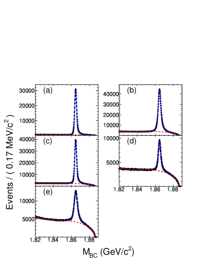
Figure 1: Distributions of the beam energy constrained masses of the $Kn\pi$ ($n$ = 1, 2, 3 or 4) combinations for the 5 single $\bar{D}^{0}$ tag modes: (a) $K^{+}\pi^{-}$, (b) $K^{+}\pi^{-}\pi^{0}$, (c) $K^{+}\pi^{-}\pi^{-}\pi^{+}$, (d) $K^{+}\pi^{-}\pi^{-}\pi^{+}\pi^{0}$ and (e) $K^{+}\pi^{-}\pi^{0}\pi^{0}$.

Table 1: Summary of the single $\bar{D}^{0}$ tags and efficiencies for reconstruction of the single $\bar{D}^{0}$ tags, where $\Delta E$ gives the requirements on the energy difference between the measured $E_{Kn\pi}$ and beam energy $E_{\rm beam}$, while the $M_{\rm B}$ range defines the signal region of the single $\bar{D}^{0}$ tags. $N_{\rm tag}$ is the number of single $\bar{D}^{0}$ tags and $\epsilon_{\rm tag}$ is the efficiency for reconstruction of the single $\bar{D}^{0}$ tags.

Tag mode	$\Delta E$ (GeV)	$M_{\rm BC}$ range (GeV$/c^{2}$)	$N_{\rm tag}$	$\epsilon_{\rm tag}$ (%)
$K^{+}\pi^{-}$	$(-0.049,0.044)$	$(1.860,1.875)$	$~{}567083\pm 848~{}$	$70.29\pm 0.07$
$K^{+}\pi^{-}\pi^{0}$	$(-0.071,0.052)$	$(1.858,1.875)$	$1094081\pm 1692$	$36.80\pm 0.03$
$K^{+}\pi^{-}\pi^{-}\pi^{+}$	$(-0.043,0.043)$	$(1.860,1.875)$	$~{}700061\pm 1121$	$39.57\pm 0.04$
$K^{+}\pi^{-}\pi^{-}\pi^{+}\pi^{0}$	$(-0.067,0.066)$	$(1.858,1.875)$	$~{}158367\pm 749~{}$	$15.95\pm 0.08$
$K^{+}\pi^{-}\pi^{0}\pi^{0}$	$(-0.082,0.050)$	$(1.858,1.875)$	$~{}273725\pm 2859$	$15.78\pm 0.08$
Sum			$2793317\pm 3684$

IV.3 Selection of $D^{0}\rightarrow K^{-}e^{+}\nu_{e}$ and $D^{0}\rightarrow\pi^{-}e^{+}\nu_{e}$

The $D^{0}\to K^{-}e^{+}\nu_{e}$ and $D^{0}\to\pi^{-}e^{+}\nu_{e}$ event candidates are selected from the tracks recoiling against the single $\bar{D}^{0}$ tags. To select the $D^{0}\to K^{-}e^{+}\nu_{e}$ and $D^{0}\to\pi^{-}e^{+}\nu_{e}$ events, it is required that there are only two oppositely charged tracks, one of which is identified as a positron and the other as a kaon or a pion. The combined confidence level $CL_{K}$ ($CL_{\pi}$) for the $K$ ($\pi$) hypothesis is required to be greater than $CL_{\pi}$ ($CL_{K}$) for kaon (pion) candidates. For positron identification, the combined confidence level ($CL_{e}$), calculated for the $e$ hypothesis using the $dE/dx$, TOF and EMC measurements (deposited energy and shape of the electromagnetic shower), is required to be greater than $0.1\%$, and the ratio $CL_{e}/(CL_{e}+CL_{\pi}+CL_{K})$ is required to be greater than $0.8$. We include the 4-momenta of near-by photons with the direction of the positron momentum to partially account for final-state-radiation energy losses (FSR recovery). In addition, to suppress fake photon background it is required that the maximum energy of any unused photon in the recoil system, $E_{\gamma,\rm max}$, be less than 300 MeV.

Since the neutrino escapes detection, the kinematic variable

$$U_{\rm miss}\equiv E_{\rm miss}-|\vec{p}_{\rm miss}|$$ (IV.6)

is used to obtain the information about the missing neutrino, where $E_{\rm miss}$ and $\vec{p}_{\rm miss}$ are, respectively, the total missing energy and momentum in the event, computed from

$$E_{\rm miss}=E_{\rm beam}-E_{h^{-}}-E_{e^{+}},$$ (IV.7)

where $E_{h^{-}}$ and $E_{e^{+}}$ are the measured energies of the hadron and the positron, respectively. The $\vec{p}_{\rm miss}$ is calculated by

$$\vec{p}_{\rm miss}=\vec{p}_{D^{0}}-\vec{p}_{h^{-}}-\vec{p}_{e^{+}},$$ (IV.8)

where $\vec{p}_{D^{0}}$, $\vec{p}_{h^{-}}$ and $\vec{p}_{e^{+}}$ are the momenta of the $D^{0}$ meson, the hadron and the positron, respectively. The 3-momentum $\vec{p}_{D^{0}}$ of the $D^{0}$ meson is computed by

$$\vec{p}_{D^{0}}=-\hat{p}_{\rm tag}\sqrt{E_{\rm beam}^{2}-m_{D^{0}}^{2}},$$ (IV.9)

where $\hat{p}_{\rm tag}$ is the direction of the momentum of the single $\bar{D}^{0}$ tag. If the daughter particles from a semileptonic decay are correctly identified, $U_{\rm miss}$ is zero, since only one neutrino is missing.

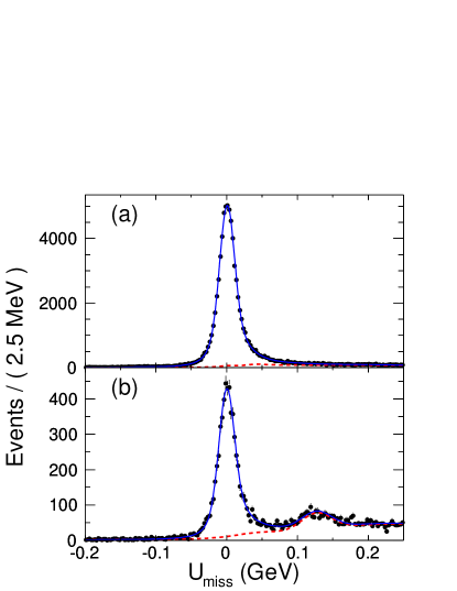
Figure 2: $U_{\rm miss}$ distributions of events for (a) $\bar{D}^{0}$ tags vs. $D^{0}\rightarrow K^{-}e^{+}\nu_{e}$, and for (b) $\bar{D}^{0}$ tags vs. $D^{0}\rightarrow\pi^{-}e^{+}\nu_{e}$, where the dots with error bars show the data, the solid lines show the best fit to the data, and the dashed lines show the background shapes estimated by analyzing the “cocktail vs. cocktail $D\bar{D}$ process” Monte Carlo events and the “non-$D\bar{D}$ process” Monte Carlo events (see text for more details).

Figures 2 (a) and (b) show the $U_{\rm miss}$ distributions for the $D^{0}\to K^{-}e^{+}\nu_{e}$ and $D^{0}\to\pi^{-}e^{+}\nu_{e}$ candidate events, respectively. In both cases, most of the events are from the $D^{0}\to K^{-}e^{+}\nu_{e}$ and $D^{0}\to\pi^{-}e^{+}\nu_{e}$ decays. Backgrounds from $D\bar{D}$ processes include mistagged $\bar{D}^{0}$ and $D^{0}$ decays other than the semileptonic decay in question. Other backgrounds are from “non-$D\bar{D}$ process” processes. From the simulated “cocktail vs. cocktail $D\bar{D}$ process” events, we find that the $D\bar{D}$ background events are mostly from $D^{0}\to K^{-}\pi^{0}e^{+}\nu_{e}$, $D^{0}\to K^{-}\mu^{+}\nu_{\mu}$ and $D^{0}\to\pi^{-}e^{+}\nu_{e}$ selected as $D^{0}\to K^{-}e^{+}\nu_{e}$, and $D^{0}\to\pi^{-}\pi^{0}e^{+}\nu_{e}$, $D^{0}\to K^{-}e^{+}\nu_{\mu}$ and $D^{0}\to\pi^{-}\mu^{+}\nu_{\mu}$ selected as $D^{0}\to\pi^{-}e^{+}\nu_{e}$. Backgrounds from “non-$D\bar{D}$” processes include the ISR (Initial State Radiation) return to the $\psi(3686)$ and $J/\psi$, continuum light hadron production, $\psi(3770)\rightarrow{\rm non}-D\bar{D}$ decays and $e^{+}e^{-}\rightarrow\tau^{+}\tau^{-}$ events. The levels of these backgrounds events are estimated by analyzing the corresponding simulated event samples.

Because of ISR and FSR (Final State Radiation), the signal $U_{\rm miss}$ distributions are not Gaussian; instead, the $U_{\rm miss}$ distributions have Gaussian cores with long tails at both the lower and the higher sides of the distributions. To obtain the numbers of the signal events for these two semileptonic decays, we fit these distributions with an empirical function that includes these tails.

We use the same probability density function as CLEO cleo-c_Phys_Rev_D79_052010_y2009 for $U_{\rm miss}$,

$$f(x)=\left\{\begin{array}[]{ll}a_{1}\left(\frac{n_{1}}{\alpha_{1}}-\alpha_{1}+x\right)^{-n_{1}}&{\rm if~{}}x\geq\alpha_{1}\\ \exp(-x^{2}/2)&{\rm if~{}}-\alpha_{2}\leq x<\alpha_{1},\\ a_{2}\left(\frac{n_{2}}{\alpha_{2}}-\alpha_{2}-x\right)^{-n_{2}}&{\rm if~{}}x<-\alpha_{2}\end{array}\right.$$ (IV.10)

where $x\equiv(U_{\rm miss}-m)/\sigma$, $m$ and $\sigma$ are the mean value and standard deviation of the Gaussian distribution, respectively. In Eq. (IV.10), $a_{1}\equiv(n_{1}/\alpha_{1})^{n_{1}}e^{-\alpha^{2}_{1}/2}$, and $a_{2}\equiv(n_{2}/\alpha_{2})^{n_{2}}e^{-\alpha^{2}_{2}/2}$, where $\alpha_{1}$, $\alpha_{2}$, $n_{1}$ and $n_{2}$ are parameters describing the tails of the signal function, determined from fits to the simulated $U_{\rm miss}$ distributions of signal Monte Carlo events.

To account for differences between data and Monte Carlo, we fit the data using the Monte Carlo determined $f(x)$ distribution convolved with a Gaussian function with free mean and width. The background function is formed from histograms of $U_{\rm miss}$ distributions for background events from the “cocktail vs. cocktail” $D\bar{D}$ and “non-$D\bar{D}$” simulated event samples. The normalizations of the signal and background are free parameters in the fits to the data.

The results of the fits to the two $U_{\rm miss}$ distributions are shown in Figs. 2 (a) and (b); the fitted yields of signal events are

$$N_{\rm observed}(D^{0}\to K^{-}e^{+}\nu_{e})=70727.0\pm 278.3$$ (IV.11)

and

$$N_{\rm observed}(D^{0}\to\pi^{-}e^{+}\nu_{e})=6297.1\pm 86.8.$$ (IV.12)

In Fig. 2 (a) and (b), the solid lines show the best fits to the data, while the dashed lines show the background.

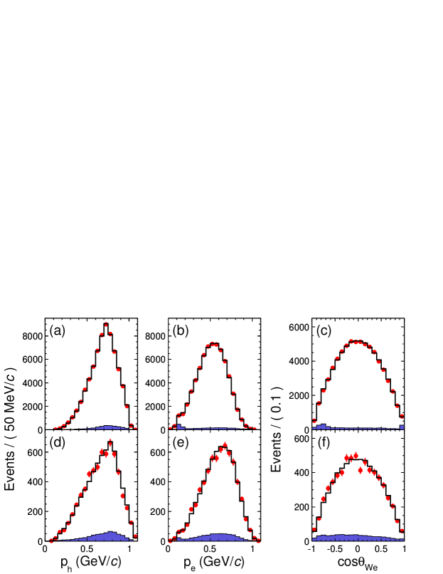
Figure 3: Distributions of particle momenta and $\cos\theta_{We}$ from $D^{0}\rightarrow K^{-}e^{+}\nu_{e}$ and $D^{0}\rightarrow\pi^{-}e^{+}\nu_{e}$ semileptonic decays, where (a) and (b) are the momenta of kaon and positron from $D^{0}\rightarrow K^{-}e^{+}\nu_{e}$, respectively, (d) and (e) are the momenta of pion and positron from $D^{0}\rightarrow\pi^{-}e^{+}\nu_{e}$, respectively; (c) and (f) are the distributions of $\cos\theta_{We}$ for $D^{0}\to K^{-}e^{+}\nu_{e}$ and $D^{0}\to\pi^{-}e^{+}\nu_{e}$, respectively; these events satisfy $-0.06<U_{\rm miss}<0.06~{}\rm GeV$. The solid histograms are Monte Carlo simulated signal plus background; the shaded histograms are Monte Carlo simulated background only.

To gain confidence in the quality of the Monte Carlo simulation, we examine the momentum distributions of the kaon, the pion and the positron as well as $\cos\theta_{We}$ from the semileptonic decays of $D^{0}\rightarrow K^{-}e^{+}\nu_{e}$ and $D^{0}\rightarrow\pi^{-}e^{+}\nu_{e}$, where $\theta_{We}$ is the angle between the direction of the virtual $W^{+}$ boson in the $D^{0}$ rest frame and the three-momentum of the positron in the $W^{+}$ rest frame. These distributions are shown in Figs. 3 (a)-(f), respectively, where the dots with error bars are for the data, the solid histograms are for the full Monte Carlo simulation and the shaded histograms show the Monte Carlo simulated backgrounds only.

V Measurements of Absolute Decay Branching Fractions

V.1 Efficiency for reconstruction of semileptonic decays

To determine the efficiency $\epsilon(D^{0}\rightarrow h^{-}e^{+}\nu_{e})$ for reconstruction of each of the two semileptonic decays for each single tag mode, “Signal” Monte Carlo event samples of $\psi(3770)\to D^{0}\bar{D}^{0}$ decays, where the $D^{0}$ meson is set to decay to the $h^{-}e^{+}\nu_{e}$ final state in question and the $\bar{D}^{0}$ meson is set to decay to each of the five single $\bar{D}^{0}$ tag modes, are generated and simulated with the BESIII software package. By subjecting these simulated events to the same requirements that are applied to the data we obtain the reconstruction efficiencies $\epsilon_{{\rm tag},D^{0}\to h^{-}e^{+}\nu_{e}}$ for simultaneously finding the $D^{0}$ meson semileptonic decay and the single $\bar{D}^{0}$ tag in the same event; these are given in Tab. 2.

Table 2: Double tag efficiencies for reconstruction of “$\bar{D}^{0}_{\rm tag}$ vs. $D^{0}\to h^{-}e^{+}\nu_{e}$” and overall efficiencies for reconstruction of $D^{0}\to h^{-}e^{+}\nu_{e}$ in the recoil side of $\bar{D}^{0}$ tags.

Tag mode	$\epsilon_{{\rm tag},D^{0}\to K^{-}e^{+}\nu_{e}}$	$\epsilon_{{\rm tag},D^{0}\to\pi^{-}e^{+}\nu_{e}}$	$\epsilon_{\rm MC}(D^{0}\to K^{-}e^{+}\nu_{e})$	$\epsilon_{\rm MC}(D^{0}\to\pi^{-}e^{+}\nu_{e})$
$K^{+}\pi^{-}$	$0.4566\pm 0.0014$	$0.4995\pm 0.0014$	$0.6496\pm 0.0021$	$0.7106\pm 0.0021$
$K^{+}\pi^{-}\pi^{0}$	$0.2685\pm 0.0006$	$0.2927\pm 0.0007$	$0.7296\pm 0.0017$	$0.7954\pm 0.0020$
$K^{+}\pi^{-}\pi^{-}\pi^{+}$	$0.2666\pm 0.0008$	$0.2897\pm 0.0008$	$0.6737\pm 0.0021$	$0.7321\pm 0.0022$
$K^{+}\pi^{-}\pi^{-}\pi^{+}\pi^{0}$	$0.1260\pm 0.0008$	$0.1363\pm 0.0008$	$0.7900\pm 0.0064$	$0.8545\pm 0.0066$
$K^{+}\pi^{-}\pi^{0}\pi^{0}$	$0.1331\pm 0.0007$	$0.1467\pm 0.0007$	$0.8435\pm 0.0062$	$0.9297\pm 0.0065$
Average			$0.7140\pm 0.0012$	$0.7788\pm 0.0013$

Due to their low multiplicity, it is usually easier to reconstruct $\bar{D}^{0}$ tags in semileptonic events than in typical $D^{0}\bar{D}^{0}$ events (tag bias). In addition, the size of the tag bias is correlated with the multiplicity of the tag mode. In consequence the overall efficiencies shown in Tab. 2 vary greatly from the $\bar{D}^{0}\to K^{-}\pi^{+}$ mode to the $\bar{D}^{0}\to K^{-}\pi^{+}\pi^{+}\pi^{-}$ and $\bar{D}^{0}\to K^{-}\pi^{+}\pi^{0}\pi^{0}$ modes.

The last row in Tab. 2 gives the overall efficiency which is obtained by weighting the individual efficiencies for each of the five single $\bar{D}^{0}$ tags by the corresponding yield shown in Tab. 1.

There are small differences in efficiencies for finding a charged particle and for identifying the type of the charged particle between the data and Monte Carlo events that are discussed below in Section V.3. To take these differences into account, the overall efficiencies $\epsilon_{\rm MC}(D^{0}\to K^{-}e^{+}\nu_{e})$ and $\epsilon_{\rm MC}(D^{0}\to\pi^{-}e^{+}\nu_{e})$ are corrected by the multiplicative factors of

$$f_{\rm corr}^{\rm trk+PID}=\left\{\begin{array}[]{ll}1.0118&{\rm for}~{}D^{0}\to K^{-}e^{+}\nu_{e},\\ 0.9814&{\rm for}~{}D^{0}\to\pi^{-}e^{+}\nu_{e}.\end{array}\right.$$ (V.1)

After making these corrections, we obtain the “true” overall efficiencies for reconstruction of these two semileptonic decays,

$$\epsilon(D^{0}\to K^{-}e^{+}\nu_{e})=0.7224\pm 0.0012,$$ (V.2)

and

$$\epsilon(D^{0}\to\pi^{-}e^{+}\nu_{e})=0.7643\pm 0.0013.$$ (V.3)

V.2 Decay branching fraction

Inserting the number of the single $\bar{D}^{0}$ tags, the numbers of the signal events for these two $D^{0}$ semileptonic decays observed in the recoil of the single $\bar{D}^{0}$ tags together with corresponding efficiency into Eq.(IV.3), we obtain the absolute decay branching fractions

$$\mathcal{B}(D^{0}\to K^{-}e^{+}\nu_{e})=(3.505\pm 0.014\pm 0.033)\%$$ (V.4)

and

$$\mathcal{B}(D^{0}\to\pi^{-}e^{+}\nu_{e})=(0.295\pm 0.004\pm 0.003)\%,$$ (V.5)

where the first errors are statistical and the second systematic. The sources of systematic uncertainties in the measured decay branching fractions are discussed in the next subsection.

V.3 Systematic uncertainties in measured branching fractions

Table 3 lists the sources of the systematic uncertainties in the measured semileptonic branching fractions. We discuss each of these sources in the following.

Table 3: Sources of the systematic uncertainties in the measured branching fractions for $D^{0}\rightarrow K^{-}e^{+}\nu_{e}$ and $D^{0}\rightarrow\pi^{-}e^{+}\nu_{e}$.

	Systematic uncertainty (%)
Source	$K^{-}e^{+}\nu_{e}$	$\pi^{-}e^{+}\nu_{e}$
Number of $\bar{D}^{0}$ tags	0.50	0.50
Tracking for $e^{+}$	0.19	0.15
Tracking for $K^{-}$	0.42	—
Tracking for $\pi^{-}$	—	0.28
PID for $e^{+}$	0.16	0.14
PID for $K^{-}$	0.10	—
PID for $\pi^{-}$	—	0.19
$E_{\gamma,{\rm max}}$ cut	0.10	0.10
Fit to $U_{\rm miss}$	0.48	0.50
Form factor structure	0.10	0.10
FSR recovery	0.30	0.30
Finite MC statistics	0.17	0.17
Single tag cancelation	0.12	0.12
Total	0.94	0.90

V.3.1 Uncertainty in number of $\bar{D}^{0}$ tags

To estimate the uncertainty in the number of single $\bar{D}^{0}$ tags, we repeat the fits to the $M_{\rm BC}$ distributions by varying the bin size, fit range and background functions. We also investigate the contribution arising from possible differences in the $\pi^{0}$ fake rates between data and Monte Carlo simulation. Finally, we assign a systematic uncertainty of 0.5% to the number of $\bar{D}^{0}$ tags.

V.3.2 Uncertainty in tracking efficiency

The uncertainties for finding a charged track are estimated by comparing the efficiencies for reconstructing the positron, kaon and pion in data and Monte Carlo events.

Using radiative Bhabha scattering events selected from the data and simulated radiative Bhabha scattering events, we measure the difference in efficiencies for finding a positron between data and simulation. Considering both the $\cos\theta$, where $\theta$ is the polar angle of the positron, and momentum distributions of the positrons, we obtain two-dimensional weighted-average efficiency differences ($\epsilon_{\rm data}/\epsilon_{\rm MC}-1$) of $(0.22\pm 0.19)\%$ and $(0.11\pm 0.15)\%$. These translate uncertainties on the decay branching fractions of $0.19\%$ and $0.15\%$ for $D^{0}\to K^{-}e^{+}\nu_{e}$ and $D^{0}\to\pi^{-}e^{+}\nu_{e}$ decays, respectively.

The efficiencies for finding a charged kaon and a charged pion are determined by analyzing doubly tagged $D\bar{D}$ decay events. In the selection of the doubly tagged $D\bar{D}$ decay events, we exclude one charged kaon or one charged pion track and examine the variable $M^{2}_{{\rm miss}~{}K~{}{\rm or}~{}\pi}$, defined as the difference between the missing energy squared $E^{2}_{\rm miss}$ and the missing momentum squared $p^{2}_{\rm miss}$ of the selected $D\bar{D}$ decay events. By analyzing these $M^{2}_{{\rm miss}~{}K~{}{\rm or}~{}\pi}$ variables for both the data and the simulated “cocktail vs. cocktail $D\bar{D}$ process” Monte Carlo events, we find the differences in efficiencies for reconstructing a charged kaon or a charged pion between the data and the Monte Carlo events as a function of the charged particle momentum. Considering the momentum distributions of the kaon and pion from these two semileptonic decays, we obtain the magnitudes of systematic differences and their uncertainties of the track reconstruction efficiencies. The level of uncertainties in the corrections for these differences in measurements of the decay branching fractions and partial decay rates (see Section VI) are $0.42\%$ and $0.28\%$ for charged kaons and pions, respectively.

V.3.3 Uncertainty in particle identification

The differences in efficiencies for identifying a positron between the data and the Monte Carlo samples depend not only on the momentum of the positron, but also on $\cos\theta$. Considering both of these for our signal positrons, we obtain a weighted-average difference in efficiency for identifying the positron from the two semileptonic decays. After making correction for these differences in efficiencies for identifying the positrons, we obtain a systematic uncertainty of $0.16\%$ ($0.14\%$) on the $K^{-}(\pi^{-})e^{+}\nu_{e}$ mode from this source.

The systematic uncertainties associated with the efficiencies for identifying a charged kaon and a charged pion are estimated using the missing mass square techniques discussed above. Taking into account the momentum distributions of the charged particles from the two semileptonic modes, we correct for the momentum-weighted efficiency differences for identifying the kaon and the pion, and we assign systematic uncertainties of $0.10\%$ and $0.19\%$ for charged kaons and pions, respectively.

V.3.4 Uncertainty in $E_{\gamma,\rm max}$ cut

The uncertainty associated with the $E_{\gamma,\rm max}$ requirement on the events is estimated by analyzing doubly tagged $D\bar{D}$ events with hadronic decay modes. With these events, we examine the fake photons from the EMC measurements. By analyzing these selected samples from both the data and the simulated Monte Carlo events, we find that the magnitude of difference in the number of fake photons between the data and the Monte Carlo events is $0.10\%$, which is set as the systematic uncertainty due to this source.

V.3.5 Uncertainty in fit to $U_{\rm miss}$ distribution

To estimate the systematic uncertainty in the numbers of signal events due to the fit to the $U_{\rm miss}$ distribution, we vary the bin size and the tail parameters of the signal function. We then repeat the fits to the $U_{\rm miss}$ distributions, and combine the changes in the yields in quadrature to obtain the systematic uncertainty. Since the background function is formed from many background modes with fixed relative normalizations, we also vary the relative contributions of several of the largest background modes based on the uncertainties in their branching fractions and the uncertainties in the rates of misidentifying a hadron (muon) as an electron. Finally we find that the relative sizes of this systematic uncertainty are 0.48% and 0.50% for $D^{0}\to K^{-}e^{+}\nu_{e}$ and $D^{0}\to\pi^{-}e^{+}\nu_{e}$, respectively.

V.3.6 Uncertainty in form factors

In order to estimate the systematic uncertainty associated with the form factor used to generate signal events in the Monte Carlo simulation, we re-weight the signal Monte Carlo events so that their $q^{2}$ distributions match the measured spectra. We then re-measure the branching fraction (partial decay rates in different $q^{2}$ bins) with the new weighted efficiency (efficiency matrix). The maximum relative changes in branching fraction (partial decay rates in different $q^{2}$ bins) is $0.05\%$. To be conservative, we assign a relative systematic uncertainty of $0.10\%$ to the branching fraction measurements for $D^{0}\to K^{-}e^{+}\nu_{e}$ and $D^{0}\to\pi^{-}e^{+}\nu_{e}$ decays.

V.3.7 Uncertainty in FSR recovery

The difference between the measured branching fraction obtained with the FSR recovery of the positron momentum and the one obtained without the FSR recovery is assigned as the most conservative systematic uncertainty due to FSR recovery. We find the magnitude of this difference to be $0.30\%$ for both $D^{0}\to K^{-}e^{+}\nu_{e}$ and $D^{0}\to\pi^{-}e^{+}\nu_{e}$ decays.

V.3.8 Uncertainty due to finite Monte Carlo statistics

The uncertainties associated with the finite Monte Carlo statistics are $0.17\%$ for both $D^{0}\rightarrow K^{-}e^{+}\nu_{e}$ and $D^{0}\rightarrow\pi^{-}e^{+}\nu_{e}$.

V.3.9 Uncertainty due to single tag cancelation

Most of the systematic uncertainties arising from the selection of single $\bar{D}^{0}$ tags are canceled due to the double tag technique. The un-canceled systematic error of MDC tracking, particle identification and $\pi^{0}$ selection in single tag selection is estimated by $\left(\sum_{\rm tag}(\epsilon^{\prime}_{\rm tag}/\epsilon_{\rm tag}-1)\times 0.25\delta_{\rm tag}\times N_{\rm tag}\right)/\left(\sum_{\rm tag}N_{\rm tag}\right)$, where $\epsilon^{\prime}_{\rm tag}$ and $\epsilon_{\rm tag}$ are the efficiencies of reconstructing single $\bar{D}^{0}$ tags obtained by analyzing the Monte Carlo events of $\bar{D}^{0}\to{\rm tag}$ vs. $D^{0}\to h^{-}e^{+}\nu_{e}$ and $\bar{D}^{0}\to{\rm tag}$ vs. $D^{0}\to anything$ after mixing all the simulated backgrounds, respectively; $N_{\rm tag}$ is the number of single $\bar{D}^{0}$ tags reconstructed in data; $\delta_{\rm tag}$ is the total systematic error of MDC tracking, particle identification and $\pi^{0}$ selection in single tag selection. Since no efficiency correction is made in the single tag selection, the uncertainty in MDC tracking (or particle identification) for charged kaon or pion is taken to be 1.0% per track, and the uncertainty in $\pi^{0}$ selection is taken to be 2.0% per $\pi^{0}$. For each single $\bar{D}^{0}$ tag mode, the uncertainty in MDC tracking, particle identification or $\pi^{0}$ selection are added linearly separately, and then they are added in quadrature to obtain the total systematic error in the single $\bar{D}^{0}$ tag selection. Finally, we assign a systematic uncertainty of 0.12% for the branching fraction measurements.

V.4 Comparison with other measurements

A comparison of our measured branching fractions for $D^{0}\rightarrow K^{-}e^{+}\nu_{e}$ and $D^{0}\rightarrow\pi^{-}e^{+}\nu_{e}$ decays with those previously measured by the MARK-III mark-iii , CLEO cleo , BES-II bes2_plb597_p39_2004 , CLEO cleo-c_prl95_181802_y2005 ; cleo-c_Phys_Rev_D79_052010_y2009 ; cleo-c_Phys_Rev_D80_032005_y2009 (at the CLEO-c experiment) and BABAR BaBar_Phys_Rev_D76_p052005_y2007 ; BaBar_D0topienu Collaborations as well as the world average given by the PDG pdg2014 is given in Table 4. Our measured branching fractions for these two decays are in excellent agreement with the experimental results obtained by other experiments, but are more precise. In the table, we also compare our branching fraction measurements to theoretical predictions for these two semileptonic decays. The precision of our measured branching fractions are much higher than those of the LQCD lqcd_prl_94_011601 ; LQCD_2 , the QCD sum rule QCDSR and the LCSR LCSR_2 predictions.

Table 4: Comparison of the measured $\mathcal{B}(D^{0}\to K^{-}e^{+}\nu_{e})$ and $\mathcal{B}(D^{0}\to\pi^{-}e^{+}\nu_{e})$ values with those measured by other experiments and theoretical predictions based on QCD and the world-average value of $\tau_{D^{0}}$.

Experiment/Theory	$\mathcal{B}(D^{0}\to K^{-}e^{+}\nu_{e})$ (%)	$\mathcal{B}(D^{0}\to\pi^{-}e^{+}\nu_{e})$ (%)
PDG2014 pdg2014	$3.55\pm 0.05$	$0.289\pm 0.008$
MARK-III mark-iii	$3.4\pm 0.5\pm 0.4$	$0.39^{+0.23}_{-0.11}\pm 0.04$
CLEO cleo	$3.82\pm 0.11\pm 0.25$
BES-II bes2_plb597_p39_2004	$3.82\pm 0.40\pm 0.27$	$0.33\pm 0.13\pm 0.03$
CLEO-c cleo-c_Phys_Rev_D80_032005_y2009	$3.50\pm 0.03\pm 0.04$	$0.288\pm 0.008\pm 0.003$
Belle bell_Phys_RevLett_97_p061804_y2006	$3.45\pm 0.07\pm 0.20$	$0.255\pm 0.019\pm 0.016$
BABAR BaBar_Phys_Rev_D76_p052005_y2007 ; BaBar_D0topienu	$3.522\pm 0.027\pm 0.045\pm 0.065$	$0.2770\pm 0.0068\pm 0.0092\pm 0.0037$
BESIII (this experiment)	$3.505\pm 0.014\pm 0.033$	$0.295\pm 0.004\pm 0.003$
LQCD  lqcd_prl_94_011601	$3.77\pm 0.29\pm 0.74$	$0.316\pm 0.025\pm 0.070$
LQCD  LQCD_2	$2.99\pm 0.45\pm 0.74$	$0.24\pm 0.06$
QCD SR QCDSR	$2.7\pm 0.6$
LCSR LCSR_2	$3.9\pm 1.2$	$0.30\pm 0.09$

VI Differential decay rates

The differential decay rate $d\Gamma/dq^{2}$ for $D^{0}\to K^{-}(\pi^{-})e^{+}\nu_{e}$ is given by Eq. (I.1). The form factor $f_{+}^{K(\pi)}(q^{2})$ can be extracted from measurements of $d\Gamma/dq^{2}$. Such measurements are obtained from the event rates in bins of $q^{2}$ ranging from $q^{2}_{i}-0.5\Delta q^{2}$ to $q^{2}_{i}+0.5\Delta q^{2}$, where $\Delta q^{2}$ is the bin width and $i$ is the bin number.

VI.1 Measurement of differential decay rates

The $q^{2}$ value is given by

$$q^{2}=(E_{e}+E_{\nu})^{2}-(\vec{p}_{e}+\vec{p}_{\nu})^{2},$$ (VI.1)

where $E_{e}$ and $\vec{p}_{e}$ are the measured energy and momentum of the positron, $E_{\nu}$ and $\vec{p}_{\nu}$ are the energy and momentum of the missing neutrino:

$$E_{\nu}=E_{\rm miss},$$ (VI.2)

$$\vec{p}_{\nu}=E_{\rm miss}\hat{p}_{\rm miss}.$$ (VI.3)

For the $D^{0}\rightarrow K^{-}e^{+}\nu_{e}$ differential rate, we divide the candidates for the decays into 18 $q^{2}$ bins. For the $D^{0}\to\pi^{-}e^{+}\nu_{e}$ mode, which has fewer events, we use 14 $q^{2}$ bins. The first columns of Tables 5 and 6 give the range of each $q^{2}$ bin for $D^{0}\to K^{-}e^{+}\nu_{e}$ and $D^{0}\to\pi^{-}e^{+}\nu_{e}$, respectively.

Table 5: Summary of the range of each $q^{2}$ bin, the number of the observed events $N_{\rm observed}$, the number of produced events $N_{\rm produced}$, and the partial decay rate $\Delta\Gamma$ in each $q^{2}$ bin for $D^{0}\to K^{-}e^{+}\nu_{e}$ decays.

$q^{2}$ (GeV${}^{2}/c^{4})$	$N_{\rm observed}$	$N_{\rm produced}$	$\Delta\Gamma$ (ns-1)
(0.0, 0.1)	$7876.1\pm 94.2$	$10094.9\pm 132.3$	$8.812\pm 0.116$
(0.1, 0.2)	$7504.3\pm 90.5$	$10015.4\pm 140.8$	$8.743\pm 0.123$
(0.2, 0.3)	$6940.5\pm 87.2$	$~{}9502.6\pm 142.0$	$8.295\pm 0.124$
(0.3, 0.4)	$6376.0\pm 83.4$	$~{}8667.9\pm 138.6$	$7.567\pm 0.121$
(0.4, 0.5)	$6139.8\pm 81.9$	$~{}8575.9\pm 137.7$	$7.486\pm 0.120$
(0.5, 0.6)	$5460.5\pm 77.1$	$~{}7384.0\pm 128.1$	$6.446\pm 0.112$
(0.6, 0.7)	$5120.3\pm 74.7$	$~{}7101.8\pm 125.8$	$6.200\pm 0.110$
(0.7, 0.8)	$4545.5\pm 70.5$	$~{}6322.2\pm 120.2$	$5.519\pm 0.105$
(0.8, 0.9)	$4159.4\pm 67.1$	$~{}5760.3\pm 113.3$	$5.028\pm 0.099$
(0.9, 1.0)	$3680.7\pm 63.2$	$~{}5183.5\pm 107.6$	$4.525\pm 0.094$
(1.0, 1.1)	$3199.6\pm 58.9$	$~{}4550.0\pm 100.2$	$3.972\pm 0.087$
(1.1, 1.2)	$2637.1\pm 53.5$	$~{}3810.2\pm 92.4~{}$	$3.326\pm 0.081$
(1.2, 1.3)	$2239.1\pm 49.4$	$~{}3239.1\pm 84.3~{}$	$2.828\pm 0.074$
(1.3, 1.4)	$1752.1\pm 43.9$	$~{}2621.2\pm 77.3~{}$	$2.288\pm 0.067$
(1.4, 1.5)	$1301.0\pm 37.7$	$~{}1989.4\pm 67.4~{}$	$1.737\pm 0.059$
(1.5, 1.6)	$927.5\pm 32.0$	$~{}1505.1\pm 59.0~{}$	$1.314\pm 0.052$
(1.6, 1.7)	$541.3\pm 24.6$	$~{}~{}983.4\pm 50.3~{}$	$0.858\pm 0.044$
(1.7, $q^{2}_{\rm max}$)	$188.2\pm 15.1$	$~{}~{}434.2\pm 39.6~{}$	$0.379\pm 0.035$

Table 6: Summary of the range of each $q^{2}$ bin, the number of the observed events $N_{\rm observed}$, the number of produced events $N_{\rm produced}$, and the partial decay rate $\Delta\Gamma$ in each $q^{2}$ bin for $D^{0}\to\pi^{-}e^{+}\nu_{e}$ decays.

$q^{2}$ (GeV${}^{2}/c^{4}$)	$N_{\rm observed}$	$N_{\rm produced}$	$\Delta\Gamma$ (ns-1)
(0.0, 0.2)	$814.4\pm 30.9$	$1066.9\pm 43.2$	$0.931\pm 0.038$
(0.2, 0.4)	$697.2\pm 28.7$	$~{}935.1\pm 42.8$	$0.816\pm 0.037$
(0.4, 0.6)	$634.6\pm 27.7$	$~{}836.6\pm 41.3$	$0.730\pm 0.036$
(0.6, 0.8)	$654.6\pm 27.8$	$~{}850.1\pm 40.6$	$0.742\pm 0.035$
(0.8, 1.0)	$643.2\pm 27.3$	$~{}840.2\pm 39.9$	$0.733\pm 0.035$
(1.0, 1.2)	$578.6\pm 26.3$	$~{}744.6\pm 37.7$	$0.650\pm 0.033$
(1.2, 1.4)	$509.9\pm 24.7$	$~{}651.1\pm 35.1$	$0.568\pm 0.031$
(1.4, 1.6)	$438.6\pm 23.2$	$~{}551.6\pm 32.8$	$0.481\pm 0.029$
(1.6, 1.8)	$412.6\pm 22.3$	$~{}534.7\pm 31.7$	$0.467\pm 0.028$
(1.8, 2.0)	$320.9\pm 19.8$	$~{}420.6\pm 28.6$	$0.367\pm 0.025$
(2.0, 2.2)	$245.8\pm 17.0$	$~{}324.0\pm 24.7$	$0.283\pm 0.022$
(2.2, 2.4)	$165.4\pm 14.1$	$~{}229.9\pm 21.7$	$0.201\pm 0.019$
(2.4, 2.6)	$93.6\pm 10.7$	$~{}129.2\pm 16.7$	$0.113\pm 0.015$
(2.6, $q^{2}_{\rm max}$)	$75.8\pm 10.0$	$~{}107.2\pm 15.0$	$0.094\pm 0.013$

Figure 4: Distributions of $U_{\rm miss}$ for $\bar{D}^{0}$ tags vs. $D^{0}\rightarrow K^{-}e^{+}\nu_{e}$ with the squared 4-momentum transfer $q^{2}$ filled in different $q^{2}$ bins. The dots with error bars show the data, the blue solid lines show the best fits to the data, while the red dashed lines show the background shapes.

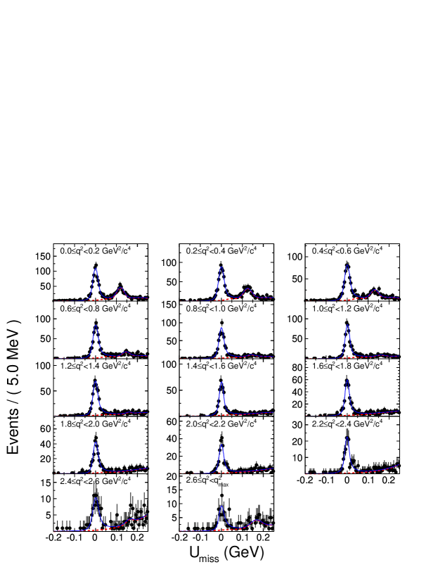
Figure 5: Distributions of $U_{\rm miss}$ for $\bar{D}^{0}$ tags vs. $D^{0}\rightarrow\pi^{-}e^{+}\nu_{e}$ with the squared 4-momentum transfer $q^{2}$ filled in different $q^{2}$ bins. The dots with error bars show the data, the blue solid lines show the best fits to the data, while the red dashed lines show the background shapes.

The points with error bars in Figs. 4 and 5 show the $U_{\rm miss}$ distributions for the $D^{0}\rightarrow K^{-}e^{+}\nu_{e}$ and $D^{0}\rightarrow\pi^{-}e^{+}\nu_{e}$ decays for each $q^{2}$ bin, respectively. Fits to these distributions that follow the procedure described in Section IV.3 give the signal yields $N_{\rm observed}$ for each $q^{2}$ bin. In these figures, the blue solid lines show the best fit to the data, while the red dashed lines show the background. In these fits, the background normalizations are left free.

To account for detection efficiency and detector resolution, the number of events $N^{i}_{\rm observed}$ observed in the $i$th $q^{2}$ bin is extracted from the relation

$$N^{i}_{\rm observed}=\sum_{j=1}^{N_{\rm bins}}\epsilon_{ij}N^{j}_{\rm produced},$$ (VI.4)

where $\epsilon_{ij}$ is the overall efficiency matrix that describes the efficiency and migration across $q^{2}$ bins.

The efficiency matrix element $\epsilon_{ij}$ is obtained by

$$\epsilon_{ij}=\frac{N^{\rm reconstructed}_{ij}}{N^{\rm generated}_{j}}\frac{1}{\epsilon_{\rm tag}}f_{{\rm corr},ij}^{\rm trk+PID},$$ (VI.5)

where $N^{\rm reconstructed}_{ij}$ is the number of signal Monte Carlo events generated in the $j$th $q^{2}$ bin and reconstructed in the $i$th $q^{2}$ bin, $N^{\rm generated}_{j}$ is the total number of the signal Monte Carlo events which are generated in the $j$th $q^{2}$ bin, $\epsilon_{\rm tag}$ is the single $\bar{D}^{0}$ tag efficiency, and $f_{{\rm corr},ij}^{\rm trk+PID}$ is the efficiency correction matrix for correcting the Monte Carlo deviations for tracking and particle identification efficiencies of each element of the efficiency matrix described above.

Table 7 presents the average overall efficiency matrix for the $D^{0}\to K^{-}e^{+}\nu_{e}$ mode. To produce this average overall efficiency matrix, we combine the efficiency matrices for each tag mode weighted by its yields shown in Tab. 1. The diagonal elements of the matrix give the overall efficiency for $D^{0}\rightarrow K^{-}e^{+}\nu_{e}$ decays to be reconstructed in the correct $q^{2}$ bin in the recoil of the single $\bar{D}^{0}$ tags, while the neighboring off-diagonal elements of the matrix give the overall efficiency for cross feed between different $q^{2}$ bins. Similarly, Table 8 presents the average overall efficiency matrix for the $D^{0}\to\pi^{-}e^{+}\nu_{e}$ channel.

Table 7: Weighted efficiency matrix $\epsilon_{ij}$ (in percent) for $D^{0}\to K^{-}e^{+}\nu_{e}$. The column gives the true $q^{2}$ bin $j$, while the row gives the reconstructed $q^{2}$ bin $i$.

$\epsilon_{ij}$	$1$	$2$	$3$	$4$	$5$	$6$	$7$	$8$	$9$	$10$	$11$	$12$	$13$	$14$	$15$	$16$	$17$	$18$
1	$71.62$	$5.39$	$0.70$	$0.31$	$0.11$	$0.03$	$0.01$	$0.00$	$0.01$	$0.00$	$0.00$	$0.00$	$0.00$	$0.00$	$0.00$	$0.00$	$0.00$	$0.00$
2	$2.54$	$65.14$	$6.31$	$0.86$	$0.42$	$0.15$	$0.02$	$0.01$	$0.01$	$0.00$	$0.00$	$0.00$	$0.00$	$0.00$	$0.00$	$0.00$	$0.00$	$0.00$
3	$0.05$	$3.19$	$62.49$	$6.53$	$0.84$	$0.37$	$0.10$	$0.05$	$0.01$	$0.02$	$0.00$	$0.00$	$0.00$	$0.01$	$0.00$	$0.02$	$0.00$	$0.00$
4	$0.02$	$0.09$	$3.61$	$61.47$	$7.07$	$0.79$	$0.31$	$0.09$	$0.01$	$0.00$	$0.01$	$0.01$	$0.00$	$0.00$	$0.00$	$0.00$	$0.00$	$0.00$
5	$0.01$	$0.02$	$0.11$	$3.64$	$60.77$	$6.93$	$0.88$	$0.29$	$0.08$	$0.01$	$0.01$	$0.03$	$0.00$	$0.00$	$0.00$	$0.00$	$0.00$	$0.00$
6	$0.00$	$0.03$	$0.05$	$0.10$	$3.98$	$61.58$	$6.81$	$0.80$	$0.27$	$0.08$	$0.01$	$0.03$	$0.00$	$0.00$	$0.01$	$0.00$	$0.00$	$0.00$
7	$0.01$	$0.01$	$0.01$	$0.05$	$0.14$	$4.16$	$60.75$	$6.71$	$0.66$	$0.27$	$0.04$	$0.02$	$0.02$	$0.00$	$0.00$	$0.00$	$0.00$	$0.00$
8	$0.00$	$0.00$	$0.02$	$0.01$	$0.05$	$0.16$	$4.12$	$60.04$	$6.70$	$0.75$	$0.22$	$0.04$	$0.04$	$0.02$	$0.00$	$0.00$	$0.00$	$0.00$
9	$0.00$	$0.00$	$0.01$	$0.03$	$0.01$	$0.05$	$0.18$	$4.12$	$60.61$	$6.64$	$0.75$	$0.17$	$0.03$	$0.03$	$0.01$	$0.00$	$0.00$	$0.00$
10	$0.00$	$0.01$	$0.00$	$0.00$	$0.02$	$0.05$	$0.05$	$0.17$	$4.01$	$59.99$	$6.38$	$0.62$	$0.12$	$0.04$	$0.03$	$0.00$	$0.00$	$0.00$
11	$0.00$	$0.00$	$0.01$	$0.00$	$0.01$	$0.01$	$0.04$	$0.09$	$0.20$	$3.91$	$59.97$	$5.84$	$0.62$	$0.10$	$0.01$	$0.02$	$0.00$	$0.00$
12	$0.00$	$0.00$	$0.00$	$0.00$	$0.00$	$0.01$	$0.02$	$0.03$	$0.05$	$0.15$	$3.90$	$59.02$	$5.61$	$0.46$	$0.09$	$0.04$	$0.00$	$0.00$
13	$0.00$	$0.00$	$0.00$	$0.00$	$0.00$	$0.00$	$0.00$	$0.00$	$0.03$	$0.12$	$0.20$	$3.82$	$59.59$	$5.15$	$0.47$	$0.11$	$0.03$	$0.00$
14	$0.00$	$0.00$	$0.00$	$0.00$	$0.00$	$0.00$	$0.00$	$0.00$	$0.02$	$0.03$	$0.10$	$0.23$	$3.63$	$57.71$	$5.06$	$0.34$	$0.00$	$0.00$
15	$0.00$	$0.00$	$0.00$	$0.00$	$0.00$	$0.00$	$0.00$	$0.00$	$0.01$	$0.01$	$0.03$	$0.07$	$0.18$	$3.47$	$56.72$	$4.57$	$0.17$	$0.05$
16	$0.00$	$0.00$	$0.00$	$0.00$	$0.00$	$0.00$	$0.00$	$0.00$	$0.00$	$0.01$	$0.00$	$0.02$	$0.03$	$0.28$	$2.82$	$54.82$	$3.66$	$0.17$
17	$0.00$	$0.00$	$0.00$	$0.00$	$0.00$	$0.00$	$0.00$	$0.01$	$0.00$	$0.00$	$0.01$	$0.00$	$0.02$	$0.04$	$0.21$	$2.66$	$49.34$	$2.10$
18	$0.00$	$0.01$	$0.00$	$0.00$	$0.00$	$0.00$	$0.00$	$0.00$	$0.00$	$0.00$	$0.00$	$0.00$	$0.01$	$0.01$	$0.02$	$0.05$	$1.95$	$38.30$

Table 8: Weighted efficiency matrix $\epsilon_{ij}$ (in percent) for $D^{0}\to\pi^{-}e^{+}\nu_{e}$. The column gives the true $q^{2}$ bin $j$, while the row gives the reconstructed $q^{2}$ bin $i$.

$\epsilon_{ij}$	$1$	$2$	$3$	$4$	$5$	$6$	$7$	$8$	$9$	$10$	$11$	$12$	$13$	$14$
1	$71.86$	$4.55$	$0.57$	$0.04$	$0.01$	$0.00$	$0.00$	$0.00$	$0.00$	$0.00$	$0.00$	$0.00$	$0.00$	$0.00$
2	$1.71$	$67.50$	$5.18$	$0.47$	$0.03$	$0.01$	$0.00$	$0.00$	$0.00$	$0.00$	$0.01$	$0.00$	$0.00$	$0.03$
3	$0.05$	$2.11$	$67.78$	$5.22$	$0.32$	$0.03$	$0.00$	$0.01$	$0.00$	$0.00$	$0.00$	$0.00$	$0.00$	$0.00$
4	$0.02$	$0.07$	$2.42$	$69.05$	$5.30$	$0.25$	$0.01$	$0.00$	$0.00$	$0.00$	$0.00$	$0.00$	$0.01$	$0.00$
5	$0.00$	$0.03$	$0.10$	$2.64$	$69.00$	$5.11$	$0.26$	$0.02$	$0.01$	$0.00$	$0.00$	$0.00$	$0.00$	$0.00$
6	$0.01$	$0.02$	$0.03$	$0.14$	$2.57$	$70.20$	$4.85$	$0.17$	$0.02$	$0.00$	$0.00$	$0.00$	$0.00$	$0.00$
7	$0.01$	$0.02$	$0.04$	$0.05$	$0.15$	$2.67$	$71.01$	$4.46$	$0.13$	$0.01$	$0.00$	$0.00$	$0.00$	$0.00$
8	$0.01$	$0.02$	$0.02$	$0.04$	$0.10$	$0.23$	$2.75$	$71.32$	$4.38$	$0.11$	$0.00$	$0.00$	$0.00$	$0.00$
9	$0.01$	$0.01$	$0.01$	$0.03$	$0.04$	$0.12$	$0.26$	$2.70$	$70.75$	$3.73$	$0.08$	$0.01$	$0.00$	$0.00$
10	$0.00$	$0.00$	$0.00$	$0.00$	$0.03$	$0.06$	$0.16$	$0.29$	$2.55$	$69.48$	$3.50$	$0.14$	$0.02$	$0.00$
11	$0.00$	$0.00$	$0.00$	$0.00$	$0.00$	$0.02$	$0.07$	$0.12$	$0.32$	$2.72$	$69.08$	$3.28$	$0.03$	$0.02$
12	$0.00$	$0.00$	$0.00$	$0.00$	$0.00$	$0.00$	$0.01$	$0.05$	$0.19$	$0.38$	$2.63$	$65.19$	$3.09$	$0.01$
13	$0.00$	$0.00$	$0.00$	$0.00$	$0.01$	$0.00$	$0.00$	$0.01$	$0.01$	$0.13$	$0.41$	$2.49$	$64.07$	$2.81$
14	$0.00$	$0.00$	$0.00$	$0.00$	$0.00$	$0.00$	$0.01$	$0.00$	$0.01$	$0.02$	$0.08$	$0.33$	$2.29$	$66.78$

The number of $D^{0}\rightarrow K^{-}(\pi^{-})e^{+}\nu_{e}$ semileptonic decay events produced with $q^{2}$ filled in the $i$th $q^{2}$ bin is obtained from

$$N_{\rm produced}^{i}=\sum_{j}^{N_{\rm bins}}(\epsilon^{-1})_{ij}N_{\rm observed}^{j},$$ (VI.6)

with a statistical error given by

$$\sigma_{\rm stat}(N_{\rm produced}^{i})=\sqrt{\sum_{j}^{N_{\rm bins}}\left(\epsilon^{-1}\right)^{2}_{ij}\left(\sigma_{\rm stat}(N_{\rm observed}^{j})\right)^{2}},$$ (VI.7)

in which $\sigma_{\rm stat}(N_{\rm observed}^{j})$ is the statistical error of $N_{\rm observed}^{j}$. The partial width for the $i$th bin is given by

$$\Delta\Gamma_{i}=\frac{N_{\rm produced}^{i}}{\tau_{D^{0}}N_{\rm tag}},$$ (VI.8)

where $\tau_{D^{0}}$ is the lifetime of the $D^{0}$ meson and $N_{\rm tag}$ is the number of the single $\bar{D}^{0}$ tags.

The numbers of the signal events and $q^{2}$-dependent partial widths for $D^{0}\rightarrow K^{-}e^{+}\nu_{e}$ and $D^{0}\rightarrow\pi^{-}e^{+}\nu_{e}$ are summarized in Table 5 and Table 6, respectively, where the errors are statistical only.

VI.2 Fitting partial decay rates to extract form factors

To extract the form-factor parameters, we fit the theoretical predictions of the rates to the measured partial decay rates. Taking into account the correlations of the measured partial decay rates among $q^{2}$ bins, the $\chi^{2}$ to be minimized is defined as

$$\chi^{2} = \sum_{i,j=1}^{N_{\rm bins}}(\Delta\Gamma_{i}^{\rm measured}-\Delta\Gamma_{i}^{\rm expected})C^{-1}_{ij}(\Delta\Gamma_{j}^{\rm measured}$$ (VI.9)

$$-\Delta\Gamma_{j}^{\rm expected})),$$

where $\Delta\Gamma_{i}^{\rm measured}$ is the measured partial decay rate in $i$th $q^{2}$ bin, $C_{ij}^{-1}$ is the inverse of the covariance matrix $C_{ij}$ which accounts for the correlations between the measured partial decay rates in different $q^{2}$ bins, and $N_{\rm bins}$ is the number of $q^{2}$ bins. The expected partial decay rate in the $i$th $q^{2}$ bin is given by

$$\Delta\Gamma_{i}^{\rm expected}=\int_{q^{2}_{{\rm min}(i)}}^{q^{2}_{{\rm max}(i)}}\frac{G^{2}_{F}|V_{cs(d)}|^{2}}{24\pi^{3}}|\vec{p}_{K(\pi)}|^{3}|f_{+}^{K(\pi)}(q^{2})|^{2}dq^{2},$$ (VI.10)

where ${q^{2}_{{\rm min}(i)}}$ and ${q^{2}_{{\rm max}(i)}}$ are the lower and higher boundaries of the $q^{2}$ bin $i$, respectively. In the fits, all parameters of the form-factor parameterizations are left free.

We separate the covariance matrix into two parts, one is the statistical covariance matrix $C_{ij}^{\rm stat}$ and the other is the systematic covariance matrix $C_{ij}^{\rm sys}$. The statistical covariance matrix is determined by

$$C^{\rm stat}_{ij}=\left(\frac{1}{\tau_{D^{0}}N_{\rm tag}}\right)^{2}\sum_{\alpha}\epsilon^{-1}_{i\alpha}\epsilon^{-1}_{j\alpha}\left(\sigma(N_{\rm observed}^{\alpha})\right)^{2}.$$ (VI.11)

Table 9 and Table 10 give the statistical correlation matrix and relative statistical uncertainties of the measured partial decay rates for $D^{0}\rightarrow K^{-}e^{+}\nu_{e}$ and $D^{0}\rightarrow\pi^{-}e^{+}\nu_{e}$ decays, respectively.

Inserting the inverse statistical covariance matrix $(C^{\rm stat})^{-1}$ into Eq. (VI.9), replacing the form factor $f^{K(\pi)}_{+}(q^{2})$ in Eq. (VI.10) with different form-factor parameterizations discussed in the Section II, and fitting to the measured partial decay rates yields the product of $f_{+}^{K(\pi)}(0)$ and $|V_{cs(d)}|$ as well as the parameters of the form factor.

Table 9: Statistical correlation matrix and relative statistical uncertainty of the measured partial decay rate in each $q^{2}$ bin for $D^{0}\to K^{-}e^{+}\nu_{e}$.

$q^{2}$ bin	$1$	$2$	$3$	$4$	$5$	$6$	$7$	$8$	$9$	$10$
correlation $\rho_{ij}$	$1.000$
	$-0.115$	$1.000$
	$0.003$	$-0.146$	$1.000$
	$-0.003$	$0.005$	$-0.159$	$1.000$
	$-0.001$	$-0.005$	$0.007$	$-0.171$	$1.000$
	$0.000$	$-0.001$	$-0.005$	$0.011$	$-0.172$	$1.000$
	$0.000$	$0.000$	$0.000$	$-0.004$	$0.009$	$-0.175$	$1.000$
	$0.000$	$0.000$	$-0.001$	$0.000$	$-0.004$	$0.010$	$-0.174$	$1.000$
	$0.000$	$0.000$	$0.000$	$0.000$	$0.000$	$-0.004$	$0.011$	$-0.174$	$1.000$
	$0.000$	$0.000$	$0.000$	$0.000$	$0.000$	$-0.001$	$-0.004$	$0.010$	$-0.171$	$1.000$
	$0.000$	$0.000$	$0.000$	$0.000$	$0.000$	$0.000$	$0.000$	$-0.003$	$0.008$	$-0.166$
	$0.000$	$0.000$	$0.000$	$0.000$	$0.000$	$0.000$	$0.000$	$0.000$	$-0.002$	$0.010$
	$0.000$	$0.000$	$0.000$	$0.000$	$0.000$	$0.000$	$0.000$	$0.000$	$0.000$	$-0.003$
	$0.000$	$0.000$	$0.000$	$0.000$	$0.000$	$0.000$	$0.000$	$0.000$	$-0.001$	$0.000$
	$0.000$	$0.000$	$0.000$	$0.000$	$0.000$	$0.000$	$0.000$	$0.000$	$0.000$	$0.000$
	$0.000$	$0.000$	$0.000$	$0.000$	$0.000$	$0.000$	$0.000$	$0.000$	$0.000$	$0.000$
	$0.000$	$0.000$	$0.000$	$0.000$	$0.000$	$0.000$	$0.000$	$0.000$	$0.000$	$0.000$
	$0.000$	$-0.001$	$0.000$	$0.000$	$0.000$	$0.000$	$0.000$	$0.000$	$0.000$	$0.000$
stat. uncert.	$1.31\%$	$1.41\%$	$1.49\%$	$1.60\%$	$1.61\%$	$1.74\%$	$1.77\%$	$1.90\%$	$1.97\%$	$2.08\%$
$q^{2}$ bin	$11$	$12$	$13$	$14$	$15$	$16$	$17$	$18$
correlation $\rho_{ij}$	$1.000$
	$-0.159$	$1.000$
	$0.007$	$-0.154$	$1.000$
	$-0.002$	$0.007$	$-0.146$	$1.000$
	$0.000$	$-0.002$	$0.006$	$-0.145$	$1.000$
	$0.000$	$-0.001$	$-0.001$	$0.003$	$-0.127$	$1.000$
	$0.000$	$0.000$	$-0.001$	$0.000$	$0.004$	$-0.119$	$1.000$
	$0.000$	$0.000$	$0.000$	$0.000$	$-0.001$	$0.006$	$-0.098$	$1.000$
stat. uncert.	$2.20\%$	$2.42\%$	$2.60\%$	$2.95\%$	$3.39\%$	$3.92\%$	$5.11\%$	$9.12\%$

Table 10: Statistical correlation matrix and relative statistical uncertainty of the measured partial decay rate in each $q^{2}$ bin for $D^{0}\to\pi^{-}e^{+}\nu_{e}$.

$q^{2}$ bin	$1$	$2$	$3$	$4$	$5$	$6$	$7$	$8$	$9$	$10$
correlation $\rho_{ij}$	$1.000$
	$-0.087$	$1.000$
	$-0.001$	$-0.105$	$1.000$
	$0.000$	$0.002$	$-0.110$	$1.000$
	$0.000$	$0.000$	$0.004$	$-0.114$	$1.000$
	$0.000$	$0.000$	$-0.001$	$0.004$	$-0.108$	$1.000$
	$0.000$	$0.000$	$0.000$	$-0.001$	$0.003$	$-0.104$	$1.000$
	$0.000$	$0.000$	$0.000$	$0.000$	$-0.001$	$0.003$	$-0.099$	$1.000$
	$0.000$	$0.000$	$0.000$	$0.000$	$0.000$	$-0.002$	$0.002$	$-0.098$	$1.000$
	$0.000$	$0.000$	$0.000$	$0.000$	$0.000$	$-0.001$	$-0.002$	$0.001$	$-0.087$	$1.000$
	$0.000$	$0.000$	$0.000$	$0.000$	$0.000$	$0.000$	$-0.001$	$-0.002$	$0.000$	$-0.088$
	$0.000$	$0.000$	$0.000$	$0.000$	$0.000$	$0.000$	$0.000$	$-0.001$	$-0.004$	$-0.003$
	$0.000$	$0.000$	$0.000$	$0.000$	$0.000$	$0.000$	$0.000$	$0.000$	$0.000$	$-0.003$
	$0.000$	$0.000$	$0.000$	$0.000$	$0.000$	$0.000$	$0.000$	$0.000$	$0.000$	$0.000$
stat. uncert.	$4.05\%$	$4.58\%$	$4.93\%$	$4.77\%$	$4.75\%$	$5.07\%$	$5.39\%$	$5.94\%$	$5.93\%$	$6.80\%$
$q^{2}$ bin	$11$	$12$	$13$	$14$
correlation $\rho_{ij}$	$1.000$
	$-0.087$	$1.000$
	$-0.003$	$-0.086$	$1.000$
	$-0.001$	$-0.002$	$-0.077$	$1.000$
stat. uncert.	$7.64\%$	$9.45\%$	$12.96\%$	$13.95\%$

VI.3 Systematic uncertainties in form factor measurements

VI.3.1 Systematic covariance matrix

For each source of systematic uncertainty, an $N_{\rm bins}\times N_{\rm bins}$ covariance matrix is estimated. The total systematic covariance matrix is obtained by summing all these matrices.

1. Number of $\bar{D}^{0}$ tags
   The uncertainties associated with the number of the single $\bar{D}^{0}$ tags are fully correlated across all $q^{2}$ bins. The systematic covariance contributed from the uncertainty in the number of single $\bar{D}^{0}$ tags is calculated by

   $$C^{\rm sys}_{ij}(N_{\rm tag})=\Delta\Gamma_{i}\Delta\Gamma_{j}\left(\frac{\sigma(N_{\rm tag})}{N_{\rm tag}}\right)^{2},$$ (VI.12)

   where $\sigma(N_{\rm tag})/N_{\rm tag}$ is the relative uncertainty of the number of the single $\bar{D}^{0}$ tags.

2. $D^{0}$ lifetime
   The uncertainty associated with the lifetime of the $D^{0}$ meson are fully correlated across all $q^{2}$ bins, so the systematic covariance is calculated by

   $$C^{\rm sys}_{ij}(\tau_{D^{0}})=\Delta\Gamma_{i}\Delta\Gamma_{j}\left(\frac{\sigma(\tau_{D^{0}})}{\tau_{D^{0}}}\right)^{2},$$ (VI.13)

   where $\sigma(\tau_{D^{0}})$ is the uncertainty of the $D^{0}$ lifetime taken from PDG pdg2014 .

3. Monte Carlo statistics
   The systematic uncertainties and correlations in $q^{2}$ bins due to the limited size of the Monte Carlo samples used to determine the efficiency matrices are calculated by

   $$C^{\rm sys}_{ij}({\rm MC~{}stat.}) = \left(\frac{1}{\tau_{D^{0}}N_{\rm tag}}\right)^{2}\sum_{\alpha\beta}(N_{\rm observed}^{\alpha}$$ (VI.14)

   $$\times N_{\rm observed}^{\beta}\mathrm{Cov}(\epsilon^{-1}_{i\alpha},\epsilon^{-1}_{j\beta})),$$

   where the covariance of the inverse efficiency matrix elements are given by cov_inverse_matrix

   $$\mathrm{Cov}(\epsilon^{-1}_{\alpha\beta},\epsilon^{-1}_{ab})=\sum_{ij}(\epsilon^{-1}_{\alpha i}\epsilon^{-1}_{ai})[\sigma^{2}(\epsilon_{ij})]^{2}(\epsilon^{-1}_{j\beta}\epsilon^{-1}_{jb}).$$ (VI.15)

4. Form factor structure
   In order to estimate the systematic uncertainty associated with the form factor used to generate signal events in the Monte Carlo simulation, we re-weight the signal Monte Carlo events so that the $q^{2}$ spectra agree with the measured spectra. We then re-calculate the partial decay rates with the new efficiency matrices which are determined using the weighted Monte Carlo events. The covariance matrix due to this source is assigned via

   $$C^{\rm sys}_{ij}({\rm F.F.})=\delta(\Delta\Gamma_{i})\delta(\Delta\Gamma_{j}),$$ (VI.16)

   where $\delta(\Delta\Gamma_{i})$ denotes the change in the measured partial rate in the $i$th $q^{2}$ bin.

5. $E_{\gamma,\rm max}$ cut
   We assign systematic uncertainties of $0.10\%$ due to the $E_{\gamma,\rm max}$ requirement on the selected events in each $q^{2}$ bin, and assume that they are fully correlated between $q^{2}$ bins. The systematic covariance due to this requirement can be obtained by

   $$C^{\rm sys}_{ij}(E_{\gamma,\rm max})=\sigma(\Delta\Gamma_{i})\sigma(\Delta\Gamma_{j}),$$ (VI.17)

   where $\sigma(\Delta\Gamma_{i})=0.10\%\times\Delta\Gamma_{i}$.

6. $U_{\rm miss}$ fits
   The technique of fitting $U_{\rm miss}$ distributions affects the numbers of signal events observed in $q^{2}$ bins. The covariance matrix due to the $U_{\rm miss}$ fits is determined by

   $$C^{\rm sys}_{ij}(U_{\rm miss}{\rm~{}Fit}) = \left(\frac{1}{\tau_{D}N_{\rm tag}}\right)^{2}$$ (VI.18)

   $$\times \sum_{\alpha}\epsilon^{-1}_{i\alpha}\epsilon^{-1}_{j\alpha}\left(\sigma_{\alpha}^{\rm Fit}\right)^{2},$$

   where $\sigma_{\alpha}^{\rm Fit}$ is the systematic uncertainty of the number of the signal events observed in the bin $\alpha$ due to fitting $U_{\rm miss}$ distribution, evaluated as described in Sect. V.3.5.

7. Tracking and PID efficiencies
   The covariance matrices for the systematic uncertainties associated with the tracking efficiencies and the particle identification efficiencies for the charged particles are obtained in the following way. We first vary the correction coefficients for tracking (PID) efficiencies by $\pm 1\sigma$, then remeasure the partial decay rates using the efficiency matrices obtained from the re-corrected signal Monte Carlo events. The covariance matrix due to this source is assigned via

   $$C^{\rm sys}_{ij}(\rm Tracking,PID)=\delta(\Delta\Gamma_{i})\delta(\Delta\Gamma_{j}),$$ (VI.19)

   where $\delta(\Delta\Gamma_{i})$ denotes the change in the measured partial decay rate in the $i$th $q^{2}$ bin.

8. FSR recovery
   To estimate the systematic covariance matrix associated with the FSR recovery of the positron momentum, we remeasure the partial decay rates without the FSR recovery. The covariance matrix due to this source is assigned via

   $$C^{\rm sys}_{ij}(\rm FSR)=\delta(\Delta\Gamma_{i})\delta(\Delta\Gamma_{j}),$$ (VI.20)

   where $\delta(\Delta\Gamma_{i})$ denotes the change in the measured partial decay rate in $i$th $q^{2}$ bin.

9. Single tag cancelation
   We take the systematic uncertainties associated with single tag cancelation as 0.12% in each $q^{2}$ bin, and assume they are fully correlated between different $q^{2}$ bins.

The total systematic correlation matrix and relative systematic uncertainties for measurements of the partial decay rates of the two semileptonic decays of $D^{0}\to K^{-}e^{+}\nu_{e}$ and $D^{0}\to\pi^{-}e^{+}\nu_{e}$ are presented in the Table 11 and Table 12, respectively.

Table 11: Systematic correlation matrix and relative systematic uncertainty of the measured partial decay rate in each $q^{2}$ bin for $D^{0}\to K^{-}e^{+}\nu_{e}$.

$q^{2}$ bin	$1$	$2$	$3$	$4$	$5$	$6$	$7$	$8$	$9$	$10$
correlation $\rho_{ij}$	$1.000$
	$0.284$	$1.000$
	$0.356$	$0.407$	$1.000$
	$0.350$	$0.482$	$0.406$	$1.000$
	$0.354$	$0.481$	$0.496$	$0.412$	$1.000$
	$0.350$	$0.477$	$0.485$	$0.499$	$0.419$	$1.000$
	$0.353$	$0.481$	$0.492$	$0.496$	$0.513$	$0.419$	$1.000$
	$0.350$	$0.477$	$0.488$	$0.496$	$0.506$	$0.509$	$0.426$	$1.000$
	$0.340$	$0.465$	$0.477$	$0.485$	$0.498$	$0.493$	$0.506$	$0.414$	$1.000$
	$0.332$	$0.454$	$0.464$	$0.472$	$0.482$	$0.479$	$0.483$	$0.489$	$0.388$	$1.000$
	$0.317$	$0.433$	$0.442$	$0.449$	$0.457$	$0.455$	$0.461$	$0.458$	$0.456$	$0.345$
	$0.297$	$0.406$	$0.414$	$0.419$	$0.428$	$0.425$	$0.429$	$0.428$	$0.419$	$0.413$
	$0.282$	$0.386$	$0.395$	$0.400$	$0.409$	$0.407$	$0.411$	$0.410$	$0.404$	$0.390$
	$0.264$	$0.361$	$0.370$	$0.377$	$0.386$	$0.384$	$0.388$	$0.388$	$0.381$	$0.369$
	$0.222$	$0.304$	$0.312$	$0.317$	$0.325$	$0.323$	$0.326$	$0.326$	$0.321$	$0.310$
	$0.211$	$0.288$	$0.297$	$0.303$	$0.312$	$0.310$	$0.314$	$0.315$	$0.310$	$0.299$
	$0.170$	$0.233$	$0.241$	$0.248$	$0.256$	$0.255$	$0.259$	$0.259$	$0.257$	$0.247$
	$0.120$	$0.163$	$0.172$	$0.180$	$0.188$	$0.187$	$0.191$	$0.192$	$0.192$	$0.183$
syst. uncert.	$1.67\%$	$1.21\%$	$1.20\%$	$1.24\%$	$1.23\%$	$1.24\%$	$1.25\%$	$1.25\%$	$1.30\%$	$1.32\%$
$q^{2}$ bin	$11$	$12$	$13$	$14$	$15$	$16$	$17$	$18$
correlation $\rho_{ij}$	$1.000$
	$0.291$	$1.000$
	$0.377$	$0.246$	$1.000$
	$0.349$	$0.331$	$0.214$	$1.000$
	$0.295$	$0.273$	$0.268$	$0.140$	$1.000$
	$0.283$	$0.263$	$0.253$	$0.243$	$0.101$	$1.000$
	$0.233$	$0.216$	$0.208$	$0.197$	$0.170$	$0.063$	$1.000$
	$0.171$	$0.157$	$0.152$	$0.146$	$0.122$	$0.127$	$0.019$	$1.000$
syst. uncert.	$1.36\%$	$1.42\%$	$1.50\%$	$1.62\%$	$1.93\%$	$2.04\%$	$2.78\%$	$4.66\%$

Table 12: Systematic correlation matrix and relative systematic uncertainty of the measured partial decay rate in each $q^{2}$ bin for $D^{0}\to\pi^{-}e^{+}\nu_{e}$.

$q^{2}$ bin	$1$	$2$	$3$	$4$	$5$	$6$	$7$	$8$	$9$	$10$
correlation $\rho_{ij}$	$1.000$
	$0.271$	$1.000$
	$0.286$	$0.200$	$1.000$
	$0.305$	$0.299$	$0.183$	$1.000$
	$0.252$	$0.246$	$0.220$	$0.137$	$1.000$
	$0.276$	$0.272$	$0.240$	$0.263$	$0.134$	$1.000$
	$0.200$	$0.197$	$0.174$	$0.187$	$0.158$	$0.077$	$1.000$
	$0.206$	$0.207$	$0.183$	$0.197$	$0.163$	$0.187$	$0.048$	$1.000$
	$0.174$	$0.176$	$0.156$	$0.168$	$0.140$	$0.155$	$0.115$	$0.031$	$1.000$
	$0.201$	$0.205$	$0.181$	$0.195$	$0.162$	$0.182$	$0.129$	$0.143$	$0.043$	$1.000$
	$0.169$	$0.173$	$0.153$	$0.165$	$0.138$	$0.154$	$0.111$	$0.119$	$0.101$	$0.043$
	$0.132$	$0.135$	$0.120$	$0.129$	$0.108$	$0.121$	$0.088$	$0.094$	$0.077$	$0.093$
	$0.144$	$0.147$	$0.130$	$0.141$	$0.117$	$0.133$	$0.096$	$0.103$	$0.089$	$0.101$
	$0.110$	$0.107$	$0.093$	$0.102$	$0.086$	$0.097$	$0.069$	$0.074$	$0.063$	$0.074$
syst. uncert.	$1.58\%$	$1.47\%$	$1.65\%$	$1.53\%$	$1.85\%$	$1.66\%$	$2.28\%$	$2.09\%$	$2.42\%$	$2.10\%$
$q^{2}$ bin	$11$	$12$	$13$	$14$
correlation $\rho_{ij}$	$1.000$
	$0.002$	$1.000$
	$0.083$	$-0.020$	$1.000$
	$0.062$	$0.047$	$-0.023$	$1.000$
syst. uncert.	$2.43\%$	$3.09\%$	$2.98\%$	$4.92\%$

VI.3.2 Systematic uncertainty in measurements of form factor parameters

To obtain the systematic uncertainty of the parameters of the form factors obtained from the fits, we add the matrix elements of the statistical covariance matrix and systematic covariance matrix together. We then repeat the fits to the partial decay rates.

The central values of the form factor parameters are taken from the results obtained by fitting the data with the combined statistical and systematic covariance matrix together. The quadrature difference between the uncertainties of the fit parameters obtained from the fits with the combined covariance matrix and the uncertainties of the fit parameters obtained from the fits with only the statistical covariance matrix is taken as the systematic error of the measured form factor parameter.

VI.4 Results of form-factor measurements

After considering the effects of the systematic uncertainties on the fitted parameters, we finally obtain the results of these fits to the partial decay rates with each form-factor model. The results of these fits are summarized in Table 13, where the first errors are statistical and the second systematic. The fits to the differential decay rates for $D^{0}\to K^{-}e^{+}\nu_{e}$ and $D^{0}\to\pi^{-}e^{+}\nu_{e}$ are shown in Figs. 9 and 9, respectively.

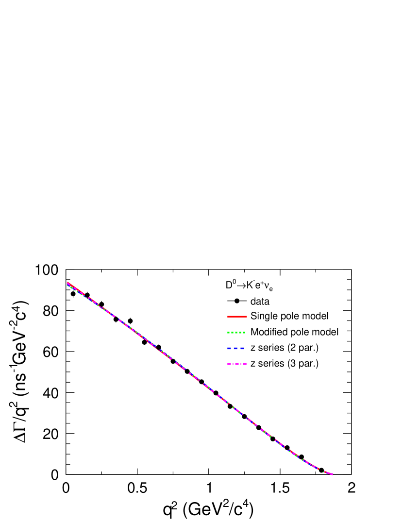
Figure 6: Differential decay rates for $D^{0}\rightarrow K^{-}e^{+}\nu_{e}$ as function of $q^{2}$. The dots with error bars show the data and the lines give the best fits to the data with different form-factor parameterizations.

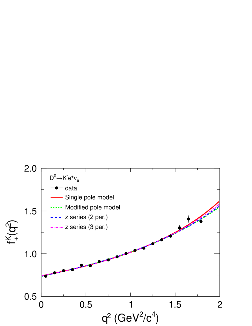
Figure 7: Projections on $f_{+}^{K}(q^{2})$ for $D^{0}\to K^{-}e^{+}\nu_{e}$.

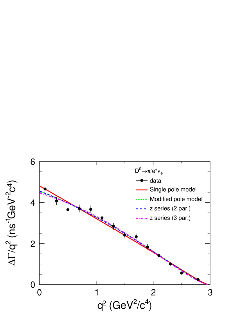
Figure 8: Differential decay rates for $D^{0}\rightarrow\pi^{-}e^{+}\nu_{e}$ as function of $q^{2}$. The dots with error bars show the data and the lines give the best fits to the data with different form-factor parameterizations.

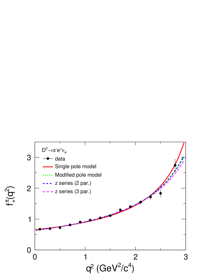
Figure 9: Projections on $f_{+}^{\pi}(q^{2})$ for $D^{0}\to\pi^{-}e^{+}\nu_{e}$.

Figures 9 and 9 show the projections of fits onto $f_{+}(q^{2})$ for the $D^{0}\to K^{-}e^{+}\nu_{e}$ and $D^{0}\to\pi^{-}e^{+}\nu_{e}$ decays, respectively. In these two figures, the dots with error bars show the measured values of the form factors, $f_{+}^{K(\pi)}(q^{2})$, which are obtained with

$$f_{+}^{K(\pi)}(q^{2}_{i})=\sqrt{\frac{\Delta\Gamma_{i}}{\Delta q^{2}_{i}}\frac{24\pi^{3}}{G_{F}^{2}{p^{\prime}}^{3}_{K(\pi)}|V_{cs(d)}|^{2}}}$$ (VI.21)

in which

$${p^{\prime}}^{3}_{K(\pi)}(i)=\frac{\int_{q^{2}_{{\rm min}(i)}}^{q^{2}_{{\rm max}(i)}}p^{3}_{K(\pi)}|f_{+}^{K(\pi)}(q^{2})|^{2}dq^{2}}{|f_{+}^{K(\pi)}(q^{2}_{i})|^{2}(q^{2}_{{\rm max}(i)}-q^{2}_{{\rm min}(i)})},$$ (VI.22)

where $|V_{cs}|=0.97343\pm 0.00015$ and $|V_{cd}|=0.22522\pm 0.00061$ are taken from the SM constraint fit pdg2014 . In the calculation of ${p^{\prime}}^{3}_{K(\pi)}(i)$, $f_{+}^{K(\pi)}(q^{2})$ and $f_{+}^{K(\pi)}(q^{2}_{i})$ are computed using the two parameter series parameterization with the measured parameters.

Table 13: Summary of results of form factor fits to the data.

Single pole model
Decay mode	$f_{+}^{K(\pi)}(0)|V_{cs(d)}|$	$M_{\rm pole}$ (GeV$/c^{2}$)		$\chi^{2}/$d.o.f.
$D^{0}\to K^{-}e^{+}\nu_{e}$	$0.7209\pm 0.0022\pm 0.0035$	$1.921\pm 0.010\pm 0.007$		$18.8/16$
$D^{0}\to\pi^{-}e^{+}\nu_{e}$	$0.1475\pm 0.0014\pm 0.0005$	$1.911\pm 0.012\pm 0.004$		$20.0/12$
Modified pole model
Decay mode	$f_{+}^{K(\pi)}(0)|V_{cs(d)}|$	$\alpha$		$\chi^{2}/$d.o.f.
$D^{0}\to K^{-}e^{+}\nu_{e}$	$0.7163\pm 0.0024\pm 0.0034$	$0.309\pm 0.020\pm 0.013$		$20.2/16$
$D^{0}\to\pi^{-}e^{+}\nu_{e}$	$0.1437\pm 0.0017\pm 0.0008$	$0.279\pm 0.035\pm 0.011$		$12.6/12$
Two-parameter series expansion
Decay mode	$f_{+}^{K(\pi)}(0)|V_{cs(d)}|$	$r_{1}$		$\chi^{2}/$d.o.f.
$D^{0}\to K^{-}e^{+}\nu_{e}$	$0.7172\pm 0.0025\pm 0.0035$	$-2.2286\pm 0.0864\pm 0.0573$		$19.6/16$
$D^{0}\to\pi^{-}e^{+}\nu_{e}$	$0.1435\pm 0.0018\pm 0.0009$	$-2.0365\pm 0.0807\pm 0.0257$		$12.8/12$
Three-parameter series expansion
Decay mode	$f_{+}^{K(\pi)}(0)|V_{cs(d)}|$	$r_{1}$	$r_{2}$	$\chi^{2}/$d.o.f.
$D^{0}\to K^{-}e^{+}\nu_{e}$	$0.7195\pm 0.0035\pm 0.0041$	$-2.3338\pm 0.1587\pm 0.0804$	$3.4188\pm 3.9090\pm 2.4098$	$19.1/15$
$D^{0}\to\pi^{-}e^{+}\nu_{e}$	$0.1420\pm 0.0024\pm 0.0010$	$-1.8432\pm 0.2212\pm 0.0690$	$-1.3874\pm 1.4615\pm 0.4680$	$11.9/11$

VI.5 Comparison of form-factor parameters in different parameterizations

For the single pole model, the fits give

$$M_{\rm pole}^{D\rightarrow K}=(1.921\pm 0.010\pm 0.007)~{}{\rm GeV}/c^{2},$$ (VI.23)

and

$$M_{\rm pole}^{D\rightarrow\pi}=(1.911\pm 0.012\pm 0.004)~{}{\rm GeV}/c^{2}$$ (VI.24)

for $D^{0}\rightarrow K^{-}e^{+}\nu_{e}$ and $D^{0}\rightarrow\pi^{-}e^{+}\nu_{e}$ decays, respectively. The agreement between the extracted values of pole mass and the expected values ($M_{D^{*+}_{(s)}}$) is extremely poor. For comparison, Table 14 lists the values of the pole mass $M_{\rm pole}^{D\rightarrow K}$ and $M_{\rm pole}^{D\rightarrow\pi}$ measured in this analysis and those previously measured at other experiments.

Table 14: Comparison of measurements of the pole masses $M^{D\rightarrow K}_{\rm pole}$ and $M^{D\rightarrow\pi}_{\rm pole}$.

Experiment	$M^{D\rightarrow K}_{\rm pole}$ (GeV$/c^{2}$)	$M^{D\rightarrow\pi}_{\rm pole}$ (GeV$/c^{2}$)
Mark III mark-iii	$1.80^{+0.50}_{-0.20}\pm 0.25$
E691 e691	$2.10^{+0.40}_{-0.20}\pm 0.20$
CLEO cleo_prd_44_3394	$2.10^{+0.40}_{-0.20}\pm 0.25$
CLEOII cleo_ii_plb_317_647	$2.00\pm 0.12\pm 0.18$
E687 (Tag) e687	$1.97^{+0.43}_{-0.22}\pm 0.07$
E687 (Incl) e687	$1.87^{+0.11}_{-0.08}\pm 0.07$
CLEO-II cleo_prl_94_011802	$1.89\pm 0.05^{+0.04}_{-0.03}$	$1.86^{+0.10}_{-0.06}\pm 0.05$
FOCUS focus_plb_607_233	$1.93\pm 0.05\pm 0.03$	$1.91^{+0.15}_{-0.30}\pm 0.07$
Belle bell_Phys_RevLett_97_p061804_y2006	$1.82\pm 0.04\pm 0.03$	$1.97\pm 0.08\pm 0.04$
BABAR BaBar_Phys_Rev_D76_p052005_y2007 ; BaBar_D0topienu	$1.884\pm 0.012\pm 0.015$	$1.906\pm 0.029\pm 0.023$
CLEO-c cleo-c_Phys_Rev_D79_052010_y2009	$1.97\pm 0.03\pm 0.01$	$1.95\pm 0.04\pm 0.02$
CLEO-c cleo-c_Phys_Rev_D77_112005_y2008	$1.97\pm 0.03\pm 0.01$	$1.87\pm 0.03\pm 0.01$
BESIII (This work)	$1.921\pm 0.010\pm 0.007$	$1.911\pm 0.012\pm 0.004$

With the modified pole model, the fits give

$$\alpha^{D\rightarrow K}=0.310\pm 0.020\pm 0.013,$$ (VI.25)

and

$$\alpha^{D\rightarrow\pi}=0.279\pm 0.035\pm 0.011$$ (VI.26)

for $D^{0}\rightarrow K^{-}e^{+}\nu_{e}$ and $D^{0}\rightarrow\pi^{-}e^{+}\nu_{e}$ decays, respectively. In the modified pole model (BK parameterization) for the form factors, $\alpha^{D\rightarrow K}_{\rm BK}$ is expected to be $\sim 1.75$ and $\alpha^{D\rightarrow\pi}_{\rm BK}$ is expected to be $\sim 1.34$ cleo-c_Phys_Rev_D79_052010_y2009 . Our measured values of $\alpha^{D\rightarrow K}$ and $\alpha^{D\rightarrow\pi}$ significantly deviate from the values required by the modified pole model. Table 15 presents a comparison of our measurements of these two parameters with those previously measured at other experiments and the expected values from the Lattice QCD calculations.

Table 15: Comparison of measurements of the shape parameters $\alpha^{D\rightarrow K}$ and $\alpha^{D\rightarrow\pi}$ in the modified pole model.

Theory/Experiment	$\alpha^{D\rightarrow K}$	$\alpha^{D\rightarrow\pi}$
LQCD lqcd_prl_94_011601	$0.50\pm 0.04\pm 0.07$	$0.44\pm 0.04\pm 0.07$
LCSR lcsr_nucl40_527	$0.07^{+0.15}_{-0.07}$	$0.11^{+0.11}_{-0.07}$
FOCUS focus_plb_607_233	$0.28\pm 0.08\pm 0.07$
Belle bell_Phys_RevLett_97_p061804_y2006	$0.52\pm 0.08\pm 0.06$	$0.10\pm 0.21\pm 0.10$
CLEO-c($281~{}\rm pb^{-1}$)(tagged) cleo-c_Phys_Rev_D79_052010_y2009	$0.21\pm 0.05\pm 0.02$	$0.16\pm 0.10\pm 0.05$
CLEO-c($281~{}\rm pb^{-1}$)(untagged) cleo-c_Phys_Rev_D77_112005_y2008	$0.21\pm 0.05\pm 0.03$	$0.37\pm 0.08\pm 0.03$
CLEO-c($818~{}\rm pb^{-1}$) cleo-c_Phys_Rev_D80_032005_y2009	$0.30\pm 0.03\pm 0.01$	$0.21\pm 0.07\pm 0.02$
BABAR BaBar_Phys_Rev_D76_p052005_y2007 ; BaBar_D0topienu	$0.377\pm 0.023\pm 0.029$	$0.268\pm 0.074\pm 0.059$
BESIII (This work)	$0.309\pm 0.020\pm 0.013$	$0.279\pm 0.035\pm 0.011$

VI.6 Comparison of the measured $f_{+}^{K(\pi)}(q^{2})$ with LQCD predictions

Figures 10 (a) and (b) show comparisons between our measured form factors and those calculated in LQCD lqcd_prl_94_011601 for $D^{0}\to K^{-}e^{+}\nu_{e}$ and $D^{0}\to\pi^{-}e^{+}\nu_{e}$ semileptonic decays, respectively. From these two figures we find that, although our measured values of the form factors $f^{K}_{+}(q^{2})$ and $f^{\pi}_{+}(q^{2})$ are consistent within uncertainties with the LQCD predictions, our measured values of the form factors significantly deviate from the most probable values calculated in LQCD in the regions above 0.75 GeV${}^{2}/c^{4}$ and 1.5 GeV${}^{2}/c^{4}$ for $D^{0}\to K^{-}e^{+}\nu_{e}$ and $D^{0}\to\pi^{-}e^{+}\nu_{e}$ decays, respectively. The precision of the measured $f_{+}^{K}(q^{2})$ and $f_{+}^{\pi}(q^{2})$ is much higher than that of the LQCD calculations.

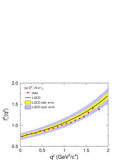
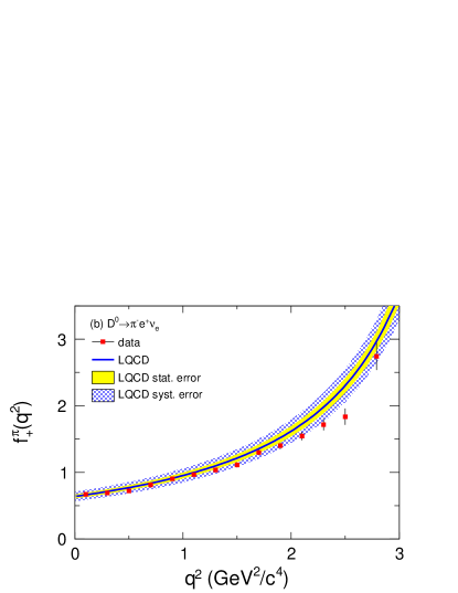
Figure 10: Comparisons of the measured form factors (squares with error bars) with the LQCD calculations lqcd_prl_94_011601 (solid lines present the central values, bands present the LQCD uncertainties).

VI.7 Comparison of measurements of $f^{K}_{+}(0)$ and $f^{\pi}_{+}(0)$

Using the measured $f_{+}^{K(\pi)}(0)|V_{cs(d)}|$ from the two-parameter series expansion fits, we obtain

$$\frac{f_{+}^{\pi}(0)|V_{cd}|}{f_{+}^{K}(0)|V_{cs}|}=0.2001\pm 0.0026\pm 0.0016,$$ (VI.27)

where the first error is statistical and second systematic. With the values of $|V_{cs(d)}|$ from the SM constraint fit pdg2014 , we find

$$\frac{f_{+}^{\pi}(0)}{f_{+}^{K}(0)}=0.8649\pm 0.0112\pm 0.0073,$$ (VI.28)

where the first error is statistical and second systematic. This measured ratio, ${f_{+}^{\pi}(0)}/{f_{+}^{K}(0)}=0.865\pm 0.013$, is in excellent agreement with the LCSR calculation of ${f_{+}^{\pi}(0)}/{f_{+}^{K}(0)}=0.84\pm 0.04$ LCSR_1 , but the precision is higher than the LCSR calculation by more than a factor of 3.

Using the $f_{+}^{K}(\pi)(0)|V_{cs(d)}|$ values from the two-parameter series expansion fits and taking the values of $|V_{cs(d)}|$ from the SM constraint fit pdg2014 as inputs, we obtain the form factors

$$f_{+}^{K}(0)=0.7368\pm 0.0026\pm 0.0036$$ (VI.29)

and

$$f_{+}^{\pi}(0)=0.6372\pm 0.0080\pm 0.0044,$$ (VI.30)

where the first errors are statistical and the second systematic.

Tables 16 and 17 show the comparisons of our measured form factors with those measured at other experiments, for which different form-factor parameterizations and values of $|V_{cs(d)}|$ have been used. Our measurements of these two form factors are consistent within errors with other measurements, but with a higher precision.

Table 16: Comparison of the form factor $f^{K}_{+}(0)$ measured at different experiments.

Experiment	$f^{K}_{+}(0)$	Form-factor parameterization
BES-II bes2_plb597_p39_2004	$0.78\pm 0.04\pm 0.03$	Single pole model
Belle bell_Phys_RevLett_97_p061804_y2006	$0.695\pm 0.007\pm 0.022$	Modified pole model
BABAR BaBar_Phys_Rev_D76_p052005_y2007	$0.727\pm 0.007\pm 0.005\pm 0.007$	Single pole model and modified pole model
CLEO-c cleo-c_Phys_Rev_D80_032005_y2009	$0.739\pm 0.007\pm 0.005\pm 0.000$	Three-parameter series expansion
BESIII (This work)	$0.7368\pm 0.0026\pm 0.0036$	Two-parameter series expansion

Table 17: Comparison of the form factor $f^{\pi}_{+}(0)$ measured at different experiments.

Experiment	$f^{\pi}_{+}(0)$	Form-factor parameterization
BES-II bes2_plb597_p39_2004	$0.73\pm 0.14\pm 0.06$	Single pole model
Belle bell_Phys_RevLett_97_p061804_y2006	$0.624\pm 0.020\pm 0.003$	Modified pole model
CLEO-c cleo-c_Phys_Rev_D80_032005_y2009	$0.666\pm 0.019\pm 0.004\pm 0.003$	Three-parameter series expansion
BABAR BaBar_D0topienu	$0.610\pm 0.020\pm 0.005$	Three-parameter series expansion
BESIII (This work)	$0.6372\pm 0.0080\pm 0.0044$	Two-parameter series expansion

VII Extraction of $|V_{cs}|$ and $|V_{cd}|$

VII.1 Determination of $|V_{cs}|$ and $|V_{cd}|$

Using the values for $f_{+}^{K}(\pi)(0)|V_{cs(d)}|$ from the two-parameter $z$-series expansion fits and in conjunction with $f_{+}^{K}(0)=0.747\pm 0.011\pm 0.015$ LQCD_fK and $f_{+}^{\pi}(0)=0.666\pm 0.020\pm 0.021$ LQCD_fpi calculated in LQCD, we obtain

$$|V_{cs}|=0.9601\pm 0.0033\pm 0.0047\pm 0.0239$$ (VII.1)

and

$$|V_{cd}|=0.2155\pm 0.0027\pm 0.0014\pm 0.0094,$$ (VII.2)

where the first uncertainties are statistical, the second ones systematic, and the third ones are due to the theoretical uncertainties in the form factor calculations.

From the measured ratio of $\frac{f_{+}^{\pi}(0)|V_{cd}|}{f_{+}^{K}(0)|V_{cs}|}$ given in Eq.(VI.27) together with the LCSR calculation of $f_{+}^{\pi}(0)/f_{+}^{K}(0)=0.84\pm 0.04$ LCSR_1 , we determine

$$\frac{|V_{cd}|}{|V_{cs}|}=0.238\pm 0.004\pm 0.002\pm 0.011,$$ (VII.3)

where the first error is statistical, the second one systematic, and the third one is from LCSR normalization.

VII.2 Comparison of $|V_{cs}|$ and $|V_{cd}|$

Table 18 and Table 19 give comparisons of our measured $|V_{cs}|$ and $|V_{cd}|$ with those measured at other experiments. Our measurements of $|V_{cs}|$ and $|V_{cd}|$ are of higher precision than previous results from both $D$ meson decays and $W$ boson decays.

Table 18: Comparison of $|V_{cs}|$ measurements.

Experiment	$|V_{cs}|$	Note
PDG2014 pdg2014	$0.986\pm 0.016$	Using $D_{s}^{+}\rightarrow\ell^{+}\nu_{\ell}$, $D^{0}\rightarrow K^{-}\ell^{+}\nu_{\ell}$ and $D^{+}\to\bar{K}^{0}e^{+}\nu_{e}$
PDG2014 pdg2014	$1.008\pm 0.021$	Using $D^{+}_{s}\rightarrow\ell^{+}\nu_{\ell}$
PDG2014 pdg2014	$0.953\pm 0.008\pm 0.024$	Using $D^{0}\rightarrow K^{-}\ell^{+}\nu_{\ell}$ and $D^{+}\to\bar{K}^{0}e^{+}\nu_{e}$
PDG2014 pdg2014	$0.97343\pm 0.00015$	Global fit in the Standard Model
PDG2006 pdg2006	$0.94^{+0.32}_{-0.26}\pm 0.14$	Using $W$ boson decay
BES-II bes2_plb597_p39_2004	$1.00\pm 0.05\pm 0.11$	Using $D^{0}\rightarrow K^{-}e^{+}\nu_{e}$
CLEO-c cleo-c_Phys_Rev_D80_032005_y2009	$0.985\pm 0.009\pm 0.006\pm 0.103$	Using $D^{0}\rightarrow K^{-}e^{+}\nu_{e}$ and $D^{+}\to\bar{K}^{0}e^{+}\nu_{e}$
BESIII (This work)	$0.9601\pm 0.0033\pm 0.0047\pm 0.0239$	Using $D^{0}\rightarrow K^{-}e^{+}\nu_{e}$

Table 19: Comparison of $|V_{cd}|$ measurements.

Experiment	$|V_{cd}|$	Note
PDG2014 pdg2014	$0.225\pm 0.008$	Using $D^{0}\to\pi^{-}\ell^{+}\nu_{\ell}$, $D^{+}\to\pi^{0}e^{+}\nu_{e}$ and neutrino interactions
PDG2014 pdg2014	$0.220\pm 0.006\pm 0.010$	Using $D^{0}\to\pi^{-}\ell^{+}\nu_{\ell}$ and $D^{+}\to\pi^{0}e^{+}\nu_{e}$
PDG2014 pdg2014	$0.230\pm 0.011$	Using neutrino interactions
PDG2014 pdg2014	$0.22522\pm 0.00061$	Global fit in the Standard Model
CLEO-c cleo-c_Phys_Rev_D80_032005_y2009	$0.234\pm 0.007\pm 0.002\pm 0.025$	Using $D^{0}\rightarrow\pi^{-}e^{+}\nu_{e}$ and $D^{+}\to\pi^{0}e^{+}\nu_{e}$
BESIII RongG_Charm2012	$0.2210\pm 0.0058\pm 0.0047$	Using $D^{+}\rightarrow\mu^{+}\nu_{\mu}$
BABAR BaBar_D0topienu	$0.206\pm 0.007\pm 0.009$	Using $D^{0}\rightarrow\pi^{-}e^{+}\nu_{e}$
BESIII (This work)	$0.2155\pm 0.0027\pm 0.0014\pm 0.0094$	Using $D^{0}\rightarrow\pi^{-}e^{+}\nu_{e}$

Table 20 gives a comparison of our measured ${|V_{cd}|}/{|V_{cs}|}$ with the one measured by CLEO-c cleo-c_Phys_Rev_D80_032005_y2009 and the world average calculated with $|V_{cd}|$ and $|V_{cs}|$ given in PDG2014 pdg2014 . Our measurement of the ratio is in excellent agreement with the world average.

Table 20: Comparison of $|V_{cd}|/|V_{cs}|$ measurements.

Experiment	$|V_{cd}|/|V_{cs}|$	Note
PDG2014 pdg2014	$0.228\pm 0.009$	Using $|V_{cd}|=0.225\pm 0.008$ and $|V_{cs}|=0.986\pm 0.016$
CLEO-c cleo-c_Phys_Rev_D80_032005_y2009	$0.242\pm 0.011\pm 0.004\pm 0.012$	Using $D\rightarrow\pi e^{+}\nu_{e}$ and $D\rightarrow Ke^{+}\nu_{e}$
BESIII (This work)	$0.238\pm 0.004\pm 0.002\pm 0.011$	Using $D^{0}\rightarrow\pi^{-}e^{+}\nu_{e}$ and $D^{0}\rightarrow K^{-}e^{+}\nu_{e}$

VIII Summary

In summary, by analyzing about 2.92 fb^-1 data collected at 3.773 GeV with the BESIII detector operated at the BEPCII collider, the semileptonic decays of $D^{0}\rightarrow K^{-}e^{+}\nu_{e}$ and $D^{0}\rightarrow\pi^{-}e^{+}\nu_{e}$ have been studied. From a total of $2793317\pm 3684$ single $\bar{D}^{0}$ tags, $70727.0\pm 278.3$ $D^{0}\to K^{-}e^{+}\nu_{e}$ and $6297.1\pm 86.8$ $D^{0}\to\pi^{-}e^{+}\nu_{e}$ signal events are observed in the system recoiling against the single $\bar{D}^{0}$ tags. These yield the decay branching fractions

$$\mathcal{B}(D^{0}\to K^{-}e^{+}\nu_{e})=(3.505\pm 0.014\pm 0.033)\%$$

and

$$\mathcal{B}(D^{0}\to\pi^{-}e^{+}\nu_{e})=(0.295\pm 0.004\pm 0.003)\%.$$

Using these samples of $D^{0}\rightarrow K^{-}e^{+}\nu_{e}$ and $D^{0}\rightarrow\pi^{-}e^{+}\nu_{e}$ decays, we study the form factors as a function of the squared four-momentum transfer $q^{2}$ for these two decays. By fitting the partial decays rates, we obtain the parameter values for several different form-factor functions. For the physical interpretation of the shape parameters in the single pole and modified pole models, the values of the parameters obtained from our fits significantly deviate from those expected by these models. This means that the data do not support the physical interpretation of the shape parameter in those models. We choose the values of $f_{+}^{K}(0)|V_{cs}|$ and $f_{+}^{\pi}(0)|V_{cd}|$ obtained with the two-parameter series expansion as our main result. In this case, we obtain the form factors

$$f^{K}_{+}(0)=0.7368\pm 0.0026\pm 0.0036$$

and

$$f^{\pi}_{+}(0)=0.6372\pm 0.0080\pm 0.0044.$$

Furthermore, using the form factors calculated in recent LQCD calculations LQCD_fK ; LQCD_fpi , we obtain the CKM matrix elements

$$|V_{cs}|=0.9601\pm 0.0033\pm 0.0047\pm 0.0239$$

and

$$|V_{cd}|=0.2155\pm 0.0027\pm 0.0014\pm 0.0094,$$

where the errors are dominated by the theoretical uncertainties in the form factor calculations. Our measurement of the product $f_{+}^{K}(0)|V_{cs}|=0.7172\pm 0.0025\pm 0.0035$ ($f_{+}^{\pi}(0)|V_{cd}|=0.1435\pm 0.0018\pm 0.0009$) is the most precise to date and would give more precise value of $|V_{cs}|$ ($|V_{cd}|$) with its precision increasing to $0.6\%$ ($1.4\%$) when the uncertainty of the value of the related form factor calculated in LQCD can be ignored.

Our measurements of the branching fractions, the form-factor parameters and the shapes of the form factor $f_{+}^{K(\pi)}(q^{2})$ as a function of $q^{2}$ for $D^{0}\to K^{-}e^{+}\nu_{e}$ and $D^{0}\to\pi^{-}e^{+}\nu_{e}$ decays are all the most precise to date. These precise measurements of $f_{+}^{K}(q^{2})$, $f_{+}^{\pi}(q^{2})$, $f_{+}^{K}(0)$, $f_{+}^{\pi}(0)$ and $f_{+}^{\pi}(0)/f_{+}^{K}(0)$ are in good agreement with the LQCD calculations of the form factors and the LCSR calculations of the ratio of the form factors, but have higher precision than those calculated in theories based on QCD, and therefore will allow incisive tests of any future theoretical calculations.

References

(1)
N. Cabibbo, Phys. Rev. Lett. 10, 531 (1963).
(2)
M. Kobayashi and T. Maskawa, Prog. Theor. Phys. 49, 652 (1973).
(3)
G. Rong, Chin. Phys. C 34(6), 788 (2010);
G. Rong, Y. Fang, H.L. Ma, J.Y. Zhao, Phys. Lett. B 743, 315 (2015).
(4)
M. Ablikim et al. (BESIII Collaboration), Nucl. Instrum. Methods Phys. Res. Sect. A 614, 345 (2010).
(5)
C. Zhang for BEPC & BEPCII Teams, Performance of the BEPC and progress of
the BEPCII, in: Proceedings of APAC, 2004, p. 15-19, Gyeongju, Korea.
(6)
K. A. Olive et al. (Particle Data Group), Chin. Phys. C 38, 090001 (2014).
(7)
T. Becher and R.J. Hill, Phys. Lett. B 633, 61 (2006).
(8) J.G. Körner and G.A. Schuler,
Z. Phys. C 38, 511 (1988);
J.G. Körner and G.A. Schuler,
Phys. Lett. B 226, 185 (1989);
J.G. Körner and G.A. Schuler,
Z. Phys. C 46, 93 (1990);
J.G. Körner, K. Schilcher, M. Wirbel and Y.L. Wu,
Z. Phys. C 48, 663 (1990).
(9) M. Wirbel, B. Stech and M. Bauer,
Z. Phys. C 29, 637 (1985);
M. Bauer and M. Wirbel,
Z. Phys. C 42, 671 (1989).
(10)
D. Becirevic and A.B. Kaidalov, Phys. Lett. B 478, 417 (2000).
(11)
C.G. Boyd, B. Grinstein, and R.F. Lebed, Nucl. Phys. B 461, 493 (1996).
(12)
N. Isgur and M.B. Wise, Phys. Lett. B 232, 113 (1989);
237 527 (1990); E. Eichten and B. Hill, Phys. Lett. B 234, 511 (1990);
H. Georgi, Phys. Lett. B 240, 447 (1990).
(13)
A. Khodjamirian et al. , Phys. Rev. D 62, 114002 (2000).
(14)
C. Aubin et al. (Fermilab Lattice Collaboration, MILC Collaboration, and HPQCD Collaboration), Phys. Rev. Lett. 94, 011601 (2005).
(15)
J.Z. Bai et al. (BES Collaboration), Nucl. Instrum. Methods Phys. Res. Sect. A 458, 627 (2001); 344, 319 (1994).
(16)
M.H. Ye and Z.P. Zheng, Int. J. Mod. Phys. A 2, 1707 (1987);
(17)
S. Agostinelli et al. (GEANT4 Collaboration), Nucl. Instrum.
Methods Phys. Res., Sect. A 506, 250 (2003).
(18)
Z. Y. Deng et al., Chinese Phys. C 30, 371 (2006).
(19)
S. Jadach, B. F. L. Ward, and Z. Was, Comput. Phys. Commun. 130, 260 (2000).
(20)
D. J. Lange, Nucl. Instrum. Meth. A 462, 152 (2001);
R.-G. Ping, Chin. Phys. C 32, 599 (2008).
(21)
M. Ablikim et al. (BES Collaboration), Phys. Lett. B 597, 39 (2004).
(22)
M. Ablikim et al. (BES Collaboration), Phys. Lett. B 603, 130 (2004); 608, 24 (2005); 610, 183 (2005).
(23)
H. Albrecht et al. (ARGUS Collaboration), Phys. Lett. B 241, 278 (1990).
(24)
J.Y. Ge et al. (CLEO Collaboration), Phys. Rev. D 79, 052010 (2009).
(25)
J. Adler et al (Mark III Collaboration), Phys. Rev. Lett. 62, 1821 (1989).
(26)
F. Butler et al. (CLEO Collaboration), Phys. Rev. D 52, 2656 (1995).
(27)
T.E. Coan et al. (CLEO Collaboration), Phys. Rev. Lett. 95, 181802 (2005).
(28)
D. Besson et al. (CLEO Collaboration), Phys. Rev. D 80, 032005 (2009).
(29)
L. Widhalm et al. (Belle Collaboration), Phys. Rev. Lett. 97, 061804 (2006).
(30)
B. Aubert et al. (BABAR Collaboration), Phys. Rev. D 76, 052005 (2007).
(31)
J.P. Lees et al. (BABAR Collaboration), Phys. Rev. D 91, 052022 (2015).
(32)
A. Abada, Nucl. Phys. B 619, 565 (2001).
(33)
P. Ball, V. M. Braun, and H. G. Dosch, Phys, Rev. D 44, 3567 (1991).
(34)
W. Y. Wang, Y. L. Wu, and M. Zhong, Phys, Rev. D 67, 014024 (2003).
(35)
M. Lefebvre, R.K. Keeler, R. Sobie, and J. White, Nucl. Instrum. Methods Phys. Res., Sect. A 451, 520 (2000).
(36)
J.C. Anjos et al. (E691 Collaboration), Phys. Rev. Lett. 62, 1587 (1989).
(37)
G. Crawford et al. (CLEO Collaboration), Phys, Rev. D 44, 3394 (1991).
(38)
A. Bean et al. (CLEO Collaboration), Phys. Lett. B 317, 647 (1993).
(39)
P.L. Frabetti et al. (E687 Collaboration), Phys. Lett. B 364, 127 (1995).
(40)
G.S. Huang et al. (CLEO Collaboration), Phys. Rev. Lett. 94, 011802 (2005).
(41)
J.M. Link et al. (FOCUS Collaboration), Phys. Lett. B 607, 233 (2005).
(42)
T.M. Aliev, V.L. Eletsky, and Y.I. Kogan, Sov. J. Nucl. Phys. 40, 527 (1984).
(43)
S. Dobbs et al. (CLEO Collaboration), Phys. Rev. D 77, 112005 (2008).
(44)
P. Ball, Phys. Lett. B 641, 50 (2006).
(45)
H. Na et al. (HPQCD Collaboration), Phys. Rev. D 82, 114506 (2010).
(46)
H. Na et al. (HPQCD Collaboration), Phys. Rev. D 84, 114505 (2011).
(47)
W.M. Yao et al. (Particle Data Group), J. Phys. G 33, 1 (2006).
(48) M. Ablikim et al. (BESIII Collaboration), Phys. Rev. D 89, 051104(R) (2014).