Model selection in logistic regression

Abstract.

This paper is devoted to model selection in logistic regression. We extend the model selection principle introduced by Birgé and Massart birge2001gaussian to logistic regression model. This selection is done by using penalized maximum likelihood criteria. We propose in this context a completely data-driven criteria based on the slope heuristics. We prove non asymptotic oracle inequalities for selected estimators. Theoretical results are illustrated through simulation studies.

Keywords: logistic regression, model selection, projection.

AMS 2000 MSC: Primary 62J02, 62F12, Secondary 62G05, 62G20.

1. Introduction

Consider the following generalization of the logistic regression model : let $(Y_{1},x_{1}),\cdots,(Y_{n},x_{n})$, be a sample of size $n$ such that $(Y_{i},x_{i})\in\{0,1\}\times\mathcal{X}$ and

$$\mathbb{E}_{f_{0}}(Y_{i})=\pi_{f_{0}}(x_{i})=\frac{\exp{f_{0}(x_{i})}}{1+\exp{f_{0}(x_{i})}},$$

where $f_{0}$ is an unknown function to be estimated and the design points $x_{1},...,x_{n}$ are deterministic. This model can be viewed as a nonparametric version of the ”classical” logistic model which relies on the assumption that $x_{i}\in\mathbb{R}^{d}$, and that there exists $\beta_{0}\in\mathbb{R}^{d}$ such that $f_{0}(x_{i})=\beta_{0}^{\top}x_{i}.$

Logistic regression is a widely used model for predicting the outcome of binary dependent variable. For example logistic model can be used in medical study to predict the probability that a patient has a given disease (e.g. cancer), using observed characteristics (explanatory variables) of the patient such as weight, age, patient’s gender etc. However in the presence of numerous explanatory variables with potential influence, one would like to use only a few number of variables, for the sake of interpretability or to avoid overfitting. But it is not always obvious to choose the adequate variables. This is the well-known problem of variables selection or model selection.

In this paper, the unknown function $f_{0}$ is not specified and not necessarily linear. Our aim is to estimate $f_{0}$ by a linear combination of given functions, often called dictionary. The dictionary can be a basis of functions, for instance spline or polynomial basis.

A nonparametric version of the classical logistic model has already been considered by Hastie non_par_logist, where a nonparametric estimator of $f_{0}$ is proposed using local maximum likelihood. The problem of nonparametric estimation in additive regression model is well known and deeply studied. But in logistic regression model it is less studied. One can cite for instance Lu Lu2006, Vexler Vexler2006, Fan et al. Fanetal1998, Farmen Farmen1996, Raghavan Raghavan1993, and Cox Cox1990.

Recently few papers deal with model selection or nonparametric estimation in logistic regression using $\ell_{1}$ penalized contrast Bunea bunea2008honest, Bach bach10, van de Geer van2008, Kwemou kwemou. Among them, some establish non asymptotic oracle inequalities that hold even in high dimensional setting. When the dimension of $\mathcal{X}$ is high, that is greater than dozen, such $\ell_{1}$ penalized contrast estimators are known to provide reasonably good results. When the dimension of $\mathcal{X}$ is small, it is often better to choose different penalty functions. One classical penalty function is what we call $\ell_{0}$ penalization. Such penalty functions, built as increasing function of the dimension of $\mathcal{X}$, usually refers to model selection. The last decades have witnessed a growing interest in the model selection problem since the seminal works of Akaike akaike1973, Schwarz schwarz1978. In additive regression one can cite among the others Baraud baraud2000model, Birgé and Massart birge2001gaussian, Yang yang1999, in density estimation Birgé birge2014model, Castellan castellan2003density and in segmentation problem Lebarbier lebarbier, Durot et al. DurotLebarbierTocquet, and Braun et al. braun. All the previously cited papers use $\ell_{0}$ penalized contrast to perform model selection. But model selection procedures based on penalized maximum likelihood estimators in logistic regression are less studied in the literature.

In this paper we focus on model selection using $\ell_{0}$ penalized contrast for logistic regression model and in this context we state non asymptotic oracle inequalities. More precisely, given some collection functions, we consider estimators of $f_{0}$ built as linear combination of the functions. The point that the true function is not supposed to be linear combination of those functions, but we expect that the spaces of linear combination of those functions would provide suitable approximation spaces. Thus, to this collection of functions, we associate a collection of estimators of $f_{0}$. Our aim is to propose a data driven procedure, based on penalized criterion, which will be able to choose the ”best” estimator among the collection of estimators, using $\ell_{0}$ penalty functions.

The collection of estimators is built using minimisation of the opposite of logarithm likelihood. The properties of estimators are described in term of Kullback-Leibler divergence and the empirical $L_{2}$ norm. Our results can be splitted into two parts.

First, in a general model selection framework, with general collection of functions we provide a completely data driven procedure that automatically selects the best model among the collection. We state non asymptotic oracle inequalities for Kullback-Leibler divergence and the empirical $L_{2}$ norm between the selected estimator and the true function $f_{0}$. The estimation procedure relies on the building of a suitable penalty function, suitable in the sense that it performs best risks and suitable in the sense that it does not depend on the unknown smoothness parameters of the true function $f_{0}$. But, the penalty function depends on a bound related to target function $f_{0}$. This can be seen as the price to pay for the generality. It comes from needed links between Kullback-Leibler divergence and empirical $L_{2}$ norm.

Second, we consider the specific case of collection of piecewise functions which provide estimator of type regressogram. In this case, we exhibit a completely data driven penalty, free from $f_{0}$. The model selection procedure based on this penalty provides an adaptive estimator and state a non asymptotic oracle inequality for Hellinger distance and the empirical $L_{2}$ norm between the selected estimator and the true function $f_{0}$. In the case of piecewise constant functions basis, the connection between Kullback-Leibler divergence and the empirical $L_{2}$ norm are obtained without bound on the true function $f_{0}$. This last result is of great interest for example in segmentation study, where the target function is piecewise constant or can be well approximated by piecewise constant functions.

Those theoretical results are illustrated through simulation studies. In particular we show that our model selection procedure (with the suitable penalty) have good non asymptotic properties as compared to usual known criteria such as AIC and BIC. A great attention has been made on the practical calibration of the penalty function. This practical calibration is mainly based on the ideas of what is usually referred as slope heuristic as proposed in Birgé and Massart birge2007 and developed in Arlot and Massart arlot2009.

The paper is organized as follow. In Section 2 we set our framework and describe our estimation procedure. In Section 3 we define the model selection procedure and state the oracle inequalities in the general framework. Section 4 is devoted to regressogram selection, in this section, we establish a bound of the Hellinger risk between the selected model and the target function. The simulation study is reported in Section 5. The proofs of the results are postponed to Section 6 and  7.

2. Model and framework

Let $(Y_{1},x_{1}),\cdots,(Y_{n},x_{n})$, be a sample of size $n$ such that $(Y_{i},x_{i})\in\{0,1\}\times\mathcal{X}$. Throughout the paper, we consider a fixed design setting i.e. $x_{1},\dots,x_{n}$ are considered as deterministic. In this setting, consider the extension of the ”classical” logistic regression model (2.1) where we aim at estimating the unknown function $f_{0}$ in

(2.1) $$\mathbb{E}_{f_{0}}(Y_{i})=\pi_{f_{0}}(x_{i})=\frac{\exp{f_{0}(x_{i})}}{1+\exp{f_{0}(x_{i})}}.$$

We propose to estimate the unknown function $f_{0}$ by model selection. This model selection is performed using penalized maximum likelihood estimators. In the following we denote by $\mathbb{P}_{f_{0}}(x_{1})$ the distribution of $Y_{1}$ and by $\mathbb{P}^{(n)}_{f_{0}}(x_{1},\cdots,x_{n})$ the distribution of $(Y_{1},\dots,Y_{n})$ under Model (2.1). Since the variables $Y_{i}$’s are independent random variables,

$$\mathbb{P}^{(n)}_{f_{0}}(x_{1},\cdots,x_{n})=\Pi_{i=1}^{n}\mathbb{P}_{f_{0}}(x_{i})=\prod_{i=1}^{n}\pi_{f_{0}}(x_{i})^{Y_{i}}(1-\pi_{f_{0}}(x_{i}))^{1-Y_{i}}.$$

It follows that for a function $f$ mapping $\mathcal{X}$ into $\mathbb{R}$, the likelihood is defined as:

$$L_{n}(f)=\mathbb{P}^{(n)}_{f}(x_{1},\cdots,x_{n})=\prod_{i=1}^{n}\pi_{f}(x_{i})^{Y_{i}}(1-\pi_{f}(x_{i}))^{1-Y_{i}},$$

where

(2.2) $$\pi_{f}(x_{i})=\frac{\exp{(f(x_{i}))}}{1+\exp({f}(x_{i}))}.$$

We choose the opposite of the log-likelihood as the estimation criterion that is

(2.3) $$\gamma_{n}(f)=-\frac{1}{n}\log(L_{n}(f))=\frac{1}{n}\sum_{i=1}^{n}\Big{\{}\log(1+e^{f(x_{i})})-Y_{i}f(x_{i})\Big{\}}.$$

Associated to this estimation criterion we consider the Kullback-Leibler information divergence $\mathcal{K}(\mathbb{P}_{f_{0}}^{(n)},\mathbb{P}_{f}^{(n)})$ defined as

$$\mathcal{K}(\mathbb{P}_{f_{0}}^{(n)},\mathbb{P}_{f}^{(n)})=\frac{1}{n}\int\log\left(\frac{\mathbb{P}_{f_{0}}^{(n)}}{\mathbb{P}_{f}^{(n)}}\right)d\mathbb{P}_{f_{0}}^{(n)}.$$

The loss function is the excess risk, defined as

(2.4) $$\mathcal{E}(f):=\gamma(f)-\gamma(f_{0})\mbox{ where, for any }f,\quad\gamma(f)=\mathbb{E}_{f_{0}}[\gamma_{n}(f)].~{}~{}~{}~{}~{}$$

Easy calculations show that the excess risk is linked to the Kullback-Leibler information divergence through the relation

$$\mathcal{E}(f)=\gamma(f)-\gamma(f_{0})=\mathcal{K}(\mathbb{P}_{f_{0}}^{(n)},\mathbb{P}_{f}^{(n)}).$$

It follows that, $f_{0}$ minimizes the excess risk, that is

$$f_{0}=\arg\min_{f}\gamma(f).$$

As usual, one can not estimate $f_{0}$ by the minimizer of $\gamma_{n}(f)$ over any functions space, since it is infinite. The usual way is to minimize $\gamma_{n}(f)$ over a finite dimensional collections of models, associated to a finite dictionary of functions $\phi_{j}:\mathcal{X}\rightarrow\mathbb{R}$

$$\mathcal{D}=\{\phi_{1},\dots,\phi_{M}\}.$$

For the sake of simplicity we will suppose that $\mathcal{D}$ is a orthonormal basis of functions. Indeed, if $\mathcal{D}$ is not an orthonormal basis of functions, we can always find an orthonormal basis of functions $\mathcal{D^{\prime}}=\{\psi_{1},\dots,\psi_{M^{\prime}}\}$ such that

$$\langle\phi_{1},\dots,\phi_{M}\rangle=\langle\psi_{1},\dots,\psi_{M^{\prime}}\rangle.$$

Let $\mathcal{M}$ the set of all subsets $m\subset\{1,\dots,M\}$. For every $m\in\mathcal{M}$, we call $\mathcal{S}_{m}$ the model

(2.5) $$\mathcal{S}_{m}:=\Big{\{}f_{\beta}=\sum_{j\in m}\beta_{j}\phi_{j}\Big{\}}$$

and $D_{m}$ the dimension of the span of $\{\phi_{j},j\in m\}$. Given the countable collection of models $\{\mathcal{S}_{m}\}_{m\in\mathcal{M}}$, we define $\{\hat{f}_{m}\}_{m\in\mathcal{M}}$ the corresponding estimators, i.e. the estimators obtaining by minimizing $\gamma_{n}$ over each model $\mathcal{S}_{m}$. For each $m\in\mathcal{M}$, $\hat{f}_{m}$ is defined by

(2.6) $$\hat{f}_{m}=\arg\min_{t\in\mathcal{S}_{m}}\gamma_{n}(t).$$

Our aim is choose the ”best” estimator among this collection of estimators, in the sense that it minimizes the risk. In many cases, it is not easy to choose the ”best” model. Indeed, a model with small dimension tends to be efficient from estimation point of view whereas it could be far from the ”true” model. On the other side, a more complex model easily fits data but the estimates have poor predictive performance (overfitting). We thus expect that this best estimator mimics what is usually called the oracle defined as

(2.7) $$m^{*}=\arg\min_{m\in\mathcal{M}}\mathcal{K}(\mathbb{P}_{f_{0}}^{(n)},\mathbb{P}_{\hat{f}_{m}}^{(n)}).$$

Unfortunately, both, minimizing the risk and minimazing the kulback-leibler divergence, require the knowledge of the true (unknown) function $f_{0}$ to be estimated.

Our goal is to develop a data driven strategy based on data, that automatically selects the best estimator among the collection, this best estimator having a risk as close as possible to the oracle risk, that is the risk of $\hat{f}_{m^{*}}$. In this context, our strategy follows the lines of model selection as developed by Birgé and Massart birge2001gaussian. We also refer to the book Massart massart2007 for further details on model selection.

We use penalized maximum likelihood estimator for choosing some data-dependent $\hat{m}$ nearly as good as the ideal choice $m^{*}$. More precisely, the idea is to select $\hat{m}$ as a minimizer of the penalized criterion

(2.8) $$\hat{m}=\arg\min_{m\in\mathcal{M}}\left\{\gamma_{n}(\hat{f}_{m})+\mbox{pen}(m)\right\},$$

where $\mbox{pen}:\mathcal{M}\longrightarrow\mathbb{R}^{+}$ is a data driven penalty function. The estimation properties of $\hat{f}_{m}$ are evaluated by non asymptotic bounds of a risk associated to a suitable chosen loss function. The great challenge is choosing the penalty function such that the selected model $\hat{m}$ is nearly as good as the oracle $m{{}^{*}}$. This penalty term is classically based on the idea that

$$m^{*}=\arg\min_{m\in\mathcal{M}}\mathbb{E}_{f_{0}}\mathcal{K}(\mathbb{P}_{f_{0}}^{(n)},\mathbb{P}_{\hat{f}_{m}}^{(n)})=\arg\min_{m\in\mathcal{M}}\left[\mathbb{E}_{f_{0}}\mathcal{K}(\mathbb{P}_{f_{0}}^{(n)},\mathbb{P}_{f_{m}}^{(n)})+\mathbb{E}_{f_{0}}\mathcal{K}(\mathbb{P}_{f_{m}}^{(n)},\mathbb{P}_{\hat{f}_{m}}^{(n)})\right]$$

where $f_{m}$ is defined as

$$f_{m}=\arg\min_{t\in S_{m}}\gamma(t).$$

Our goal is to build a penalty function such that the selected model $\hat{m}$ fulfills an oracle inequality:

$$\mathcal{K}(\mathbb{P}_{f_{0}}^{(n)},\mathbb{P}_{\hat{f}_{\hat{m}}}^{(n)})\leq C_{n}\inf_{m\in\mathcal{M}}\mathcal{K}(\mathbb{P}_{f_{0}}^{(n)},\mathbb{P}_{\hat{f}_{m}}^{(n)})+R_{n}.$$

This inequality is expected to hold either in expectation or with high probability, where $C_{n}$ is as close to 1 as possible and $R_{n}$ is a remainder term negligible compared to $\mathcal{K}(\mathbb{P}_{f_{0}}^{(n)},\mathbb{P}_{\hat{f}_{m{*}}}^{(n)})$.

In the following we consider two separated case. First we consider general collection of models under boundedness assumption. Second we consider the specific case of regressogram collection.

3. Oracle inequality for general models collection under boundedness assumption

Consider model (2.1) and $(\mathcal{S}_{m})_{m\in\mathcal{M}}$ a collection of models defined by (2.5). Let $C_{0}>0$ and $\mathbb{L}_{\infty}(C_{0})=\Big{\{}f:\mathcal{X}\to\mathbb{R},~{}~{}\max_{1\leqslant i\leqslant n}|f(x_{i})|\leqslant C_{0}\Big{\}}$. For $m\in\mathcal{M}$, $\gamma_{n}$ given in (2.3), and $\gamma$ is given by (2.4), we define

(3.9) $$\hat{f}_{m}=\arg\min_{t\in\mathcal{S}_{m}\cap\mathbb{L}_{\infty}(C_{0})}\gamma_{n}(t)\mbox{ and }f_{m}=\arg\min_{t\in S_{m}\cap\mathbb{L}_{\infty}(C_{0})}\gamma(t).$$

The first step consists in studying the estimation properties of $\hat{f}_{m}$ for each $m$, as it is stated in the following proposition.

Proposition 3.1.

Let $C_{0}>0$ and $\mathcal{U}_{0}=e^{C_{0}}/(1+e^{C_{0}})^{2}$. For $m\in\mathcal{M}$, let $\hat{f}_{m}$ and $f_{m}$ as in (3.9). We have

$$\mathbb{E}_{f_{0}}[\mathcal{K}(\mathbb{P}_{f_{0}}^{(n)},\mathbb{P}_{\hat{f}_{m}}^{(n)})]\leqslant\mathcal{K}(\mathbb{P}_{f_{0}}^{(n)},\mathbb{P}_{f_{m}}^{(n)})+\frac{D_{m}}{2n\mathcal{U}_{0}^{2}}$$

This proposition says that the ”best” estimator amoung the collection $\{\hat{f}_{m}\}_{m\in\mathcal{M}}$, in the sense of the Kullback-Leibler risk, is the one which makes a balance between the bias and the complexity of the model. In the ideal situation where $f_{0}$ belongs to $\mathcal{S}_{m}$, we have that

$$\mathbb{E}_{f_{0}}[\mathcal{K}(\mathbb{P}_{f_{0}}^{(n)},\mathbb{P}_{\hat{f}_{m}}^{(n)})]\leqslant\frac{1}{\mathcal{U}_{0}^{2}}\frac{D_{m}}{2n}.$$

To derive the model selection procedure we need the following assumption :

($$\mathbf{A_{1}} \mbox{There exists a constant}~{}0<c_{1}<\infty~{}\mbox{such that }~{}\max_{1\leqslant i\leqslant n}|f_{0}(x_{i})|\leqslant c_{1}.~{}~{}~{}~{}~{}~{}~{}~{}~{}~{}~{}~{}~{}~{}~{}~{}~{}~{}~{}~{}~{}~{}~{}~{}~{}~{}~{}~{}~{}~{}~{}~{}~{}~{}~{}$$)

In the following theorem we propose a choice for the penalty function and we state non asymptotic risk bounds.

Theorem 3.1.

Given $C_{0}>0$, for $m\in\mathcal{M}$, let $\hat{f}_{m}$ and $f_{m}$ be defined as (3.9). Let us denote $\parallel f\parallel_{n}^{2}=n^{(-1)}\sum_{i=1}^{n}f^{2}(x_{i})$. Let $\{L_{m}\}_{m\in\mathcal{M}}$ some positive numbers satisfying

$$\Sigma=\sum_{m\in\mathcal{M}}\exp(-L_{m}D_{m})<\infty.$$

We define $\mbox{pen}:\mathcal{M}\rightarrow\mathbb{R}_{+}$ , such that, for $m\in\mathcal{M}$,

$$\mbox{pen}(m)\geqslant\lambda\frac{D_{m}}{n}\left(\frac{1}{2}+\sqrt{5L_{m}}\right)^{2},$$

where $\lambda$ is a positive constant depending on $c_{1}$. Under Assumption ($\mathbf{A_{1}}$) we have

$$\mathbb{E}_{f_{0}}[\mathcal{K}(\mathbb{P}_{f_{0}}^{(n)},\mathbb{P}_{\hat{f}_{\hat{m}}}^{(n)})]\leqslant C\inf_{m\in\mathcal{M}}\left\{\mathcal{K}(\mathbb{P}_{f_{0}}^{(n)},\mathbb{P}_{f_{m}}^{(n)})+\mbox{pen}(m)\right\}+C_{1}\frac{\Sigma}{n}$$

and

$$\mathbb{E}_{f_{0}}\parallel\hat{f}_{\hat{m}}-f_{0}\parallel_{n}^{2}\leqslant C^{\prime}\inf_{m\in\mathcal{M}}\left\{\parallel f_{0}-f_{m}\parallel_{n}^{2}+\mbox{pen}(m)\right\}+C_{1}^{\prime}\frac{\Sigma}{n}.$$

where $C,C^{\prime},C_{1},C_{1}^{\prime}$ are constants depending on $c_{1}$ and $C_{0}$.

This theorem provides oracle inequalities for $L_{2}-$norm and for K-L divergence between the selected model and the true function. Provided that penalty has been properly chosen, one can bound the $L_{2}-$norm and the K-L divergence between the selected model and the true function. The inequalities in Theorem 3.1 are non-asymptotic inequalities in the sense that the result is obtain for a fixed $n$. This theorem is very general and does not make specific assumption on the dictionary. However, the penalty function depends on some unknown constant $\lambda$ which depends on the bound of the true function $f_{0}$ through Condition (6.5). In practice this constant can be calibrated using ”slope heuristics” proposed in Birgé and Massart birge2007. In the following we will show how to obtain similar result with a penalty function not connected to the bound of the true unknown function $f_{0}$ in the regressogram case.

4. Regressogram functions

4.1. Collection of models

In this section we suppose (without loss of generality) that $f_{0}:[0,1]\to\mathbb{R}$. For the sake of simplicity, we use the notation $f_{0}(x_{i})=f_{0}(i)$ for every $i=1,\dots,n$. Hence $f_{0}$ is defined from $\{1,\dots,n\}$ to $\mathbb{R}$. Let $\mathcal{M}$ be a collection of partitions of intervals of $\mathcal{X}=\{1,\dots,n\}$. For any $m\in\mathcal{M}$ and $J\in m$, let ${{{1}}{\mathrm{I}}}_{J}$ denote the indicator function of $J$ and $S_{m}$ be the linear span of $\{{{{1}}{\mathrm{I}}}_{J},J\in m\}$. When all intervals have the same length, the partition is said regular, and is is irregular otherwise.

4.2. Collection of estimators: regressogram

For a fixed $m$, the minimizer $\hat{f}_{m}$ of the empirical contrast function $\gamma_{n}$, over $S_{m}$, is called the regressogram. That is, $f_{0}$ is estimated by $\hat{f}_{m}$ given by

(4.10) $$\hat{f}_{m}=\arg\min_{f\in S_{m}}\gamma_{n}(f).$$

where $\gamma_{n}$ is given by (2.3). Associated to $S_{m}$ we have

(4.11) $$f_{m}=\arg\min_{f\in S_{m}}\gamma(f)-\gamma(f_{0})=\arg\min_{f\in S_{m}}\mathcal{K}(\mathbb{P}_{f_{0}}^{(n)},\mathbb{P}_{f}^{(n)}).$$

In the specific case where $S_{m}$ is the set of piecewise constant functions on some partition $m$, $\hat{f}_{m}$ and ${f}_{m}$ are given by the following lemma.

Lemma 4.1.

For $m\in\mathcal{M}$ , let $f_{m}$ and $\hat{f}_{m}$ be defined by (4.11) and (4.10) respectively . Then, $f_{m}=\sum_{J\in m}\overline{f}_{m}^{(J)}{{{1}}{\mathrm{I}}}_{J}$ and $\hat{f}_{m}=\sum_{J\in m}\hat{f}_{m}^{(J)}{{{1}}{\mathrm{I}}}_{J}$ with

$$\overline{f}_{m}^{(J)}=\log\left(\frac{\sum_{i\in J}\pi_{f_{0}}(x_{i})}{|J|(1-\sum_{i\in J}\pi_{f_{0}}(x_{i})/|J|)}\right)\mbox{ and }\hat{f}_{m}^{(J)}=\log\left(\frac{\sum_{i\in J}Y_{i}}{|J|(1-\sum_{i\in J}Y_{i}/|J|)}\right).$$

Moreover, $\pi_{f_{m}}=\sum_{J\in m}\pi_{f_{m}}^{(J)}{{{1}}{\mathrm{I}}}_{J}$ and $\pi_{\hat{f}_{m}}=\sum_{J\in m}\pi_{\hat{f}_{m}}^{(J)}{{{1}}{\mathrm{I}}}_{J}$ with

$$\pi_{f_{m}}^{(J)}=\frac{1}{|J|}\sum_{i\in J}\pi_{f_{0}}(x_{i}),\mbox{ and }\pi_{\hat{f}_{m}}^{(J)}=\frac{1}{|J|}\sum_{i\in J}Y_{i}.$$

Consequently, $\pi_{f_{m}}=\arg\min_{\pi\in S_{m}}\parallel\pi-\pi_{f_{0}}\parallel^{2}_{n}$ is the usual projection of $\pi_{f_{0}}$ on to $S_{m}$.

4.3. First bounds on $\hat{f}_{m}$

Consider the following assumptions:

($$\mathbf{A_{2}} \mbox{ There exists a constant }\rho>0\mbox{ such that }\min_{i=1,\cdots,n}\pi_{f_{0}}(x_{i})\geq\rho~{}~{}\mbox{and}~{}~{}~{}\min_{i=1,\cdots,n}[1-\pi_{f_{0}}(x_{i})]\geq\rho.$$)

Proposition 4.1.

Consider Model (2.1) and let $\hat{f}_{m}$ be defined by (4.10) with $m$ such that for all $J\in m$, $|J|\geqslant\Gamma[\log(n)]^{2}$ for a positive constant $\Gamma$. Under Assumption ($\mathbf{A_{2}}$), for all $\delta>0$ and $a>1$, we have

$$\mathbb{E}_{f_{0}}[\mathcal{K}(\mathbb{P}_{f_{0}}^{(n)},\mathbb{P}_{\hat{f}_{m}}^{(n)})] \leqslant \mathcal{K}(\mathbb{P}_{f_{0}}^{(n)},\mathbb{P}_{f_{m}}^{(n)}))+\frac{(1+\delta)D_{m}}{(1-\delta)^{2}n}+\frac{\kappa(\Gamma,\rho,\delta)}{n^{a}}.$$

4.4. Adaptive estimation and oracle inequality

The following result provides an adaptive estimation of $f_{0}$ and a risk bound of the selected model.

Definition 4.1.

Let $\mathcal{M}$ be a collection of partitions of $\mathcal{X}=\{1,\dots,n\}$ constructed on the partition $m_{f}$ i.e. $m_{f}$ is a refinement of every $m\in\mathcal{M}.$

In other words, a partition $m$ belongs to $\mathcal{M}$ if any element of $m$ is the union of some elements of $m_{f}$. Thus $S_{m_{f}}$ contains every model of the collection $\{S_{m}\}_{m\in\mathcal{M}}$.

Theorem 4.1.

Consider Model (2.1) under Assumption ($\mathbf{A_{2}}$). Let $\{S_{m},m\in\mathcal{M}\}$ be a collection of models defined in Section 4.1 where $\mathcal{M}$ is a set of partitions constructed on the partition $m_{f}$ such that

(4.1) $$\mbox{for all}~{}~{}J\in m_{f},|J|\geq\Gamma\log^{2}(n),$$

where $\Gamma$ is a positive constant. Let $(L_{m})_{m\in\mathcal{M}}$ be some family of positive weights satisfying

(4.2) $$\Sigma=\sum_{m\in\mathcal{M}}\exp(-L_{m}D_{m})<+\infty.$$

Let $\mbox{pen}:\mathcal{M}\rightarrow\mathbb{R}_{+}$ satisfying for $m\in\mathcal{M}$, and for $\mu>1,$

$$\mbox{pen}(m)\geqslant\mu\frac{D_{m}}{n}\left(1+6L_{m}+8\sqrt{L_{m}}\right).$$

Let $\tilde{f}=\hat{f}_{\hat{m}}$ where

$$\hat{m}=\arg\min_{m\in\mathcal{M}}\left\{\gamma_{n}(\hat{f}_{m})+\mbox{pen}(m)\right\},$$

then, for $C_{\mu}=2\mu^{1/3}/(\mu^{1/3}-1)$, we have

(4.3) $$\mathbb{E}_{f_{0}}[h^{2}(\mathbb{P}^{(n)}_{f_{0}},\mathbb{P}^{(n)}_{\tilde{f}})]\leqslant C_{\mu}\inf_{m\in\mathcal{M}}\left\{\mathcal{K}(\mathbb{P}_{f_{0}}^{(n)},\mathbb{P}_{f_{m}}^{(n)})+\mbox{pen}(m)\right\}+\frac{C(\rho,\mu,\Gamma,\Sigma)}{n}.$$

This theorem provides a non asymptotic bound for the Hellinger risk between the selected model and the true one. On the opposite of Theorem 3.1, the penalty function does not depend on the bound of the true function. The selection procedure based only on the data offers the advantage to free the estimator from any prior knowledge about the smoothness of the function to estimate. The estimator is therefore adaptive. As we bound Hellinger risk in  (4.3) by Kulback-Leibler risk, one should prefer to have the Hellinger risk on the right hand side instead of the Kulback-Leibler risk. Such a bound is possible if we assume that $\log(\|\pi_{f_{0}}/\rho\|_{\infty})$ is bounded. Indeed if we assume that there exists $T$ such that $\log(\|\pi_{f_{0}}/\rho\|_{\infty})\leq T$, this implies that $\log(\|\pi_{f_{0}}/\pi_{f_{m}}\|_{\infty})\leq T$ uniformly for all partitions $m\in\mathcal{M}.$ Now using Inequality (7.6) p. 362 in Birgé and Massart birge1998 we have that $\mathcal{K}(\mathbb{P}_{f_{0}}^{(n)},\mathbb{P}_{f_{m}}^{(n)})\leq(4+2\log(M))h^{2}(\mathbb{P}_{f_{0}},\mathbb{P}_{f_{m}})$ which implies,

$$\mathbb{E}_{f_{0}}[h^{2}(\mathbb{P}_{f_{0}}^{(n)},\mathbb{P}_{\tilde{f}}^{(n)})]\leqslant C_{\mu}.C(T)\inf_{m\in\mathcal{M}}\left\{h^{2}(\mathbb{P}_{f_{0}}^{(n)},\mathbb{P}_{f_{m}}^{(n)})+\mbox{pen}(m)\right\}+\frac{C(\rho,\mu,\Gamma,\Sigma)}{n}.$$

Choice of the weights $\{L_{m},m\in\mathcal{M}\}$

According to Theorem 4.1, the penalty function depends on the collection $\mathcal{M}$ through the choice of the weights $L_{m}$ satisfying (4.2), i.e.

(4.4) $$\Sigma=\sum_{m\in\mathcal{-}{M}}\exp(-L_{m}D_{m})=\sum_{D\geq 1}e^{-L_{D}D}Card\{m\in\mathcal{M},|m|=D\}<\infty.$$

Hence the number of models having the same dimension $D$ plays an important role in the risk bound.

If there is only one model of dimension $D$, a simple way of choosing $L_{D}$ is to take them constant, i.e. $L_{D}=L$ for all $m\in\mathcal{M}$, and thus we have from (4.4)

$$\Sigma=\sum_{D\geq 1}e^{-LD}<\infty.$$

This is the case when $\mathcal{M}$ is a family of regular partitions. Consequently, the choice i.e. $L_{D}=L$ for all $m\in\mathcal{M}$ leads to a penalty proportional to the dimension $D_{m}$, and for every $D_{m}\geq 1$,

(4.5) $$\mbox{pen}(m)=\mu\Big{(}1+6L+8\sqrt{L}\Big{)}\frac{D_{m}}{n}=c\times\frac{D_{m}}{n}.$$

In the more general context, that is in the case of irregular partitions, the numbers of models having the same dimension $D$ is exponential and satisfies

$$Card\Big{\{}m\in\mathcal{M},|m|=D\Big{\}}={n-1\choose D-1}\leq{n\choose D}.$$

In that case we choose $L_{m}$ depending on the dimension $D_{m}$. With $L$ depending on $D$, $\Sigma$ in (4.2) satisfies

$$\Sigma = \sum_{D\geq 1}e^{-L_{D}D}Card\{m\in\mathcal{M},|m|=D\}$$

$$\leq \sum_{D\geq 1}e^{-L_{D}D}{n\choose D}$$

$$\leq \sum_{D\geq 1}e^{-L_{D}D}\Big{(}\frac{en}{D}\Big{)}^{D}$$

$$\leq \sum_{D\geq 1}e^{-D\Big{(}L_{D}-1-\log{(\frac{n}{D})}\Big{)}}$$

So taking $L_{D}=2+\log{(\frac{n}{D})}$ leads to $\Sigma<\infty$ and the penalty becomes

(4.6) $$\mbox{pen}(m)=\mu\times\mbox{pen}_{\mbox{shape}}(m),$$

where

(4.7) $$\mbox{pen}_{\mbox{shape}}(m)=\frac{D_{m}}{n}\Big{[}13+6\log{\Big{(}\frac{n}{D_{m}}\Big{)}}+8\sqrt{2+\log{\Big{(}\frac{n}{D_{m}}\Big{)}}}\Big{]}.$$

The constant $\mu$ can be calibrated using the slope heuristics Birgé and Massart birge2007 (see Section 5.2).

Remark 4.1.

In Theorem 4.1, we do not assume that the target function $f_{0}$ is piecewise constant. However in many contexts, for instance in segmentation, we might want to consider that $f_{0}$ is piecewise constant or can be well approximated by piecewise constant functions. That means there exists of partition of $\mathcal{X}$ within which the observations follow the same distribution and between which observations have different distributions.

5. Simulations

In this section we present numerical simulation to study the non-asymptotic properties of the model selection procedure introduced in Section 4.4. More precisely, the numerical properties of the estimators built by model selection with our criteria are compared with those of the estimators resulting from model selection using the well known criteria AIC and BIC.

5.1. Simulations frameworks

We consider the model defined in (2.1) with $f_{0}:[0,1]\rightarrow\mathbb{R}$. The aim is to estimate $f_{0}$. We consider the collection of models $(S_{m})_{m\in\mathcal{M}}$, where

$$S_{m}=\mbox{Vect}\{{{{1}}{\mathrm{I}}}_{[\frac{k-1}{D_{m}},\frac{k}{D_{m}}[}~{}\mbox{such that}~{}1\leq k\leq D_{m}\},$$

and $\mathcal{M}$ is the collection of regular partitions

$$m=\left\{\Big{[}\frac{k-1}{D_{m}},\frac{k}{D_{m}}\Big{[},\mbox{ such that }1\leq k\leq D_{m},\right\},$$

where

$$D_{m}\leq\frac{n}{\log n}.$$

The collection of estimators is defined in Lemma 4.1. Let us thus consider four penalties.

• the AIC criretion defined by

  $$\mbox{pen}_{\mbox{AIC}}=\frac{D_{m}}{n};$$

• the BIC criterion defined by

  $$\mbox{pen}_{\mbox{BIC}}=\frac{\log n}{2n}D_{m};$$

• the penalty proportional to the dimension as in (4.5) defined by

  $$\mbox{pen}_{\mbox{lin}}=c\times\frac{D_{m}}{n};$$

• and the penalty defined in (4.6) by

  $$\mbox{pen}=\mu\times\mbox{pen}_{\mbox{shape}}(m).$$

$\mbox{pen}_{\mbox{lin}}$ and pen are penalties depending on some unknown multiplicative constant (c and $\mu$ respectively) to be calibrated. As previously said we will use the ”slope heuristics” introduced in Birgéa nd Massart birge2007 to calibrate the multiplicative constant. We have distinguished two cases:

• The case where there exists $m_{o}\in\mathcal{M}$ such that the true function belong to $S_{m_{o}}$ i.e. where $f_{0}$ is piecewise constant,

  $$\mbox{Mod1:}~{}~{}f_{0} = 0.5{{{1}}{\mathrm{I}}}_{[0,1/3)}+{{{1}}{\mathrm{I}}}_{[1/3,0.5)}+2{{{1}}{\mathrm{I}}}_{[0.5,2/3)}+0.25{{{1}}{\mathrm{I}}}_{[2/3,1]}$$

  $$\mbox{Mod2:}~{}~{}f_{0} = 0.75{{{1}}{\mathrm{I}}}_{[0,1/4]}+0.5{{{1}}{\mathrm{I}}}_{[1/4,0.5)}+0.2{{{1}}{\mathrm{I}}}_{[0.5,3/4)}+0.3{{{1}}{\mathrm{I}}}_{[3/4,1]}.$$

• The second case, $f_{0}$ does not belong to any $S_{m}$, $m\in\mathcal{M}$ and is chosen in the following way:

  $$\mbox{Mod3:}~{}~{}f_{0}(x) = \sin{(\pi x)}$$

  $$\mbox{Mod4:}~{}~{}f_{0}(x) = \sqrt{x}.$$

In each case, the $x_{i}$’s are simulated according to uniform distribution on $[0,1].$

The Kullback-Leibler divergence is definitely not suitable to evaluate the quality of an estimator. Indeed, given a model $S_{m}$, there is a positive probability that on one of the interval $I\in m$ we have $\pi_{\hat{f}_{m}}^{(I)}=0$ or $\pi_{\hat{f}_{m}}^{(I)}=1$, which implies that $\mathcal{K}(\pi_{f_{0}}^{(n)},\pi_{\hat{f}_{m}}^{(n)})=+\infty$. So we will use the Hellinger distance to evaluate the quality of an estimator.

Even if an oracle inequality seems of no practical use, it can serve as a benchmark to evaluate the performance of any data driven selection procedure. Thus model selection performance of each procedure is evaluated by the following benchmark

(5.8) $$C^{*}:=\frac{\mathbb{E}\Big{[}h^{2}(\mathbb{P}_{f_{0}}^{(n)},\mathbb{P}_{\hat{f}_{\hat{m}}}^{(n)})\Big{]}}{\mathbb{E}\Big{[}\inf_{m\in\mathcal{M}}h^{2}(\mathbb{P}_{f_{0}}^{(n)},\mathbb{P}_{\hat{f}_{m}}^{(n)})\Big{]}}.$$

$C^{*}$ evaluate how far is the selected estimator to the oracle. The values of $C^{*}$ evaluated for each procedure with different sample size $n\in\{100,200,\dots,1000\}$ are reported in Figure 2 , Figure 4, Figure 3 and Figure 5. For each sample size $n\in\{100,200,\dots,1000\}$, the expectation was estimated using mean over 1000 simulated datasets.

5.2. Slope heuristics

The aim of this section is to show how the penalty in Theorem 4.1 can be calibrated in practice using the main ideas of data-driven penalized model selection criterion proposed by Birgé and Massart birge2007. We calibrate penalty using ”slope heuristics” first introduced and theoretically validated by Birgé and Massart birge2007 in a gaussian homoscedastic setting. Recently it has also been theoretically validated in the heteroscedastic random-design case by Arlot arlot2009 and for least squares density estimation by Lerasle lerasle. Several encouraging applications of this method are developed in many other frameworks (see for instance in clustering and variable selection for categorical multivariate data  Bontemps and Toussile bontemps, for variable selection and clustering via Gaussian mixtures Maugis and Michel maugis2011, in multiple change points detection Lebarbier  lebarbier). Some overview and implementation of the slope heuristics can be find in Baudry et al. baudry.

We now describe the main idea of those heuristics, starting from that main goal of the model selection, that is to choose the best estimator of $f_{0}$ among a collection of estimators $\{\hat{f}_{m}\}_{m\in\mathcal{M}}$. Moreover, we expect that this best estimator mimics the so-called oracle defined as (2.7). To this aim, the great challenge is to build a penalty function such that the selected model $\hat{m}$ is nearly as good as the oracle. In the following we call the ideal penalty the penalty that leads to the choice of $m*$. Using that

$$\mathcal{K}(\mathbb{P}_{f_{0}}^{(n)},\mathbb{P}_{\hat{f}_{m}}^{(n)})=\gamma(\hat{f}_{m})-\gamma(f_{0}),$$

then, by definition, $m*$ defined in (2.7) satisfies

$$m*=\arg\min_{m\in\mathcal{M}}[\gamma(\hat{f}_{m})-\gamma(f_{0})]=\arg\min_{m\in\mathcal{M}}\gamma(\hat{f}_{m}).$$

The ideal penalty, leading to the choice of the oracle $m*$, is thus $[\gamma(\hat{f}_{m})-\gamma_{n}(\hat{f}_{m})]$, for $m\in\mathcal{M}.$ As the matter of fact, by replacing $\mbox{pen}_{id}(\hat{f}_{m})$ by its value, we obtain

$$\arg\min_{m\in\mathcal{M}}[\gamma_{n}(\hat{f}_{m})+\mbox{pen}_{id}(\hat{f}_{m})] = \arg\min_{m\in\mathcal{M}}[\gamma_{n}(\hat{f}_{m})+\gamma(\hat{f}_{m})-\gamma_{n}(\hat{f}_{m})]$$

$$= \arg\min_{m\in\mathcal{M}}[\gamma(\hat{f}_{m})]$$

$$= m*.$$

Of course this ideal penalty always selects the oracle model but depends on the unknown function $f_{0}$ throught the sample distribution, since $\gamma(t)=\mathbb{E}_{f_{0}}[\gamma_{n}(t)].$ A natural idea is to choose $\mbox{pen}(m)$ as close as possible to $\mbox{pen}_{id}(m)$ for every $m\in\mathcal{M}$. Now, we use that this ideal penalty can be decomposed into

$$\mbox{pen}_{id}(m) = \gamma(\hat{f}_{m})-\gamma_{n}(\hat{f}_{m})=v_{m}+\hat{v}_{m}+e_{m},$$

where

$$v_{m}=\gamma(\hat{f}_{m})-\gamma(f_{m}),\quad\hat{v}_{m}=\gamma_{n}(f_{m})-\gamma_{n}(\hat{f}_{m}),\mbox{ and }\quad e_{m}=\gamma(f_{m})-\gamma_{n}(f_{m}).$$

The slope heuristics relies on two points:

• The existence of a minimal penalty $\mbox{pen}_{\mbox{min}}(m)=\hat{v}_{m}$ such that when the penalty is smaller than $\mbox{pen}_{\mbox{min}}$ the selected model is one of the most complex models. Whereas, penalties larger than $\mbox{pen}_{\mbox{min}}$ lead to a selection of models with ”reasonable” complexity.

• Using concentration arguments, it is reasonable to consider that uniformly over $\mathcal{M}$, $\gamma_{n}(f_{m})$ is close to its expectation which implies that $e_{m}\approx 0$. In the same way, since $\hat{v}_{m}$ is a empirical version of $v_{m}$, it is also reasonable to consider that $v_{m}\approx\hat{v}_{m}$. Ideal penalty is thus approximately given by $2\hat{v}_{m}$, and thus

  $$\mbox{pen}_{id}(m) \approx 2\mbox{pen}_{min}(m).$$

In practice, $\hat{v}_{m}$ can be estimated from the data provided that ideal penalty $\mbox{pen}_{id}(.)=\kappa_{id}\mbox{pen}_{shape}(.)$ is known up to a multiplicative factor. A major point of the slope heuristics is that

$$\frac{\kappa_{id}}{2}\mbox{pen}_{shape}(.)$$

is a good estimator of $\hat{v}_{m}$ and this provides the minimal penalty.

Provided that $\mbox{pen}=\kappa\times\mbox{pen}_{shape}$ is known up to a multiplicative constant $\kappa$ that is to be calibrated, we combine the previously heuristic to the method usually known as dimension jump method. In practice, we consider a grid $\kappa_{1},\dots,\kappa_{M}$, where each $\kappa_{j}$ leads to a selected model $\hat{m}_{\kappa_{i}}$ with dimension $D_{\hat{m}_{\kappa_{i}}}$. The constant $\kappa_{min}$ which corresponds to the value such that $\mbox{pen}_{min}=\kappa_{min}\times\mbox{pen}_{shape}$, is estimated using the first point of the ”slope heuristics”. If $D_{\hat{m}_{\kappa_{j}}}$ is plotted as a function of $\kappa_{j}$, $\kappa_{min}$ is such that $D_{\hat{m}_{\kappa_{j}}}$ is ”huge” for $\kappa<\kappa_{min}$ and ”reasonably small” for $\kappa>\kappa_{min}$. So $\kappa_{min}$ is the value at the position of the biggest jump. For more details about this method we refer the reader to Baudry et al. baudry and Arlot and Massart arlot2009.

Figures 2 and 3 are the cases where the true function is piecewise constant. Figure 4 and Figure 5 are situations where the true function does not belong to any model in the given collection. The performance of criteria depends on the sample size $n$. In these two situations we observe that our two model selection procedures are comparable, and their performance increases with $n$. While the performance of model selected by BIC decreases with $n$. Our criteria outperformed the AIC for all $n$. The BIC criterion is better than our criteria for $n\leq 200$. For $200<n\leq 400$, the performance of the model selected by BIC is quite the same as the performance of models selected by our criteria. Finally for $n>400$ our criteria outperformed the BIC.

Theoretical results and simulations raise the following question : why our criteria are better than BIC for quite large values of $n$ yet theoretical results are non asymptotic? To answer this question we can say that, in simulations, to calibrate our penalties we have used ”slope heuristics”, and those heuristic are based on asymptotic arguments (see Section 5.2).

Figure 1. Different functions $f_{0}$ to be estimated

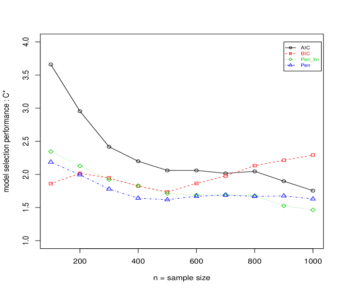
Figure 2. Model selection performance ($C^{*}$) as a function of sample size n, with each penalty, Mod1.

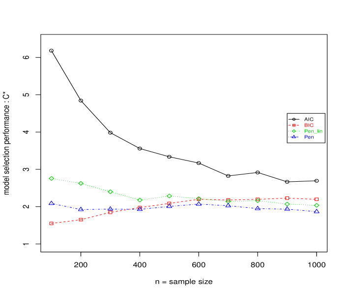
Figure 3. Model selection performance ($C^{*}$) as a function of sample size n, with each penalty, Mod2.

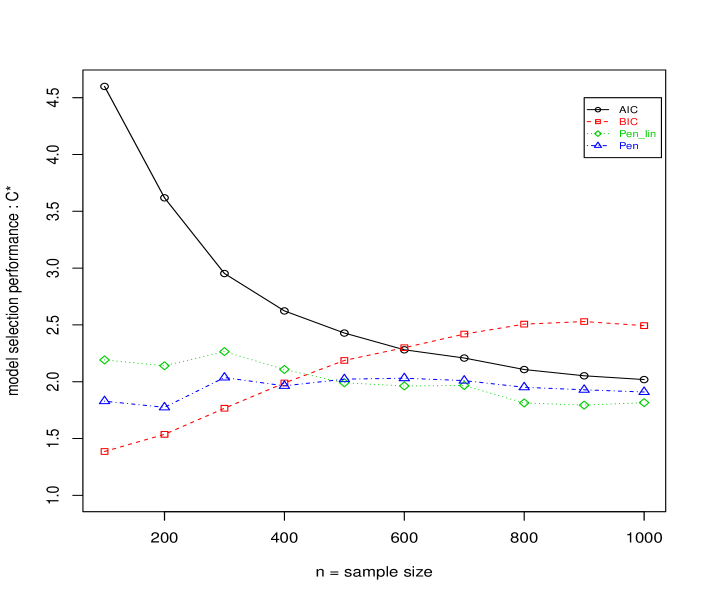
Figure 4. Model selection performance ($C^{*}$) as a function of sample size n, with each penalty, Mod3.

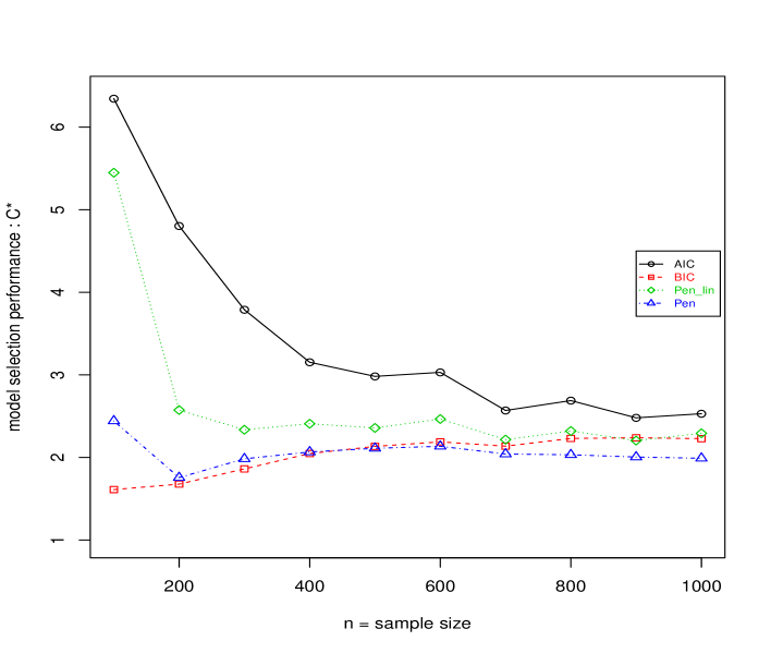
Figure 5. Model selection performance ($C^{*}$) as a function of sample size n, with each penalty, Mod4.

6. Proofs

6.1. Notations and technical tools

Subsequently we will use the following notations. Denote by $\parallel f\parallel_{n}$ and $\langle f,g\rangle_{n}$ the empirical euclidian norm and the inner product

$$\parallel f\parallel_{n}^{2}=\frac{1}{n}\sum_{i=1}^{n}f^{2}(x_{i}),\mbox{ and }\langle f,g\rangle_{n}=\frac{1}{n}\sum_{i=1}^{n}f(x_{i})g(x_{i}).$$

Note that $\parallel.\parallel_{n}$ is a semi norm on the space $\mathcal{F}$ of functions $g:\mathcal{X}\longrightarrow\mathbb{R}$, but is a norm in the quotient space $\mathcal{F}/\mathcal{R}$ associated to the equivalence relation $\mathcal{R}$ : $g~{}\mathcal{R}~{}h$ if and only if $g(x_{i})=h(x_{i})$ for all $i\in\{1,\dots,n\}$. It follows from (2.3) that $\gamma$ defined in (2.4) can be expressed as the sum of a centered empirical process and of the estimation criterion $\gamma_{n}$. More precisely, denoting by $\vec{\varepsilon}=(\varepsilon_{1},\cdots,\varepsilon_{n})^{T}$, with $\varepsilon_{i}=Y_{i}-\mathbb{E}_{f_{0}}(Y_{i}),$ for all $f$, we have

(6.1) $$\gamma(f)=\gamma_{n}(f)+\frac{1}{n}\sum_{i=1}^{n}\varepsilon_{i}f(x_{i}):=\gamma_{n}(f)+\langle\vec{\varepsilon},f\rangle_{n}.$$

Easy calculations show that for $\gamma$ defined in (2.4) we have,

$$\mathcal{K}(\mathbb{P}_{f_{0}}^{(n)},\mathbb{P}_{f}^{(n)}) = \frac{1}{n}\int\log\left(\frac{\mathbb{P}_{f_{0}}^{(n)}}{\mathbb{P}_{f}^{(n)}}\right)d\mathbb{P}_{f_{0}}^{(n)}=\gamma(f)-\gamma(f_{0})$$

$$= \frac{1}{n}\sum_{i=1}^{n}\left[\pi_{f_{0}}(x_{i})\log\left(\frac{\pi_{f_{0}}(x_{i})}{\pi_{f}(x_{i})}\right)+(1-\pi_{f_{0}}(x_{i}))\log\left(\frac{1-\pi_{f_{0}}(x_{i})}{1-\pi_{f}(x_{i})}\right)\right].$$

Let us recall the usual bounds (see Castellan Castellan2003) for kullback-Leibler information:

Lemma 6.1.

For positive densities $p$ and $q$ with respect to $\mu$, if $f=\log(q/p)$, then

$$\frac{1}{2}\int f^{2}(1\wedge e^{f})p\,d\mu\leqslant\mathcal{K}(p,q)\leqslant\frac{1}{2}\int f^{2}(1\vee e^{f})p\,d\mu.$$

6.2. Proof of Proposition 3.1:

By definition of $\hat{f}_{m}$, for all $f\in S_{m}\cap\mathbb{L}_{\infty}(C_{0})$, $\gamma_{n}(\hat{f}_{m})-\gamma_{n}(f)\leqslant 0.$ We apply (6.1), with $f=f_{m}$ and $f=\hat{f}_{m}$,

$$\gamma(\hat{f}_{m})-\gamma(f_{0})\leqslant\gamma(f_{m})-\gamma(f_{0})+\langle\vec{\varepsilon},\hat{f}_{m}-f_{m}\rangle_{n}.$$

As usual, the main part of the proof relies on the study of the empirical process $\langle\vec{\varepsilon},\hat{f}_{m}-f_{m}\rangle_{n}$. Since $\hat{f}_{m}-f_{m}$ belongs to $S_{m}$, $\hat{f}_{m}-f_{m}=\sum_{j=1}^{D_{m}}\alpha_{j}\psi_{j}$, where $\{\psi_{1},\dots,\psi_{D_{m}}\},$ is an orthonormal basis of $S_{m}$ and consequently

$$\langle\vec{\varepsilon},\hat{f}_{m}-f_{m}\rangle_{n}=\sum_{j=1}^{D_{m}}\alpha_{j}\langle\vec{\varepsilon},\psi_{j}\rangle_{n}.$$

Applying Cauchy-Schwarz inequality we get

$$\langle\vec{\varepsilon},\hat{f}_{m}-f_{m}\rangle_{n} \leqslant \sqrt{\sum_{j=1}^{D_{m}}\alpha_{j}^{2}}\sqrt{\sum_{j=1}^{D_{m}}\left(\langle\vec{\varepsilon},\psi_{j}\rangle_{n}\right)^{2}}$$

$$= \lVert\hat{f}_{m}-f_{m}\rVert_{n}\sqrt{\sum_{j=1}^{D_{m}}\left(\frac{1}{n}\sum_{i=1}^{n}\varepsilon_{i}\psi_{j}(x_{i})\right)^{2}}.$$

We now apply Lemma 6.2 (See Section 7 for the proof of Lemma 6.2)

Lemma 6.2.

Let $\mathcal{S}_{m}$ the model defined in (2.5) and $\{\psi_{1},\dots,\psi_{D_{m}}\}$ an orthonormal basis of the linear span $\{\phi_{k},~{}k\in m\}$. We also denote by $\Lambda_{m}$ the set of $\beta=(\beta_{1},...,\beta_{D})$ such that $f_{\beta}(.)=\sum_{j=1}^{D}\beta_{j}\psi_{j}(.)$ satisfies $f_{\beta}\in\mathcal{S}_{m}\cap\mathbb{L}_{\infty}(C_{0})$. Let $\beta^{*}$ be any minimizer of the function $\beta\rightarrow\gamma(f_{\beta})$ over $\Lambda_{m}$, we have

(6.2) $$\frac{\mathcal{U}_{0}^{2}}{2}\lVert f_{\beta}-f_{\beta^{*}}\rVert^{2}_{n}\leq\gamma(f_{\beta})-\gamma(f_{\beta^{*}}),$$

where $\mathcal{U}_{0}=e^{C_{0}}/(1+e^{C_{0}})^{2}$.

Then we have

$$\langle\vec{\varepsilon},\hat{f}_{m}-f_{m}\rangle_{n}\quad\leqslant\quad\sqrt{\sum_{j=1}^{D_{m}}\left(\langle\vec{\varepsilon},\psi_{j}\rangle_{n}\right)^{2}}\frac{\sqrt{2}}{\mathcal{U}_{0}}\sqrt{\gamma(\hat{f}_{m})-\gamma(f_{m})}$$

Now we use that for every positive numbers, $a$, $b$, $x$, $ab\leqslant(x/2)a^{2}+[1/(2x)]b^{2}$, and infer that

$$\gamma(\hat{f}_{m})-\gamma(f_{0})\leq\gamma(f_{m})-\gamma(f_{0})+\frac{x}{\mathcal{U}_{0}^{2}}\sum_{j=1}^{D_{m}}\left(\langle\vec{\varepsilon},\psi_{j}\rangle_{n}\right)^{2}+(1/2x)(\gamma(\hat{f}_{m})-\gamma(f_{m})).$$

For $x>1/2$, it follows that

$$\mathbb{E}_{f_{0}}[\gamma(\hat{f}_{m})-\gamma(f_{0})]\leqslant\gamma(f_{m})-\gamma(f_{0})+\frac{2x^{2}}{(2x-1)\mathcal{U}_{0}^{2}}\mathbb{E}_{f_{0}}\left[\sum_{j=1}^{D_{m}}\left(\langle\vec{\varepsilon},\psi_{j}\rangle_{n}\right)^{2}\right].$$

We conclude the proof by using that

$$\mathbb{E}_{f_{0}}\left[\sum_{j=1}^{D_{m}}\left(\langle\vec{\varepsilon},\psi_{j}\rangle_{n}\right)^{2}\right]\leqslant\frac{D_{m}}{4n}.$$

∎

6.3. Proof of Theorem 3.1

By definition, for all $m\in\mathcal{M}$,

$$\gamma_{n}(\hat{f}_{\hat{m}})+\mbox{pen}(\hat{m})\leqslant\gamma_{n}(\hat{f_{m}})+\mbox{pen}(m)\leqslant\gamma_{n}(f_{m})+\mbox{pen}(m).$$

Applying (6.1) we have

(6.3) $$\mathcal{K}(\mathbb{P}_{f_{0}}^{(n)},\mathbb{P}_{\hat{f}_{\hat{m}}}^{(n)})\leqslant\mathcal{K}(\mathbb{P}_{f_{0}}^{(n)},\mathbb{P}_{f_{m}}^{(n)})+\langle\vec{\varepsilon},\hat{f}_{\hat{m}}-f_{m}\rangle_{n}+\mbox{pen}(m)-\mbox{pen}(\hat{m}).$$

It remains to study $\langle\vec{\varepsilon},\hat{f}_{\hat{m}}-f_{m}\rangle_{n}$, using the following lemma, which is a modification of Lemma 1 in Durot et al. DurotLebarbierTocquet.

Lemma 6.3.

For every $D$, $D^{\prime}$ and $x\geqslant 0$ we have

$$\mathbb{P}\left(\sup_{u\in\big{(}S_{D}\cap\mathbb{L}_{\infty}(C_{0})+S_{D^{\prime}}\cap\mathbb{L}_{\infty}(C_{0})\Big{)}}\frac{\langle\vec{\varepsilon},u\rangle_{n}}{\parallel u\parallel_{n}}\rangle\sqrt{\frac{D+D^{\prime}}{4n}}+\sqrt{\frac{5x}{n}}\right)\leqslant\exp{(-x)}.$$

Fix $\xi>0$ and let $\Omega_{\xi}(m)$ denote the event

$$\Omega_{\xi}(m)=\bigcap_{m^{\prime}\in\mathcal{M}}\left\{\sup_{u\in\Big{(}S_{m}\cap\mathbb{L}_{\infty}(C_{0})+S_{m^{\prime}}\cap\mathbb{L}_{\infty}(C_{0})\Big{)}}\frac{\langle\vec{\varepsilon},u\rangle_{n}}{\parallel u\parallel_{n}}\leq\sqrt{\frac{D_{m}+D_{m^{\prime}}}{4n}}+\sqrt{5(L_{m^{\prime}}D_{m^{\prime}}+\xi)/n}\right\}.$$

Then we have

(6.4) $$\mathbb{P}\left(\Omega_{\xi}(m)\right)\geqslant 1-\Sigma\exp(-\xi).$$

See the Appendix for the proof of this lemma. Fix $\xi>0$, applying Lemma 6.3, we infer that on the event $\Omega_{\xi}(m),$

$$\langle\vec{\varepsilon},\hat{f}_{\hat{m}}-f_{m}\rangle_{n} \leqslant\left(\sqrt{\frac{D_{m}+D_{\hat{m}}}{4n}}+\sqrt{5\frac{L_{\hat{m}}D_{\hat{m}}+\xi}{n}}\right)\parallel\hat{f}_{\hat{m}}-f_{m}\parallel_{n}$$

$$\leqslant\left(\sqrt{\frac{D_{m}+D_{\hat{m}}}{4n}}+\sqrt{5\frac{L_{\hat{m}}D_{\hat{m}}+\xi}{n}}\right)\left(\parallel\hat{f}_{\hat{m}}-f_{0}\parallel_{n}+\parallel f_{0}-f_{m}\parallel_{n}\right)$$

$$\leqslant\left(\sqrt{D_{\hat{m}}}\left(\frac{1}{\sqrt{4n}}+\sqrt{\frac{5L_{\hat{m}}}{n}}\right)+\sqrt{\frac{D_{m}}{4n}}+\sqrt{5\frac{\xi}{n}}\right)\left(\parallel\hat{f}_{\hat{m}}-f_{0}\parallel_{n}+\parallel f_{0}-f_{m}\parallel_{n}\right).$$

Applying that $2xy\leqslant\theta x^{2}+\theta^{-1}y^{2}$, for all $x>0$, $y>0$, $\theta>0$, we get that on $\Omega_{\xi}(m)$ and for every $\eta\in]0,1[$

$$\langle\vec{\varepsilon},\hat{f}_{\hat{m}}-f_{m}\rangle_{n}\!\!\! \leqslant \!\!\!(\frac{1-\eta}{2})\left[(1+\eta)\parallel\hat{f}_{\hat{m}}-f_{0}\parallel_{n}^{2}+(1+\eta^{-1})\parallel f_{0}-f_{m}\parallel_{n}^{2}\right]$$

$$+ \frac{1}{2(1-\eta)}\left[(1+\eta)D_{\hat{m}}\left(\frac{1}{\sqrt{4n}}+\sqrt{\frac{5L_{\hat{m}}}{n}}\right)^{2}+(1+\eta^{-1})\left(\sqrt{\frac{D_{m}}{4n}}+\sqrt{\frac{5\xi}{n}}\right)^{2}\right]$$

$$\leqslant \!\!\!\frac{1-\eta^{2}}{2}\parallel\hat{f}_{\hat{m}}-f_{0}\parallel_{n}^{2}+\frac{\eta^{-1}-\eta}{2}\parallel f_{0}-f_{m}\parallel_{n}^{2}+\frac{1+\eta}{2(1-\eta)}D_{\hat{m}}\left(\frac{1}{\sqrt{4n}}+\sqrt{\frac{5L_{\hat{m}}}{n}}\right)^{2}$$

$$+\frac{1+\eta^{-1}}{1-\eta}\Big{(}\frac{D_{m}}{4n}+\frac{5\xi}{n}\Big{)}.$$

If $\mbox{pen}(m)\geqslant\Big{(}\lambda D_{m}\left(\frac{1}{2}+\sqrt{5L_{m}}\right)^{2}\Big{)}/n,$ with $\lambda>0$, we have

$$\langle\vec{\varepsilon},\hat{f}_{\hat{m}}-f_{m}\rangle_{n}\!\!\! \leqslant \!\!\!\frac{1-\eta^{2}}{2}\parallel\hat{f}_{\hat{m}}-f_{0}\parallel_{n}^{2}+\frac{\eta^{-1}-\eta}{2}\parallel f_{0}-f_{m}\parallel_{n}^{2}+\frac{1+\eta}{2(1-\eta)\lambda}\mbox{pen}(\hat{m})+\frac{1+\eta^{-1}}{(1-\eta)\lambda}\mbox{pen(m)}$$

$$+\frac{1+\eta^{-1}}{1-\eta}\frac{5\xi}{n}.$$

It follows from (6.3) that

$$\mathcal{K}(\mathbb{P}_{f_{0}}^{(n)},\mathbb{P}_{\hat{f}_{\hat{m}}}^{(n)}) \leqslant \mathcal{K}(\mathbb{P}_{f_{0}}^{(n)},\mathbb{P}_{f_{m}}^{(n)})+\frac{1-\eta^{2}}{2}\parallel\hat{f}_{\hat{m}}-f_{0}\parallel_{n}^{2}+\frac{\eta^{-1}-\eta}{2}\parallel f_{0}-f_{m}\parallel_{n}^{2}$$

$$+\frac{1+\eta}{2(1-\eta)\lambda}\mbox{pen}(\hat{m})+\frac{1+\eta^{-1}}{(1-\eta)\lambda}\mbox{pen(m)}+\frac{1+\eta^{-1}}{1-\eta}\frac{5\xi}{n}+\mbox{pen}(m)-\mbox{pen}(\hat{m}).$$

Taking $\lambda=(\eta+1)/(2(1-\eta))$, we have

$$\mathcal{K}(\mathbb{P}_{f_{0}}^{(n)},\mathbb{P}_{\hat{f}_{\hat{m}}}^{(n)})\leqslant\mathcal{K}(\mathbb{P}_{f_{0}}^{(n)},\mathbb{P}_{f_{m}}^{(n)})\\ +\frac{4\lambda}{(2\lambda+1)^{2}}\parallel\hat{f}_{\hat{m}}-f_{0}\parallel_{n}^{2}+\frac{4\lambda}{4\lambda^{2}-1}\parallel f_{0}-f_{m}\parallel_{n}^{2}+\frac{6\lambda+1}{2\lambda-1}\mbox{pen}(m)+\frac{10\lambda(2\lambda+1)}{2\lambda-1}\frac{\xi}{n}.$$

Now we use the following lemma (see Lemma 6.1 in Kwemou kwemou) that allows to connect empirical norm and Kullback-Leibler divergence.

Lemma 6.4.

Under Assumptions ($\mathbf{A_{1}}$), for all $m\in\mathcal{M}$ and all $t\in S_{m}\cap\mathbb{L}_{\infty}(C_{0})$, we have

$$c_{min}\lVert t-f_{0}\rVert_{n}^{2}\leqslant\mathcal{K}(\mathbb{P}_{f_{0}}^{(n)},\mathbb{P}_{t}^{(n)})\leqslant c_{max}\lVert t-f_{0}\rVert_{n}^{2}.$$

where $c_{min}$ and $c_{max}$ are constants depending on $C_{0}$ and $c_{1}.$

Consequently

$$\mathcal{K}(\mathbb{P}_{f_{0}}^{(n)},\mathbb{P}_{\hat{f}_{\hat{m}}}^{(n)})\leqslant C(c_{min})\left\{\mathcal{K}(\mathbb{P}_{f_{0}}^{(n)},\mathbb{P}_{f_{m}}^{(n)})+\mbox{pen}(m)\right\}+C_{1}(c_{min})\frac{\xi}{n},$$

where

$$C(c_{min})=\max\left\{\frac{1+\frac{4\lambda}{(4\lambda^{2}-1)c_{min}}}{1-\frac{4\lambda}{c_{min}(2\lambda+1)^{2}}};\frac{\frac{6\lambda+1}{2\lambda-1}}{1-\frac{4\lambda}{c_{min}(2\lambda+1)^{2}}}\right\}~{}\mbox{and}~{}~{}C_{1}(c_{min})=\frac{\frac{10\lambda(2\lambda+1)}{2\lambda-1}}{1-\frac{4\lambda}{c_{min}(2\lambda+1)^{2}}}.$$

Thus we take $\lambda$ such that

(6.5) $$1-\frac{4\lambda}{c_{min}(2\lambda+1)^{2}}>0,$$

where $c_{min}$ depends on the bound of the true function $f_{0}$. By definition of $\Omega_{\xi}(m)$ and (6.4), there exists a random variable $V\geqslant 0$ with $\mathbb{P}(V>\xi)\leqslant\Sigma\exp{(-\xi)}$ and $\mathbb{E}_{f_{0}}(V)\leqslant\Sigma,$ such that

$$\mathcal{K}(\mathbb{P}_{f_{0}}^{(n)},\mathbb{P}_{\hat{f}_{\hat{m}}}^{(n)})\leqslant C(c_{min})\left\{\mathcal{K}(\mathbb{P}_{f_{0}}^{(n)},\mathbb{P}_{f_{m}}^{(n)})+\mbox{pen}(m)\right\}+C_{1}(c_{min})\frac{V}{n},$$

which implies that for all $m\in\mathcal{M}$,

$$\mathbb{E}_{f_{0}}[\mathcal{K}(\mathbb{P}_{f_{0}}^{(n)},\mathbb{P}_{\hat{f}_{\hat{m}}}^{(n)})]\leqslant C(c_{min})\left\{\mathcal{K}(\mathbb{P}_{f_{0}}^{(n)},\mathbb{P}_{f_{m}}^{(n)})+\mbox{pen}(m)\right\}+C_{1}(c_{min})\frac{\Sigma}{n}.$$

This concludes the proof. ∎

6.4. Proof of Proposition 4.1:

Let $f_{m}$, $\hat{f}_{m}$, $\pi_{f_{m}}$ and $\pi_{\hat{f}_{m}}$ given in Lemma 4.1, proved in appendix. In the following, $D_{m}=|m|.$ For $\delta>0$, let $\Omega_{m}(\delta)$ be the event

(6.6) $$\Omega_{m}(\delta)=\bigcap_{J\in m}\left\{\left|\frac{\pi_{\hat{f}_{m}}^{(J)}}{\pi_{f_{m}}^{(J)}}-1\right|\leqslant\delta\right\}\bigcap\left\{\left|\frac{1-\pi_{\hat{f}_{m}}^{(J)}}{1-\pi_{f_{m}}^{(J)}}-1\right|\leqslant\delta\right\}.$$

According to pythagore’s type identity and Lemma 4.1 we write

$$\mathcal{K}(\mathbb{P}_{f_{0}}^{(n)},\mathbb{P}_{\hat{f_{m}}}^{(n)})=\mathcal{K}(\mathbb{P}_{f_{0}}^{(n)},\mathbb{P}_{f_{m}}^{(n)})+\mathcal{K}(\mathbb{P}_{f_{m}}^{(n)},\mathbb{P}_{\hat{f_{m}}}^{(n)}){{{1}}{\mathrm{I}}}_{\Omega_{m}(\delta)}+\mathcal{K}(\mathbb{P}_{f_{m}}^{(n)},\mathbb{P}_{\hat{f_{m}}}^{(n)}){{{1}}{\mathrm{I}}}_{\Omega_{m}^{c}(\delta)},$$

where

$$\mathcal{K}(\mathbb{P}_{f_{m}}^{(n)},\mathbb{P}_{\hat{f_{m}}}^{(n)})\!\!\! = \!\!\!\frac{1}{n}\sum_{i=1}^{n}\left[\pi_{f_{m}}(x_{i})\log\left(\frac{\pi_{f_{m}}(x_{i})}{\pi_{\hat{f}_{m}}(x_{i})}\right)+(1-\pi_{f_{m}}(x_{i}))\log\left(\frac{1-\pi_{f_{m}}(x_{i})}{1-\pi_{\hat{f}_{m}}(x_{i})}\right)\right]$$

$$= \!\!\!\frac{1}{n}\sum_{J\in m}|J|\left[\pi_{f_{m}}^{(J)}\log\left(\frac{\pi_{f_{m}}^{(J)}}{\pi_{\hat{f}_{m}}^{(J)}}\right)+(1-\pi_{f_{m}}^{(J)})\log\left(\frac{1-\pi_{f_{m}}^{(J)}}{1-\pi_{\hat{f}_{m}}^{(J)}}\right)\right].$$

The first step consists in showing that

(6.8) $$\frac{1-\delta}{2(1+\delta)^{2}}\mathcal{X}_{m}^{2}{{{1}}{\mathrm{I}}}_{\Omega_{m}(\delta)}\leqslant\mathcal{K}(\mathbb{P}_{f_{m}}^{(n)},\mathbb{P}_{\hat{f_{m}}}^{(n)}){{{1}}{\mathrm{I}}}_{\Omega_{m}(\delta)}\leqslant\frac{1+\delta}{2(1-\delta)^{2}}\mathcal{X}_{m}^{2}{{{1}}{\mathrm{I}}}_{\Omega_{m}(\delta)},$$

where

(6.9) $$\mathcal{X}_{m}^{2}=\frac{1}{n}\sum_{J\in m}\frac{(\sum_{k\in J}\varepsilon_{k})^{2}}{|J|\pi_{f_{m}}^{(J)}[1-\pi_{f_{m}}^{(J)}]},\mbox{ with }\qquad\frac{4\rho^{2}D_{m}}{n}\leqslant\mathbb{E}_{f_{0}}[\mathcal{X}_{m}^{2}]\leqslant\frac{2D_{m}}{n}.$$

The second step relies on the proof of

(6.10) $$\big{|}\mathbb{E}_{f_{0}}\left(\mathcal{K}(\mathbb{P}_{f_{m}}^{(n)},\mathbb{P}_{\hat{f_{m}}}^{(n)}){{{1}}{\mathrm{I}}}_{\Omega_{m}^{c}(\delta)}\right)\Big{|}\leqslant 2\log\left(\frac{1}{\rho}\right)\mathbb{P}[\Omega_{m}^{c}(\delta)].$$

The last step consists in showing that for $\epsilon>0$, since for all $J\in m$, $|J|\geq\Gamma[\log(n)]^{2}$, where $\Gamma>0$ is an absolute constant, then we have

(6.11) $$\mathbb{P}[\Omega_{m}^{c}(\delta)]\leqslant 4|m|\exp\left(-\frac{\delta^{2}}{2(1+\delta/3)}\rho^{2}\Gamma[\log(n)]^{2}\right)\leq\frac{\kappa(\rho,\delta,\Gamma,\epsilon)}{n^{(1+\epsilon)}}.$$

Gathering (6.8)-(6.11), we conclude that

$$\mathbb{E}_{f_{0}}[\mathcal{K}(\mathbb{P}_{f_{0}}^{(n)},\mathbb{P}_{\hat{f_{m}}}^{(n)})] \leqslant \mathcal{K}(\mathbb{P}_{f_{0}}^{(n)},\mathbb{P}_{f_{m}}^{(n)})+\frac{(1+\delta)|m|}{(1-\delta)^{2}n}+2\log\left(\frac{1}{\rho}\right)\mathbb{P}[\Omega_{m}^{c}(\delta)]$$

$$\leqslant \mathcal{K}(\mathbb{P}_{f_{0}}^{(n)},\mathbb{P}_{f_{m}}^{(n)})+\frac{(1+\delta)|m|}{(1-\delta)^{2}n}+\frac{\kappa(\rho,\delta,\Gamma,\epsilon)}{n^{(1+\epsilon)}}.$$

We finish by proving (6.8), (6.9), (6.10) and (6.11).

$\bullet$ Proof of (6.8) and (6.9) :

Arguing as in Castellan Castellan2003 and using Lemma 6.1 we have

$$\mathcal{K}(\mathbb{P}_{f_{m}}^{(n)},\mathbb{P}_{\hat{f_{m}}}^{(n)})\!\!\! \geqslant \!\!\!\frac{1}{2n}\sum_{J\in m}|J|\left[\pi_{f_{m}}^{(J)}\left(1\wedge\frac{\pi_{\hat{f}_{m}}^{(J)}}{\pi_{f_{m}}^{(J)}}\right)\log^{2}\left(\frac{\pi_{f_{m}}^{(J)}}{\pi_{\hat{f}_{m}}^{(J)}}\right)+(1-\pi_{f_{m}}^{(J)})\left(1\wedge\frac{1-\pi_{\hat{f}_{m}}^{(J)}}{1-\pi_{f_{m}}^{(J)}}\right)\log^{2}\left(\frac{1-\pi_{f_{m}}^{(J)}}{1-\pi_{\hat{f}_{m}}^{(J)}}\right)\right]$$

and

$$\mathcal{K}(\mathbb{P}_{f_{m}}^{(n)},\mathbb{P}_{\hat{f_{m}}}^{(n)})\!\!\! \leqslant \!\!\!\frac{1}{2n}\sum_{J\in m}|J|\left[\pi_{f_{m}}^{(J)}\left(1\vee\frac{\pi_{\hat{f}_{m}}^{(J)}}{\pi_{f_{m}}^{(J)}}\right)\log^{2}\left(\frac{\pi_{f_{m}}^{(J)}}{\pi_{\hat{f}_{m}}^{(J)}}\right)+(1-\pi_{f_{m}}^{(J)})\left(1\vee\frac{1-\pi_{\hat{f}_{m}}^{(J)}}{1-\pi_{f_{m}}^{(J)}}\right)\log^{2}\left(\frac{1-\pi_{f_{m}}^{(J)}}{1-\pi_{\hat{f}_{m}}^{(J)}}\right)\right].$$

It follows that

(6.12) $$\frac{1-\delta}{2}V^{2}(\pi_{f_{m}},\pi_{\hat{f}_{m}}){{{1}}{\mathrm{I}}}_{\Omega_{m}(\delta)}\leqslant\mathcal{K}(\mathbb{P}_{f_{m}}^{(n)},\mathbb{P}_{\hat{f_{m}}}^{(n)}){{{1}}{\mathrm{I}}}_{\Omega_{m}(\delta)}\leqslant\frac{1+\delta}{2}V^{2}(\pi_{f_{m}},\pi_{\hat{f}_{m}}){{{1}}{\mathrm{I}}}_{\Omega_{m}(\delta)},$$

where $V^{2}(\pi_{f_{m}},\pi_{\hat{f}_{m}})$ is defined by

(6.13) $$V^{2}(\pi_{f_{m}},\pi_{\hat{f}_{m}})=\frac{1}{n}\sum_{J\in m}|J|\frac{[\pi_{\hat{f}_{m}}^{(J)}-\pi_{f_{m}}^{(J)}]^{2}}{\pi_{f_{m}}^{(J)}}\left[\frac{\log[\pi_{\hat{f}_{m}}^{(J)}/\pi_{f_{m}}^{(J)}]}{\pi_{\hat{f}_{m}}^{(J)}/\pi_{f_{m}}^{(J)}-1}\right]^{2}\\ +\frac{1}{n}\sum_{J\in m}|J|\frac{[\pi_{\hat{f}_{m}}^{(J)}-\pi_{f_{m}}^{(J)}]^{2}}{1-\pi_{f_{m}}^{(J)}}\left[\frac{\log[(1-\pi_{\hat{f}_{m}}^{(J)})/(1-\pi_{f_{m}}^{(J)})]}{(1-\pi_{\hat{f}_{m}}^{(J)})/(1-\pi_{f_{m}}^{(J)})-1}\right]^{2}.$$

Now we use that, for all $x>0$,

(6.14) $$\frac{1}{1\vee x}\leqslant\frac{\log(x)}{x-1}\leqslant\frac{1}{1\wedge x}.$$

Hence we infer that

$$\frac{1}{(1+\delta)^{2}}\mathcal{X}_{m}^{2}{{{1}}{\mathrm{I}}}_{\Omega_{m}(\delta)}\leqslant V^{2}(\pi_{f_{m}},\pi_{\hat{f}_{m}}){{{1}}{\mathrm{I}}}_{\Omega_{m}(\delta)}\leqslant\frac{1}{(1-\delta)^{2}}\mathcal{X}_{m}^{2}{{{1}}{\mathrm{I}}}_{\Omega_{m}(\delta)},$$

with $\mathcal{X}_{m}^{2}$ defined in (6.9). This entails that (6.8) is proved. It remains now to check that

$$\frac{4\rho^{2}|m|}{n}\leqslant\mathbb{E}_{f_{0}}[\mathcal{X}_{m}^{2}]\leqslant\frac{2|m|}{n}.$$

According to Lemma 4.1 , for all partition $J\in m$ and for any $x_{i}\in J$,

$$\pi_{\hat{f}_{m}}(x_{i})=\pi_{\hat{f}_{m}}^{(J)},\qquad\mbox{ with } \qquad\pi_{\hat{f}_{m}}^{(J)}=\frac{1}{|J|}\sum_{i\in J}Y_{i},$$

$$\mbox{ and }\pi_{f_{m}}(x_{i})=\pi_{f_{m}}^{(J)},\qquad\mbox{ with } \pi_{f_{m}}^{(J)}=\frac{1}{|J|}\sum_{i\in J}\pi_{f_{0}}(x_{i}).$$

Consequently,

$$\mathcal{X}_{m}^{2}=\frac{1}{n}\sum_{J\in m}|J|\frac{(\sum_{k\in J}\varepsilon_{k})^{2}}{\sum_{k\in J}\pi_{f_{0}}(x_{k})[|J|-\sum_{k\in J}\pi_{f_{0}}(x_{k})]}=\frac{1}{n}\sum_{J\in m}\frac{(\sum_{k\in J}\varepsilon_{k})^{2}}{|J|\pi_{f_{m}}^{(J)}[1-\pi_{f_{m}}^{(J)}]},$$

and finally

$$\mathbb{E}_{f_{0}}(\mathcal{X}_{m}^{2})=\frac{1}{n}\sum_{J\in m}\mathbb{E}\left(\frac{(\sum_{k\in J}\varepsilon_{k})^{2}}{|J|\pi_{f_{m}}^{(J)}[1-\pi_{f_{m}}^{(J)}]}\right)=\frac{1}{n}\sum_{J\in m}\left(\frac{1}{|J|\pi_{f_{m}}^{(J)}[1-\pi_{f_{m}}^{(J)}]}\right)\sum_{k\in J}\mbox{Var}\left(Y_{k}\right).$$

Consequently

$$\mathbb{E}_{f_{0}}(\mathcal{X}_{m}^{2})=\frac{1}{n}\sum_{J\in m}\frac{\sum_{i\in J}\pi_{f_{0}}(x_{i})(1-\pi_{f_{0}}(x_{i}))}{|J|\pi_{f_{m}}^{(J)}[1-\pi_{f_{m}}^{(J)}]}.$$

Now, according to Assumption ($\mathbf{A_{2}}$), and Lemma 4.1, for all partition $m$, all $J\in m$, and all $x_{i}\in J$

$$0<\rho^{2}\leqslant\pi_{f_{0}}(x_{i})(1-\pi_{f_{0}}(x_{i}))\leqslant 1/4,\mbox{ and }0<\rho\leqslant\pi_{f_{m}}^{(J)}\mbox{ and }0<\rho\leqslant(1-\pi_{f_{m}}^{(J)}).$$

It follows that

$$4\rho^{2}\ \leqslant\frac{\sum_{k\in J}\pi_{f_{0}}(x_{k})(1-\pi_{f_{0}}(x_{k}))}{|J|\pi_{f_{m}}^{(J)}[1-\pi_{f_{m}}^{(J)}]}=\frac{\sum_{k\in J}\pi_{f_{0}}(x_{k})(1-\pi_{f_{0}}(x_{k}))}{|J|\pi_{f_{m}}^{(J)}}+\frac{\sum_{k\in J}\pi_{f_{0}}(x_{k})(1-\pi_{f_{0}}(x_{k}))}{|J|[1-\pi_{f_{m}}^{(J)}]}\leqslant 2,$$

and thus

$$\frac{4\rho^{2}|m|}{n}\leqslant\frac{1}{n}\sum_{J\in m}\frac{\sum_{i\in J}\pi_{f_{0}}(x_{i})(1-\pi_{f_{0}}(x_{i}))}{|J|\pi_{f_{m}}^{(J)}[1-\pi_{f_{m}}^{(J)}]}\leqslant\frac{2|m|}{n}.$$

In other words,

$$\frac{4\rho^{2}|m|}{n}\leqslant\mathbb{E}_{f_{0}}(\mathcal{X}_{m}^{2})\leqslant\frac{2|m|}{n}.$$

The ends up the proof of (6.8) and (6.9).

$\bullet$ Proof of (6.10) :

We start from (6.4), apply Assumption ($\mathbf{A_{2}}$) and Lemma 4.1, to obtain that and (6.10) is checked since

$$|\mathbb{E}\left(\mathcal{K}(\mathbb{P}_{f_{m}}^{(n)},\mathbb{P}_{\hat{f_{m}}}^{(n)}){{{1}}{\mathrm{I}}}_{\Omega_{m}^{c}(\delta)}\right)| \leqslant \frac{1}{n}\sum_{i=1}^{n}\mathbb{E}\left|\left[\log\left(\frac{\pi_{f_{m}}(x_{i})}{\pi_{\hat{f}_{m}}(x_{i})}\right){{{1}}{\mathrm{I}}}_{\Omega_{m}^{c}(\delta)}\right]\right|+\frac{1}{n}\sum_{i=1}^{n}\mathbb{E}\left|\left[\log\left(\frac{(1-\pi_{f_{m}}(x_{i}))}{(1-\pi_{\hat{f}_{m}}(x_{i}))}\right){{{1}}{\mathrm{I}}}_{\Omega_{m}^{c}(\delta)}\right]\right|$$

$$\leqslant 2\log\left(\frac{1}{\rho}\right)\mathbb{P}[\Omega_{m}^{c}(\delta)].$$

$\bullet$ Proof of (6.11):

We come to the control of $\mathbb{P}_{f_{0}}[\Omega_{m}^{c}(\delta)]$. Since

$$\mathbb{P}[\Omega_{m}^{c}(\delta)] \leqslant \sum_{J\in m}\mathbb{P}\left\{\left|\frac{\pi_{\hat{f}_{m}}^{(J)}}{\pi_{f_{m}}^{(J)}}-1\right|\geqslant\delta\right\}+\sum_{J\in m}\mathbb{P}\left\{\left|\frac{1-\pi_{\hat{f}_{m}}^{(J)}}{1-\pi_{f_{m}}^{(J)}}-1\right|\geqslant\delta\right\},$$

by applying Lemma 4.1, we infer that

$$\mathbb{P}\left\{\left|\frac{\pi_{\hat{f}_{m}}^{(J)}}{\pi_{f_{m}}^{(J)}}-1\right|\geqslant\delta\right\} = \mathbb{P}\left\{\left|\frac{\sum_{k\in J}\varepsilon_{k}}{\sum_{k\in J}\pi_{f_{0}}(x_{k})}\right|\geqslant\delta\right\}=\mathbb{P}\left\{\left|\sum_{k\in J}\varepsilon_{k}\right|\geqslant\delta\sum_{k\in J}\pi_{f_{0}}(x_{k})\right\},$$

and

$$\mathbb{P}\left\{\left|\frac{1-\pi_{\hat{f}_{m}}^{(J)}}{1-\pi_{f_{m}}^{(J)}}-1\right|\geqslant\delta\right\} = \mathbb{P}\left\{\left|\frac{\sum_{k\in J}\varepsilon_{k}}{\sum_{k\in J}(1-\pi_{f_{0}}(x_{k}))}\right|\geqslant\delta\right\}=\mathbb{P}\left\{\left|\sum_{k\in J}\varepsilon_{k}\right|\geqslant\delta\sum_{k\in J}(1-\pi_{f_{0}}(x_{k}))\right\}.$$

We write

$$\mathbb{P}\left\{\left|\sum_{k\in J}\varepsilon_{k}\right|\geqslant\delta\sum_{k\in J}\pi_{f_{0}}(x_{k})\right\}\!\!\! \leqslant \!\!\!\mathbb{P}\left\{\left|\sum_{k\in J}\varepsilon_{k}\right|\geqslant\delta\sum_{k\in J}\pi_{f_{0}}(x_{k})(1-\pi_{f_{0}}(x_{k}))\right\}$$

and

$$\mathbb{P}\left\{\left|\sum_{k\in J}\varepsilon_{k}\right|\geqslant\delta\sum_{k\in J}(1-\pi_{f_{0}}(x_{k}))\right\}\!\!\! \leqslant \!\!\!\mathbb{P}\left\{\left|\sum_{k\in J}\varepsilon_{k}\right|\geqslant\delta\sum_{k\in J}\pi_{f_{0}}(x_{k})(1-\pi_{f_{0}}(x_{k}))\right\}.$$

Then we have

$$\mathbb{P}[\Omega_{m}^{c}(\delta)] \leqslant 2\sum_{J\in m}\mathbb{P}\left\{\left|\sum_{k\in J}\varepsilon_{k}\right|\geqslant\delta\sum_{k\in J}\pi_{f_{0}}(x_{k})(1-\pi_{f_{0}}(x_{k}))\right\}.$$

Now, we apply Bernstein Concentration Inequality (see Massart massart2007 for example) to the right hand side of previous inequality, starting by recalling this Bernstein inequality.

Theorem 6.1.

Let $Z_{1},\cdots,Z_{n}$ be independent real valued random variables. Assume that there exist some positive numbers $v$ and $c$ such that for all $k\geqslant 2$,

$$\sum_{i=1}^{n}\mathbb{E}\left[|Z_{i}|^{k}\right]\leqslant\frac{k!}{2}vc^{k-2}.$$

Then for any positive $z$,

$$\mathbb{P}\left(\sum_{i=1}^{n}(Z_{i}-\mathbb{E}(Z_{i})\geqslant\sqrt{2vz}+cz\right)\leqslant\exp(-z),\mbox{ and }\mathbb{P}\left(\sum_{i=1}^{n}(Z_{i}-\mathbb{E}(Z_{i})\geqslant z\right)\leqslant\exp\left(-\frac{z^{2}}{2(v+cz)}\right).$$

Especially, if $|Z_{i}|\leqslant b$ for all $i$, then

(6.15) $$\mathbb{P}\left(\sum_{i=1}^{n}(Z_{i}-\mathbb{E}(Z_{i})\geqslant z\right)\leqslant\exp\left(-\frac{z^{2}}{2(\sum_{i=1}^{n}\mathbb{E}(Z_{i}^{2})+bz/3)}\right).$$

Applying (6.15) with $z=\delta\sum_{k\in J}\pi_{f_{0}}(x_{k})(1-\pi_{f_{0}}(x_{k}))$, $b=1$ and $v=\sum_{k\in J}\pi_{f_{0}}(x_{k})(1-\pi_{f_{0}}(x_{k})),$ we get that

$$\mathbb{P}\left\{\left|\sum_{k\in J}\varepsilon_{k}\right|\geqslant\delta\sum_{k\in J}\pi_{f_{0}}(x_{k})(1-\pi_{f_{0}}(x_{k}))\right\}$$

is less than

$$2\exp\left(-\frac{\delta^{2}[\sum_{k\in J}\pi_{f_{0}}(x_{k})(1-\pi_{f_{0}}(x_{k}))]^{2}}{2\left(\sum_{k\in J}\pi_{f_{0}}(x_{k})(1-\pi_{f_{0}}(x_{k}))+(\delta/3)\sum_{k\in J}\pi_{f_{0}}(x_{k})(1-\pi_{f_{0}}(x_{k}))\right)}\right),$$

and consequently

$$\mathbb{P}\left\{\left|\sum_{k\in J}\varepsilon_{k}\right|\geqslant\delta\sum_{k\in J}\pi_{f_{0}}(x_{k})(1-\pi_{f_{0}}(x_{k}))\right\}\!\!\! \leqslant \!\!\!2\exp\left[-\frac{\delta^{2}}{2(1+\delta/3)}\left(\sum_{k\in J}\pi_{f_{0}}(x_{k})(1-\pi_{f_{0}}(x_{k}))\right)\right]$$

$$\leqslant \!\!\!2\exp\left[-\frac{\delta^{2}}{2(1+\delta/3)}|J|\rho^{2}\right].$$

Consequently,

$$\mathbb{P}[\Omega_{m}^{c}(\delta)] \leqslant 4|m|\exp(-\Delta\rho^{2}\Gamma[\log(n)]^{2}),\qquad\mbox{ with }\qquad\Delta=\frac{\delta^{2}}{2(1+\delta/3)},$$

where $\Gamma$ is given by (4.1). For $\epsilon>0$ and $\delta$ such that

(6.16) $$\frac{\delta^{2}}{2(1+\delta/3)}\rho^{2}\Gamma\log(n)\geqslant 2+\epsilon,$$

using that $|m|\leqslant n$ implies that

$$4|m|\exp\left(-\frac{\delta^{2}}{2(1+\delta/3)}\rho^{2}\Gamma[\log(n)]^{2}\right)\leqslant\frac{\kappa}{n^{(1+\epsilon)}}.$$

And Result (6.11) follows.

6.5. Proof of Theorem 4.1

By definition, for all $m\in\mathcal{M}$,

$$\gamma_{n}(\hat{f}_{\hat{m}})+\mbox{pen}(\hat{m})\leqslant\gamma_{n}(\hat{f_{m}})+\mbox{pen}(m)\leqslant\gamma_{n}(f_{m})+\mbox{pen}(m).$$

Applying Formula (6.1), we have

(6.17) $$\gamma(\hat{f}_{\hat{m}})-\gamma(f_{0})\leqslant\gamma(f_{m})-\gamma(f_{0})+\langle\vec{\varepsilon},\hat{f}_{\hat{m}}-f_{m}\rangle_{n}+\mbox{pen}(m)-\mbox{pen}(\hat{m}).$$

Following Baraud Baraud2000 or Castellan Castellan2003, instead of bounding the supremum of the empirical process $\langle\vec{\varepsilon},\hat{f}_{\hat{m}}-f_{m}\rangle_{n}$, we split it in three terms. Let

$$\overline{\gamma}_{n}(t)={\gamma}_{n}(t)-\mathbb{E}_{f_{0}}(\gamma_{n}(t))=-<\vec{\varepsilon},f>_{n}$$

with $<\vec{\varepsilon},f>_{n}$ defined in (6.1), and write

$$\gamma(\hat{f}_{\hat{m}})-\gamma(f_{0}) \leqslant \gamma(f_{m})-\gamma(f_{0})+\mbox{pen}(m)-\mbox{pen}(\hat{m})$$

$$+\overline{\gamma}_{n}(f_{m})-\overline{\gamma}_{n}(f_{0})+\overline{\gamma}_{n}(f_{0})-\overline{\gamma}_{n}(f_{\hat{m}})+\overline{\gamma}_{n}(f_{\hat{m}})-\overline{\gamma}_{n}(\hat{f}_{\hat{m}}).$$

In other words,

(6.18) $$\mathcal{K}(\mathbb{P}_{f_{0}}^{(n)},\mathbb{P}_{\hat{f}_{\hat{m}}}^{(n)}) \leqslant \mathcal{K}(\mathbb{P}_{f_{0}}^{(n)},\mathbb{P}_{f_{m}}^{(n)})+\mbox{pen}(m)-\mbox{pen}(\hat{m})$$

$$+\overline{\gamma}_{n}(f_{m})-\overline{\gamma}_{n}(f_{0})+\overline{\gamma}_{n}(f_{0})-\overline{\gamma}_{n}(f_{\hat{m}})+\overline{\gamma}_{n}(f_{\hat{m}})-\overline{\gamma}_{n}(\hat{f}_{\hat{m}}).$$

The proof of Theorem 4.1 can be decomposed in three steps :

1. We prove that for $\epsilon>0,$

   $$\mathbb{E}_{f_{0}}\big{[}(\overline{\gamma}_{n}(f_{m})-\overline{\gamma}_{n}(f_{0})){{{1}}{\mathrm{I}}}_{\Omega_{m_{f}}(\delta)}\big{]}\leqslant\frac{\kappa^{\prime}(\rho,\delta,\Gamma,\epsilon)}{n^{(1+\epsilon)}}.$$

2. Let $\Omega_{1}(\xi)$ be the event

   $$\Omega_{1}(\xi)=\bigcap_{m^{\prime}\in\mathcal{M}}\left\{\chi_{m^{\prime}}^{2}{{{1}}{\mathrm{I}}}_{\Omega_{m_{f}}(\delta)}\right.\!\!\! \leqslant \!\!\!\left.\frac{2}{n}|m^{\prime}|+\frac{16}{n}\Big{(}1+\frac{\delta}{3}\Big{)}\sqrt{(L_{m^{\prime}}|m^{\prime}|+\xi)|m^{\prime}|}+\frac{8}{n}\Big{(}1+\frac{\delta}{3}\Big{)}(L_{m^{\prime}}|m^{\prime}|+\xi)\right\},$$

   where $(L_{m^{\prime}})_{m^{\prime}\in{\mathcal{M}}}$ satisfies Condition (4.2) and $m_{f}$ is given by Definition 4.1. For all $m^{\prime}$ in $\mathcal{M}$ we prove that on $\Omega_{1}(\xi)$

   (6.19) $$\Big{(}\overline{\gamma}_{n}(f_{m^{\prime}})-\overline{\gamma}_{n}(\hat{f}_{m^{\prime}})\Big{)}{{{1}}{\mathrm{I}}}_{\Omega_{m_{f}}(\delta)}\leqslant \frac{1}{2n}\Big{(}\frac{1+\delta}{1-\delta}\Big{)}|m^{\prime}|\Big{[}2+\Big{(}1+\frac{\delta}{3}\Big{)}\Big{(}2\delta+8L_{m^{\prime}}+16\sqrt{L_{m^{\prime}}}\Big{)}\Big{]}$$

   $$+\frac{4\xi}{n}\Big{(}\frac{1+\delta}{1-\delta}\Big{)}\Big{(}1+\frac{\delta}{3}\Big{)}\Big{(}1+\frac{4}{\delta}\Big{)}+\frac{1}{1+\delta}\mathcal{K}(\mathbb{P}_{f_{m^{\prime}}}^{(n)},\mathbb{P}_{\hat{f}_{m^{\prime}}}^{(n)}){{{1}}{\mathrm{I}}}_{\Omega_{m_{f}}(\delta)},$$

   and

   (6.20) $$\mathbb{P}(\Omega_{1}(\xi)^{c})\leqslant 2\Sigma e^{-\xi}.$$

3. Let $\Omega_{2}(\xi)$ be the event

   $$\Omega_{2}(\xi)=\bigcap_{m^{\prime}\in\mathcal{M}}\left[(\overline{\gamma}_{n}(f_{0})-\overline{\gamma}_{n}(f_{m^{\prime}}))\leqslant\mathcal{K}(\mathbb{P}_{f_{0}}^{(n)},\mathbb{P}_{f_{m^{\prime}}}^{(n)})-2h^{2}(\mathbb{P}_{f_{0}}^{(n)},\mathbb{P}_{f_{m^{\prime}}}^{(n)})+\frac{2}{n}(L_{m}^{\prime}|m^{\prime}|+\xi)\right].$$

   We prove that, $\mathbb{P}(\Omega_{2}(\xi)^{c})\leqslant\Sigma e^{-\xi}.$

Now, we will prove the result of Theorem 4.1 using (R-1), (R-2) and (R-3).
According to (6.18), we can write

$$\mathcal{K}(\mathbb{P}_{f_{0}}^{(n)},\mathbb{P}_{\hat{f}_{\hat{m}}}^{(n)}){{{1}}{\mathrm{I}}}_{\Omega_{m_{f}}(\delta)} \leqslant \mathcal{K}(\mathbb{P}_{f_{0}}^{(n)},\mathbb{P}_{f_{m}}^{(n)})+\mbox{pen}(m)-\mbox{pen}(\hat{m})$$

$$+(\overline{\gamma}_{n}(f_{m})-\overline{\gamma}_{n}(f_{0})){{{1}}{\mathrm{I}}}_{\Omega_{m_{f}}(\delta)}+(\overline{\gamma}_{n}(f_{0})-\overline{\gamma}_{n}(f_{\hat{m}})){{{1}}{\mathrm{I}}}_{\Omega_{m_{f}}(\delta)}+(\overline{\gamma}_{n}(f_{\hat{m}})-\overline{\gamma}_{n}(\hat{f}_{\hat{m}}){{{1}}{\mathrm{I}}}_{\Omega_{m_{f}}(\delta)}.$$

Combining (R-2) and (R-3) with $m^{\prime}=\hat{m}$, we infer that on $\Omega_{1}(\xi)\bigcap\Omega_{2}(\xi)$

$$\mathcal{K}(\mathbb{P}_{f_{0}}^{(n)},\mathbb{P}_{\hat{f}_{\hat{m}}}^{(n)}){{{1}}{\mathrm{I}}}_{\Omega_{m_{f}}(\delta)} \leqslant \mathcal{K}(\mathbb{P}_{f_{0}}^{(n)},\mathbb{P}_{f_{m}}^{(n)})+\mbox{pen}(m)-\mbox{pen}(\hat{m})+(\overline{\gamma}_{n}(f_{m})-\overline{\gamma}_{n}(f_{0})){{{1}}{\mathrm{I}}}_{\Omega_{m_{f}}(\delta)}$$

$$+\frac{1}{2n}\Big{(}\frac{1+\delta}{1-\delta}\Big{)}|\hat{m}|\Big{[}2+\Big{(}1+\frac{\delta}{3}\Big{)}\Big{(}2\delta+8L_{\hat{m}}+16\sqrt{L_{\hat{m}}}\Big{)}\Big{]}+2L_{\hat{m}}\frac{|\hat{m}|}{n}$$

$$+\frac{4\xi}{n}\Big{[}\frac{1}{2}+\Big{(}\frac{1+\delta}{1-\delta}\Big{)}\Big{(}1+\frac{\delta}{3}\Big{)}\Big{(}1+\frac{4}{\delta}\Big{)}\Big{]}$$

$$+\Big{[}\mathcal{K}(\mathbb{P}_{f_{0}}^{(n)},\mathbb{P}_{f_{\hat{m}}}^{(n)})-2h^{2}(\mathbb{P}_{f_{0}}^{(n)},\mathbb{P}_{f_{\hat{m}}}^{(n)})+\frac{1}{1+\delta}\mathcal{K}(\mathbb{P}_{f_{\hat{m}}}^{(n)},\mathbb{P}_{\hat{f}_{\hat{m}}}^{(n)})\Big{]}{{{1}}{\mathrm{I}}}_{\Omega_{m_{f}}(\delta)}.$$

This implies that

$$\mathcal{K}(\mathbb{P}_{f_{0}}^{(n)},\mathbb{P}_{\hat{f}_{\hat{m}}}^{(n)}){{{1}}{\mathrm{I}}}_{\Omega_{m_{f}}(\delta)} \leqslant \mathcal{K}(\mathbb{P}_{f_{0}}^{(n)},\mathbb{P}_{f_{m}}^{(n)})+\mbox{pen}(m)-\mbox{pen}(\hat{m})+(\overline{\gamma}_{n}(f_{m})-\overline{\gamma}_{n}(f_{0})){{{1}}{\mathrm{I}}}_{\Omega_{m_{f}}(\delta)}$$

$$+\frac{|\hat{m}|}{n}\Big{[}\Big{(}\frac{1+\delta}{1-\delta}\Big{)}+\Big{(}\frac{\delta(1+\delta)^{2}}{1-\delta}\Big{)}+\Big{(}\frac{(1+\delta)^{2}}{1-\delta}\Big{)}\Big{(}6L_{\hat{m}}+8\sqrt{L_{\hat{m}}}\Big{)}\Big{]}$$

$$+\frac{4\xi}{n}\Big{[}\frac{1}{2}+\Big{(}\frac{1+\delta}{1-\delta}\Big{)}\Big{(}1+\frac{\delta}{3}\Big{)}\Big{(}1+\frac{4}{\delta}\Big{)}\Big{]}$$

$$+\Big{[}\mathcal{K}(\mathbb{P}_{f_{0}}^{(n)},\mathbb{P}_{f_{\hat{m}}}^{(n)})-2h^{2}(\mathbb{P}_{f_{0}}^{(n)},\mathbb{P}_{f_{\hat{m}}}^{(n)}))+\frac{1}{1+\delta}\mathcal{K}(\mathbb{P}_{f_{\hat{m}}}^{(n)},\mathbb{P}_{\hat{f}_{\hat{m}}}^{(n)})\Big{]}{{{1}}{\mathrm{I}}}_{\Omega_{m_{f}}(\delta)}.$$

Since

$$\Big{\{}\Big{(}\frac{1+\delta}{1-\delta}\Big{)}(1+\delta(1+\delta))\vee\Big{(}\frac{(1+\delta)^{2}}{1-\delta}\Big{)}\Big{\}}\leqslant C(\delta)\mbox{ with }C(\delta):=\Big{(}\frac{1+\delta}{1-\delta}\Big{)}^{3},$$

we infer

$$\mathcal{K}(\mathbb{P}_{f_{0}}^{(n)},\mathbb{P}_{\hat{f}_{\hat{m}}}^{(n)}){{{1}}{\mathrm{I}}}_{\Omega_{m_{f}}(\delta)} \leqslant \mathcal{K}(\mathbb{P}_{f}^{(n)},\mathbb{P}_{f_{m}}^{(n)})+\mbox{pen}(m)-\mbox{pen}(\hat{m})+(\overline{\gamma}_{n}(f_{m})-\overline{\gamma}_{n}(f_{0})){{{1}}{\mathrm{I}}}_{\Omega_{m_{f}}(\delta)}$$

$$+\frac{|\hat{m}|}{n}C(\delta)\Big{[}1+6L_{\hat{m}}+8\sqrt{L_{\hat{m}}}\Big{]}+\frac{4\xi}{n}\Big{[}\frac{1}{2}+\Big{(}\frac{1+\delta}{1-\delta}\Big{)}\Big{(}1+\frac{\delta}{3}\Big{)}\Big{(}1+\frac{4}{\delta}\Big{)}\Big{]}$$

$$+\Big{[}\mathcal{K}(\mathbb{P}_{f_{0}}^{(n)},\mathbb{P}_{f_{\hat{m}}}^{(n)})-2h^{2}(\mathbb{P}_{f_{0}}^{(n)},\mathbb{P}_{f_{\hat{m}}}^{(n)})+\frac{1}{1+\delta}\mathcal{K}(\mathbb{P}_{f_{\hat{m}}}^{(n)},\mathbb{P}_{\hat{f}_{\hat{m}}}^{(n)})\Big{]}{{{1}}{\mathrm{I}}}_{\Omega_{m_{f}}(\delta)}.$$

Using Pythagore’s type identity $\mathcal{K}(\mathbb{P}_{f_{0}},\mathbb{P}_{\hat{f}_{\hat{m}}})=\mathcal{K}(\mathbb{P}_{f_{0}}^{(n)},\mathbb{P}_{f_{\hat{m}}}^{(n)})+\mathcal{K}(\mathbb{P}_{f_{\hat{m}}}^{(n)},\mathbb{P}_{\hat{f}_{\hat{m}}}^{(n)})$ (see Equation (7.42) in Massart massart2007) we have

$$\mathcal{K}(\mathbb{P}_{f_{0}}^{(n)},\mathbb{P}_{\hat{f}_{\hat{m}}}^{(n)}){{{1}}{\mathrm{I}}}_{\Omega_{m_{f}}(\delta)} \leqslant \mathcal{K}(\mathbb{P}_{f}^{(n)},\mathbb{P}_{f_{m}}^{(n)})+\mbox{pen}(m)-\mbox{pen}(\hat{m})+(\overline{\gamma}_{n}(f_{m})-\overline{\gamma}_{n}(f_{0})){{{1}}{\mathrm{I}}}_{\Omega_{m_{f}}(\delta)}$$

$$+\frac{|\hat{m}|}{n}C(\delta)\Big{[}1+6L_{\hat{m}}+8\sqrt{L_{\hat{m}}}\Big{]}+\frac{4\xi}{n}\Big{[}\frac{1}{2}+\Big{(}\frac{1+\delta}{1-\delta}\Big{)}\Big{(}1+\frac{\delta}{3}\Big{)}\Big{(}1+\frac{4}{\delta}\Big{)}\Big{]}$$

$$+\Big{[}\mathcal{K}(\mathbb{P}_{f_{0}}^{(n)},\mathbb{P}_{\hat{f}_{\hat{m}}}^{(n)})-2h^{2}(\mathbb{P}_{f_{0}}^{(n)},\mathbb{P}_{f_{\hat{m}}}^{(n)})-\frac{\delta}{1+\delta}\mathcal{K}(\mathbb{P}_{f_{\hat{m}}}^{(n)},\mathbb{P}_{\hat{f}_{\hat{m}}}^{(n)})\Big{]}{{{1}}{\mathrm{I}}}_{\Omega_{m_{f}}(\delta)}.$$

Now, we successively use

• the relation between Kullback-Leibler information and the Hellinger distance $\mathcal{K}(\mathbb{P}_{f_{\hat{m}}}^{(n)},\mathbb{P}_{\hat{f}_{\hat{m}}}^{(n)})\geq 2h^{2}(\mathbb{P}_{f_{\hat{m}}}^{(n)},\mathbb{P}_{\hat{f}_{\hat{m}}}^{(n)})$ (see Lemma 7.23 in Massart massart2007),

• and inequality $h^{2}(\mathbb{P}_{f_{0}}^{(n)},\mathbb{P}_{\hat{f}_{\hat{m}}}^{(n)})\leqslant 2[h^{2}(\mathbb{P}_{f_{0}}^{(n)},\mathbb{P}_{f_{\hat{m}}}^{(n)})+h^{2}(\mathbb{P}_{f_{\hat{m}}}^{(n)},\mathbb{P}_{\hat{f}_{\hat{m}}}^{(n)})]$.

Consequently, on $\Omega_{1}(\xi)\bigcap\Omega_{2}(\xi)$

$$\frac{\delta}{1+\delta}h^{2}(\mathbb{P}_{f_{0}}^{(n)},\mathbb{P}_{\hat{f}_{\hat{m}}}^{(n)}){{{1}}{\mathrm{I}}}_{\Omega_{m_{f}}(\delta)} \leqslant \mathcal{K}(\mathbb{P}_{f_{0}}^{(n)},\mathbb{P}_{f_{m}}^{(n)})+\mbox{pen}(m)-\mbox{pen}(\hat{m})+(\overline{\gamma}_{n}(f_{m})-\overline{\gamma}_{n}(f_{0})){{{1}}{\mathrm{I}}}_{\Omega_{m_{f}}(\delta)}$$

$$+\frac{|\hat{m}|}{n}C(\delta)\Big{[}1+6L_{\hat{m}}+8\sqrt{L_{\hat{m}}}\Big{]}+\frac{4\xi}{n}\Big{[}\frac{1}{2}+\Big{(}\frac{1+\delta}{1-\delta}\Big{)}\Big{(}1+\frac{\delta}{3}\Big{)}\Big{(}1+\frac{4}{\delta}\Big{)}\Big{]}.$$

Since $\mbox{pen}(\hat{m})\geq\mu|\hat{m}|\Big{[}1+6L_{\hat{m}}+8\sqrt{L_{\hat{m}}}\Big{]}/n$, by taking $\mu=C(\delta)$ yields that on $\Omega_{1}(\xi)\bigcap\Omega_{2}(\xi)$

$$h^{2}(\mathbb{P}_{f_{0}},\mathbb{P}_{\hat{f}_{\hat{m}}}){{{1}}{\mathrm{I}}}_{\Omega_{m_{f}}(\delta)} \leqslant \frac{2\mu^{1/3}}{\mu^{1/3}-1}\Big{(}\mathcal{K}(\mathbb{P}_{f_{0}}^{(n)},\mathbb{P}_{f_{m}}^{(n)})+\mbox{pen}(m)+(\overline{\gamma}_{n}(f_{m})-\overline{\gamma}_{n}(f_{0})){{{1}}{\mathrm{I}}}_{\Omega_{m_{f}}(\delta)}\Big{)}+\frac{\xi}{n}C_{1}(\mu).$$

Then, using that

$$\mathbb{P}(\Omega_{1}(\xi)^{c}\cup\Omega_{2}(\xi)^{c})\leqslant 3\Sigma e^{-\xi},$$

we deduce that $\mathbb{P}(\Omega_{1}(\xi)\cap\Omega_{2}(\xi))\geq 1-3\Sigma e^{-\xi}.$ We now integrating with respect to $\xi$, and use (R-1) to write that

$$\mathbb{E}_{f_{0}}\Big{[}h^{2}(\mathbb{P}_{f_{0}},\mathbb{P}_{\hat{f}_{\hat{m}}}){{{1}}{\mathrm{I}}}_{\Omega_{m_{f}}(\delta)}\Big{]} \leqslant \frac{2\mu^{1/3}}{\mu^{1/3}-1}\Big{(}\mathcal{K}(\mathbb{P}_{f_{0}}^{(n)},\mathbb{P}_{f_{m}}^{(n)})+\mbox{pen}(m)\Big{)}+\frac{\kappa_{1}(\rho,\mu,\Gamma,\epsilon)}{n^{(1+\epsilon)}}+\frac{C_{2}(\mu,\Sigma)}{n}.$$

Furthermore, since $h^{2}(\mathbb{P}_{f_{0}},\mathbb{P}_{\hat{f}_{\hat{m}}})\leqslant 1,$ by applying Inequality (6.11) we have,

$$\mathbb{E}_{f_{0}}\Big{[}h^{2}(\mathbb{P}_{f_{0}},\mathbb{P}_{\hat{f}_{\hat{m}}}){{{1}}{\mathrm{I}}}_{\Omega_{m_{f}}^{c}(\delta)}\Big{]}\leq\frac{\kappa_{2}(\rho,\mu,\Gamma,\epsilon)}{n^{(1+\epsilon)}}.$$

Hence we conclude that

$$\mathbb{E}_{f_{0}}\Big{[}h^{2}(\mathbb{P}_{f_{0}},\mathbb{P}_{\hat{f}_{\hat{m}}})\Big{]} \leqslant \frac{2\mu^{1/3}}{\mu^{1/3}-1}\Big{(}\mathcal{K}(\mathbb{P}_{f_{0}}^{(n)},\mathbb{P}_{f_{m}}^{(n)})+\mbox{pen}(m)\Big{)}+\frac{\kappa_{3}(\rho,\mu,\Gamma,\epsilon)}{n^{(1+\epsilon)}}+\frac{C_{2}(\mu,\Sigma)}{n},$$

and minimizing over $\mathcal{M}$ leads to the result of Theorem 4.1.
We now come to the proofs of (R-1), (R-2) and (R-3).
$\bullet$ Proof of (R-1)
We know that

$$\Big{|}\mathbb{E}_{f_{0}}\Big{[}(\overline{\gamma}_{n}(f_{m})-\overline{\gamma}_{n}(f_{0})){{{1}}{\mathrm{I}}}_{\Omega_{m_{f}}(\delta)}\Big{]}\Big{|}\!\!\! = \!\!\!\Big{|}\mathbb{E}_{f_{0}}\Big{[}(\overline{\gamma}_{n}(f_{m})-\overline{\gamma}_{n}(f_{0})){{{1}}{\mathrm{I}}}_{\Omega_{m_{f}}^{c}(\delta)}\Big{]}\Big{|}$$

$$\leq \!\!\!\mathbb{E}_{f_{0}}\Big{[}\frac{1}{n}\sum_{i=1}^{n}\Big{\{}\Big{|}\epsilon_{i}\log\{\frac{\pi_{f_{m}}(x_{i})}{\pi_{f_{0}}(x_{i})}\}\Big{|}+\Big{|}\epsilon_{i}\log\{\frac{1-\pi_{f_{m}}(x_{i})}{1-\pi_{f_{0}}(x_{i})}\}\Big{|}\Big{\}}{{{1}}{\mathrm{I}}}_{\Omega_{m_{f}}^{c}(\delta)}\Big{]}$$

$$\leq \!\!\!2\log\left\{\frac{1}{\rho}\right\}\mathbb{P}(\Omega_{m_{f}}^{c}(\delta)).$$

We conclude the proof of (R-1) by using Inequality (6.11), which implies that

$$\Big{|}\mathbb{E}_{f_{0}}\Big{[}(\overline{\gamma}_{n}(f_{m})-\overline{\gamma}_{n}(f_{0})){{{1}}{\mathrm{I}}}_{\Omega_{m_{f}}(\delta)}\Big{]}\Big{|}\leq 2\log\left\{\frac{1}{\rho}\right\}\frac{\kappa(\rho,\delta,\Gamma,\epsilon)}{n^{(1+\epsilon)}}=\frac{\kappa^{\prime}(\rho,\delta,\Gamma,\epsilon)}{n^{(1+\epsilon)}}.$$

$\bullet$ Proof of (R-2)
We start by the proof of (6.19)

$$\overline{\gamma}_{n}(f_{m^{\prime}})-\overline{\gamma}_{n}(\hat{f}_{m^{\prime}}) = -\frac{1}{n}\sum_{i=1}^{n}\Big{\{}\epsilon_{i}\log\Big{(}\frac{\pi_{f_{m^{\prime}}}(x_{i})}{\pi_{\hat{f}_{m^{\prime}}}(x_{i})}\Big{)}-\epsilon_{i}\log\Big{(}\frac{1-\pi_{f_{m^{\prime}}}(x_{i})}{1-\pi_{\hat{f}_{m^{\prime}}}(x_{i})}\Big{)}\Big{\}}$$

$$= -\frac{1}{n}\sum_{J\in m^{\prime}}\Big{(}\sum_{i\in J}\epsilon_{i}\Big{)}\Big{[}\frac{\sqrt{|J|\pi_{f_{m^{\prime}}}^{(J)}}}{\sqrt{|J|\pi_{f_{m^{\prime}}}^{(J)}}}\log\Big{(}\frac{\pi_{f_{m^{\prime}}}^{(J)}}{\pi_{\hat{f}_{m^{\prime}}}^{(J)}}\Big{)}-\frac{\sqrt{|J|1-\pi_{f_{m^{\prime}}}^{(J)}}}{\sqrt{|J|(1-\pi_{f_{m^{\prime}}}^{(J)})}}\log\Big{(}\frac{1-\pi_{f_{m^{\prime}}}^{(J)}}{1-\pi_{\hat{f}_{m^{\prime}}}^{(J)}}\Big{)}\Big{]}.$$

By Cauchy-Schwarz inequality, we have

$$\overline{\gamma}_{n}(f_{m^{\prime}})-\overline{\gamma}_{n}(\hat{f}_{m^{\prime}})\leq\sqrt{\frac{1}{n}\sum_{J\in m^{\prime}}|J|\Big{[}\pi_{f_{m^{\prime}}}^{(J)}\log^{2}{\Big{(}\frac{\pi_{\hat{f}_{m^{\prime}}}^{(J)}}{\pi_{f_{m^{\prime}}}^{(J)}}\Big{)}}+(1-\pi_{f_{m^{\prime}}}^{(J)})\log^{2}\Big{(}{\frac{1-\pi_{\hat{f}_{m^{\prime}}}^{(J)}}{1-\pi_{f_{m^{\prime}}}^{(J)}}\Big{)}}\Big{]}}\\ \\ \times\sqrt{\frac{1}{n}\sum_{J\in m^{\prime}}\Big{[}\frac{\Big{(}\sum_{i\in J}\epsilon_{i}\Big{)}^{2}}{|J|\pi_{f_{m^{\prime}}}^{(J)}}+\frac{\Big{(}\sum_{i\in J}\epsilon_{i}\Big{)}^{2}}{|J|(1-\pi_{f_{m^{\prime}}}^{(J)})}\Big{]}}~{},$$

and in other words

$$\overline{\gamma}_{n}(f_{m^{\prime}})-\overline{\gamma}_{n}(\hat{f}_{m^{\prime}})\leq\sqrt{\mathcal{X}^{2}_{m^{\prime}}}\times\sqrt{V^{2}(\pi_{f_{m^{\prime}}},\pi_{\hat{f}_{m^{\prime}}})},$$

where $\mathcal{X}^{2}_{m^{\prime}}$ and $V^{2}(\pi_{f_{m^{\prime}}},\pi_{\hat{f}_{m^{\prime}}})$ are defined respectively in  (6.9) and (6.13) . Using both that inequality $2xy\leqslant\theta x^{2}+\theta^{-1}y^{2}$, for all $x>0$, $y>0$ with $\theta=(1+\delta)/(1-\delta),$ and Inequality (6.12), we obtain on $\Omega_{m_{f}}(\delta)$ that,

$$\overline{\gamma}_{n}(f_{m^{\prime}})-\overline{\gamma}_{n}(\hat{f}_{m^{\prime}}))\!\!\! \leq \!\!\!\frac{1}{2}\Big{(}\frac{1+\delta}{1-\delta}\Big{)}\chi^{2}_{m^{\prime}}+\frac{1}{1+\delta}\mathcal{K}(\mathbb{P}_{f_{m^{\prime}}}^{(n)},\mathbb{P}_{\hat{f}_{m^{\prime}}}^{(n)}).$$

Consequently, on $\Omega_{1}(\xi)$

$$(\overline{\gamma}_{n}(f_{m^{\prime}})-\overline{\gamma}_{n}(\hat{f}_{m^{\prime}})){{{1}}{\mathrm{I}}}_{\Omega_{m_{f}}(\delta)} \leq \frac{1}{2n}\Big{(}\frac{1+\delta}{1-\delta}\Big{)}\Big{[}2|m^{\prime}|+16\Big{(}1+\frac{\delta}{3}\Big{)}\sqrt{(L_{m^{\prime}}|m^{\prime}|+\xi)|m^{\prime}|}+8\Big{(}1+\frac{\delta}{3}\Big{)}(L_{m^{\prime}}|m^{\prime}|+\xi)\Big{]}$$

$$+ \frac{1}{1+\delta}\mathcal{K}(\mathbb{P}_{f_{m^{\prime}}}^{(n)},\mathbb{P}_{\hat{f}_{m^{\prime}}}^{(n)}){{{1}}{\mathrm{I}}}_{\Omega_{m_{f}}(\delta)}.$$

Using inequalities $|x+y|^{1/2}\leqslant|x|^{1/2}+|y|^{1/2}$ and $2xy\leqslant\theta x^{2}+\theta^{-1}y^{2}$ with $\theta=\delta/4$, we infer that (6.19) follows since

$$\overline{\gamma}_{n}(f_{m^{\prime}})-\overline{\gamma}_{n}(\hat{f}_{m^{\prime}})){{{1}}{\mathrm{I}}}_{\Omega_{m_{f}}(\delta)}\!\!\! \leq \!\!\!\frac{1}{2n}\Big{(}\frac{1+\delta}{1-\delta}\Big{)}\Big{[}2|m^{\prime}|+\Big{(}1+\frac{\delta}{3}\Big{)}\Big{(}16\sqrt{L_{m^{\prime}}}|m^{\prime}|+8L_{m^{\prime}}|m^{\prime}|+2\delta|m^{\prime}|\Big{)}$$

$$\!\!\!+8\xi\Big{(}1+\frac{\delta}{3}\Big{)}(1+\frac{4}{\delta})\Big{]}+\frac{1}{1+\delta}\mathcal{K}(\mathbb{P}_{f_{m^{\prime}}}^{(n)},\mathbb{P}_{\hat{f}_{m^{\prime}}}^{(n)}){{{1}}{\mathrm{I}}}_{\Omega_{m_{f}}(\delta)}$$

$$\leq \frac{1}{2n}\Big{(}\frac{1+\delta}{1-\delta}\Big{)}|m^{\prime}|\Big{[}2+\Big{(}1+\frac{\delta}{3}\Big{)}\Big{(}2\delta+8L_{m^{\prime}}+16\sqrt{L_{m^{\prime}}}\Big{)}\Big{]}$$

$$+\frac{4\xi}{n}\Big{(}\frac{1+\delta}{1-\delta}\Big{)}\Big{(}1+\frac{\delta}{3}\Big{)}\Big{(}1+\frac{4}{\delta}\Big{)}+\frac{1}{1+\delta}\mathcal{K}(\mathbb{P}_{f_{m^{\prime}}}^{(n)},\mathbb{P}_{\hat{f}_{m^{\prime}}}^{(n)}){{{1}}{\mathrm{I}}}_{\Omega_{m_{f}}(\delta)}.$$

$\bullet$ Proof of (6.20) :
Write $\mathcal{X}_{m^{\prime}}^{2}=\sum_{J\in m^{\prime}}\{Z_{1,J}+Z_{2,J}\},$ where

$$Z_{1,J}=\frac{1}{n}\frac{(\sum_{k\in J}\varepsilon_{k})^{2}}{|J|\pi_{f_{m^{\prime}}}^{(J)}}~{}~{}\mbox{and}~{}~{}Z_{2,J}=\frac{1}{n}\frac{(\sum_{k\in J}\varepsilon_{k})^{2}}{|J|(1-\pi_{f_{m^{\prime}}}^{(J)})}.$$

We will control $\sum_{J\in m^{\prime}}Z_{1,J}$ and $\sum_{J\in m^{\prime}}Z_{2,J}$ separately. In order to use Bernstein inequality (see Theorem 6.1), we need an upper bound of $\sum_{J\in m^{\prime}}\mathbb{E}[Z_{1,J}^{p}{{{1}}{\mathrm{I}}}_{\Omega_{m_{f}}(\delta)}]$, for every $p\geq 2$. By definition

$$\mathbb{E}[Z_{1,J}^{p}{{{1}}{\mathrm{I}}}_{\Omega_{m_{f}}(\delta)}] = \frac{1}{\Big{(}n|J|\pi_{f_{m^{\prime}}}^{(J)}\Big{)}^{p}}\int_{0}^{\infty}2px^{2p-1}\mathbb{P}\Big{(}\Big{\{}|\sum_{k\in J}\varepsilon_{k}|\geq x\Big{\}}\cap\Omega_{m_{f}}(\delta)\Big{)}dx.$$

For every $m^{\prime}$ constructed on the grid $m_{f}$, for all $J\in m^{\prime}$, on $\Omega_{m_{f}}(\delta)\cap\Big{\{}x\leqslant|\sum_{k\in J}\varepsilon_{k}|\Big{\}},$ we have

$$x\leqslant|\sum_{k\in J}\varepsilon_{k}|\leqslant\delta\sum_{i\in J}\pi_{f_{0}}(x_{i}).$$

Combining the previous inequality, the Bernstein inequality (6.15) with the fact that $\varepsilon_{k}\leqslant 1$, we infer that

$$\mathbb{E}[Z_{1,J}^{p}{{{1}}{\mathrm{I}}}_{\Omega_{m_{f}}(\delta)}] \leq \frac{1}{\Big{(}n\sum_{k\in J}\pi_{f_{0}}(x_{k})\Big{)}^{p}}\int_{0}^{\delta\sum_{k\in J}\pi_{f_{0}}(x_{k})}2px^{2p-1}\mathbb{P}\Big{(}|\sum_{k\in J}\varepsilon_{k}|\geq x\Big{)}dx$$

$$\leq \frac{1}{\Big{(}n\sum_{k\in J}\pi_{f_{0}}(x_{k})\Big{)}^{p}}\int_{0}^{\delta\sum_{i\in J}\pi_{f_{0}}(x_{i})}4px^{2p-1}\exp\Big{(}-\frac{x^{2}}{2\Big{(}\frac{x}{3}+\sum_{k\in J}\pi_{f_{0}}(x_{k})\Big{)}}\Big{)}dx$$

$$\leq \frac{1}{\Big{(}n\sum_{k\in J}\pi_{f_{0}}(x_{k})\Big{)}^{p}}\int_{0}^{\delta\sum_{i\in J}\pi_{f_{0}}(x_{i})}4px^{2p-1}\exp\Big{(}-\frac{x^{2}}{2\Big{(}1+\frac{\delta}{3}\Big{)}\sum_{k\in J}\pi_{f_{0}}(x_{k})}\Big{)}dx$$

$$\leq \frac{1}{n^{p}}2^{p+1}(1+\frac{\delta}{3})^{p}p\int_{0}^{\infty}t^{p-1}\exp(-t)dt$$

$$\leq \frac{1}{n^{p}}2^{p+1}p(1+\frac{\delta}{3})^{p}(p!).$$

Consequently

$$\sum_{J\in m^{\prime}}\mathbb{E}[Z_{1,J}^{p}{{{1}}{\mathrm{I}}}_{\Omega_{m_{f}}(\delta)}]\leqslant\frac{1}{n^{p}}2^{p+1}p(1+\frac{\delta}{3})^{p}(p!)\times|m^{\prime}|.$$

Now, since $p\leqslant 2^{p-1}$, we have

$$\sum_{J\in m^{\prime}}\mathbb{E}[Z_{1,J}^{p}{{{1}}{\mathrm{I}}}_{\Omega_{m_{f}}(\delta)}]\leqslant\frac{p!}{2}\times\Big{[}\frac{32}{n^{2}}(1+\frac{\delta}{3})^{2}|m^{\prime}|\Big{]}\times\Big{[}\frac{4}{n}(1+\frac{\delta}{3})\Big{]}^{p-2}.$$

Using Bernstein inequality and that $\mathbb{E}\Big{[}\sum_{J\in m^{\prime}}Z_{1,J})\Big{]}\leqslant|m^{\prime}|/n$, we have that for every positive $x$

$$\mathbb{P}\Big{(}\sum_{J\in m^{\prime}}Z_{1,J}{{{1}}{\mathrm{I}}}_{\Omega_{m_{f}}(\delta)}\geq\frac{|m^{\prime}|}{n}+\frac{8}{n}(1+\frac{\delta}{3})\sqrt{x|m^{\prime}|}+\frac{4}{n}(1+\frac{\delta}{3})x\Big{)}\leqslant\exp(-x).$$

In the same way we prove that

$$\mathbb{P}\Big{(}\sum_{J\in m^{\prime}}Z_{2,J}{{{1}}{\mathrm{I}}}_{\Omega_{m_{f}}(\delta)}\geq\frac{|m^{\prime}|}{n}+\frac{8}{n}(1+\frac{\delta}{3})\sqrt{x|m^{\prime}|}+\frac{4}{n}(1+\frac{\delta}{3})x\Big{)}\leqslant\exp(-x).$$

Hence

$$\mathbb{P}\Big{(}\mathcal{X}_{m^{\prime}}^{2}{{{1}}{\mathrm{I}}}_{\Omega_{m_{f}}(\delta)}\geq\frac{2|m^{\prime}|}{n}+\frac{16}{n}(1+\frac{\delta}{3})\sqrt{x|m^{\prime}|}+\frac{8}{n}(1+\frac{\delta}{3})x\Big{)}\leqslant 2\exp(-x),$$

and we conclude that $\mathbb{P}(\Omega_{1}^{c}(\xi))\leqslant 2\sum_{m^{\prime}}\exp(-L_{m}^{\prime}|m^{\prime}|-\xi)=2\Sigma e^{-\xi}.$ This ends the proof of (R-2).

$\bullet$ Proof of (R-3)
Recall that $\overline{\gamma}_{n}(f)=\gamma_{n}(f)-\mathbb{E}(\gamma_{n}(f))$ for every $f$. According to Markov inequality, for $b>0$,

$$\mathbb{P}((\overline{\gamma}_{n}(f_{0})-\overline{\gamma}_{n}(g))\geq b) = \mathbb{P}\Big{(}\exp\Big{(}\frac{n}{2}(\overline{\gamma}_{n}(f_{0})-\overline{\gamma}_{n}(g))\Big{)}\geq\exp\Big{(}\frac{nb}{2}\Big{)}\Big{)}$$

$$\leq \exp\Big{(}\frac{-nb}{2}\Big{)}\mathbb{E}\Big{[}\exp\Big{(}\frac{n}{2}(\overline{\gamma}_{n}(f_{0})-\overline{\gamma}_{n}(g))\Big{)}\Big{]}$$

$$= \exp\Big{[}\frac{-nb}{2}+\log\mathbb{E}\Big{[}\exp\Big{(}\frac{n}{2}\Big{(}\gamma_{n}(f_{0})-\gamma_{n}(g)\Big{)}+\frac{n}{2}\mathbb{E}\Big{[}\gamma_{n}(g)-\gamma_{n}(f_{0})\Big{]}\Big{)}\Big{]}$$

$$\leq \exp\Big{[}\frac{-nb}{2}+\frac{n}{2}\mathcal{K}(\mathbb{P}_{f_{0}}^{(n)},\mathbb{P}_{g}^{(n)})+\log\mathbb{E}\Big{[}\exp\Big{(}\frac{n}{2}\Big{(}\gamma_{n}(f_{0})-\gamma_{n}(g)\Big{)}\Big{)}\Big{]}\Big{]}.$$

Now,

$$\log\mathbb{E}\Big{[}\exp\Big{(}\frac{n}{2}\Big{(}\gamma_{n}(f_{0})-\gamma_{n}(g)\Big{)}\Big{)}\Big{]} = \log\mathbb{E}\Big{[}\exp\Big{(}\frac{1}{2}\sum_{i=1}^{n}Y_{i}\log(\frac{\pi_{g}(x_{i})}{\pi_{f_{0}}(x_{i})})+(1-Y_{i})\log(\frac{1-\pi_{g}(x_{i})}{1-\pi_{f_{0}}(x_{i})})\Big{)}\Big{]}$$

$$= \log\mathbb{E}\Big{[}\Pi_{i=1}^{n}\Big{\{}\Big{(}\frac{\pi_{g}(x_{i})}{\pi_{f_{0}}(x_{i})}\Big{)}^{Y_{i}/2}\times\Big{(}\frac{1-\pi_{g}(x_{i})}{1-\pi_{f_{0}}(x_{i})}\Big{)}^{(1-Y_{i})/2}\Big{\}}\Big{]}$$

$$= \log\Pi_{i=1}^{n}\Big{\{}\sqrt{\frac{\pi_{g}(x_{i})}{\pi_{f_{0}}(x_{i})}}\pi_{f_{0}}(x_{i})+\sqrt{\frac{1-\pi_{g}(x_{i})}{1-\pi_{f_{0}}(x_{i})}}(1-\pi_{f_{0}}(x_{i}))\Big{\}}$$

$$= \sum_{i=1}^{n}\log\Big{\{}\sqrt{\pi_{g}(x_{i})\pi_{f_{0}}(x_{i})}+\sqrt{(1-\pi_{g}(x_{i}))(1-\pi_{f_{0}}(x_{i}))}\Big{\}}.$$

In other words we have

$$\log\mathbb{E}\Big{[}\exp\Big{(}\frac{n}{2}\Big{(}\gamma_{n}(f_{0})-\gamma_{n}(g)\Big{)}\Big{)}=\\ \sum_{i=1}^{n}\log\Big{\{}1-\frac{1}{2}\Big{[}\Big{(}\sqrt{\pi_{f_{0}}(x_{i})}-\sqrt{\pi_{g}(x_{i})}\Big{)}^{2}+\Big{(}\sqrt{1-\pi_{f_{0}}(x_{i})}-\sqrt{1-\pi_{g}(x_{i})}\Big{)}^{2}\Big{]}\Big{\}}.$$

This implies that

$$\log\mathbb{E}\Big{[}\exp\Big{(}\frac{n}{2}\Big{(}\gamma_{n}(f_{0})-\gamma_{n}(g)\Big{)}\Big{)}\Big{]} \leq \sum_{i=1}^{n}-\frac{1}{2}\Big{[}\Big{(}\sqrt{\pi_{f_{0}}(x_{i})}-\sqrt{\pi_{g}(x_{i})}\Big{)}^{2}+\Big{(}\sqrt{1-\pi_{f_{0}}(x_{i})}-\sqrt{1-\pi_{g}(x_{i})}\Big{)}^{2}\Big{]}$$

$$= -nh^{2}(\mathbb{P}_{f_{0}},\mathbb{P}_{g}).$$

Consequently

$$\mathbb{P}(\overline{\gamma}_{n}(f_{0})-\overline{\gamma}_{n}(g)\geq b)\leqslant\exp\Big{[}\frac{-nb}{2}+\frac{n}{2}\mathcal{K}(\mathbb{P}_{f_{0}}^{(n)},\mathbb{P}_{g}^{(n)})-nh^{2}(\mathbb{P}_{f_{0}}^{(n)},\mathbb{P}_{g}^{(n)})\Big{]},$$

and, if we choose for positive $x$,

$$b=\frac{2x}{n}+\mathcal{K}(\mathbb{P}_{f_{0}}^{(n)},\mathbb{P}_{g}^{(n)})-2h^{2}(\mathbb{P}_{f_{0}}^{(n)},\mathbb{P}_{g}^{(n)})>0,$$

we have,

$$\mathbb{P}\Big{(}\overline{\gamma}_{n}(f_{0})-\overline{\gamma}_{n}(g)\geq\frac{2x}{n}+\mathcal{K}(\mathbb{P}_{f_{0}}^{(n)},\mathbb{P}_{g}^{(n)})-2h^{2}(\mathbb{P}_{f_{0}}^{(n)},\mathbb{P}_{g}^{(n)})\Big{)}\leqslant\exp(-x).$$

We conclude that $\mathbb{P}(\Omega_{2}^{c}(\xi))\leqslant\sum_{m^{\prime}}\exp(-L_{m}^{\prime}|m^{\prime}|-\xi)\leq\Sigma e^{-\xi},$ which ends the proof of (R-3).∎

7. Appendix

7.1. Proof of Lemma 4.1.

By definition

$$f_{m}=\arg\min_{f\in S_{m}}\left[\sum_{i=1}^{n}\log(1+\exp(f(x_{i})))-\pi_{f_{0}}(x_{i})f(x_{i})\right].$$

For all $f\in S_{m}$, for all $J\in m$ and for all $x\in J$, we have $f(x)=f^{(J)}$. Hence $f_{m}(x)=\overline{f}_{m}^{(J)}$ for all $x$ in $J$, and for all $J$ in $m$, we aim at finding $\overline{f}_{m}^{(J)}$ such that

$$\overline{f}_{m}^{(J)}=\arg\min_{f^{(J)}}\left[|J|\log(1+\exp(f^{(J)}))-\sum_{i\in J}\pi_{f_{0}}(x_{i})f^{(J)}\right]$$

where $|J|={\mbox{c}ard}\{i\in\{1,...,n\};x_{i}\in J\}$. Easy calculations show that he coefficient $\overline{f}^{(J)}_{m}$ satisfies

$$|J|\frac{\exp(\overline{f}_{m}^{(J)})}{1+\exp(\overline{f}_{m}^{(J)})}-\sum_{i\in J}\pi_{f_{0}}(x_{i})=0,$$

that is

(7.1) $$\overline{f}_{m}^{(J)}=\log\left(\frac{\sum_{i\in J}\pi_{f_{0}}(x_{i})}{|J|(1-\sum_{i\in J}\pi_{f_{0}}(x_{i})/|J|)}\right).$$

Consequently, $\pi_{f_{m}}$ defined as in (2.2) satisfies that $\pi_{f_{m}}(x)=\pi_{f_{m}}^{(J)}$ for all $x\in J$, where

$$\pi_{f_{m}}^{(J)}=\frac{1}{|J|}\sum_{i\in J}\pi_{f_{0}}(x_{i}),$$

and hence $\pi_{f_{m}}=\arg\min_{t\in S_{m}}\parallel t-\pi_{f_{0}}\parallel_{n}$ is the usual projection of $\pi_{f_{0}}$ on to $S_{m}=<\Phi_{j},j\in m>.$ In the same way, $\hat{f}_{m}$ defined by (4.10) satisfies $\hat{f}_{m}(t)=\hat{f}_{m}^{(J)}$ for all $t\in J$, where

$$\hat{f}_{m}^{(J)}=\log\left(\frac{\sum_{i\in J}Y_{i}}{|J|(1-\sum_{i\in J}Y_{i}/|J|)}\right).$$

In other words, $\pi_{\hat{f}_{m}}$, defined as $\pi_{f}$ with $f$ replaced by $\pi_{\hat{f}_{m}}$, satisfies $\pi_{\hat{f}_{m}}(x)=\pi_{\hat{f}_{m}}^{(J)}$, for all $x\in J$, with

$$\pi_{\hat{f}_{m}}^{(J)}=\frac{1}{|J|}\sum_{i\in J}Y_{i}.$$

7.2. Proof of Lemma 6.2.

In the following, for the sake of notation simplicity, we will use $\gamma(\beta)$ for $\gamma(f_{\beta})$. A second-order Taylor expansion of the function $\gamma()$ around $\beta^{*}$ gives for any $\beta\in\Lambda_{m}$

$$\gamma(\beta)=\gamma(\beta^{*})+\nabla_{\beta}\gamma(\beta^{*})(\beta-\beta^{*})\\ +\int_{0}^{1}(1-t)\sum_{i_{1}+\dots+i_{D}=2}\frac{2!}{i_{1}!\dots i_{D}!}(\beta_{1}-\beta_{1}^{*})^{i_{1}}\dots(\beta_{D}-\beta_{D}^{*})^{i_{D}}\frac{\partial\gamma^{2}}{\partial\beta_{1}\dots\partial\beta_{D}}(\beta^{*}+t(\beta-\beta{*}))dt.$$

Easy calculation shows that

$$\sum_{i_{1}+\dots+i_{D}=2}\frac{2!}{i_{1}!\dots i_{D}!}(\beta_{1}-\beta_{1}^{*})^{i_{1}}\dots(\beta_{D}-\beta_{D}^{*})^{i_{D}}\frac{\partial\gamma^{2}}{\partial\beta_{1}\dots\partial\beta_{D}}(\beta^{*}+t(\beta-\beta{*}))$$

$$= \sum_{j=1}^{D}\frac{1}{n}\sum_{i=1}^{n}\psi_{j}^{2}(x_{i})(\beta_{j}-\beta^{*}_{j})^{2}\pi\left(f_{\beta^{*}+t(\beta-\beta{*})}(x_{i})\right)\left[1-\pi\left(f_{\beta^{*}+t(\beta-\beta{*})}(x_{i})\right)\right]$$

$$+ 2\sum_{l\neq k}\frac{1}{n}\sum_{i=1}^{n}\psi_{l}(x_{i})\psi_{k}(x_{i})(\beta_{l}-\beta_{l}^{*})(\beta_{k}-\beta_{k}^{*})\pi\left(f_{\beta^{*}+t(\beta-\beta{*})}(x_{i})\right)\left[1-\pi\left(f_{\beta^{*}+t(\beta-\beta{*})}(x_{i})\right)\right]$$

$$= \frac{1}{n}\sum_{i=1}^{n}\pi\left(f_{\beta^{*}+t(\beta-\beta{*})}(x_{i})\right)\left[1-\pi\left(f_{\beta^{*}+t(\beta-\beta{*})}(x_{i})\right)\right](f_{\beta}(x_{i})-f_{\beta^{*}}(x_{i}))^{2}.$$

This implies that

$$\gamma(\beta)\geq\gamma(\beta^{*})+\nabla_{\beta}\gamma(\beta^{*})(\beta-\beta^{*})+\frac{\mathcal{U}_{0}^{2}}{2}\lVert f_{\beta}-f_{\beta^{*}}\rVert^{2}_{n}.$$

Since $\beta^{*}$ is the minimizer of $\gamma(.)$ over the set $\Lambda_{m}$, we have $\nabla_{\beta}\gamma(\beta^{*})(\beta-\beta^{*})\geq 0$ for all $\beta\in\Lambda_{m}$. Thus the result follows.

7.3. Proof of Lemma 6.3

Let $S_{D}$ and $S_{D^{\prime}}$ two vector spaces of dimension $D$ and $D^{\prime}$ respectively. Set $S=S_{D}\cap\mathbb{L}_{\infty}(C_{0})+S_{D^{\prime}}\cap\mathbb{L}_{\infty}(C_{0})$ and $\vec{\varepsilon}^{\prime}$ be an independent copie of $\vec{\varepsilon}.$ Set

(7.2) $$Z=\sup_{u\in S}\frac{\langle\vec{\varepsilon},u\rangle_{n}}{\parallel u\parallel_{n}},\mbox{ and for all }i=1,\dots,n,\quad Z^{(i)}=\sup_{u\in S}\frac{1}{\parallel u\parallel_{n}}\left(\frac{1}{n}\sum_{k\neq i}\varepsilon_{k}u(x_{k})+\varepsilon_{i}^{\prime}u(x_{i})\right).$$

By Cauchy-Schwarz Inequality the supremum in (7.2) is achieved at $\Pi_{S}(\vec{\varepsilon}).$ Consequently,

$$Z-Z^{(i)}\leqslant\frac{(\varepsilon_{i}-\varepsilon_{i}^{\prime})(\Pi_{S}(\vec{\varepsilon})(x_{i})}{n\parallel\Pi_{S}(\vec{\varepsilon})\parallel_{n}},\qquad\mbox{ and }\qquad\mathbb{E}_{f_{0}}[(Z-Z^{(i)})^{2}|\vec{\varepsilon}]\leq\mathbb{E}_{f_{0}}\left[\frac{(\varepsilon_{i}-\varepsilon_{i}^{\prime})^{2}[\Pi_{S}(\vec{\varepsilon})(x_{i})]^{2}}{n^{2}\parallel\Pi_{S}(\vec{\varepsilon})\parallel_{n}^{2}}|\vec{\varepsilon}\right]$$

with

$$\mathbb{E}_{f_{0}}\left[\frac{(\varepsilon_{i}-\varepsilon_{i}^{\prime})^{2}[\Pi_{S}(\vec{\varepsilon})(x_{i})]^{2}}{n^{2}\parallel\Pi_{S}(\vec{\varepsilon})\parallel_{n}^{2}}|\vec{\varepsilon}\right] = \frac{[\Pi_{S}(\vec{\varepsilon})(x_{i})]^{2}}{n^{2}\parallel\Pi_{S}(\vec{\varepsilon})\parallel_{n}^{2}}\mathbb{E}_{f_{0}}\left[(\varepsilon_{i}-\varepsilon_{i}^{\prime})^{2}|\vec{\varepsilon}\right]$$

$$= \frac{[\Pi_{S}(\vec{\varepsilon})(x_{i})]^{2}}{n^{2}\parallel\Pi_{S}(\vec{\varepsilon})\parallel_{n}^{2}}\left(\varepsilon_{i}^{2}+\mathbb{E}_{f_{0}}(\varepsilon_{i}^{2})\right)\leq\frac{5[\Pi_{S}(\vec{\varepsilon})(x_{i})]^{2}}{4n^{2}\parallel\Pi_{S}(\vec{\varepsilon})\parallel_{n}^{2}}.$$

This implies that

$$\sum_{i=1}^{n}\mathbb{E}_{f_{0}}[(Z-Z^{(i)})^{2}{{{1}}{\mathrm{I}}}_{Z>Z^{(i)}}|\vec{\varepsilon}]\leq\frac{5}{4n}.$$

We now apply Lemma 7.1 from Boucheron et al. boucheron), that is recalled here.

Lemma 7.1.

Let $X_{1},\dots,X_{n}$ independent random variables taking values in a measurable space $\mathcal{X}$. Denote by $X_{1}^{n}$ the vector of these $n$ random variables. Set $Z=f(X_{1},\dots,X_{n})$   and   $Z^{(i)}=f(X_{1},\dots,X_{i-1},X_{i}^{\prime},X_{i+1},\dots,X_{n}),$ where $X_{1}^{\prime},\dots,X_{n}^{\prime}$ denote independent copies of $X_{1},\dots,X_{n}$ and f : $\mathcal{X}^{n}\rightarrow\mathbb{R}$ some measurable function. Assume that there exists a positive constant $c$ such that, $\mathbb{E}_{f_{0}}\left[\sum_{i=1}^{n}(Z-Z^{(i)})^{2}\mathds{1}_{Z>Z^{(i)}}|X_{1}^{n}\right]\leqslant c$. Then for all $t>0$,

$$\mathbb{P}_{f_{0}}(Z>\mathbb{E}_{f_{0}}(Z)+t)\leqslant e^{-t^{2}/4c}.$$

Applying Lemma 7.1 to $Z$ defined in (7.2), we obtain that for all $x>0$,

$$\mathbb{P}\left(\sup_{u\in S}\frac{\langle\vec{\varepsilon},u\rangle_{n}}{\parallel u\parallel_{n}}>\mathbb{E}_{f_{0}}\left[\sup_{u\in S}\frac{\langle\vec{\varepsilon},u\rangle_{n}}{\parallel u\parallel_{n}}\right]+\sqrt{\frac{5x}{n}}\right)\leqslant\exp{(-x)}.$$

Let $\{\psi_{1},\dots,\psi_{D+D^{\prime}}\}$ be an orthonormal basis of $S_{D}+S_{D^{\prime}}$. Using Jensen’s Inequality, we write

$$\mathbb{E}_{f_{0}}\left[\sup_{u\in S}\frac{\langle\vec{\varepsilon},u\rangle_{n}}{\parallel u\parallel_{n}}\right]=\mathbb{E}_{f_{0}}(\parallel\Pi_{S}(\vec{\varepsilon})\parallel_{n}) =\mathbb{E}_{f_{0}}\left[\left(\sum_{k=1}^{D+D^{\prime}}(\langle\vec{\varepsilon},\psi_{k}\rangle_{n})^{2}\right)^{1/2}\right]$$

$$\leq\left(\sum_{k=1}^{D+D^{\prime}}\mathbb{E}_{f_{0}}(\langle\vec{\varepsilon},\psi_{k}\rangle_{n})^{2}\right)^{1/2}$$

$$\leqslant\sqrt{\frac{D+D^{\prime}}{4n}}.$$

This concludes the proof of Lemma 6.3.

References

- [\citeauthoryearAkaikeAkaike1973] Akaike, H. (1973). Information theory and an extension of the maximum likelihood principle. In Second international symposium on information theory, pp. 267–281. Akademinai Kiado.
- [\citeauthoryearArlot and MassartArlot and Massart2009] Arlot, S. and P. Massart (2009). Data-driven calibration of penalties for least-squares regression. The Journal of Machine Learning Research 10, 245–279.
- [\citeauthoryearBachBach2010] Bach, F. (2010). Self-concordant analysis for logistic regression. Electronic Journal of Statistics 4, 384–414.
- [\citeauthoryearBaraudBaraud2000a] Baraud, Y. (2000a). Model selection for regression on a fixed design. Probability Theory and Related Fields 117(4), 467–493.
- [\citeauthoryearBaraudBaraud2000b] Baraud, Y. (2000b). Model selection for regression on a fixed design. Probab. Theory Related Fields 117(4), 467–493.
- [\citeauthoryearBaudry, Maugis, and MichelBaudry et al.2012] Baudry, J.-P., C. Maugis, and B. Michel (2012). Slope heuristics: overview and implementation. Statistics and Computing 22(2), 455–470.
- [\citeauthoryearBirgéBirgé2014] Birgé, L. (2014). Model selection for density estimation with -loss. Probab. Theory Related Fields 158(3-4), 533–574.
- [\citeauthoryearBirgé and MassartBirgé and Massart1998] Birgé, L. and P. Massart (1998). Minimum contrast estimators on sieves: exponential bounds and rates of convergence. Bernoulli 4(3), 329–375.
- [\citeauthoryearBirgé and MassartBirgé and Massart2001] Birgé, L. and P. Massart (2001). Gaussian model selection. Journal of the European Mathematical Society 3(3), 203–268.
- [\citeauthoryearBirgé and MassartBirgé and Massart2007] Birgé, L. and P. Massart (2007). Minimal penalties for gaussian model selection. Probability theory and related fields 138(1-2), 33–73.
- [\citeauthoryearBontemps and ToussileBontemps and Toussile2013] Bontemps, D. and W. Toussile (2013). Clustering and variable selection for categorical multivariate data. Electronic Journal of Statistics 7, 2344–2371.
- [\citeauthoryearBoucheron, Lugosi, and BousquetBoucheron et al.2004] Boucheron, S., G. Lugosi, and O. Bousquet (2004). Concentration inequalities in machine learning summer school 2003. Advanced Lectures on Machine Learning 3176, 169–240.
- [\citeauthoryearBraun, Braun, and MüllerBraun et al.2000] Braun, J. V., R. Braun, and H.-G. Müller (2000). Multiple changepoint fitting via quasilikelihood, with application to dna sequence segmentation. Biometrika 87(2), 301–314.
- [\citeauthoryearBuneaBunea2008] Bunea, F. (2008). Honest variable selection in linear and logistic regression models via ℓ1 and ℓ1+ ℓ2 penalization. Electronic Journal of Statistics 2, 1153–1194.
- [\citeauthoryearCastellanCastellan2003a] Castellan, G. (2003a). Density estimation via exponential model selection. Information Theory, IEEE Transactions on 49(8), 2052–2060.
- [\citeauthoryearCastellanCastellan2003b] Castellan, G. (2003b). Density estimation via exponential model selection. IEEE Trans. Inform. Theory 49(8), 2052–2060.
- [\citeauthoryearCox and O’SullivanCox and O’Sullivan1990] Cox, D. D. and F. O’Sullivan (1990). Asymptotic analysis of penalized likelihood and related estimators. Ann. Statist. 18(4), 1676–1695.
- [\citeauthoryearDurot, Lebarbier, and TocquetDurot et al.2009] Durot, C., E. Lebarbier, and A.-S. Tocquet (2009). Estimating the joint distribution of independent categorical variables via model selection. Bernoulli 15(2), 475–507.
- [\citeauthoryearFan, Farmen, and GijbelsFan et al.1998] Fan, J., M. Farmen, and I. Gijbels (1998). Local maximum likelihood estimation and inference. J. R. Stat. Soc. Ser. B Stat. Methodol. 60(3), 591–608.
- [\citeauthoryearFarmenFarmen1996] Farmen, M. W. (1996). The smoothed bootstrap for variable bandwidth selection and some results in nonparametric logistic regression. ProQuest LLC, Ann Arbor, MI. Thesis (Ph.D.)–The University of North Carolina at Chapel Hill.
- [\citeauthoryearHastieHastie1983] Hastie, T. J. (1983). NONPARAMETRIC LOGISTIC REGRESSION. Appl. Stat..
- [\citeauthoryearKwemouKwemou2012] Kwemou, M. (2012). Non-asymptotic oracle inequalities for the lasso and group lasso in high dimensional logistic model. Technical report, preprint arXiv:1206.0710.
- [\citeauthoryearLebarbierLebarbier2005] Lebarbier, É. (2005). Detecting multiple change-points in the mean of gaussian process by model selection. Signal processing 85(4), 717–736.
- [\citeauthoryearLerasleLerasle2012] Lerasle, M. (2012). Optimal model selection in density estimation. Annales de l’Institut Henri Poincaré, Probabilités et Statistiques 48(3), 884–908.
- [\citeauthoryearLuLu2006] Lu, F. (2006). Regularized nonparametric logistic regression and kernel regularization. ProQuest LLC, Ann Arbor, MI. Thesis (Ph.D.)–The University of Wisconsin - Madison.
- [\citeauthoryearMassartMassart2007] Massart, P. (2007). Concentration inequalities and model selection, Volume 1896 of Lecture Notes in Mathematics. Berlin: Springer. Lectures from the 33rd Summer School on Probability Theory held in Saint-Flour, July 6–23, 2003, With a foreword by Jean Picard.
- [\citeauthoryearMaugis and MichelMaugis and Michel2011] Maugis, C. and B. Michel (2011). Data-driven penalty calibration: a case study for gaussian mixture model selection. ESAIM: Probability and Statistics 15, 320–339.
- [\citeauthoryearRaghavanRaghavan1993] Raghavan, N. (1993). Bayesian inference in nonparametric logistic regression. ProQuest LLC, Ann Arbor, MI. Thesis (Ph.D.)–University of Illinois at Urbana-Champaign.
- [\citeauthoryearSchwarzSchwarz1978] Schwarz, G. (1978). Estimating the dimension of a model. The annals of statistics 6(2), 461–464.
- [\citeauthoryearvan de Geervan de Geer2008] van de Geer, S. A. (2008). High-dimensional generalized linear models and the lasso. Annals of Statistics 36(2), 614–645.
- [\citeauthoryearVexler and GurevichVexler and Gurevich2006] Vexler, A. and G. Gurevich (2006). Guaranteed local maximum likelihood detection of a change point in nonparametric logistic regression. Comm. Statist. Theory Methods 35(4-6), 711–726.
- [\citeauthoryearYangYang1999] Yang, Y. (1999). Model selection for nonparametric regression. Statistica Sinica 9(2), 475–499.