New Lagrange multipliers for the time fractional Burgers’ equation

Abstract

Using the fractional derivative, considered in the Caputo sense, we study an analytical technique associated with the variational iteration method for the fractional generalized $\alpha$-time Burgers’ equation with $\alpha>0$ and obtain approximate solutions in particular cases $0<\alpha\leq 1$ and $1<\alpha\leq 2$.

1 Introduction

The fractional calculus (FC) is a very important tool associated with several problems which appear in physics, engineering an other sciences [1, 2, 3, 4]. As an important example we mention diffusion processes, particularly to the fractional partial Burgers’ equation (FPBE) appearing in the traffic flow and gas dynamics [5]. On the order hand, the variational iteration method (VIM) is a relatively new approaches to provide an analytical approximation to linear and nonlinear problems [6, 7, 8]. Those authors consider the VIM applied to the time-fractional partial Burgers’ equation.
Here we are interested in the VIM associated with the so-called generalized FPBE

$${}_{c}{\sf D}_{t}^{\alpha}[u]=u_{xx}+Au^{p}u_{x},\quad u=u(x,t),$$ (1)

with ${\sf D}=\frac{\partial}{\partial t},0<\alpha\leq 1$ and $1<\alpha\leq 2,A\in\mathbb{R}$ and $p>0$.

Some particular results appearing in the literature, are recovered.

The paper is organized as follows: in section 2, preliminaries will be presented, particularly, a short review involving the FC, specifically the Caputo derivative and its respective Laplace transform, after of VIM it is analysed, in particular for nonlinear fractional partial differential equation. In section 3 we will present the VIM and the Burgers’ equation and provide a lemma, with the proof involving the general case and showing some particular cases of the parameters presented as examples. In the section 4 we will discuss the approximate solutions for the generalized FPBE, recovering the results involving the classical Burgers’ equation, presenting several examples with the respective graphics. Concluding remarks close the paper.

2 Preliminaries

In this section we will present definitions and results that we use in the paper, a short review of FC and the VIM for the linear and nonlinear equations.

2.1 Fractional Calculus

First of all, we introduce the Riemann-Liouville (RL) fractional integral, considered in the left, only [9]. Let $n$ be a positive integer and $\alpha\in\mathbb{C}$ such that Re$(\alpha)>0$, we define the RL fractional integral by means of

$${\sf I}_{t}^{\alpha}[f(t)]:=\frac{1}{\Gamma(n-\alpha)}\int_{0}^{t}f(\tau){(t-\tau)^{\alpha+1-n}}{\mbox{d}}\tau\ ,\quad n-1<\alpha<n.$$ (2)

The Caputo derivatives has been used by many authors in several physical applications [10, 11, 12, 13, 14, 15, 16]. One reason for this choice is the fact that the initial conditions associated with the fractional differential equation are usually expressed in terms of integer order derivatives. Let $n$ be a positive integer and $\alpha\in\mathbb{C}$ such that Re$(\alpha)>0$. We introduce the fractional derivative of order $\alpha$ in the Caputo sense, denoted by ${}_{c}{\sf D}_{t}^{\alpha}[f(t)]$, by means of the integral

$${}_{c}{\sf D}_{t}^{\alpha}[f(t)]=\left\{\begin{array}[]{l}\displaystyle\frac{1}{\Gamma(n-\alpha)}\int_{0}^{t}\frac{f^{(n)}(\tau)}{(t-\tau)^{\alpha+1-n}}{\mbox{d}}\tau\,,\quad n-1<\alpha<n,\\ \\ \displaystyle{\sf D}^{n}f(t)\equiv\frac{{\mbox{d}}^{n}}{{\mbox{d}}t^{n}}f(t)\,,\quad\alpha=n.\end{array}\right.$$ (3)

The relation involving the Caputo derivatives and the RL fractional integral is given by

$${}_{c}{\sf D}_{t}^{\alpha}[f(t)]={\sf I}_{t}^{n-\alpha}{\cdot}_{c}{\sf D}_{t}^{n}f(t)$$ (4)

with the $n-1<\alpha<n$.

As we have already said, the Laplace transform methodology is an efficient tool to discuss a fractional differential equation. Then, we introduce the Laplace transform of the derivative in the Caputo sense. Denoting by $\mathscr{L}$ the Laplace integral operator, we can write the Laplace transform of the Caputo derivatives as follows

$$(\mathscr{L}[{}_{c}{\sf D}_{t}^{\alpha}f(t)])(s)=s^{\alpha}(\mathscr{L}[f(t)])(s)-\sum_{k=0}^{n-1}s^{\alpha-k-1}({\sf D}^{k}f)(0^{+})\,,$$ (5)

with $s$ is the parameter of the Laplace transform.

As we have mentioned above, this expression shows that the Laplace transform of the fractional derivative in the Caputo sense involves only the derivative of integer order evaluated in $t=0^{+}$, conversely the corresponding RL derivative. In our particular problems, as we will be seen in the sequence, we take the parameter $\alpha$ as a real number such that $0<\alpha\leq 1$ in problems involving (anomalous) diffusion and $1<\alpha\leq 2$ in problems associated with wave propagation.

To close this subsection, as an example, we consider the fractional integral and the fractional derivative of a power function $t^{\lambda}$, with $\lambda$ a real parameter. For the fractional integral we have

$${\sf I}_{t}^{\alpha}[t^{\lambda}]=\frac{\Gamma(\lambda+1)}{\Gamma(\lambda+1+\alpha)}t^{\lambda+\alpha}$$ (6)

with $\alpha\geq 0$, $\lambda>-1$ and $t>0$. On the other hand, for the fractional derivative we have

$${}_{c}{\sf D}_{t}^{\alpha}[t^{\lambda}]=\frac{\Gamma(\lambda+1)}{\Gamma(\lambda+1-\alpha)}t^{\lambda-\alpha}$$ (7)

with $\alpha>0$, $\lambda>-1$ and $t>0$.

2.2 Variational iteration method

The VIM [17, 18, 19] was extended to fractional differential equations and has been one of the methods frequently used. Classical and fractional differential equations are studied using VIM [18, 19]. On the order hand classical and fractional partial differential equations are studied in [20, 21, 22, 23, 24, 25, 26, 27, 28] in particular nonlinear dynamics for local fractional Burgers’ equation arising in fractal flow is discussed in [29].

Here we consider a more general fractional differential equation

${}_{c}{\sf D}_{t}^{\alpha}[u]+R[u]+N[u]=f(t)$,

where ${}_{c}{\sf D}_{t}^{\alpha}[u]$ is the Caputo derivative, $R[u]$ is a linear term, $N[u]$ is a nonlinear one and $f(t)$ is a function associated with the non homogeneous term. Odibat and Momami in [30] applied the VIM to the above equation and suggested a variational iteration formula

$$\left\{\begin{array}[]{l}\displaystyle u_{n+1}=u_{n}+\int_{0}^{t}\lambda(t,\tau)(_{c}{\sf D}_{t}^{\alpha}u_{n}+R[u]+N[u]-f(\tau)){\mbox{d}}\tau,\qquad 0<t\\ \\ \displaystyle\lambda(t,\tau)=-1,\qquad 0<\alpha\leq 1\\ \\ \displaystyle\lambda(t,\tau)=\tau-t,\qquad 1<\alpha\leq 2.\end{array}\right.$$

$\lambda(t,\tau)$ are known as the Lagrange multipliers associated with the variational iteration formula, this multipliers are evaluated with the general theory of Lagrange multipliers [31].

3 VIM and fractional Burgers’ equation

In this section, we will present the VIM applied to the Burgers’ equation:

$${}_{c}{\sf D}_{t}^{\alpha}[u]=u_{xx}+Au^{p}u_{x},\quad u=u(x,t)$$ (8)

with ${\sf D}=\dfrac{\partial}{\partial t},0<\alpha\leq 1$ and $1<\alpha\leq 2,\quad A\in\mathbb{R}$ and $p>0$.

The so-called correction functional for Eq.(8) is

$$u_{k+1}(x,t)=u_{k}(x,t)+\frac{1}{\Gamma(\beta)}\int_{0}^{t}(t-\tau)^{\beta-1}\quad\lambda(t)\left(\dfrac{\partial^{\alpha}}{\partial t^{\alpha}}u_{k}-\dfrac{\partial^{2}}{\partial x^{2}}\bar{u}_{k}-A\bar{u}_{k}^{p}\dfrac{\partial}{\partial x}\bar{u}_{k}\right){\mbox{d}}\tau,$$ (9)

where $\beta=\alpha+1-m$ and $m-1<\alpha\leq{m}$.
The Eq.(9) can be approximately expressed by means of

$$u_{k+1}(x,t)=u_{k}(x,t)+\int_{0}^{t}\lambda(t)\left(\dfrac{\partial^{m}}{\partial\tau^{m}}u_{k}-\dfrac{\partial^{2}}{\partial x^{2}}\bar{u}_{k}-A\bar{u}_{k}^{p}\dfrac{\partial}{\partial x}\bar{u}_{k}\right){\mbox{d}}\tau.$$ (10)

If we use integration by parts and remembering that the stationary term in the functional $\delta\bar{u}_{k}=0$, we get three cases as follow:

a) For $m=1$ we have $0<\alpha\leq 1$ and the correction functional can be approximately by means of

$$\delta u_{k+1}(x,t)=\delta u_{k}(x,t)+\delta\int_{0}^{t}\lambda(t)\left(\dfrac{\partial}{\partial t}u_{k}-\dfrac{\partial^{2}}{\partial x^{2}}\bar{u}_{k}-A\bar{u}_{k}^{p}\dfrac{\partial}{\partial x}\bar{u}_{k}\right){\mbox{d}}\tau.$$

Thus, we have the system

$$\begin{split}1+\lambda(\tau)&=0\\ \lambda^{\prime}(\tau)&=0,\\ \end{split}$$ (11)

whose solution is $\lambda(\tau)=-1$. Then, we obtain the following formula (note that, here we have $\beta=\alpha$)

$$u_{k+1}(x,t)=u_{k}(x,t)-\frac{1}{\Gamma(\alpha)}\int_{0}^{t}(t-\tau)^{\alpha-1}\left(\dfrac{\partial^{\alpha}}{\partial t^{\alpha}}u_{k}-\dfrac{\partial^{2}}{\partial x^{2}}u_{k}-Au_{k}^{p}\dfrac{\partial}{\partial x}{u}_{k}\right){\mbox{d}}\tau.$$ (12)

b) For $m=2$ we have $1<\alpha\leq 2$ and the correction functional can be approximately expressed by means of

$$\delta u_{k+1}(x,t)=\delta u_{k}(x,t)+\delta\int_{0}^{t}\lambda(t)\left(\dfrac{\partial^{2}}{\partial t^{2}}u_{k}-\dfrac{\partial^{2}}{\partial x^{2}}\bar{u}_{k}-A\bar{u}_{k}^{p}\dfrac{\partial}{\partial x}\bar{u}_{k}\right){\mbox{d}}\tau.$$

Thus, we get the system:

$$\begin{split}\lambda^{\prime\prime}(\tau)=0,\\ \lambda(\tau)_{\tau=t}=0,\\ 1-\lambda^{\prime}(\tau)_{\tau=t}=0,\end{split}$$ (13)

whose solution can be written as $\lambda(\tau)=\tau-t$. Then, for $m=2$ and $1<\alpha\leq 2$, we obtain the following interaction formula with $\beta=\alpha-1$

$$u_{k+1}(x,t)=u_{k}(x,t)-\frac{\alpha-1}{\Gamma(\alpha)}\int_{0}^{t}(t-\tau)^{\alpha-1}\left(\dfrac{\partial^{\alpha}}{\partial t^{\alpha}}u_{k}-\dfrac{\partial^{2}}{\partial x^{2}}u_{k}-Au_{k}^{p}\dfrac{\partial}{\partial x}{u}_{k}\right){\mbox{d}}\tau.$$ (14)

c) News Lagrange multipliers with $0<t$ and $0<\alpha$. In this case, our main result, we propose a lemma with its proof, recover the two precedent results and present an example.

Lema 1

If the correction functional of the Eq.(9) is given by the Riemann integration

$$u_{n+1}=u_{n}+\int_{0}^{t}\lambda(t,\tau)\left[{}_{c}{\sf D}_{t}^{\alpha}(u_{n})-(\bar{u}_{n})_{xx}-A(\bar{u}_{n})^{p}(\bar{u}_{n})_{x}\right]{\mbox{d}}\tau,$$ (15)

with $0<t$, $0<\alpha$ and $(\bar{u}_{n})_{xx}$, $A(\bar{u}_{n})^{p}(\bar{u}_{n})_{x}$ are restrictions of the variations of the functional associated with Eq.(15), then the Lagrange multiplier is

$$\lambda(t,\tau)=\frac{(-1)^{\alpha}(\tau-t)^{\alpha-1}}{\Gamma(\alpha)}.$$

Proof. First of all, we transform Eq.(15) in its integral form and taking the Laplace transform on both sides of the new equation

$$\mathscr{L}[u_{n+1}]=\mathscr{L}[u_{n}+{\sf I}_{t}^{\alpha}\lambda_{RL}(t,\tau)(_{c}{\sf D}_{\tau}^{\alpha}u_{n}-(\bar{u}_{n})_{xx}-A(\bar{u}_{n})^{p}(\bar{u}_{n})_{x})]$$ (16)

where $\lambda_{RL}(t,\tau)$ is the Lagrange multiplier of the integral form for Eq.(15). We consider

$${\sf I}_{t}^{\alpha}\lambda_{RL}(t,\tau)_{c}{\sf D}_{t}^{\alpha}u_{n}=\frac{1}{\Gamma(\alpha)}\int_{0}^{t}(t-\tau)^{\alpha-1}\lambda(t,\tau)_{c}{\sf D}_{t}^{\alpha}u_{n}(\tau){\mbox{d}}\tau.$$ (17)

Thus, if $\lambda_{RL}(t,\tau)=\lambda(t-\tau)$, Eq.(17) is the convolution of the function

$$a(t)=\frac{\lambda(t)t^{\alpha-1}}{\Gamma(\alpha)}$$ (18)

and ${}_{c}{\sf D}_{t}^{\alpha}u_{n}(t)$. The terms $(\bar{u}_{n})_{xx}$ and $A(\bar{u}_{n})^{p}(\bar{u}_{n})x$ which are considered restrictions on variations, implying $\delta(\bar{u}_{n})_{xx}=0$ and $\delta A(\bar{u}_{n})^{p}(\bar{u}_{n})x=0$.

Using the variational functional associated with Eq.(16) and the Laplace transform of the Caputo derivative, we obtain

$$\delta\mathscr{L}[u_{n+1}]=\delta\mathscr{L}[u_{n}]+\delta\mathscr{L}[{\sf I}_{t}^{\alpha}\lambda_{RL}(_{c}{\sf D}_{t}^{\alpha}u_{n}-(\bar{u}_{n})_{xx}-A(\bar{u}_{n})^{p}(\bar{u}_{n})x)],\\$$

$$=\delta\mathscr{L}[u_{n}]+\delta[\mathscr{L}[a(s)]s^{\alpha}\mathscr{L}[u_{n}(s)]]-\delta\sum_{k=0}^{m-1}u^{k}(0^{+})s^{\alpha-1-k},\\$$

$$=(1+\mathscr{L}[a(s)]s^{\alpha})\delta\mathscr{L}[u_{n}],$$ (19)

where, using the Euler-Lagrange equation associated with Eq.(16), we have

$$1+\mathscr{L}[a(s)]s^{\alpha}=0,$$

resulting

$$\mathscr{L}[a(s)]=-\frac{1}{s^{\alpha}}.$$ (20)

Performing the inverse Laplace transform of Eq.(20) we get

$$a(t)=-\frac{t^{\alpha-1}}{\Gamma(\alpha)}.$$ (21)

Comparing Eq.(18) and Eq.(21) we have $\lambda_{RL}(t,\tau)=-1$ and using Eq.(16) we can write

$$u_{n+1}=u_{n}-{\sf I}_{t}^{\alpha}[_{c}{\sf D}_{t}^{\alpha}u_{n}-(\bar{u}_{n})_{xx}-A(\bar{u}_{n})^{p}(\bar{u}_{n})_{x}],\\$$

$${u_{n+1}=u_{n}}-{\displaystyle{\int_{0}^{t}}}\displaystyle{\frac{(t-\tau)^{\alpha-1}}{\Gamma(\alpha)}}{{\left[{}_{c}{\sf D}_{t}^{\alpha}u_{n}-(\bar{u}_{n})_{xx}-A(\bar{u}_{n})^{p}(\bar{u}_{n})_{x}\right]}}{\mbox{d}}\tau,\\ \\$$

$$u_{n+1}=u_{n}+\int_{0}^{t}\frac{(-1)^{\alpha}(\tau-t)^{\alpha-1}}{\Gamma(\alpha)}\left[{}_{c}{\sf D}_{t}^{\alpha}(u_{n})-(\bar{u}_{n})_{xx}-A(\bar{u}_{n})^{p}(\bar{u}_{n})_{x}\right]\mbox{d}\tau.$$

Finally, using Eq.(17) we obtain the following general expression

$$\lambda(t,\tau)=\frac{(-1)^{\alpha}(\tau-t)^{\alpha-1}}{\Gamma(\alpha)}.$$ (22)

In what follows, we recover the known results and discuss an example.

Corolario 1

In Eq.(22) if $\alpha=1$ then $\lambda(t,\tau)=-1$ and if $\alpha=2$ then $\lambda(t,\tau)=\tau-t$.

Proof. Direct substitution $\alpha=1$ ($\alpha=2$) in Eq.(22).

Example 1: Analogously to the results that can be obtained by [8], we have the approximated solution for the FPBE when $0<\alpha\leq 1$ using the initial condition $u(x,0)=g(x)$. The problem to be consider is

$$\left\{\begin{array}[]{l}{}_{c}{\sf D}_{t}^{\alpha}u+u\frac{\partial u}{\partial x}-\frac{\partial^{2}u}{\partial x^{2}}=0,\quad t>0,\quad 0<\alpha\leq{1},\\ \\ \displaystyle u(x,0)=g(x),\quad 0\leq x\leq 1.\end{array}\right.$$ (23)

Using Corollary 1 we have $\lambda(t,\tau)=-1$ and substitution in the correction functional Eq.(15) we obtain

$$u_{n+1}(x,t)=u_{n}(x,t)-{\sf I}_{t}^{\alpha}\left[\dfrac{\partial^{\alpha}}{\partial t^{\alpha}}u_{n}-u_{n}(u_{n})_{x}-(u_{n})_{xx}\right].$$

The correction functional can be written as

$$u_{n+1}(x,t)=u_{n}(x,t)-\frac{1}{\Gamma(\alpha)}\int_{0}^{t}(t-\tau)^{\alpha-1}[_{c}{\sf D}_{t}^{\alpha}u_{n}+u_{n}(u_{n})_{x}-(u_{n})_{xx}]{\mbox{d}}\tau.$$ (24)

Using Eq.(24) we obtain the following approximations

$$u_{0}=u(x,0)=g(x),$$

$$\displaystyle u_{1}=g(x)-[gg^{\prime}-g^{\prime\prime}]{\displaystyle\frac{{t^{\alpha}}}{\Gamma(\alpha+1)}},$$

$$u_{2}=u_{1}+(2g(g^{\prime})^{2}+g^{2}g^{\prime\prime}-2gg^{(3)}-4g^{\prime}g^{\prime\prime}+g^{(4)}){{\frac{t^{2\alpha}}{\Gamma(1+2\alpha)}}}$$

$$\qquad\qquad\qquad\qquad\qquad\qquad-(gg^{\prime}-g^{\prime\prime})[(g^{\prime})^{2}+gg^{\prime\prime}-g^{(3)}]{{\frac{\Gamma(1+2\alpha)}{\Gamma^{2}(1+\alpha)}\frac{t^{3\alpha}}{\Gamma(1+3\alpha)}}}.$$

Similar calculus are using for obtain others approximations. To close the section we prove another corollary.

Corolario 2

With $\lambda(t,\tau)=\displaystyle{\frac{(-1)^{\alpha}(\tau-t)^{\alpha-1}}{\Gamma(\alpha)}}$ and correction functional as

$$u_{n+1}(x,t)=u_{n}(x,t)+\frac{1}{\Gamma(\beta)}\int_{0}^{t}(t-\tau)^{\beta-1}\lambda(t,\tau)[_{c}{\sf D}_{t}^{\alpha}-(u_{n})_{xx}-A(u_{n})^{p}(u_{n})_{x}]{\mbox{d}}\tau$$ (25)

where $\beta=\alpha-[\alpha]$ and $[\alpha]$ is integer part of $\alpha$, then the iteration equation for $0<\alpha\leq 1$ and $1<\alpha\leq 2$, is

$$u_{n+1}=u_{n}-{\sf I}_{t}^{\alpha}[_{c}{\sf D}_{t}^{\alpha}-(u_{n})_{xx}-A(u_{n})^{p}(u_{n})_{x}],$$ (26)

and

$$u_{n+1}=u_{n}-(\alpha-1){\sf I}_{t}^{\alpha}[_{c}{\sf D}_{t}^{\alpha}u_{n}-(u_{n})_{xx}-A(u_{n})^{p}(u_{n})_{x}].$$ (27)

respectively.

Proof. By the Corollary 1, $\lambda(t,\tau)=-1$ for $0<\alpha\leq{1}$ therefore $\beta=\alpha$, which imply

$$u_{n+1}(x,t)=u_{n}(x,t)-\frac{1}{\Gamma(\alpha)}\int_{0}^{t}(t-\tau)^{\alpha-1}[_{c}{\sf D}_{t}^{\alpha}u_{n}-A(u_{n})^{p}(u_{n})_{x}-(u_{n})_{xx}]{\mbox{d}}\tau,$$ (28)

or in the following form

$$u_{n+1}(x,t)=u_{n}-{\sf I}_{t}^{\alpha}[_{c}{\sf D}_{t}^{\alpha}u_{n}-(u_{n})_{xx}-A(u_{n})^{p}(u_{n})_{x}].$$ (29)

Now for $1<\alpha\leq 2$ therefore $\beta=\alpha-1$, by the Corollary 1, we have $\lambda(t,\tau)=\tau-t$ and using the relation

$$\frac{1}{\Gamma(\alpha-1)}=\frac{-(\alpha-1)}{\Gamma(\alpha)},$$

we obtain

$${\displaystyle{u_{n+1}(x,t)=u_{n}+\frac{1}{\Gamma(\alpha-1)}\int_{0}^{t}(t-\tau)^{\alpha-1}[_{c}{\sf D}_{t}^{\alpha}u_{n}-(u_{n})_{xx}-A(u_{n})^{p}(u_{n})_{x}]{\mbox{d}}\tau}},$$

or in the following form

$$\noindent{\displaystyle{u_{n+1}(x,t)=u_{n}-(\alpha-1){\sf I}_{t}^{\alpha}[_{c}{\sf D}_{t}^{\alpha}u_{n}-(u_{n})_{xx}-A(u_{n})^{p}(u_{n})_{x}]}}.$$ (30)

4 Approximate solutions for FBPE

There are some researchers that consider fractional Burgers’ equation to model the diffusion behaviour of the flow through porous medium. In this section we will consider three examples of the fractional Burgers’ equation, two of them with $0<\alpha\leq{1}$ and another one for the case $1<\alpha\leq{2}$, with its respective initial conditions. Here $u$ is the flow of velocity, the viscosity coefficient is consider equal to $-1$, and without loss of generality we take $A=-1$ and $p=1$ in the Eq.(1). Note that, the viscosity coefficient corresponds the second derivative in the Eq.(1).

For those three examples, we consider an approximation of the solution in the following series form

$u(x,t)=u_{0}(x,t)+u_{1}(x,t)+u_{2}(x,t)+\cdots$

To make the graphics, we stop the series in the three term.

We mention that the effect of the fractional derivative recover the memory effect associated with physical phenomena for $0<\alpha\leq{1}$, $1<\alpha\leq{2}$ [32]. In particular with suitable initial conditions, when $A=0$, $\alpha=1$ and $\alpha=2$ in Eq.(1), we recover the memory effect associated with a heat equation and wave equation, respectively. Also, with $\alpha=1$ in Eq.(1), we obtain the classical Burgers’ equation.

To close this section we will present some examples with graphics to see better the effect involving the parameter associated with the derivative.

Example 2: Consider the problem

$$\left\{\begin{array}[]{l}{}_{c}{\sf D}_{t}^{\alpha}u+u\frac{\partial u}{\partial x}-\frac{\partial^{2}u}{\partial x^{2}}=0,\quad t>0,\quad 0<\alpha\leq{1},\\ \\ \displaystyle u(x,0)=g(x)=\sin(\pi x),\quad 0<x\leq{1}.\end{array}\right.$$ (31)

Using Eq.(25) with $\lambda(t,\tau)=-1$ we obtain

$${\displaystyle{u_{0}(x,t)=\sin(\pi x)}},$$

$${\displaystyle{u_{1}(x,t)=\sin(\pi x)-\pi\sin(\pi x)[\cos(\pi x)+(\pi)^{2}]\frac{t^{2}}{\Gamma(\alpha+1)}}},$$

$$u_{2}(x,t)=u_{1}(x,t)+(2\pi^{2}\sin(\pi x)\cos^{2}(\pi x)-\pi^{2}\sin^{4}(\pi x)+2\pi^{3}\sin(\pi x)\cos(\pi x)$$

$$\qquad\qquad+4\pi^{3}\cos(\pi x)\sin(\pi x)+\pi^{4}\sin^{4}(\pi x)){\displaystyle{\frac{t^{2\alpha}}{\Gamma(1+2\alpha)}}}$$

$$\qquad\qquad\qquad\qquad\qquad-\pi\sin(\pi x)\left[\cos(\pi x)+(\pi)^{2}\right]\pi^{2}\cos(\pi x)-\pi^{2}\sin^{3}(\pi x)$$

$$\qquad\qquad\quad\qquad\qquad\qquad\qquad\qquad\qquad-\pi^{4}\sin(\pi x))\displaystyle{\left(\frac{\Gamma(1+2\alpha)t^{3\alpha}}{\Gamma^{2}(1+\alpha)\Gamma(1+3\alpha)}\right)}.$$

The graphics in Figure 1, with $\alpha=0.2$ and Figure 2 with $\alpha=1$ elucidate the approximation of $u(x,t)$.

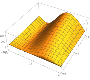
Figure 1: $u(x,0)=\sin(\pi x)$, with $\alpha=0.2$.

Figure 2: $u(x,0)=\sin(\pi x)$, with $\alpha=1$.

Example 3: Consider the Example 2 with the initial condition given by $u(x,0)=g(x)={\displaystyle{\frac{e^{x}}{1+e^{x}}}}$. Using Eq.(25) with $\lambda(t,\tau)=-1$ we get

$${u_{0}(x,t)=\frac{e^{x}}{1+e^{x}}},$$

$${\displaystyle{u_{1}(x,t)=\frac{e^{x}}{1+e^{x}}-\left(\frac{e^{x}(e^{x}+e^{2x}-1)}{(1+e^{x})^{3}}\right)\left(\frac{t^{\alpha}}{\Gamma(\alpha+1)}\right)}},$$

$${\displaystyle{u_{2}(x,t)=\frac{e^{x}}{1+e^{x}}-\left(\frac{e^{x}(e^{x}+e^{2x}-1)}{(1+e^{x})^{3}}\right)\left(\frac{t^{\alpha}}{\Gamma(\alpha+1)}\right)}}$$

$$\qquad\qquad\qquad+\left(\displaystyle{\frac{e^{x}(1-12e^{x}-29e^{2x}+4e^{3x}+37e^{4x}+50e^{5x}+11e^{6x}+2e^{7x})}{(1+e^{x})^{8}}}\right)$$

$$\qquad\qquad\qquad\qquad\times\left(\frac{t^{\alpha}}{\Gamma(1+2\alpha)}\right)-\left(\displaystyle{\frac{e^{x}(1-4e^{x}-10e^{2x}+6e^{3x}+2e^{4x}+e^{5x})}{(1+e^{x})^{6}}}\right)$$

$$\qquad\qquad\qquad\qquad\qquad\qquad\qquad\qquad\qquad\qquad\qquad\quad\times\left(\displaystyle{\frac{\Gamma(1+2\alpha)}{\Gamma^{2}(1+\alpha)}\frac{t^{3\alpha}}{\Gamma(1+3\alpha)}}\right).$$

Also here, the graphics in Figure 3, with $\alpha=0.2$ and Figure 4, with $\alpha=1$, elucidate the approximation of $u(x,t)$.

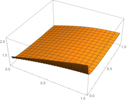
Figure 3: $u(x,0)=\displaystyle\frac{e^{x}}{1+e^{x}}$, with $\alpha=0.2$.

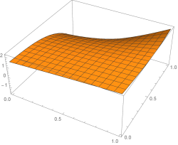
Figure 4: $u(x,0)=\displaystyle\frac{e^{x}}{1+e^{x}}$, with $\alpha=1$.

Example 4: Consider the problem

$$\left\{\begin{array}[]{l}{}_{c}{\sf D}_{t}^{\alpha}u+u\frac{\partial u}{\partial x}-\frac{\partial^{2}u}{\partial x^{2}}=0,\quad t>0,\quad 1<\alpha\leq 2,\\ \\ \displaystyle u(x,0)=\sin(\pi x),\qquad u_{t}(x,0)=0,\quad 0\leq x\leq 1.\end{array}\right.$$

In this case, using Eq.(25) with $\lambda(t,\tau)=\tau-t$ we obtain

$$\noindent{\displaystyle{u_{0}(x,t)=\sin(\pi x)}},$$

$$\noindent{\displaystyle{u_{1}(x,t)=\sin(\pi x)-\alpha(\alpha-1)[\pi\sin(\pi x)\cos(\pi x)-\pi^{2}\sin(x)]\left[\frac{t^{\alpha}}{\Gamma(\alpha+1)}\right]}},\noindent$$

$${\displaystyle{u_{2}(x,t)=\sin(\pi x)-\alpha(\alpha-1)[\pi\sin(\pi x)\cos(\pi x)-\pi^{2}\sin(x)]\left[\frac{t^{\alpha}}{\Gamma(\alpha+1)}\right]}}$$

$$\qquad\qquad+\alpha(\alpha-1)[\sin(\pi x)(2\pi^{2}\cos^{2}(\pi x)-\pi^{2}\sin^{3}(\pi x)+6\pi^{3}\cos(\pi x)$$

$$\qquad\qquad\qquad+\pi^{4}\sin^{3}(\pi x)]\left[\frac{t^{2}\alpha}{\Gamma(1+2\alpha)}\right]-\alpha(\alpha-1)(\pi\sin(\pi x))(\cos(\pi x)+x^{2})$$

$$\qquad\qquad\qquad\quad\times(\pi^{2}\cos(\pi x)-\pi^{2}\sin^{3}(\pi x)-\pi^{4}\sin(\pi x)\left[\frac{\Gamma(1+2\alpha)t^{3}\alpha}{\Gamma^{2}(1+\alpha)\Gamma(1+3\alpha)}\right].$$

The graphics in Figure 5, with $\alpha=1.2$ and Figure 6, with $\alpha=2$ one can see the evolution of the approximation of $u(x,t)$.

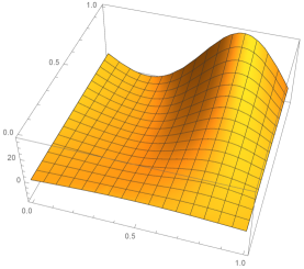
Figure 5: $u(x,0)=\sin(\pi x),u_{t}(x,0)=0$, with $\alpha=1.2$.

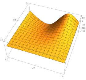
Figure 6: $u(x,0)=\sin(\pi x),u_{t}(x,0)=0$, with $\alpha=2$.

5 Conclusions

The FC is very useful in the recuperation of the memory of phenomena, by used of fractional derivative in time variable. News Lagrange multipliers for FPBE are identified by Laplace transform and particular cases are recovered. Using this multipliers and the VIM we obtained approximations of the solutions for FPBE taking three terms only. Then, we conclude that the VIM is a powerful and efficient technical to approximate solutions to FPBE.

References

References

• [1] I. Podlubny. Fractional differential equations, Academic Press, San Diego, 1999.
• [2] R. Gorenflo and F. Mainardi. Fractional calculus: integral and differential equations of fractional order. In: A. Carpinteri and F. Mainardi (editors): Fractals and Fractional Calculus in Continuum Mechanics. Springer Verlag, Wien and New York, 1997, pp. 223- 276.
• [3] L. Debnath, and D. Bhatta. Integral Transforms and their Applications, Chapman Hall / CRC, Boca Raton, London and New York. 2006.
• [4] E. Yusufoglu. Variational iteration method for construction of some compact and noncompact structures of Klein-Gordon equations, Int. J. Nonlinear. Sci. Numer. Simul., 8(2) (2007) 153-185.
• [5] C. P. Li and Y. H.Wang. Numerical algorithm based on Adomian decomposition for fractional differential equations. Comput. Math. Appl., 57 (2009) 1672-1681.
• [6] Z. Odibat. Reliable approaches of variational iteration method for nonlinear operators, Math. Comput. Model, 48 (2008) 895-902.
• [7] G-C Wu, and D. Baleanu. Variational iteration method for Burgers’ flow with fractional derivatives- New Lagrange multipliers. App. Math. Mod., 37 (2013) 6183-6190.
• [8] S. Momani, and Z.Odibat. Analytical approach to linear fractional partial differential equations arising in fluid mechanics. Phys Lett. A, 355 (2006) 271-279.
• [9] K. Diethelm. The Analysis of Fractional Differential Equations: An Application- Oriented Exposition using Differential Operator of Caputo Type, Springer, Braunschweig, 2010.
• [10] F. Mainardi, Y. Luchko, and G. Pagnini. The fundamental solution of the space-time fractional diffusion equation. Frac. Calc. Appl. Anal., 4 (2001) 153-192.
• [11] F. S. Costa, J. A. P. F. Marao, J. C. A. Soares, and E. Capelas de Oliveira. Similarity solution to fractional nonlinear space-time, diffusion-wave equation. J. Math. Phys, 56 (2015) 033507.
• [12] E. Capelas de Oliveira, F. Mainardi, and J. Vaz Jr. Fractional models of anomalous relaxation based on the Kilbas and Saigo function. Meccanica (Milano. Print), 49 (2014) 2049-2060.
• [13] R. Figuereido Camargo, E. Capelas de Oliveira, and J. Vaz, Jr. On anamalous diffusion and the fractional generalized Langevin equation for a harmonic oscillator. J. Math. Phys. 50 (2009) 123-518.
• [14] K. Diethelm, and N. J. Ford. Multi-order fractional differential equations and their numerical solution. Appl. Math. Comput, 154 (2004) 621-640.
• [15] F. W. Liu, and V. Anh, I. Turner. Numerical solution of the space fractional Fokker-Planck equation. J. Comput. Appl. Math., 166 (2004) 209-219.
• [16] A. M. Wazwaz. The variational iteration method for solving linear and nonlinear systems of PDEs. Comput. Math. Appl, 54 (2007) 895-902.
• [17] J. H. He. Approximate analytical solution for seepage flow with fractional derivatives in porous media. Comput. Methods Appl. Mech. Engrg., 167 (1998) 57-68.
• [18] J. H. He. Variational iteration method-Some recent results and new interpretations. J. Comput. Appl, Math., 1 (2007) 3-17.
• [19] J. H. He, and X. H. Wu. Variational iteration Method: New development and applications. Comput. Math. Appl., 54 (2007) 881-894.
• [20] F. Mainardi. Fractional relaxation-oscillation and fractional diffusion-wave phenomena, Chaos Solitons Fractals, 7 (1996) 1461-1477.
• [21] A. M. Wazwaz. The variational iteration method: A reliable analytic tool for solving linear and nonlinear wave equations. Comput. Math. Appl., 54 (2007) 926-932.
• [22] A. M. Wazwaz. The Variational iteration method: A powerful scheme for handling linear and nonlinear diffusion equations. Comput. Math. Appl., 54 (2007) 933-939.
• [23] H. Ozer. Application of the variational iteration method to the boundary value problems with jump discontinuities arising in solid mechanics. Int. J. Nonlinear Sci. Numer. Simul., 8 (2007) 513-518.
• [24] H. Sheng, and Y. Q. Chen. Application of numerical inverse Laplace transform algorithms in fractional calculus. J. Franklin Ins., 348 (2011) 315-330.
• [25] M. D. Ruiz-Medina, J. M. Angulo, and V. V. Anh. Scaling limit solution of a fractional Burgers’ equation, Stochastic Process. Appl., 93 (2001) 285-300.
• [26] T. Hayat, M. Khan, and S. Asghar. On the MHD flow of fractional generalized Burgers’ fluid with modified Darcy’s law, Acta. Mech. Sin., 23 (2007) 257-261.
• [27] S. H. A. M. Shah. Some helical flows of a Burgers’ fluid with fractional derivative. Meccanica, 45 (2010) 143-151.
• [28] Y. Chen, and H. L. An. Numerical solutions of coupled Burgers’ equations with time and space-fractional derivatives. Appl. Math. Comput., 200 (2008) 87-95.
• [29] Y. J. Jun, J. A. Tenreiro Machado, and J. Hristov. Nonlinear dynamics for local fractional Burgers’ equation arising in fractal flow. Nonlinear Dyn., (2015),DOI 10.1007/s11071-015-2085-2.
• [30] Z. Odibat, and S. Momami. The variational iteration method: An efficient scheme for handling fractional partial differential equations in fluid mechanics. Comp. Math. Appl., 58 (2009) 2199-2208.
• [31] M. Inokuti, H. Sekine, and T. Mura. General use of the Lagrange multiplier in non-linear mathematical physics, in: S Nemat-Nasser (Ed), Variational Method in the Mechanics of Solid, Pergamon Press, Oxford, (1978) 156-162.
• [32] W. Deng. Short memory principle and a predictor-corrector approach for fractional differential equations. J. Comput. Appl. Math., 206 (2007) 174-188.