The Lyapunov dimension formula for
the global attractor of the Lorenz system

Abstract

The exact Lyapunov dimension formula for the Lorenz system has been analytically obtained first due to G.A.Leonov in 2002 under certain restrictions on parameters, permitting classical values. He used the construction technique of special Lyapunov-type functions developed by him in 1991 year. Later it was shown that the consideration of larger class of Lyapunov-type functions permits proving the validity of this formula for all parameters of the system such that all the equilibria of the system are hyperbolically unstable. In the present work it is proved the validity of the formula for Lyapunov dimension for a wider variety of parameters values, which include all parameters satisfying the classical physical limitations. One of the motivation of this work is the possibility of computing a chaotic attractor in the Lorenz system in the case of one unstable and two stable equilibria.

1 Introduction

The exact Lyapunov dimension formula for the Lorenz system has been analytically obtained first due to G.A.Leonov in 2002 [1] under certain restrictions on parameters, permitting classical values. In his work it was used the technique of special Lyapunov-type functions, which had been created in 1991 year [2] and then was developed in [3, 4]. Later in the works [5, 6, 7] it was shown that the consideration of a wider class of Lyapunov-type functions allows to provide the validity of the formula for such parameters of the Lorenz system that all its equilibria are hyperbolically unstable.

In this study it is proved the validity of the formula under classical restrictions on the parameters. The motivation for this investigation is a numerical localization of chaotic attractor in the Lorenz system in the case of one unstable and two stable equilibria [8, 9].

2 The Lorenz system

Consider the classical Lorenz system suggested in the original work of Edward Lorenz [10]:

$$\left\{\begin{aligned} &\dot{x}=\sigma(y-x)\\ &\dot{y}=rx-y-xz\\ &\dot{z}=-bz+xy.\end{aligned}\right.$$ (1)

E. Lorenz obtained his system as a truncated model of thermal convection in a fluid layer. The parameters of this system are positive:

$$\sigma>0,\ \rho>0,\ b>0,$$

because of their physical meaning (e.g., $b=4(1+a^{2})^{-1}$ is positive and bounded).

Active study of the Lorenz system gave rise to the appearance and subsequent consideration of various Lorenz-like systems (see, e.g., [11, 12, 13, 14]). A recent discussion of the equivalence of some Lorenz-like systems and the possibility of universal consideration of their behavior can be found, e.g. in [15, 16].

Since the system is dissipative and generates a dynamical system for $\forall t\geq 0$ (to verify this, it suffices to consider the Lyapunov function $V(x,y,z)=\frac{1}{2}(x^{2}+y^{2}+(z-r-\sigma)^{2})$; see, e.g., [10, 4]), it possesses a global attractor (a bounded closed invariant set, which is globally attractive) [17, 4].

For the Lorenz system, the following classical scenario of transition to chaos is known [8]. Suppose that $\sigma$ and $b$ are fixed (we use the classical parameters $\sigma=10$, $b=8/3$) and $r$ varies. Then, as $r$ increases, the phase space of the Lorenz system is subject to the following sequence of bifurcations. For $0<r<1$, there is globally asymptotically stable zero equilibrium $S_{0}$. For $r>1$, equilibrium $S_{0}$ is a saddle and a pair of symmetric equilibria $S_{1,2}$ appears. For $1<r<r_{h}\approx 13.9$, the separatrices $\Gamma_{1,2}$ of equilibria $S_{0}$ are attracted to the equilibria $S_{1,2}$. For $r=r_{h}\approx 13.9$, the separatrices $\Gamma_{1,2}$ form two homoclinic trajectories of equilibria $S_{0}$ (homoclinic butterfly). For $r_{h}<r<r_{c}\approx 24.06$, the separatrices $\Gamma_{1}$ and $\Gamma_{2}$ tend to $S_{2}$ and $S_{1}$, respectively. For $r_{c}<r<r_{a}\approx 24.74$, the equilibria $S_{1,2}$ are stable and the separatrices $\Gamma_{1,2}$ may be attracted to a local chaotic attractor (see, e.g., [8, 9]). This attractor is self-excited and can be found using the standard computational procedure, i.e. by constructing a solution using initial data from a small neighborhood of zero equilibrium, observing how it is attracted, and visualizing the attractor (see Fig 1).

(a)

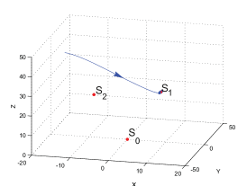
(b)

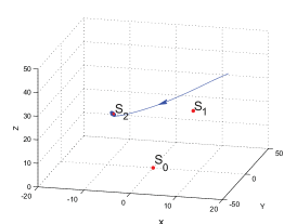
(c)

Figure 1: (a) Numerical visualization of a self-excited Lorenz attractor by using a trajectory with an initial point taken in the vicinity of the equilibrium $S_{0}$. (b), (c) Trajectories with the initial conditions $(\mp 16.2899,\,\mp 0.0601,\,42.1214)$ tend to equilibria $S_{2,1}$. Parameters: $r=24.5$, $\sigma=10$, $b=8/3$.

For $r>r_{a}$, the equilibria $S_{1,2}$ become unstable. The value $r=28$ corresponds to the classical self-excited local attractor (see Fig. 2).

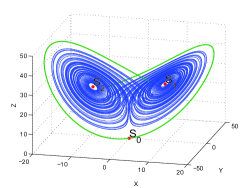
(a) Initial data near the equilibrium $S_{0}$

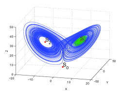
(b) Initial data near the equilibrium $S_{1}$

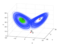
(c) Initial data near the equilibrium $S_{2}$

Figure 2: Numerical visualization of the classical self-excited local attractor in the Lorenz system by using the trajectories that start in small neighborhoods of the unstable equilibria $S_{0,1,2}$. Here the separation of the trajectory into transition process (green) and approximation of attractor (blue) is rough.

3 Lyapunov dimension of attractors

Consider a dynamical system

$$\dot{{\bf\rm x}}={\bf\rm f}({\bf\rm x}),$$ (2)

where ${\bf\rm f}:\mathbb{R}^{n}\to\mathbb{R}^{n}$ is a smooth vector-function. Since the initial time is not important for dynamical systems, without loss of generality, we consider a solution $x(t,x_{0}):\ x(0,x_{0})=x_{0}.$ The linearized system along the solution ${\bf\rm x}(t,{\bf\rm x}_{0})$ is as follows

$$\dot{{\bf\rm u}}=J({\bf\rm x}(t,{\bf\rm x}_{0}))\,{\bf\rm u},\quad{\bf\rm u}\in\mathbb{R}^{n},~{}t\in\mathbb{R}_{+},$$ (3)

where

$$J({\bf\rm x}(t,{\bf\rm x}_{0}))=\left[\frac{\partial f_{i}({\bf\rm x})}{\partial{\bf\rm x}_{j}}\big{|}_{{\bf\rm x}={\bf\rm x}(t,{\bf\rm x}_{0})}\right]$$

is the $(n\times n)$ Jacobian matrix evaluated along the trajectory ${{\bf\rm x}(t,{\bf\rm x}_{0})}$ of system (2). A fundamental matrix $X(t,{\bf\rm x}_{0})$ of linearized system (3) is defined by the variational equation

$$\dot{X}(t,{\bf\rm x}_{0})=J({\bf\rm x}(t,{\bf\rm x}_{0}))\,X(t,{\bf\rm x}_{0}).$$ (4)

We usually set $X(0,{\bf\rm x}_{0})=I_{n}$, where $I_{n}$ is the identity matrix. Then ${\bf\rm u}(t,{\bf\rm u}_{0})=X(t,{\bf\rm x}_{0}){\bf\rm u}_{0}$. In the general case, ${\bf\rm u}(t,{\bf\rm u}_{0})=X(t,{\bf\rm x}_{0})X^{-1}(0,{\bf\rm x}_{0}){\bf\rm u}_{0}$. Note that if a solution of nonlinear system (2) is known, then we have

$$X(t,{\bf\rm x}_{0})=\frac{\partial{\bf\rm x}(t,{\bf\rm x}_{0})}{\partial{\bf\rm x}_{0}}.$$

Consider the transformation of the unit ball $B$ into the ellipsoid $X(t,x_{0})B$ and the exponential growth rates of its principal semiaxes lengths. The principal semiaxes of the ellipsoid $X(t,x_{0})B$ coincides with singular values of the matrix $X(t,x_{0})$,which are defined as the square roots of the eigenvalues of matrix $X(t,x_{0})^{*}X(t,x_{0})$. Let $\sigma_{1}(X(t,{\bf\rm x}_{0}))\geq\cdots\geq\sigma_{n}(X(t,{\bf\rm x}_{0}))>0$ denote the singular values of the fundamental matrix $X(t,{\bf\rm x}_{0})$ reordered for each $t$. Introduce the operator $\mathcal{X}(\cdot)=\frac{1}{t}\ln|\cdot|$, where $|\cdot|$ is the Euclidian norm. Define the decreasing sequence (for all considered $t$) of Lyapunov exponents functions $\operatorname{LE}_{i}(t,x_{0})=\mathcal{X}({\sigma_{i}}(t,x_{0}))$

$$\operatorname{LE}_{1}(t,x_{0})\geq\operatorname{LE}_{2}(t,x_{0})\geq...\geq\operatorname{LE}_{n}(t,x_{0}).$$

Definition 1.

[37] The Lyapunov exponents (LEs) at the point ${\bf\rm x}_{0}$ are the numbers (or the symbols $\pm\infty$) defined as

$${\rm LE}_{i}({\bf\rm x}_{0})=\limsup_{t\to\infty}\operatorname{LE}_{i}(t,x_{0})=\limsup_{t\to\infty}\frac{1}{t}\ln\sigma_{i}(X(t,{\bf\rm x}_{0})).$$ (5)

LEs are commonly used in the theory of dynamical systems and dimension theory [46, 47, 48, 49, 50, 4, 51].

Remark 1.

The LEs are independent of the choice of fundamental matrix at the point ${\bf\rm x}_{0}$ [45, 52].

Consider the largest integer $j(t,x_{0})\in\{1,..,n\}$ such that

$$\begin{array}[]{c}\operatorname{LE}_{1}^{o}(t,x_{0})+\ldots+\operatorname{LE}_{j(t,x_{0})}^{o}(t,x_{0})>0,\\ \vskip 3.0pt plus 1.0pt minus 1.0pt\\ \cfrac{\operatorname{LE}_{1}^{o}(t,x_{0})+\ldots+\operatorname{LE}_{j(t,x_{0})}^{o}(t,x_{0})}{|\operatorname{LE}_{j(t,x_{0})+1}^{o}(t,x_{0})|}<1.\end{array}$$

Following [53, 49], introduce the following definition: the function $\operatorname{LD}(t,x_{0})=0$ if $\operatorname{LE}^{o}_{1}(t,x_{0})\leq 0$ and $\operatorname{LD}(t,x_{0})=n$ if $\sum_{i=1}^{n}\operatorname{LE}^{o}_{i}(t,x_{0})\geq 0$, otherwise

$$\operatorname{LD}(t,x_{0})=j(t,x_{0})+\cfrac{\operatorname{LE}_{1}^{o}(t,x_{0})+\ldots+\operatorname{LE}_{j(t,x_{0})}^{o}(t,x_{0})}{|\operatorname{LE}_{j(t,x_{0})+1}^{o}(t,x_{0})|}.$$ (6)

Definition 2.

A local Lyapunov dimension at the point $x_{0}$ is as follows

$$\operatorname{LD}(x_{0})=\limsup\limits_{t\to+\infty}\operatorname{LD}(t,x_{0}).$$

The Lyapunov dimension of invariant compact set $K$ of dynamical system is defined by the relation

$$\dim_{L}K=\sup\limits_{x_{0}\in K}\operatorname{LD}(x_{0})=\sup\limits_{x_{0}\in K}\limsup\limits_{t\to+\infty}\operatorname{LD}(t,x_{0})$$

.

Note that, from an applications perspective, an important property of the Lyapunov dimension is the chain of inequalities [49, 54, 4]

$$\dim_{T}K\leqslant\dim_{H}K\leqslant\dim_{F}K\leqslant\dim_{L}K,$$ (7)

where $\dim_{T}$, $\dim_{H}K,$ and $\dim_{F}K$ are topological, Hausdorff, and fractal dimensions of $K$, respectively.

4 Estimation of Lyapunov dimension by Lyapunov functions

Along with commonly used numerical methods for estimating and computing the Lyapunov dimension (see, e.g., [44, 24]), there is an analytical approach that was proposed by G.A.Leonov [2, 3, 4, 55, 5, 15]. It is based on the direct Lyapunov method and uses Lyapunov-like functions. The advantage of this method is that it allows to estimate the Lyapunov dimension of invariant set without numerical localization of the set. This is especially important for the systems with hidden attractors when numerical finding of all local attractors may be a challenging task [24].

Since LEs and LD are invariant under the linear changes of variables (see, e.g., [45]), we can apply the linear variable change ${\bf\rm y}=S{\bf\rm x}$ with a nonsingular $n\times n$-matrix $S$. Then system (2) is transformed into the system

$$\dot{{\bf\rm y}}=S\,\dot{{\bf\rm x}}=S\,{\bf\rm f}(S^{-1}{\bf\rm y})=\tilde{{\bf\rm f}}({\bf\rm y}).$$

Consider the linearization along the corresponding solution ${\bf\rm y}(t,{\bf\rm y}_{0})=S{\bf\rm x}(t,S^{-1}{\bf\rm x}_{0})$, that is,

$$\dot{\bf\rm v}=\tilde{J}({\bf\rm y}(t,{\bf\rm y}_{0}))\,{\bf\rm v},\quad{\bf\rm v}\in\mathbb{R}^{n}.$$ (8)

Here the Jacobian matrix is as follows

$$\tilde{J}({\bf\rm y}(t,{\bf\rm y}_{0}))=S\,J({\bf\rm x}(t,{\bf\rm x}_{0}))\,S^{-1}$$ (9)

and the corresponding fundamental matrix satisfies $Y(t,{\bf\rm y}_{0})=SX(t,{\bf\rm x}_{0}).$

For simplicity, let $J({\bf\rm x})=J({\bf\rm x}(t,{\bf\rm x}_{0}))$. Suppose that

$\lambda_{1}({\bf\rm x},S)\geqslant\cdots\geqslant\lambda_{n}({\bf\rm x},S)$ are eigenvalues of the symmetrized Jacobian matrix (9)

$$\frac{1}{2}\left(SJ({\bf\rm x})S^{-1}+(SJ({\bf\rm x})S^{-1})^{*}\right).$$ (10)

Theorem 1 ([5]).

Given an integer $j\in[1,n]$ and $s\in[0,1]$, suppose that there are a continuously differentiable scalar function $\vartheta:\mathbb{R}^{n}\rightarrow\mathbb{R}$ and a nonsingular matrix $S$ such that

$$\lambda_{1}({\bf\rm x},S)+\cdots+\lambda_{j}({\bf\rm x},S)+s\lambda_{j+1}({\bf\rm x},S)+\dot{\vartheta}({\bf\rm x})<0,~{}\forall\,{\bf\rm x}\in K.$$ (11)

Then $\dim_{L}K\leqslant j+s$.

Here $\dot{\vartheta}$ is the derivative of $\vartheta$ with respect to the vector field ${\bf\rm f}$:

$$\dot{\vartheta}({\bf\rm x})=({\rm grad}(\vartheta))^{*}{\bf\rm f}({\bf\rm x}).$$

Theorem 2 ([2, 3, 4, 5]).

Assume that there are a continuously differentiable scalar function $\vartheta$ and a nonsingular matrix $S$ such that

$$\lambda_{1}({\bf\rm x},S)+\lambda_{2}({\bf\rm x},S)+\dot{\vartheta}({\bf\rm x})<0,~{}\forall\,{\bf\rm x}\in\mathbb{R}^{n}.$$ (12)

Then any solution of system (2) bounded on $[0,+\infty)$ tends to a certain equilibrium as $t\rightarrow+\infty$.

5 Main result: Lyapunov dimension of the global Lorenz attractor

By Theorems 1 and 2, for the Lorenz system we can obtain the following result.

Theorem 3.

Assume that the following inequalities

$$r-1>0,$$ (13)

$$r-1\geq\frac{b(b+\sigma-1)^{2}-4\sigma(b+\sigma b-b^{2})}{3\sigma^{2}}$$ (14)

are satisfied. Let one of the following two conditions be satisfied:

• $$\sigma^{2}(r-1)(b-4)\leq 4\sigma(\sigma b+b-b^{2})-b(b+\sigma-1)^{2};$$ (15)

• there are two distinct real roots of equations

  $$\begin{split}(2\sigma-b+\gamma)^{2}\left(b(b+\sigma-1)^{2}-4\sigma(\sigma b+b-b^{2})+\sigma^{2}(r-1)(b-4)\right)+\\ +4b\gamma(\sigma+1)\left(b(b+\sigma-1)^{2}-4\sigma(\sigma b+b-b^{2})-3\sigma^{2}(r-1)\right)=0\end{split}$$ (16)

  and

  $$\left\{\begin{gathered}\sigma^{2}(r-1)(b-4)>4\sigma(\sigma b+b-b^{2})-b(b+\sigma-1)^{2}\hfill\\ \gamma^{(II)}>0\hfill\\ \end{gathered}\right.\hfill\\$$ (17)

  where $\gamma^{(II)}$ is a greater root of equation (16).

In this case

1. if

   $$(b-\sigma)(b-1)<\sigma r<(b+1)(b+\sigma),$$ (18)

   then any bounded on $[0;+\infty)$ solution of system (1) tends to a certain equilibrium as $t\to+\infty$.

2. If

   $$\sigma r>(b+1)(b+\sigma),$$ (19)

   then

   $$\dim_{L}K\leq 3-\frac{2(\sigma+b+1)}{\sigma+1+\sqrt{(\sigma-1)^{2}+4\sigma r}},$$ (20)

where $K$ is a bounded invariant set.

For numerical experiments (see, e.g., [56, 57]) it is known that the Lyapunov dimension of any invariant compact set of the Lorenz system is bounded from above by the local Lyapunov dimension of the zero equilibrium.

Lemma 1.

If for the parameters of system (1) inequality (19) is valid, then

$$\dim_{L}(0,0,0)=3-\frac{2(\sigma+b+1)}{\sigma+1+\sqrt{(\sigma-1)^{2}+4r\sigma}}.$$

Comparing estimation (20) with the local dimension in the origin, we obtain a dimension formula for a global Lorenz attractor.

Theorem 4.

Let $K$ be a global attractor of classical Lorenz system (1) and conditions (13)-(17) of Theorem 3 be hold true.

In this case if

$$\sigma r>(b+1)(b+\sigma),$$

then

$$\dim_{L}K=3-\frac{2(\sigma+b+1)}{\sigma+1+\sqrt{(\sigma-1)^{2}+4\sigma r}}.$$ (21)

Remark 2.

It can be easily checked numerically that if all three equilibria are hyperbolic, then the conditions of Theorem 4 (see Fig. 3b) are satisfied. For example, for the standard parameters $\sigma=10$ and $b=\frac{8}{3}$ the formula (21) is valid for $r>\frac{209}{45}$.

(a) $r=10$

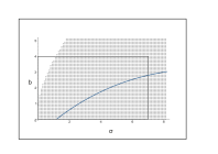
(b) $r=28$

(c) $r=100$

Figure 3: Numerical simulation of domains for the fixed values of parameter $r=10,28,100$

5.1 Numerical analysis

We perform a numerical analysis of parameter domain, which does not satisfy the conditions of Theorem 4.

1. Recall that for $0<r<1$ the solutions of system tend to a unique equilibria (see., e.g., [4]).

2. Consider $r>1$. In the case of conditions (13)-(19) the following assertion is valid.

Lemma 2.

For all $r>1$, $\sigma>7$, and $0<b<4$ the conditions of Theorem 3 are satisfied.

Remark 3.

For $0<b<4-\epsilon$, $\sigma>7$ and $r>r_{*}$, where $r_{*}=r_{*}(\epsilon)$, the conditions of Theorem 3 are satisfied.

Thus, for each fixed $r>1$ it remains to check numerically the behavior of system with the parameters from the bounded domain $[0<b<4,0<\sigma<7]$. For the considered increasing sequence $r_{k}>1$, numerical simulation shows the lack of chaotic attractor (the trajectories with initial data from the corresponding compact absorbing set [58] have been simulated).

Appendix

Proof.

(Theorem 1)

For the proof we make use of Theorems 1, 2. Consider a solution of system (1) ${\bf\rm x}=(x(t),y(t),z(t))=(x,y,z)$.

I. In the case of classical Lorenz system the matrix $J$ has the following form

$$J=\begin{pmatrix}-\sigma&\sigma&0\\ r-z&-1&-x\\ y&x&-b\end{pmatrix}$$

Following [4], for the condition

$$\sigma r+(\sigma-b)(b-1)>0$$ (22)

we introduce a matrix

$$S=\begin{pmatrix}-\rho^{-1}&0&0\\ -\frac{b-1}{\sigma}&1&0\\ 0&0&1\end{pmatrix},$$

where

$$\rho=\frac{\sigma}{\sqrt{\sigma r+(\sigma-b)(b-1)}}.$$ (23)

Then

$$SJS^{-1}=\begin{pmatrix}b-\sigma-1&-\frac{\sigma}{\rho}&0\\ -\frac{\sigma}{\rho}+\rho z&-b&-x\\ -\rho\left(y+\frac{b-1}{\sigma}x\right)&x&-b\end{pmatrix}.$$

We find the eigenvalues of the matrix $\frac{1}{2}(SJS^{-1}+(SJS^{-1})^{*})$. The characteristic polynomial of the matrix takes the form:

$$(\lambda+b)\left[\lambda^{2}+(\sigma+1)\lambda+b(\sigma-b+1)-\left(\frac{\sigma}{\rho}-\frac{\rho z}{2}\right)^{2}-\left(\frac{\rho(b-1)}{2\sigma}x+\frac{\rho}{2}y\right)^{2}\right].$$

This implies that the eigenvalues $\lambda_{i}=\lambda_{i}(x,y,z,S),i=1,2,3$ of the matrix $\frac{1}{2}(SJS^{-1}+(SJS^{-1})^{*})$ are the numbers:

$$\lambda_{2}=-b,$$

$$\lambda_{1,3}=-\frac{\sigma+1}{2}\pm\frac{1}{2}\left[(\sigma-2b+1)^{2}+\left(\frac{2\sigma}{\rho}-\rho z\right)^{2}+\rho^{2}\left(y+\frac{b-1}{\sigma}x\right)^{2}\right]^{\frac{1}{2}}.$$

Such a choice of the matrix $S$ provides a simple form of eigenvalues.

II. We shall show that $\lambda_{1}\geq\lambda_{2}\geq\lambda_{3},\forall x,y,z$:

$$\frac{-(\sigma+1)+\sqrt{(\sigma-2b+1)^{2}+\left(\frac{2\sigma}{\rho}-\rho z\right)^{2}+\rho^{2}\left(y+\frac{b-1}{\sigma}x\right)^{2}}}{2}\geq-b\geq$$

$$\geq\frac{-(\sigma+1)-\sqrt{(\sigma-2b+1)^{2}+\left(\frac{2\sigma}{\rho}-\rho z\right)^{2}+\rho^{2}\left(y+\frac{b-1}{\sigma}x\right)^{2}}}{2}$$

$$\Leftrightarrow$$

$$\sqrt{(\sigma-2b+1)^{2}+\left(\frac{2\sigma}{\rho}-\rho z\right)^{2}+\rho^{2}\left(y+\frac{b-1}{\sigma}x\right)^{2}}\geq\sigma-2b+1\geq$$

$$\geq-\sqrt{(\sigma-2b+1)^{2}+\left(\frac{2\sigma}{\rho}-\rho z\right)^{2}+\rho^{2}\left(y+\frac{b-1}{\sigma}x\right)^{2}}$$

$$\Leftrightarrow$$

$$\sqrt{(\sigma-2b+1)^{2}+\left(\frac{2\sigma}{\rho}-\rho z\right)^{2}+\rho^{2}\left(y+\frac{b-1}{\sigma}x\right)^{2}}\geq|\sigma-2b+1|$$

$$\left(\frac{2\sigma}{\rho}-\rho z\right)^{2}+\rho^{2}\left(y+\frac{b-1}{\sigma}x\right)^{2}\geq 0.$$

At the left there is a sum of two total squares, i.e. the inequality is always satisfied.

Thus, $\lambda_{1}\geq\lambda_{2}\geq\lambda_{3},\forall x,y,z$.

III. To apply Theorem 1 and Theorem 2, for $s\in[0,1)$, we consider and transform the relation $2(\lambda_{1}+\lambda_{2}+s\lambda_{3})$:

$$\begin{split}&2(\lambda_{1}+\lambda_{2}+s\lambda_{3})=-(\sigma+2b+1)-s(\sigma+1)+\\ &+(1-s)\left[(\sigma-2b+1)^{2}+\left(\frac{2\sigma}{\rho}-\rho z\right)^{2}+\rho^{2}\left(y+\frac{b-1}{\sigma}x\right)^{2}\right]^{\frac{1}{2}}=\\ &-(\sigma+2b+1)-s(\sigma+1)+\\ &+(1-s)\left[(\sigma-2b+1)^{2}+\frac{4\sigma^{2}}{\rho^{2}}-4\sigma z+\rho^{2}z^{2}+\rho^{2}\left(y+\frac{b-1}{\sigma}x\right)^{2}\right]^{\frac{1}{2}}=\\ &=-(\sigma+2b+1)-s(\sigma+1)+\\ &+(1-s)\left[(\sigma-1)^{2}+4\sigma r-4\sigma z+\rho^{2}z^{2}+\rho^{2}\left(y+\frac{b-1}{\sigma}x\right)^{2}\right]^{\frac{1}{2}}.\end{split}$$ (24)

We can use the inequality

$$\sqrt{k+l}\leq\sqrt{k}+\frac{l}{2\sqrt{k}}$$ (25)

for $k+l>0,k>0$. Consider

$$k+l=(\sigma-1)^{2}+4\sigma r-4\sigma z+\rho^{2}z^{2}+\rho^{2}\left(y+\frac{b-1}{\sigma}x\right)^{2}$$

and

$$k=(\sigma-1)^{2}+4\sigma r.$$

According to (24) the following equation

$$\begin{split}&k+l=(\sigma-1)^{2}+4\sigma r-4\sigma z+\rho^{2}z^{2}+\rho^{2}\left(y+\frac{b-1}{\sigma}x\right)^{2}=\\ &=(\sigma-2b+1)^{2}+\left(\frac{2\sigma}{\rho}-\rho z\right)^{2}+\rho^{2}\left(y+\frac{b-1}{\sigma}x\right)^{2}\geq 0\end{split}$$

is valid. By the condition of Theorem 3 we have

$$r\sigma+(\sigma-b)(b-1)>0\Leftrightarrow r\sigma>-\sigma b+\sigma+b^{2}-b.$$

Then

$$k=(\sigma-1)^{2}+4\sigma r>(\sigma-1)^{2}-4\sigma b+4\sigma+4b^{2}-4b=(\sigma-2b+1)^{2}\geq 0.$$

Applying the inequality (25) with $k=(\sigma-1)^{2}+4\sigma r$ and $l=-4\sigma z+\rho^{2}z^{2}+\rho^{2}\left(y+\frac{b-1}{\sigma}x\right)^{2}$ to the relation (24), we obtain

$$\begin{split}&2(\lambda_{1}+\lambda_{2}+s\lambda_{3})\leq-(\sigma+2b+1)-s(\sigma+1)+(1-s)[(\sigma-1)^{2}+4\sigma r]^{\frac{1}{2}}+\\ &+\frac{2(1-s)}{[(\sigma-1)^{2}+4\sigma r]^{\frac{1}{2}}}\left[-\sigma z+\frac{\rho^{2}z^{2}}{4}+\frac{\rho^{2}}{4}\left(y+\frac{b-1}{\sigma}x\right)^{2}\right].\end{split}$$ (26)

Introduce the function

$$\theta(x,y,z)=\frac{(1-s)V(x,y,z)}{[(\sigma-1)^{2}+4\sigma r]^{\frac{1}{2}}},$$ (27)

where

$$V(x,y,z)=\gamma_{4}x^{2}+(-\sigma\gamma_{1}+\gamma_{3})y^{2}+\gamma_{3}z^{2}+\frac{1}{4\sigma}\gamma_{1}x^{4}-\gamma_{1}x^{2}z-\gamma_{1}\gamma_{2}xy-\frac{\sigma}{b}z.$$ (28)

We choose the running parameters $\gamma_{1},\gamma_{2},\gamma_{3},\gamma_{4}$ in such a way that

$$R:=-\sigma z+\frac{\rho^{2}z^{2}}{4}+\frac{\rho^{2}}{4}\left(y+\frac{b-1}{\sigma}x\right)^{2}+\dot{V}\leq 0\quad\forall x,y,z,$$ (29)

where $\dot{V}(x)$ is a derivative with respect to system (1). Then, using (26), we obtain

$$2(\lambda_{1}+\lambda_{2}+s\lambda_{3})+2\dot{\theta}\leq-(\sigma+2b+1)-s(\sigma+1)+(1-s)[(\sigma-1)^{2}+4\sigma r]^{\frac{1}{2}},$$ (30)

i.e. we estimated $2(\lambda_{1}+\lambda_{2}+s\lambda_{3})+2\dot{\theta}$ by the relation, which depends on the parameters of system (1) and is independent of $x,y,z$.

IV. We perform the analysis of $R$, choosing the running parameters $\gamma_{1},\gamma_{2},\gamma_{3},\gamma_{4}$ in such a way that (29) is valid. Taking into account (28), we obtain

$$R=-\gamma_{1}x^{4}+(\gamma_{1}\gamma_{2}+2\sigma\gamma_{1}+b\gamma_{1})x^{2}z+\left(\frac{\rho^{2}(b-1)^{2}}{4\sigma^{2}}-r\gamma_{1}\gamma_{2}-2\sigma\gamma_{4}\right)x^{2}+$$

$$+\left(\frac{\rho^{2}(b-1)}{2\sigma}+\gamma_{1}\gamma_{2}-2r\sigma\gamma_{1}+2r\gamma_{3}+2\sigma\gamma_{4}+\sigma\gamma_{1}\gamma_{2}-\frac{\sigma}{b}\right)xy+$$

$$+\left(2\sigma\gamma_{1}-2\gamma_{3}-\sigma\gamma_{1}\gamma_{2}+\frac{\rho^{2}}{4}\right)y^{2}+\left(\frac{\rho^{2}}{4}-2b\gamma_{3}\right)z^{2}=$$

$$=A_{1}x^{4}+A_{2}x^{2}z+A_{3}z^{2}+B_{1}x^{2}+B_{2}xy+B_{3}y^{2},$$

where

$$A_{1}=-\gamma_{1},A_{2}=\gamma_{1}(\gamma_{2}+2\sigma+b),A_{3}=\frac{\rho^{2}}{4}-2b\gamma_{3}$$

$$B_{1}=\frac{\rho^{2}(b-1)^{2}}{4\sigma^{2}}-r\gamma_{1}\gamma_{2}-2\sigma\gamma_{4}=C_{1}-2\sigma\gamma_{4}$$

$$B_{2}=\frac{\rho^{2}(b-1)}{2\sigma}+\gamma_{1}\gamma_{2}-2r\sigma\gamma_{1}+2r\gamma_{3}+\sigma\gamma_{1}\gamma_{2}-\frac{\sigma}{b}+2\sigma\gamma_{4}=C_{2}+2\sigma\gamma_{4}$$

$$B_{3}=2\sigma\gamma_{1}-2\gamma_{3}-\sigma\gamma_{1}\gamma_{2}+\frac{\rho^{2}}{4}.$$

IV. a. Under the conditions $A_{1}\neq 0$ and $B_{3}\neq 0$ we transform the relation for $R$:

$$R=A_{1}\left(x^{2}+\frac{A_{2}}{2A_{1}}z\right)^{2}+B_{3}\left(y+\frac{B_{2}}{2B_{3}}x\right)^{2}+\frac{4B_{1}B_{3}-B_{2}^{2}}{4B_{3}}x^{2}+\frac{4A_{1}A_{3}-A_{2}^{2}}{4A_{1}}z^{2}$$ (31)

Then

$$\left.\begin{aligned} &A_{1}<0\\ &B_{3}<0\\ &4A_{1}A_{3}-A_{2}^{2}\geq 0\\ &4B_{1}B_{3}-B_{2}^{2}\geq 0\end{aligned}\right\}\Rightarrow R\leq 0\quad\forall x,y,z$$ (32)

Now we analyze the signs of four addends in (31)

(1)

$$A_{1}=-\gamma_{1}<0\Leftrightarrow\gamma_{1}>0$$ (33)

(2)

$$B_{3}<0\Leftrightarrow 2\gamma_{3}>2\sigma\gamma_{1}-\sigma\gamma_{1}\gamma_{2}+\frac{\rho^{2}}{4}$$ (34)

(3)

$$0\leq 4A_{1}A_{3}-A_{2}^{2}=-4\gamma_{1}\left(\frac{\rho^{2}}{4}-2b\gamma_{3}\right)-{\gamma_{1}}^{2}(\gamma_{2}+2\sigma+b)^{2}.$$ (35)

Since according to (33), $\gamma_{1}>0$, from (35) it follows that

$$-\gamma_{1}(\gamma_{2}+2\sigma+b)^{2}-\rho^{2}+8b\gamma_{3}\geq 0$$

$$\Leftrightarrow$$

$$2\gamma_{3}\geq\frac{\rho^{2}}{4b}+\frac{\gamma_{1}}{4b}(\gamma_{2}+2\sigma+b)^{2}.$$ (36)

(4)

$$4B_{1}B_{3}-B_{2}^{2}=4B_{3}(C_{1}-2\sigma\gamma_{4})-(C_{2}+2\sigma\gamma_{4})^{2}=$$

$$=4B_{3}C_{1}-8\sigma B_{3}\gamma_{4}-C_{2}^{2}-4\sigma C_{2}\gamma_{4}-4\sigma^{2}\gamma_{4}^{2}=$$

$$=-4\sigma^{2}\gamma_{4}^{2}+4\gamma_{4}\sigma(-2B_{3}-C_{2})+4B_{3}C_{1}-C_{2}^{2}.$$

The relation $4B_{1}B_{3}-B_{2}^{2}$ is a quadratic polynomial in $\gamma_{4}$ with a negative coefficient of $\gamma_{4}^{2}$. Therefore for the inequality $4B_{1}B_{3}-B_{2}^{2}\geq 0$ to be satisfied, it is necessary that the corresponding quadratic equation has a real root, i.e. a positive discriminant:

$$D_{\gamma_{4}}=16\sigma^{2}(4B_{3}^{2}+C_{2}^{2}+4B_{3}C_{2})+16\sigma^{2}(4B_{3}C_{1}-C_{2}^{2})=$$

$$=16C_{2}^{2}\sigma^{2}+64\sigma^{2}B_{3}^{2}+64\sigma^{2}B_{3}C_{2}+64\sigma^{2}B_{3}C_{1}-16\sigma^{2}C_{2}^{2}=64\sigma^{2}B_{3}(B_{3}+C_{2}+C_{1}).$$

Since according to (32) the condition $B_{3}<0$ is satisfied, we obtain $D_{\gamma_{4}}\geq 0\Leftrightarrow B_{3}+C_{1}+C_{2}\leq 0$. We have

$$B_{3}+C_{1}+C_{2}=2\sigma\gamma_{1}-2\gamma_{3}-\sigma\gamma_{1}\gamma_{2}+\frac{\rho^{2}}{4}+\frac{\rho^{2}(b-1)^{2}}{4\sigma^{2}}+$$

$$-r\gamma_{1}\gamma_{2}+\frac{\rho^{2}(b-1)}{2\sigma}+\gamma_{1}\gamma_{2}-2r\sigma\gamma_{1}+2r\gamma_{3}+\sigma\gamma_{1}\gamma_{2}-\frac{\sigma}{b}=$$

$$=\gamma_{3}(2r-2)-\gamma_{1}(-2\sigma+2r\sigma)-\gamma_{1}\gamma_{2}(\sigma+r-\sigma-1)+\frac{\rho^{2}}{4}+\frac{\rho^{2}(b-1)^{2}}{4\sigma^{2}}+$$

$$+\frac{\rho^{2}(b-1)}{2\sigma}-\frac{\sigma}{b}=2\gamma_{3}(r-1)-2\sigma\gamma_{1}(r-1)-\gamma_{1}\gamma_{2}(r-1)+\frac{\rho^{2}}{4}+$$

$$+\frac{\rho^{2}(b-1)^{2}}{4\sigma^{2}}+\frac{\rho^{2}(b-1)}{2\sigma}-\frac{\sigma}{b}.$$

Thus, for

$$\begin{split}&2\gamma_{3}(r-1)\leq 2\sigma\gamma_{1}(r-1)+\gamma_{1}\gamma_{2}(r-1)-\frac{\rho^{2}}{4}-\\ &-\frac{\rho^{2}(b-1)^{2}}{4\sigma^{2}}-\frac{\rho^{2}(b-1)}{2\sigma}+\frac{\sigma}{b}\end{split}$$ (37)

there exists $\gamma_{4}$ such that $4B_{1}B_{3}-B_{2}^{2}\geq 0$.

Note that a part of the right-hand side of the inequality in (37) can be transform in the following way

$$\begin{split}&\frac{\rho^{2}}{4}+\frac{\rho^{2}(b-1)^{2}}{4\sigma^{2}}+\frac{\rho^{2}(b-1)}{2\sigma}=\\ &=\frac{\rho^{2}}{\sigma^{2}}\left(\frac{\sigma^{2}}{4}+\frac{(b-1)^{2}}{4}+\frac{\sigma(b-1)}{2}\right)=\frac{\rho^{2}(\sigma+b-1)^{2}}{4\sigma^{2}}.\end{split}$$ (38)

Taking into account (33), (34), (36), (37), (38), conditions (32) become

$$\left.\begin{aligned} &\gamma_{1}>0\\ &2\gamma_{3}>2\sigma\gamma_{1}-\sigma\gamma_{1}\gamma_{2}+\frac{\rho^{2}}{4}\\ &2\gamma_{3}\geq\frac{\rho^{2}}{4b}+\frac{\gamma_{1}}{4b}(\gamma_{2}+2\sigma+b)^{2}\\ &2(r-1)\gamma_{3}\leq 2\sigma\gamma_{1}(r-1)+\gamma_{1}\gamma_{2}(r-1)-\frac{\rho^{2}(b+\sigma-1)^{2}}{4\sigma^{2}}+\frac{\sigma}{b}\\ \end{aligned}\right\}\Rightarrow R\leq 0\quad\forall x,y,z.$$ (39)

For obtaining (31) it is assumed that $A_{1}\neq 0,B_{3}\neq 0$. Let us analyze the cases $A_{1}=0$ and $B_{3}=0$.

IV. b. Consider $B_{3}=0$. In this case we have

$$R=A_{1}x^{4}+A_{2}x^{2}z+A_{3}z^{2}+B_{1}x^{2}+B_{2}xy,$$

i.e. it is impossible to choose $\gamma_{1},\gamma_{2},\gamma_{3},\gamma_{4}$ in such a way that $R\leq 0$ is valid $\forall x,y,z$.

IV. c. Consider the case $\gamma_{1}=A_{1}=0$ and $B_{3}\neq 0$. Then

$$A_{2}=\gamma_{1}(\gamma_{2}+2\sigma+b)=0$$

and

$$R=A_{3}z^{2}+B_{1}x^{2}+B_{2}xy+B_{3}y^{2}=$$

$$=A_{3}z^{2}+B_{3}\left(y+\frac{B_{2}}{2B_{3}}x\right)^{2}+\frac{4B_{1}B_{3}-B_{2}^{2}}{4B_{3}}x^{2}.$$

In this case

$$\left.\begin{aligned} &A_{3}\leq 0\\ &B_{3}<0\\ &4B_{1}B_{3}-B_{2}^{2}\geq 0\end{aligned}\right\}\Rightarrow R\leq 0\quad\forall x,y,z.$$ (40)

The second and third conditions are similar to the second and fourth conditions in (32). Consequently it remains to consider

$$0\geq A_{3}=\frac{\rho^{2}}{4}-2b\gamma_{3}\Leftrightarrow 2\gamma_{3}\geq\frac{\rho^{2}}{4b}.$$

The latter inequality, obtained under the assumption $A_{1}=0$, coincides with condition (34) if in (34) we consider $\gamma_{1}=0$. Thus, the conditions on the running parameters $\gamma_{1},\gamma_{2},\gamma_{3},\gamma_{4}$, obtained under the condition $A_{1}=0,B_{3}\neq 0$, can be joined with those, obtained under the condition $A_{1}\neq 0,B_{3}\neq 0$, i.e.

$$\left.\begin{aligned} &\gamma_{1}\geq 0\\ &2\gamma_{3}>2\sigma\gamma_{1}-\sigma\gamma_{1}\gamma_{2}+\frac{\rho^{2}}{4}\\ &2\gamma_{3}\geq\frac{\rho^{2}}{4b}+\frac{\gamma_{1}}{4b}(\gamma_{2}+2\sigma+b)^{2}\\ &2(r-1)\gamma_{3}\leq 2\sigma\gamma_{1}(r-1)+\gamma_{1}\gamma_{2}(r-1)-\frac{\rho^{2}(b+\sigma-1)^{2}}{4\sigma^{2}}+\frac{\sigma}{b}\\ \end{aligned}\right\}\Rightarrow R\leq 0\quad\forall x,y,z.$$ (41)

V. For $r-1>0$ conditions (41) can be transformed in the following way:

$$\left\{\begin{aligned} &\gamma_{1}\geq 0,\\ &2\gamma_{3}>\frac{\rho^{2}}{4}+2\sigma\gamma_{1}-\sigma\gamma_{1}\gamma_{2},\\ &2\gamma_{3}\geq\frac{\rho^{2}}{4b}+\frac{\gamma_{1}}{4b}(\gamma_{2}+2\sigma+b)^{2},\\ &2\gamma_{3}\leq 2\sigma\gamma_{1}+\gamma_{1}\gamma_{2}-\frac{\rho^{2}(b+\sigma-1)^{2}}{4\sigma^{2}(r-1)}+\frac{\sigma}{b(r-1)}.\end{aligned}\right.$$ (42)

For the existence of $\gamma_{3}$ it is necessary and sufficient that

$$\left\{\begin{gathered}\frac{\rho^{2}}{4}+\gamma_{1}(2\sigma-\sigma\gamma_{2})<\gamma_{1}(2\sigma+\gamma_{2})-\frac{\rho^{2}(b+\sigma-1)^{2}}{4\sigma^{2}(r-1)}+\frac{\sigma}{b(r-1)},\hfill\\ \frac{\rho^{2}}{4b}+\frac{\gamma_{1}}{4b}(2\sigma+b+\gamma_{2})^{2}\leq\gamma_{1}(2\sigma+\gamma_{2})-\frac{\rho^{2}(b+\sigma-1)^{2}}{4\sigma^{2}(r-1)}+\frac{\sigma}{b(r-1)}.\hfill\\ \end{gathered}\right.$$ (43)

We now analyze the obtained inequalities.

V. a. Consider the first inequality from system (43) for different $\gamma_{2}$.

Let be $\gamma_{2}=0$. Then the inequality is equivalent to

$$\frac{\rho^{2}}{4}+\frac{\rho^{2}(b+\sigma-1)^{2}}{4\sigma^{2}(r-1)}-\frac{\sigma}{b(r-1)}<0.$$

If $\gamma_{2}>0$, then we obtain the condition

$$\gamma_{1}>\frac{1}{\gamma_{2}(\sigma+1)}\left(\frac{\rho^{2}}{4}+\frac{\rho^{2}(b+\sigma-1)^{2}}{4\sigma^{2}(r-1)}-\frac{\sigma}{b(r-1)}\right),$$

and if $\gamma_{2}<0$, then

$$\gamma_{1}<\frac{1}{\gamma_{2}(\sigma+1)}\left(\frac{\rho^{2}}{4}+\frac{\rho^{2}(b+\sigma-1)^{2}}{4\sigma^{2}(r-1)}-\frac{\sigma}{b(r-1)}\right).$$

In the latter case it is required that

$$\frac{\rho^{2}}{4}+\frac{\rho^{2}(b+\sigma-1)^{2}}{4\sigma^{2}(r-1)}-\frac{\sigma}{b(r-1)}<0$$ (44)

since according to (41) we have $\gamma_{1}\geq 0$. Thus, since the cases of $\gamma_{2}=0$ and $\gamma_{2}<0$ impose the same condition on the parameters of the system, they can be joined.

V. b. From the second inequality of system (43) we obtain condition for $\gamma_{1}$:

$$\frac{(2\sigma-b+\gamma_{2})^{2}}{4b}\gamma_{1}\leq-\left(\frac{\rho^{2}}{4b}+\frac{\rho^{2}(b+\sigma-1)^{2}}{4\sigma^{2}(r-1)}-\frac{\sigma}{b(r-1)}\right).$$

If $\gamma_{2}=b-2\sigma$, then it is required that

$$\frac{\rho^{2}}{4b}+\frac{\rho^{2}(b+\sigma-1)^{2}}{4\sigma^{2}(r-1)}-\frac{\sigma}{b(r-1)}\leq 0.$$

If $\gamma_{2}\neq b-2\sigma$, then we obtain the following condition for $\gamma_{1}$

$$\gamma_{1}\leq-\frac{4b}{(2\sigma-b+\gamma_{2})^{2}}\left(\frac{\rho^{2}}{4b}+\frac{\rho^{2}(b+\sigma-1)^{2}}{4\sigma^{2}(r-1)}-\frac{\sigma}{b(r-1)}\right).$$

According to (41), it is valid $\gamma_{1}\geq 0$. Therefore it is required the following

$$\frac{\rho^{2}}{4b}+\frac{\rho^{2}(b+\sigma-1)^{2}}{4\sigma^{2}(r-1)}-\frac{\sigma}{b(r-1)}\leq 0.$$ (45)

Thus, inequality (45) holds true also for $\gamma_{2}=b-2\sigma$ and for $\gamma_{2}\neq b-2\sigma$.

Condition (45) must be satisfied for any sign of $\gamma_{2}$. If, in addition, condition (44) is also satisfied, then in function (28) we can take $\gamma_{2}\leq 0$ and in this case there exist $\gamma_{1},\gamma_{3},\gamma_{4}$ such that the relation

$$R=-\sigma z+\frac{\rho^{2}z^{2}}{4}+\frac{\rho^{2}}{4}\left(y+\frac{b-1}{\sigma}x\right)^{2}+\dot{V}\leq 0\quad\forall x,y,z$$

is valid. If inequality (44) is not satisfied, then in function (28) it must be considered $\gamma_{2}>0$ and, except for condition (45), it is necessary to find conditions for the existence of $\gamma_{1}$.

In this case we obtain the following family:

$$\left[\begin{gathered}\left\{\begin{gathered}\frac{\rho^{2}}{4b}+\frac{\rho^{2}(b+\sigma-1)^{2}}{4\sigma^{2}(r-1)}-\frac{\sigma}{b(r-1)}\leq 0,\hfill\\ \frac{\rho^{2}}{4}+\frac{\rho^{2}(b+\sigma-1)^{2}}{4\sigma^{2}(r-1)}-\frac{\sigma}{b(r-1)}<0\hfill\\ \end{gathered}\right.\hfill\\ \left\{\begin{gathered}\frac{\rho^{2}}{4b}+\frac{\rho^{2}(b+\sigma-1)^{2}}{4\sigma^{2}(r-1)}-\frac{\sigma}{b(r-1)}\leq 0,\hfill\\ \gamma_{2}>0,\gamma_{2}\neq b-2\sigma,\hfill\\ \frac{1}{\gamma_{2}(\sigma+1)}\left(\frac{\rho^{2}}{4}+\frac{\rho^{2}(b+\sigma-1)^{2}}{4\sigma^{2}(r-1)}-\frac{\sigma}{b(r-1)}\right)<\hfill\\ <-\frac{4b}{(2\sigma-b+\gamma_{2})^{2}}\left(\frac{\rho^{2}}{4b}+\frac{\rho^{2}(b+\sigma-1)^{2}}{4\sigma^{2}(r-1)}-\frac{\sigma}{b(r-1)}\right).\\ \end{gathered}\right.\hfill\\ \end{gathered}\right.$$ (46)

V. c.

Consider the first condition of family (46):

$$\left\{\begin{gathered}\frac{\rho^{2}}{4b}+\frac{\rho^{2}(b+\sigma-1)^{2}}{4\sigma^{2}(r-1)}-\frac{\sigma}{b(r-1)}\leq 0,\hfill\\ \frac{\rho^{2}}{4}+\frac{\rho^{2}(b+\sigma-1)^{2}}{4\sigma^{2}(r-1)}-\frac{\sigma}{b(r-1)}<0.\hfill\\ \end{gathered}\right.$$

Substituting the value $\rho$ from (23), we obtain

$$\left\{\begin{gathered}\frac{\sigma^{2}}{4b((r-1)\sigma-b^{2}+b+\sigma b)}+\frac{(b+\sigma-1)^{2}}{4(r-1)((r-1)\sigma-b^{2}+b+\sigma b)}-\frac{\sigma}{b(r-1)}\leq 0,\hfill\\ \frac{\sigma^{2}}{4((r-1)\sigma-b^{2}+b+\sigma b)}+\frac{(b+\sigma-1)^{2}}{4(r-1)((r-1)\sigma-b^{2}+b+\sigma b)}-\frac{\sigma}{b(r-1)}<0.\end{gathered}\right.$$

$$\Leftrightarrow$$

$$\left\{\begin{gathered}r-1\geq\frac{b(b+\sigma-1)^{2}-4\sigma(b+\sigma b-b^{2})}{3\sigma^{2}},\hfill\\ \sigma^{2}(r-1)(b-4)<4\sigma(\sigma b+b-b^{2})-b(b+\sigma-1)^{2}.\end{gathered}\right.$$

V. d. Consider the second condition of family (46):

$$\left\{\begin{gathered}\frac{\rho^{2}}{4b}+\frac{\rho^{2}(b+\sigma-1)^{2}}{4\sigma^{2}(r-1)}-\frac{\sigma}{b(r-1)}\leq 0,\hfill\\ \gamma_{2}>0,\gamma_{2}\neq b-2\sigma,\hfill\\ \frac{1}{\gamma_{2}(\sigma+1)}\left(\frac{\rho^{2}}{4}+\frac{\rho^{2}(b+\sigma-1)^{2}}{4\sigma^{2}(r-1)}-\frac{\sigma}{b(r-1)}\right)<\hfill\\ <-\frac{4b}{(2\sigma-b+\gamma_{2})^{2}}\left(\frac{\rho^{2}}{4b}+\frac{\rho^{2}(b+\sigma-1)^{2}}{4\sigma^{2}(r-1)}-\frac{\sigma}{b(r-1)}\right).\end{gathered}\right.$$ (47)

From Item V. c. it is known that the first inequality of system is equivalent to the relation

$$r-1\geq\frac{b(b+\sigma-1)^{2}-4\sigma(b+\sigma b-b^{2})}{3\sigma^{2}}.$$

Next we transform the inequality

$$\frac{1}{\gamma_{2}(\sigma+1)}\left(\frac{\rho^{2}}{4}+\frac{\rho^{2}(b+\sigma-1)^{2}}{4\sigma^{2}(r-1)}-\frac{\sigma}{b(r-1)}\right)<$$

$$<-\frac{4b}{(2\sigma-b+\gamma_{2})^{2}}\left(\frac{\rho^{2}}{4b}+\frac{\rho^{2}(b+\sigma-1)^{2}}{4\sigma^{2}(r-1)}-\frac{\sigma}{b(r-1)}\right)$$

$$\Leftrightarrow$$

$$(2\sigma-b+\gamma_{2})^{2}\left(\frac{\rho^{2}}{4}+\frac{\rho^{2}(b+\sigma-1)^{2}}{4\sigma^{2}(r-1)}-\frac{\sigma}{b(r-1)}\right)+$$

$$+4b\gamma_{2}(\sigma+1)\left(\frac{\rho^{2}}{4b}+\frac{\rho^{2}(b+\sigma-1)^{2}}{4\sigma^{2}(r-1)}-\frac{\sigma}{b(r-1)}\right)<0$$

$$\Leftrightarrow$$

$$\begin{split}(2\sigma-b+\gamma_{2})^{2}\left[b(b+\sigma-1)^{2}-4\sigma(\sigma b+b-b^{2})+\sigma^{2}(r-1)(b-4)\right]+\\ +4b\gamma_{2}(\sigma+1)\left(b(b+\sigma-1)^{2}-4\sigma(\sigma b+b-b^{2})-3\sigma^{2}(r-1)\right)<0.\end{split}$$ (48)

The left-hand side of the inequality is a quadratic polynomial in $\gamma_{2}$. If coefficient of $\gamma_{2}^{2}$ is negative, i.e.

$$b(b+\sigma-1)^{2}-4\sigma(\sigma b+b-b^{2})+\sigma^{2}(r-1)(b-4)<0,$$

then there exists $\gamma_{2}>0$ satisfying inequality (48).

If the coefficient is equal to $0$, i.e.

$$b(b+\sigma-1)^{2}-4\sigma(\sigma b+b-b^{2})+\sigma^{2}(r-1)(b-4)=0,$$

then the relation

$$4b\gamma_{2}(\sigma+1)\left[b(b+\sigma-1)^{2}-4\sigma(\sigma b+b-b^{2})-3\sigma^{2}(r-1)\right]<0$$

must be valid. By (47), $\gamma_{2}>0$ is satisfied and $b(b+\sigma-1)^{2}-4\sigma(b+\sigma b-b^{2})-3\sigma^{2}(r-1)\leq 0,$ Then the inequality

$$4b\gamma_{2}(\sigma+1)\left[b(b+\sigma-1)^{2}-4\sigma(\sigma b+b-b^{2})-3\sigma^{2}(r-1)\right]<0$$

is satisfied.

If the coefficient is positive, i.e.

$$b(b+\sigma-1)^{2}-4\sigma(\sigma b+b-b^{2})+\sigma^{2}(r-1)(b-4)>0,$$

then for the existence of $\gamma_{2}>0$, satisfying (48), it is necessary and sufficient that there exist two different real roots of the equation

$$\begin{split}(2\sigma-b+\gamma_{2})^{2}\left[b(b+\sigma-1)^{2}-4\sigma(\sigma b+b-b^{2})+\sigma^{2}(r-1)(b-4)\right]+\\ +4b\gamma_{2}(\sigma+1)\left(b(b+\sigma-1)^{2}-4\sigma(\sigma b+b-b^{2})-3\sigma^{2}(r-1)\right)=0\end{split}$$ (49)

and the largest root must be positive. This condition corresponds to the second condition, stated in the theorem.

V. e. Thus, there are obtained conditions (14)-(17) for which

$$R=-\sigma z+\frac{\rho^{2}z^{2}}{4}+\frac{\rho^{2}}{4}\left(y+\frac{b-1}{\sigma}x\right)^{2}+\dot{V}\leq 0\quad\forall x,y,z.$$

Consequently, it is valid (30):

$$2(\lambda_{1}+\lambda_{2}+s\lambda_{3})+2\dot{\theta}\leq-(\sigma+2b+1)-s(\sigma+1)+(1-s)[(\sigma-1)^{2}+4\sigma r]^{\frac{1}{2}}.$$

VI. To apply Theorem 2, we consider inequality (30) for $s=0$:

$$2(\lambda_{1}+\lambda_{2}+\dot{\theta})\leq-(\sigma+2b+1)+[(\sigma-1)^{2}+4\sigma r]^{\frac{1}{2}}.$$

Then we find the conditions for the parameters of system $\sigma,b,r$ for which $2(\lambda_{1}+\lambda_{2}+\dot{\theta})<0$. We have

$$-(\sigma+2b+1)+[(\sigma-1)^{2}+4\sigma r]^{\frac{1}{2}}<0\Leftrightarrow[(\sigma-1)^{2}+4\sigma r]^{\frac{1}{2}}<(\sigma+2b+1).$$ (50)

The parameters of system $\sigma,b$ are positive numbers, i.e. $\sigma+2b+1>0$. Therefore after squaring two sides of inequality (50) we obtain

$$\sigma^{2}-2\sigma+1+4\sigma r<\sigma^{2}+1+4b^{2}+2\sigma+4\sigma b+4b$$

$$\Leftrightarrow$$

$$4\sigma r<4b^{2}+4\sigma+4\sigma b+4b$$

$$\Leftrightarrow$$

$$\sigma r<(b+1)(b+\sigma)$$

Thus, taking into account inequality (22), we obtain condition (18) for which

$$2(\lambda_{1}+\lambda_{2}+\dot{\theta})<0,$$

and Theorem 2 can be applied, i.e. any bounded on $[0;+\infty)$ solution of system (1) tends to a certain equilibrium as $t\to+\infty$.

VII. To apply Theorem 1, we consider $s\neq 0$ and (30):

$$2(\lambda_{1}+\lambda_{2}+s\lambda_{3}+\dot{\theta})\leq-(\sigma+2b+1)-s(\sigma+1)+(1-s)[(\sigma-1)^{2}+4\sigma r]^{\frac{1}{2}}=$$

$$=-s(\sigma+1+[(\sigma-1)^{2}+4\sigma r]^{\frac{1}{2}})-(\sigma+2b+1)+[(\sigma-1)^{2}+4\sigma r]^{\frac{1}{2}}.$$

We find $s$ such that the relation $2(\lambda_{1}+\lambda_{2}+s\lambda_{3}+\dot{\theta})<0$ is valid:

$$-s(\sigma+1+[(\sigma-1)^{2}+4\sigma r]^{\frac{1}{2}})-(\sigma+2b+1)+[(\sigma-1)^{2}+4\sigma r]^{\frac{1}{2}}<0$$

$$\Leftrightarrow$$

$$-(\sigma+2b+1)+[(\sigma-1)^{2}+4\sigma r]^{\frac{1}{2}}<s(\sigma+1+[(\sigma-1)^{2}+4\sigma r]^{\frac{1}{2}}).$$ (51)

The parameter $\sigma$ of system (1) is a positive number. Therefore the coefficient of $s$, equal to $\sigma+1+[(\sigma-1)^{2}+4\sigma r]^{\frac{1}{2}}$, is greater than $0$. In this case if inequality (51) is divided by $\sigma+1+[(\sigma-1)^{2}+4\sigma r]^{\frac{1}{2}}$, then the sign is not changed, i.e. we have

$$s>s_{0}=\frac{-(\sigma+2b+1)+[(\sigma-1)^{2}+4\sigma r]^{\frac{1}{2}}}{\sigma+1+[(\sigma-1)^{2}+4\sigma r]^{\frac{1}{2}}}.$$ (52)

Thus, in the case when (14)-(17) is satisfied and $s$ satisfies (52) we have $2(\lambda_{1}+\lambda_{2}+s\lambda_{3}+\dot{\theta})<0$.

Under the hypothesis of Theorem 1 we have $s\in[0,1)$. However according to (52) the relation $s>s_{0}$ must be valid. The case $s=0$ is already considered. Obviously $\sigma+1+[(\sigma-1)^{2}+4\sigma r]^{\frac{1}{2}}>0$. Therefore for $s_{0}>0$ to be valid, it is required that

$$-(\sigma+2b+1)+[(\sigma-1)^{2}+4\sigma r]^{\frac{1}{2}}>0$$

$$\Leftrightarrow$$

$$[(\sigma-1)^{2}+4\sigma r]^{\frac{1}{2}}>\sigma+2b+1.$$ (53)

The relation $\sigma+2b+1\geq 0$ is always satisfied since the parameters $\sigma,b$ of system (1) are positive numbers. Thus, after squaring inequality (53) we obtain

$$\sigma^{2}-2\sigma+1+4\sigma r>\sigma^{2}+1+4b^{2}+2\sigma+4\sigma b+4b$$

$$\Leftrightarrow$$

$$\sigma r>(b+1)(b+\sigma).$$ (54)

Next we find a condition for which $s_{0}<1$:

$$\frac{-(\sigma+2b+1)+[(\sigma-1)^{2}+4\sigma r]^{\frac{1}{2}}}{\sigma+1+[(\sigma-1)^{2}+4\sigma r]^{\frac{1}{2}}}<1$$

$$\Leftrightarrow$$

$$-(\sigma+2b+1)+[(\sigma-1)^{2}+4\sigma r]^{\frac{1}{2}}<\sigma+1+[(\sigma-1)^{2}+4\sigma r]^{\frac{1}{2}}$$

$$\Leftrightarrow$$

$$0<\sigma+1+b$$

The latter inequality is always valid. The parameters of system (1) are positive numbers and therefore

$$(b+1)(b+\sigma)>(b-\sigma)(b-1)$$

is always satisfied, i.e. from conditions (22), (54) it remains only condition (54). Thus, it is obtained condition (19) under which the relation $2(\lambda_{1}+\lambda_{2}+s\lambda_{3}+\dot{\theta})<0$ is satisfied and Theorem 1 can be applied. Consequently, $\dim_{L}K\leq 2+s$ for $s$, satisfying (52) and (19). Thus,

$$\dim_{L}K\leq 3-\frac{2(\sigma+b+1)}{\sigma+1+\sqrt{(\sigma-1)^{2}+4\sigma r}}.$$

∎

Proof.

(Lemma 1) For positive parameters we have

$$(b+1)(b+\sigma)>(b-\sigma)(b-1).$$

Consequently if condition (19) is satisfied, then the inequality

$$\sigma r>(b-1)(b-\sigma)$$

is satisfied too. First we transform this inequality

$$r\sigma+(\sigma-b)(b-1)>0\Leftrightarrow b^{2}-b(\sigma+1)+1\sigma-r\sigma<0$$

$$\Leftrightarrow$$

$$b_{1}<b<b_{2},$$ (55)

where $b_{1,2}=\frac{(\sigma+1)\mp\sqrt{(\sigma-1)^{2}+4r\sigma}}{2}$.

When considered the linearized system along the zero solution the corresponding matrix $J({\bf\rm x})=J$ is constant:

$$J=\begin{pmatrix}-\sigma&\sigma&0\\ r&-1&0\\ 0&0&-b\end{pmatrix}.$$

Its eigenvalues are real and have the form:

$$\lambda_{1}=-\frac{1}{2}(\sigma+1-\sqrt{(\sigma-1)^{2}+4r\sigma})$$

$$\lambda_{2}=-b$$

$$\lambda_{3}=-\frac{1}{2}(\sigma+1+\sqrt{(\sigma-1)^{2}+4r\sigma}).$$

Then $\operatorname{LE}_{i}(0,0,0)=\lambda_{i},i=1,2,3$.

Condition (55) is valid:

$$b_{2}>b>b_{1}\Leftrightarrow-\frac{1}{2}(\sigma+1-\sqrt{(\sigma-1)^{2}+4r\sigma})>-b>-\frac{1}{2}(\sigma+1+\sqrt{(\sigma-1)^{2}+4r\sigma}).$$

Thus, $\operatorname{LE}_{1}(0,0,0)>\operatorname{LE}_{2}(0,0,0)>\operatorname{LE}_{3}(0,0,0)$.

We shall show that if (19) is satisfied and $j(t,(0,0,0))=2$, then the definition of (6) satisfies all requirements of the definition of local Lyapunov dimension.

(1)

$$\operatorname{LE}_{1}(0,0,0)+\operatorname{LE}_{2}(0,0,0)=-\frac{1}{2}(\sigma+1-\sqrt{(\sigma-1)^{2}+4r\sigma})-b=$$

$$=-\frac{1}{2}(\sigma+2b+1)+\frac{1}{2}\sqrt{(\sigma-1)^{2}+4r\sigma}.$$

The relation $\operatorname{LE}_{1}(0,0,0)+\operatorname{LE}_{2}(0,0,0)>0$ must be valid:

$$-\frac{1}{2}(\sigma+2b+1)+\frac{1}{2}\sqrt{(\sigma-1)^{2}+4r\sigma}>0$$

$$\Leftrightarrow$$

$$\sqrt{(\sigma-1)^{2}+4r\sigma}>\sigma+2b+1$$

We obtained inequality (53), which, as is known, is equivalent to inequality (19).

(2)

$$\operatorname{LE}_{3}(0,0,0)=-\frac{1}{2}(\sigma+1+\sqrt{(\sigma-1)^{2}+4r\sigma})<-b.$$

Parameter $b$ of system (1) is positive, consequently $\operatorname{LE}_{3}(0,0,0)<0$ is satisfied.

(3)

$$\frac{\operatorname{LE}_{1}(0,0,0)+\operatorname{LE}_{2}(0,0,0)}{|\operatorname{LE}_{3}(0,0,0)|}=\frac{-\frac{1}{2}(\sigma+1-\sqrt{(\sigma-1)^{2}+4r\sigma})-b}{|-\frac{1}{2}(\sigma+1+\sqrt{(\sigma-1)^{2}+4r\sigma})|}=$$

$$=\frac{-(\sigma+2b+1)+\sqrt{(\sigma-1)^{2}+4r\sigma}}{\sigma+1+\sqrt{(\sigma-1)^{2}+4r\sigma}}$$

The expression obtained coincides with $s_{0}$ of inequality (52). The relation

$$\frac{\operatorname{LE}_{1}(0,0,0)+\operatorname{LE}_{2}(0,0,0)}{|\operatorname{LE}_{3}(0,0,0)|}=s_{0}<1$$

must be valid. According to the proof of Theorem 3, we have $s_{0}<1\Leftrightarrow\sigma+1+b>0$. This is true since the parameters of system $\sigma,b$ are positive numbers.

Thus, we have

$$\dim_{L}(0,0,0)=2-\frac{\sigma+2b+1-\sqrt{(\sigma-1)^{2}+4r\sigma}}{\sigma+1+\sqrt{(\sigma-1)^{2}+4r\sigma}}=3-\frac{2(\sigma+b+1)}{\sigma+1+\sqrt{(\sigma-1)^{2}+4r\sigma}}.$$

∎

Proof.

(Lemma 2)

I. We consider sufficient condition for the theorem to be valid:

$$\left\{\begin{gathered}r-1>\frac{b(b+\sigma-1)^{2}-4\sigma(b+\sigma b-b^{2})}{3\sigma^{2}}\hfill\\ \sigma^{2}(r-1)(b-4)<4\sigma(\sigma b+b-b^{2})-b(b+\sigma-1)^{2}\hfill\\ \end{gathered}\right.\hfill\\$$ (56)

and show that the condition is valid for sufficiently great $\sigma$. The domain in which condition (56) is not satisfied is bounded with respect to $\sigma$. Since it is considered $b<4,\sigma>0$, system (56) is equivalent to the following system

$$\left\{\begin{gathered}r-1>\frac{b(b+\sigma-1)^{2}-4\sigma(b+\sigma b-b^{2})}{3\sigma^{2}}\hfill\\ r-1>\frac{b(b+\sigma-1)^{2}-4\sigma(b+\sigma b-b^{2})}{\sigma^{2}(4-b)}\hfill\\ \end{gathered}\right.\hfill\\$$

$$\Leftrightarrow$$

$$\left\{\begin{gathered}r-1>\frac{b\left(\frac{b}{\sigma}+1-\frac{1}{\sigma}\right)^{2}-4\left(\frac{b}{\sigma}+b-\frac{b^{2}}{\sigma}\right)}{3}\hfill\\ r-1>\frac{b\left(\frac{b}{\sigma}+1-\frac{1}{\sigma}\right)^{2}-4\left(\frac{b}{\sigma}+b-\frac{b^{2}}{\sigma}\right)}{4-b}\hfill\\ \end{gathered}\right.\hfill\\$$ (57)

Let be

$$f(b,\sigma)=\left(\frac{b}{\sigma}+1-\frac{1}{\sigma}\right)^{2}-4\left(\frac{1}{\sigma}+1-\frac{b}{\sigma}\right)=\hfill$$ (58)

$$=\frac{1}{\sigma^{2}}b^{2}+\frac{-2+6\sigma}{\sigma^{2}}b+\frac{-6\sigma+1-3\sigma^{2}}{\sigma^{2}}$$ (59)

Then system (57) can be represented as

$$\left\{\begin{gathered}r-1>\frac{b}{3}f(b,\sigma)\hfill\\ r-1>\frac{b}{4-b}f(b,\sigma)\hfill\\ \end{gathered}\right.\hfill\\$$ (60)

The function $f(b,\sigma)$ is quadratic polynomial in $b$ with a positive coefficient of $b^{2}$. The abscissa of parabola peak is equal to $b_{0}=1-3\sigma$. If we consider $\sigma>\frac{1}{3}$, then $b_{0}<0$ and, therefore, on the interval $b\in(0,4)$ the maximum of function $f(b,\sigma)$ is attained for $b=4$ and is equal to

$$f(4,\sigma)=-3+\frac{18}{\sigma}+\frac{9}{\sigma^{2}}.$$

For $\sigma>3+\sqrt{12}$ the value $f(4,\sigma)<0$.

Since $b\in(0,4)$ and $r>1$, for sufficiently great $\sigma$ we have

$$\left\{\begin{gathered}r-1>0>\frac{b}{3}f(b,\sigma)\hfill\\ r-1>0>\frac{b}{4-b}f(b,\sigma),\hfill\\ \end{gathered}\right.\hfill\\$$ (61)

i.e. condition (56) is satisfied.

II. Let us show that for sufficiently great $\sigma$ and $r>1$ the inequality

$$\sigma r>(b-\sigma)(b-1)$$ (62)

is satisfied. Then the domain in which it is not satisfied is bounded on $\sigma$.

Condition (62) is equivalent to

$$r>\frac{1}{\sigma}b^{2}+\frac{-\sigma-1}{\sigma}b+1.$$ (63)

The right-hand side of the inequality is quadratic polynomial in $b$ with a positive coefficient of $b^{2}$. The abscissa of parabola peak is equal to $b^{\prime}_{0}=\frac{\sigma}{2}+\frac{1}{2}$. If we consider $\sigma>7$, then $b^{\prime}_{0}>4$. In this case the maximum of the right-hand side of inequality for $b\in(0,4)$ is smaller than the value for $b=0$, i.e. $1$. Thus, for sufficiently great $\sigma$, $b\in(0,4)$ and $r>1$ the relation

$$r>1>\frac{1}{\sigma}b^{2}+\frac{-\sigma-1}{\sigma}b+1$$

is satisfied, i.e. (62) is valid.

III. If $r>1$, $b\in(0,4)$, and $\sigma>7$, then condition (56) and inequality (62) are satisfied, i.e. the conditions of Theorem 3 are satisfied. ∎

Proof.

(Remark 3) This is obvious from conditions (56). ∎

References

References

- [1] G. Leonov, Lyapunov dimension formulas for Henon and Lorenz attractors, St.Petersburg Mathematical Journal 13 (3) (2002) 453–464.
- [2] G. A. Leonov, On estimations of the Hausdorff dimension of attractors, Vestnik St.Petersburg University, Mathematics 24 (3) (1991) 41–44.
- [3] G. A. Leonov, V. A. Boichenko, Lyapunov’s direct method in the estimation of the Hausdorff dimension of attractors, Acta Applicandae Mathematicae 26 (1) (1992) 1–60.
- [4] V. A. Boichenko, G. A. Leonov, V. Reitmann, Dimension theory for ordinary differential equations, Teubner, Stuttgart, 2005.
- [5] G. A. Leonov, Lyapunov functions in the attractors dimension theory, Journal of Applied Mathematics and Mechanics 76 (2) (2012) 129–141.
- [6] G. Leonov, Formulas for the Lyapunov dimension of attractors of the generalized Lorenz system, Doklady Mathematics 87 (3) (2013) 264–268. doi:10.1134/S1064562413030010.
- [7] G. Leonov, A. Pogromsky, K. Starkov, Erratum to ”The dimension formula for the Lorenz attractor” [Phys. Lett. A 375 (8) (2011) 1179], Physics Letters A 376 (45) (2012) 3472 – 3474.
- [8] C. Sparrow, The Lorenz Equations: Bifurcations, Chaos, and Strange Attractors, Applied Mathematical Sciences, Springer New York, 1982.
- [9] P. Yu, G. Chen, Hopf bifurcation control using nonlinear feedback with polynomial functions, International Journal of Bifurcation and Chaos 14 (05) (2004) 1683–1704.
- [10] E. N. Lorenz, Deterministic nonperiodic flow, J. Atmos. Sci. 20 (2) (1963) 130–141.
- [11] S. Celikovsky, A. Vanecek, Bilinear systems and chaos, Kybernetika 30 (1994) 403–424.
- [12] G. Chen, T. Ueta, Yet another chaotic attractor, International Journal of Bifurcation and Chaos 9 (7) (1999) 1465–1466.
- [13] J. Lu, G. Chen, A new chaotic attractor coined, Int. J. Bifurcation and Chaos 12 (2002) 1789–1812.
- [14] G. Tigan, D. Opris, Analysis of a 3d chaotic system, Chaos, Solitons & Fractals 36 (5) (2008) 1315–1319.
- [15] G. A. Leonov, N. V. Kuznetsov, On differences and similarities in the analysis of Lorenz, Chen, and Lu systems, Applied Mathematics and Computation 256 (2015) 334–343. doi:10.1016/j.amc.2014.12.132.
- [16] G. Leonov, N. Kuznetsov, N. Korzhemanova, D. Kusakin, Estimation of Lyapunov dimension for the Chen and Lu systems, arXiv http://arxiv.org/pdf/1504.04726v1.pdf.
- [17] I. Chueshov, Introduction to the Theory of Infinite-dimensional Dissipative Systems, Electronic library of mathematics, ACTA, 2002.
- [18] N. V. Kuznetsov, G. A. Leonov, V. I. Vagaitsev, Analytical-numerical method for attractor localization of generalized Chua’s system, IFAC Proceedings Volumes (IFAC-PapersOnline) 4 (1) (2010) 29–33. doi:10.3182/20100826-3-TR-4016.00009.
- [19] G. A. Leonov, N. V. Kuznetsov, V. I. Vagaitsev, Localization of hidden Chua’s attractors, Physics Letters A 375 (23) (2011) 2230–2233. doi:10.1016/j.physleta.2011.04.037.
- [20] G. A. Leonov, N. V. Kuznetsov, V. I. Vagaitsev, Hidden attractor in smooth Chua systems, Physica D: Nonlinear Phenomena 241 (18) (2012) 1482–1486. doi:10.1016/j.physd.2012.05.016.
- [21] G. A. Leonov, N. V. Kuznetsov, Hidden attractors in dynamical systems. From hidden oscillations in Hilbert-Kolmogorov, Aizerman, and Kalman problems to hidden chaotic attractors in Chua circuits, International Journal of Bifurcation and Chaos 23 (1), art. no. 1330002. doi:10.1142/S0218127413300024.
- [22] N. Kuznetsov, G. A. Leonov, T. N. Mokaev, Hidden attractor in the Rabinovich system, arXiv:1504.04723v1.
- [23] G. Leonov, N. Kuznetsov, T. Mokaev, Homoclinic orbit and hidden attractor in the Lorenz-like system describing the fluid convection motion in the rotating cavity, Communications in Nonlinear Science and Numerical Simulation 28 (doi:10.1016/j.cnsns.2015.04.007) (2015) 166–174.
- [24] G. Leonov, N. Kuznetsov, T. Mokaev, Homoclinic orbits, and self-excited and hidden attractors in a Lorenz-like system describing convective fluid motion, Eur. Phys. J. Special Topics 224 (8) (2015) 1421–1458. doi:10.1140/epjst/e2015-02470-3.
- [25] M. Shahzad, V.-T. Pham, M. Ahmad, S. Jafari, F. Hadaeghi, Synchronization and circuit design of a chaotic system with coexisting hidden attractors, European Physical Journal: Special Topics 224 (8) (2015) 1637–1652.
- [26] S. Brezetskyi, D. Dudkowski, T. Kapitaniak, Rare and hidden attractors in Van der Pol-Duffing oscillators, European Physical Journal: Special Topics 224 (8) (2015) 1459–1467.
- [27] S. Jafari, J. Sprott, F. Nazarimehr, Recent new examples of hidden attractors, European Physical Journal: Special Topics 224 (8) (2015) 1469–1476.
- [28] Z. Zhusubaliyev, E. Mosekilde, A. Churilov, A. Medvedev, Multistability and hidden attractors in an impulsive Goodwin oscillator with time delay, European Physical Journal: Special Topics 224 (8) (2015) 1519–1539.
- [29] P. Saha, D. Saha, A. Ray, A. Chowdhury, Memristive non-linear system and hidden attractor, European Physical Journal: Special Topics 224 (8) (2015) 1563–1574.
- [30] V. Semenov, I. Korneev, P. Arinushkin, G. Strelkova, T. Vadivasova, V. Anishchenko, Numerical and experimental studies of attractors in memristor-based Chua’s oscillator with a line of equilibria. Noise-induced effects, European Physical Journal: Special Topics 224 (8) (2015) 1553–1561.
- [31] Y. Feng, Z. Wei, Delayed feedback control and bifurcation analysis of the generalized Sprott b system with hidden attractors, European Physical Journal: Special Topics 224 (8) (2015) 1619–1636.
- [32] C. Li, W. Hu, J. Sprott, X. Wang, Multistability in symmetric chaotic systems, European Physical Journal: Special Topics 224 (8) (2015) 1493–1506.
- [33] Y. Feng, J. Pu, Z. Wei, Switched generalized function projective synchronization of two hyperchaotic systems with hidden attractors, European Physical Journal: Special Topics 224 (8) (2015) 1593–1604.
- [34] J. Sprott, Strange attractors with various equilibrium types, European Physical Journal: Special Topics 224 (8) (2015) 1409–1419.
- [35] V. Pham, S. Vaidyanathan, C. Volos, S. Jafari, Hidden attractors in a chaotic system with an exponential nonlinear term, European Physical Journal: Special Topics 224 (8) (2015) 1507–1517.
- [36] S. Vaidyanathan, V.-T. Pham, C. Volos, A 5-D hyperchaotic rikitake dynamo system with hidden attractors, European Physical Journal: Special Topics 224 (8) (2015) 1575–1592.
- [37] V. Oseledec, Multiplicative ergodic theorem: Characteristic Lyapunov exponents of dynamical systems, in: Transactions of the Moscow Mathematical Society, Vol. 19, 1968, pp. 179–210.
- [38] A. M. Lyapunov, The General Problem of the Stability of Motion, Kharkov, 1892.
- [39] P. Cvitanović, R. Artuso, R. Mainieri, G. Tanner, G. Vattay, Chaos: Classical and Quantum, Niels Bohr Institute, Copenhagen, 2012, http://ChaosBook.org.
- [40] M. Dellnitz, O. Junge, Set oriented numerical methods for dynamical systems, in: Handbook of dynamical systems, Vol. 2, Elsevier Science, 2002, pp. 221–264.
- [41] G. A. Leonov, N. V. Kuznetsov, Time-varying linearization and the Perron effects, International Journal of Bifurcation and Chaos 17 (4) (2007) 1079–1107. doi:10.1142/S0218127407017732.
- [42] N. V. Kuznetsov, G. A. Leonov, Counterexample of Perron in the discrete case, Izv. RAEN, Diff. Uravn. 5 (2001) 71.
- [43] N. V. Kuznetsov, G. A. Leonov, On stability by the first approximation for discrete systems, in: 2005 International Conference on Physics and Control, PhysCon 2005, Vol. Proceedings Volume 2005, IEEE, 2005, pp. 596–599. doi:10.1109/PHYCON.2005.1514053.
- [44] N. V. Kuznetsov, T. N. Mokaev, P. A. Vasilyev, Numerical justification of Leonov conjecture on Lyapunov dimension of Rossler attractor, Commun Nonlinear Sci Numer Simulat 19 (2014) 1027–1034.
- [45] N. V. Kuznetsov, T. Alexeeva, G. A. Leonov, Invariance of Lyapunov characteristic exponents, Lyapunov exponents, and Lyapunov dimension for regular and non-regular linearizations, arXiv:1410.2016v2.
- [46] F. Ledrappier, Some relations between dimension and Lyapounov exponents, Communications in Mathematical Physics 81 (2) (1981) 229–238.
- [47] J.-P. Eckmann, D. Ruelle, Ergodic theory of chaos and strange attractors, Reviews of Modern Physics 57 (3) (1985) 617–656.
- [48] Y. B. Pesin, Dimension type characteristics for invariant sets of dynamical systems, in: Russian Mathematical Surveys, 43:4, 1988, pp. 111–151. doi:10.1070/RM1988v043n04ABEH001892.
- [49] B. Hunt, Maximum local Lyapunov dimension bounds the box dimension of chaotic attractors, Nonlinearity 9 (4) (1996) 845–852.
- [50] R. Temam, Infinite-dimensional Dynamical Systems in Mechanics and Physics, 2nd Edition, Springer-Verlag, New York, 1997.
- [51] L. Barreira, K. Gelfert, Dimension estimates in smooth dynamics: a survey of recent results, Ergodic Theory and Dynamical Systems 31 (2011) 641–671.
- [52] G. Leonov, T. Alexeeva, N. Kuznetsov, Analytic exact upper bound for the lyapunov dimension of the shimizu-morioka system, Entropy 17 (7) (2015) 5101. doi:10.3390/e17075101.
- [53] J. L. Kaplan, J. A. Yorke, Chaotic behavior of multidimensional difference equations, in: Functional Differential Equations and Approximations of Fixed Points, Springer, Berlin, 1979, pp. 204–227.
- [54] Y. Ilyashenko, L. Weign, Nonlocal Bifurcations American Mathematical Society, Providence, Rhode Island, 1999.
- [55] G. A. Leonov, Strange attractors and classical stability theory, St.Petersburg University Press, St.Petersburg, 2008.
- [56] A. Eden, C. Foias, R. Temam, Local and global Lyapunov exponents, Journal of Dynamics and Differential Equations 3 (1) (1991) 133–177. doi:10.1007/BF01049491.
- [57] C. R. Doering, J. Gibbon, On the shape and dimension of the Lorenz attractor, Dynamics and Stability of Systems 10 (3) (1995) 255–268.
- [58] G. A. Leonov, A. I. Bunin, N. Koksch, Attraktorlokalisierung des Lorenz-systems, ZAMM - Journal of Applied Mathematics and Mechanics / Zeitschrift fur Angewandte Mathematik und Mechanik 67 (12) (1987) 649–656.