Numerical Solution of the Neural Field Equation in the Two-Dimensional Case
Abstract
We are concerned with the numerical solution of a class integro-differential equations, known as Neural Field Equations, which describe the large-scale dynamics of spatially structured networks of neurons. These equations have many applications in Neuroscience and Robotics. We describe a numerical method for the approximation of solutions in the two-dimensional case, including a time-dependent delay in the integrand function. Compared with known algorithms for this type of equation we propose a scheme with higher accuracy in the time discretisation. Since computational efficiency is a key issue in this type of calculations, we use a new method for reducing the complexity of the algorithm. The convergence issues are discussed in detail and a number of numerical examples is presented, which illustrate the performance of the method.
1 Introduction
In recent years significant progress has been made in understanding the brain electrodynamics using mathematical techniques. Neural field models represent the large-scale dynamics of spatially structured networks of neurons in terms of nonlinear integro-differential equations. Such models are becoming increasingly important for the interpretation of experimental data, including those obtained from EEG, fMRI and optical imaging [5]. These equations also play an important role in Cognitive Robotics, since the architecture of autonomous robots, able to interact with other agents in solving a mutual task, is strongly inspired by the processing principles and the neuronal circuitry in the primate brain (see [7]). All this explains why Neural Field Equations in several dimensions are a very actual and important subject of research.
Moreover, simulations play a fundamental role in studying brain dynamics in Computational Neuroscience, and to understand diseases such as Parkinson, as well as the effect of treatments, such as in Deep Brain Stimulations (DBS) or Transcranial Magnetic Stimulations (TMS). Thus, the availability of efficient, fast, reliable numerical methods is an important ingredient for improving the effectiveness of techniques such as DBS or TMS in many therapeutic applications. Integro-differential equations in several spacial dimensions are quite a challenge for numerical simulation, because the standard approaches require a very high computational effort. Maybe this explains why there exist very few studies concerning the numerical analysis of NFEs. Some important papers which inspired our work are [8, 15, 11]; as other relevant references we can cite [2, 6] . Overall the lack of efficient algorithms represents a serious drawback for the use of NFEs in practical applications. This is the main motivation for the present work.
We are concerned with the numerical solution of the following integro-differential equation:
| (1) |
where the unknown is a continuous function , , and are given functions; is a constant. In this article, by we mean . We search for a solution of this equation which satisfies the initial condition
| (2) |
Along with equation (1) we will also consider
| (3) |
where is a delay, depending on the spatial variables. In the latter case, the initial condition has the form
| (4) |
where . By integrating both sides of (3) with respect to time on , we obtain the Volterra-Fredholm integral equation:
| (5) |
The existence and uniqueness of a solution of equation (1) in the case , , was proved in [15], both in the case of a smooth and discontinuous function . An analytical study of equation (3) was carried out in [8], where the authors have addressed the problems of existence, uniqueness and stability of solutions. They define the Banach space , were is some real interval, containing 0, and denotes the Banach space ,with the norm
Hence the norm in is defined by
They have proved that if , and , then for every equation (3) has a unique solution . Subsequently in this paper we will use the same notations and definitions of norms. Moreover, as the authors of [8], we will assume that and its derivative are positive and bounded. When solving numerically equations of the forms (1) and (3), they are often reduced to the form (5); therefore we begin by discussing literature on computational methods for Volterra-Fredholm equations. Starting with the one-dimensional case, without delay, Brunner has analysed the convergence of collocation methods [3], while Kauthen has proposed continuous time collocation methods [14]. In [9] an asymptotic error expansion for the Nyström method was proposed, which enabled the use of extrapolation algorithms to accelerate the convergence of the method. Another approach was developped by Z. Jackiewicz and co-authors [12], [13], who have applied Gaussian quadrature rules and interpolation to approximate the solution of integro-differential equations modelling neural networks, which are similar to equation (1).
In all the above mentioned papers the authors were concerned with the one-dimensional case. In the two-dimensional case, the required computational effort to solve equations (1) and (5) grows very fast as the discretization step is reduced, and therefore special attention has to be paid to the creation of effective methods. This can be achieved by means of low-rank methods, as those discussed in [17], when the kernel is approximated by polynomial interpolation, which enables a significant reduction of the dimensions of the matrices. In [4], the authors use an iterative method to solve linear systems of equations which takes into account the special form of the matrix to introduce parallel computation. Concerning equation (3), besides the existence and stability of solution, numerical approximations were obtained in [8]. The computational method applies quadrature rule in space to reduce the problem to a system of delay differential equations, which is then solved by a standard algorithm for this kind of equations. A more efficient approach was recently proposed in [10] [11], where the authors introduce a new approach to deal with the convolution kernel of the equation and use Fast Fourier Transforms to reduce significantly the computational effort required by numerical integration.
The above mentioned equations are known as Neural Field Equations (NFE) and have played an important role in mathematical neuroscience for a long time. Equation (1) was introduced first by Wilson and Cowan [16], and then by Amari [1], to describe excitatory and inhibitory interactions in populations of neurons. While in other mathematical models of neuronal interactions the function (membrane potential) depends only on time, in the case of NFE it is a function of time and space. The function represents external sources of excitation and describes the dependence between the firing rate of the neurons and their membrane potential. It can be either a smooth function (typically of sigmoidal type) or a Heaviside function. The kernel function gives the connectivity between neurons in positions and . By writing the arguments of the function in this form we mean that we consider the connectivity homogeneous, that is, it depends only on the distance between neurons, and not on their specific location.
According to many authors, realistic models of neural fields must take into account that the propagation speed of neuronal interactions is finite, which leads to NFE with delays of the form (3).
In the present paper we propose a new numerical approach to the Neural Field Equation, in the forms (1) and (5). One remarkable feature of our method is that we use use a implicit second order scheme for the time discretisation, which improves its accuracy and stability, when compared with the available algorithms. Moreover, to reduce the computational complexity of our method we use an interpolation procedure which allows a drastic reduction of matrix dimensions, without a significant loss of accuracy. This improves the efficiency of the algorithm.
The outline of the method is as follows. In Sec. 2, we describe the numerical algorithm, for equation (1); its stability, convergence and complexity are analysed. In the same section, we introduce an algorithm for equation (3). In Sec. 3 a set of numerical examples is presented, which illustrate both cases, and the numerical results are discussed. We finish with some conclusions in Sec. 4.
2 Numerical Method
2.1 Neural Field Equation without delay
2.1.1 Time Discretization
We begin by rewriting equation (1) in the form
| (6) |
where denotes the nonlinear integral operator defined by
| (7) |
We shall first deal with the time discretization in equation (6), therefore we introduce the stepsize and define
Moreover, let
We shall approximate the partial derivative in time by the backward difference
| (8) |
which gives a discretization error of the order , for sufficiently smooth . By substituting (8) into (6) we obtain the implicit scheme
| (9) |
where approximates the solution of (6).
To start this scheme we need to know , which is defined by the initial condition , and , which can be obtained by a one-step method, for example, the explicit Euler method.
It is important to analyse the stability of the numerical scheme (9). If we denote
(the discretization error at time ), we want to analyse the conditions under which, if , we have , if is sufficiently small. We can look at the scheme (9) as a multistep method for the solution of a system of differential equations (the approximate solution , at time , is obtained from and ). Therefore, we should begin by studying the zero-stability. If we multply both sides of (9) by and then ignore the terms containing , we have an equation of the form
to which corresponds the characteristic equation
The roots of this equation are
it is easily seen that and is not a multiple root. Therefore, the scheme (9) is zero-stable. This means that we have , if is sufficiently small.
The above result can be summarized in the form of the following theorem:
Theorem 2.1.
The scheme (9) is zero-stable.
Our next step is to investigate under which conditions equation (9) has a unique solution, so that each step of the iterative process is well defined. With this purpose we write this equation in the form
| (10) |
where
| (11) |
Equation (10) - (11) is a nonlinear Fredholm integral equation of the second kind and we will analyse its solvability using standard results of functional analysis.
In order to apply the Banach fixed point theorem, we define the iterative process:
| (12) |
were
| (13) |
If the function is contractive in a certain closed set , such that , then by the Banach fixed point theorem equation (10) has a unique solution in and the sequence defined by (12), converges to this solution in the norm of , for any initial guess . In our case, the solution is by construction the iterate , so it should be close to and . Therefore it makes sense to assume that is a certain set containing and and to choose .
To prove that is contractive in we need to show that for a certain constant , , we have
| (14) |
By definition
| (15) |
Using the mean value theorem for integrals, we get
| (16) |
where denotes the area of . Since we have assumed that has a bounded continuous derivative in , we can write
| (17) |
where
Finally, we rewrite (17) in the form
| (18) |
and we conclude that (14) holds with
| (19) |
Recall that
Then, in order to satisfy it is sufficient to require that
| (20) |
or equivalently
| (21) |
From (21) we conclude that will be contractive in a certain set if we take sufficiently small. Moreover, if is sufficiently small, we can choose a set such that and . Therefore the iterative process (12) with will converge to the solution of (10).
The above construction not only shows that the equation (10) has a unique solution in a certain set , but it also suggests that the iterative process (12), starting with can be effectively used to approximate this solution. Actually, the convergence rate of this process depends on the constant , which as follows from (19) is approximately proportional to . In other words, the convergence of the process will be faster and faster as tends to zero.
The above result can be formulated in the form of the following theorem.
2.1.2 Space Discretization
Since the equation (10) in general cannot be solved analytically, we need a computational method to compute a numerical approximation of its solution. By other words, we need a space discretization, which will be the subject of this subsection.
For the sake of simplicity, assume that is a rectangle: .
We now introduce a uniform
grid of points , such that
, , where is the discretization step
in space. In each subinterval we introduce
Gaussian nodes: , , where are the roots of the -th degree
Legendre polynomial, .
We shall denote the set of all grid points , ,.
A Gaussian quadrature formula to evaluate the integral
will have the form
| (22) |
with , where are the standard weights of a Gaussian quadrature formula with nodes on , . As it is well-known, a quadrature formula of this type has degree and therefore, assuming that has at least continuous derivatives on , the integration error of (22) is of the order of . Note that the total number of nodes in the space discretization is .
When we introduce the quadrature formula (22) to compute we define a finite-dimensional approximation of the operator . Let us denote a vector with entries, where , such that
then the finite-dimensional approximation of may be given by
| (23) |
By replacing with in equation (10) we obtain the following system of nonlinear equations:
| (24) |
where is defined by (23) and
with defined by (11); in (24), for the sake of simplicity, we have omitted the index of . Note that for the the computation of we have to evaluate the iterates and at all the points of . We denote the vectors resulting from this evaluation by and , respectively. We conclude that at each time step of our numerical scheme we must solve (24), which is a system of nonlinear equations. From this discretization some questions arise:
-
1.
Is the system (24) solvable?
-
2.
Does the solution of this system converge in some sense to , as ?
-
3.
How can we estimate the error ?
We can investigate the solvability of (24) in the same way as we have studied the Fredholm integral equation (10). More precisely, we can introduce the iterative procedure
| (25) |
. As in the case of the Fredholm integral equation, the convergence of the iterative procedure (25) depends on the contractivity of . Using the same arguments as in subsection 2.1.1, we obtain the following inequality, which is a finite-dimensional analogue of (18):
| (26) |
for , where
| (27) |
Since, by the construction of the Gaussian quadrature,
we get that is Lipschitzian in with the Lipschitz constant
| (28) |
where is defined by (13). Finally we conclude that is contractive if
| (29) |
Theorem 2.3.
Since we know that the equation (24) is solvable under certain conditions and we even know an iterative scheme to obtain its solution, we should now address the problem of the convergence of the solution to , as .
With this purpose, we write equation (10) at each grid point of :
| (30) |
Subtracting from this equation (24), we obtain
| (31) |
We note that
| (32) |
Substituting (32) into (31) yields
| (33) |
From (33), we obtain
| (34) |
The second term in the last sum can be expressed in terms of , if we take into account that is a Lipschitzian function, that is, there exists a certain constant such that
| (35) |
where is defined by (28). Hence we may rewrite (33) in the form
| (36) |
Recall that is approximately proportional to and therefore we have if we choose sufficiently small.
Finally, in order to evaluate , we must remember that results from the approximation of the integral by a Gaussian quadrature rule, with stepsize and nodes at each subinterval. Therefore, if , and are sufficiently smooth, there exists a certain , which does not depend on , such that
| (37) |
Finally, from (36) and (37) we conclude that there exists such a constant that
| (38) |
The above results lead to the following theorem.
2.1.3 Computational Implementation
The above numerical algorithm for the approximate solution of the neural field equation in the two-dimensional case was implemented by means of a MATLAB code.
The code has the following structure. After introducing the input data (step size in time and in space, initial condition , error tolerance for the inner cycle, required number of steps in time) , there is an outer cycle that computes each vector , given and , according to the multistep method (9). In order to initialize this cycle, besides , we need , which is obtained by the explicit Euler method. More precisely, we compute
| (39) |
We recall that at each step in time we must solve the nonlinear system of equations (10), which as suggested above is obtained by means of the fixed point method, that is, we iterate the scheme (25), until the iterates satisfy
for some given . This is the inner cycle of our scheme. Typically, in all the examples we have computed the number of iterations in the inner cycle is not very high (3-4, in general), confirming that the fixed point method is an efficient way of solving the system (10). To start the inner cycle we use an initial guess which is obtained from using again the Euler method:
| (40) |
Note that at each step of the inner cycle it is necessary to compute the function at all the grid points. From the computational point of view, this means that we must evaluate times a quadrature rule of the form (22) (with nodes). Of course, this requires a high computational effort and the greatest part of the computing time of our algorithm is spent in this process. Therefore, we pay special attention to reducing the computational cost at this stage. In order to improve the efficiency of the numerical method, we apply the following technique, proposed in [17] for the solution of two-dimensional Fredholm equations. Assuming that the function is sufficiently smooth, we can approximate it by an interpolating polynomial of a certain degree. As it is known from the theory of approximation, the best approximation of a smooth function by an interpolating polynomial of degree is obtained if the interpolating points are the roots of the Chebyshev polynomial of degree :
| (41) |
Our approach for reducing the matrices rank in our method consists in replacing the solution by its interpolating polynomial at the Chebyshev nodes in . If is sufficiently smooth, this produces a very small error and yields a very significant reduction of computational cost. Actually, when computing the vector (see formula (7)) we have only to compute components, one for each Chebyshev node on . Choosing much smaller than , we thus obtain a significant computational advantage.
The procedure at each iteration is as follows. We compute the matrix such that
where is the approximation of the integral , obtained by means of the quadrature (22), are the Chebyshev nodes, defined by (41).
Then we have to perform the matrix multiplication
| (42) |
where is the matrix defined by
here represents the scaled Chebyshev polynomial of degree ,
with , , . The matrix contains the coefficients of the interpolating polynomial of the solution (expanded in terms of scaled Chebyshev polynomials). Finally, in order to obtain the interpolated values of the solution at the Gaussian nodes, we have to compute
| (43) |
where is the transformation matrix, given by
Here represents each Gaussian node: , if . Finally, the vector for the next time step (of size ) is obtained by copying , row by row (note that is a matrix of dimension ).
2.1.4 Complexity Analysis
As remarked before, it is important to analyse the complexity of the computations, since the computational effort can be signifficantly reduced by the application of adequate techniques. In the previous section, we have described an algorithm for computing each iterate of the fixed point method, which requires applications of the quadrature formula (22). Since this quadrature implies evaluations of the integrand function, we have a total of function evaluations. Note that if no polynomial interpolation would be applied, evaluations of the integrand function would be required at each iteration. It is easy to conclude that the number of arithmetic operations required to apply the quadrature is also proportional to .
Then, according to the described algorithm, we must perform the matrix multiplication (42). Since the involved matrices have dimension , the total number of arithmetic operations is . Since, by construction, , the complexity of this part of the computations is much less than the previous one.
Finally, we have the matrix product . Here the transformation matrix has dimensions , as the resulting matrix has dimensions The resulting complexity is therefore .
In conclusion, the number of evaluations of the integrand function in each iterate of the fixed point method is and the complexity of each iteration is . Note that the number of iterations of the fixed point method at each time step is typically .
2.1.5 Error Analysis
We start by analysing the error resulting from the time discretization. Assuming that the partial derivatives , , are continuous on a certain domain , the local discretization error of the approximation, given by (8), has the order of .
Concerning the space discretization, the error has two components: one resulting from the application of the discretization scheme (24) , and the other resulting from the polynomial interpolation. In both cases, the order of the approximation depends on the smoothness of the solution. Therefore we must choose the degree of the Gaussian quadrature according to the smoothness of the mentioned functions.
The first component was analysed in Sec. 2.1.2. According to Theorem 2.4, if the functions , and satisfy certain smoothness conditions, the discretization scheme (24) has order in space, where is the number of Gaussian nodes at each subinterval.
To analyse the interpolation error, we refer to Lemma 3 in [17]. According to this Lemma, if the partial derivatives of a certain function are continuous, with , then
| (44) |
where represents the interpolating -th degree polynomial of in the Chebyshev nodes.
In order to obtain an optimal precision of the method, we require that the components of the error, given by (38) and (44), are of the same order. Hence, to ensure that we can choose , the degree of smoothness of the solution should be significantly higher than (otherwise we will not obtain a significant reduction of the matrices rank). For example, suppose that , then for the interpolation error we have = . Comparing with (38), we conclude that for optimal precision we must have .
Hence the described method is specially suitable in the case of a smooth solution , so that one can take advantage of the small quadrature error and strong rank reduction.
Summarizing, we have so far shown that the numerical scheme has local discretization order . Let us now analyse the global error
For , we have ,. For , we know that is computed according to (40). According to the results of section 2.1.2 about space discretization, and since the Euler method has local discretization error of order 2, we have
| (45) |
Concerning the subsequent steps in time, from (24) and (10) we can conclude that
| (46) |
As in Section 2.1.2, we can write
| (47) |
and therefore
| (48) |
where is given by (28). Substituting (48) into (46) we obtain
| (49) |
which is equivalent to
| (50) |
provided that
| (51) |
In particular, for , we get
| (52) |
according to (45) we conclude that
| (53) |
Due to the complexity of our numerical method, it was not possible to obtain a closed expression of the global error, for an arbitrary value of . However, according to Theorem 2.1, the multistep scheme is zero-stable, which means that it will be stable for a sufficiently small value of . The condition (51) actually shows us how small must be in order to achieve stability. If this condition is satisfied, we expect that the scheme will be stable and the method will be convergent, with the convergence order (the same as for the local discretization error).
We remark that if we used an explicit method, like the Euler method, the stability condition on would be much more restrictive. In other words, the fact that we use an implicit method allows us to use larger step size in time, which makes the method more efficient.
The numerical results presented in Sec. 3 are in agreement with the error analysis and confirm the expected convergence orders, for a set of different cases.
2.2 Delay Equation
We now focus our attention on equation (3), where the argument of the solution inside the integral has a delay . This delay takes into account the fact that the propagation speed of signals between neurons is finite and therefore the post-synaptic potential generated at location in instant by action potentials arriving from connected neurons at location actually depends on the potential of these neurons at instant , where is the time taken by the signal to come from to . Since we assume that the propagation speed is constant and uniform in space, we have
Hence, the delay integro-differential equation that we must solve has the form
| (54) |
Note that in this case the initial conditions satisfied by the solution of our problem have the form (4), where
The numerical algorithm used to solve equation (54) is essentially the same as described in the previous sections. The main difference results from the fact that when computing the integral on the right-hand side of (54) at instant we must use not only the approximate solution at instants and , but at all instants , , where is the integer part of . Note also that the argument may not be a multiple of . In general let and be the integer and the fractional part of . In this case, we have
and
The needed value of the solution is then approximated by linear interpolation:
| (55) |
Note that the error analysis that we have carried out in the previous subsection may not apply to the delay equation. What we can say in this case, assuming that is a smooth function of , is that the error introduced each time we use the approximation formula (55) has the order of (the same as the error resulting from the time discretization). However, the overall effect of this error in the computations requires a more detailed analysis, which is left for a future work.
Concerning complexity, in the case of the delay equation, each time we compute the integrand function, we must compute the delay . As discussed above, this delay is obtained dividing the distance by . Since this distance is also required to compute the kernel connectivity , for an effective computation this quantity should be evaluated only once and then kept in memory.
3 Numerical Results
3.1 Neural Field Equation without delay
Here we present the results of some numerical tests we have carried out, in order to check the convergence properties of the described method (in the case where no delay is considered). Our main purpose is to test experimentally the convergence of the method and measure the error; therefore we have chosen some cases where the exact solution is known and do not arise from applications. However the form of the connectivity kernels and firing rate functions in these examples are close to the ones of neuroscience problems. We first check the convergence order in time. With this purpose, we consider the following example.
Example 1. In this example,
where ; , . We set
where
where represents the Gaussian error function.
In this case, it is easy to check that the exact solution is
The initial condition is .
For the space discretisation, we have used , that is, 4 Gaussian nodes in each subinterval. Since the discretisation error in space must be , we consider it negligible, compared with the discretisation error in time.
With the following tests, we want to check that the discretisation error in time satisfies the condition
The results are displayed in Table 1. We have used two different time steps, and , and we have approximated the solution over the time interval . For the space discretisation, we have considered , . The equation parameters are .
The discretisation errors are displayed at different moments , for different stepsizes . We also present the ratios , which allow us check the convergence order. The ratios are close to 4, which confirms the second order convergence.
Now, in order to check the convergence of the space discretisation, we choose an example, where the time discretisation is exact (does not produce any error).
Example 2. In this example, the functions and are the same as in example 1. We set
As in Example 1, . In this case, it is easy to check that the exact solution is
The initial condition is . The difference operator (8) is exact for linear functions of , and this is why the scheme in this case does not have discretisation error in time. Therefore, the observed errors result from the space discretisation. In this case, we are only considering the norm of the error at . The derivatives of and with respect to the space variables depend strongly from the values of and , and therefore these values should influence the error of the space discretisation. To check this, we consider 3 different cases: ; ; and , which are described in tables 2,3 and 4, respectively.
Since we are using 4 Gaussian points in each subinterval, we expect that the error of the space discretisation is . Therefore, when we duplicate the number of gridpoints, the error should decrease by a factor of approximately .
In order to check the influence of interpolation error, for each , we consider a set of different values of (interpolation polynomial degree).
When increases from to , the difference in accuracy is not significant. This means that for values of up to it is enough to consider . When or increase we observe that the errors (for the same discretisation step) also increase. This could be expected, since the discretisation error in space depends on the derivatives and , which increase with and , respectively.
Example 3. Finally let us consider an example where the potential distribution is not constant, nor in time, neither in space. In this example, the function has the same form as in the previous ones, but the forcing function is
where
Let us consider a linear firing rate function . If the we set the initial condition
we conclude that the exact solution of this problem is
We have computed the numerical solution by our method , over the time interval , with stepsize and . The parameters of the space discretisation are ,, therefore the error resulting from the space discretisation is in this case negligible, compared with the global error. The error analysis for this example is displayed in table 5. We see again that the convergence rate is in agreement with the theoretical results.
3.2 Neural Field Equation with Delay
Example 4. In order to analyse the effect of delay, we now consider equation (3) with the same data as in Example 3, but with some finite propagation speed . We consider the initial condition ,
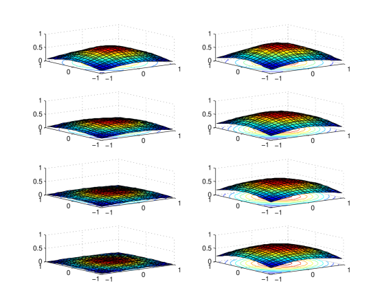
In Fig. 1 some graphs of the solution are displayed. On the left-hand side, one can see the plots of the solution at , , , and , for the non-delay case. On the right-hand side the corresponding plots are depicted, but for the delayed equation, when the propagation speed is . The values of the remaining parameters are , , . In both cases the stepsize in time is , and the parameters of the space discretisation are , . From this figure it is clear that as an effect of the delay, the decay of the solution in the case of the delayed equation is much slower.
4 Conclusions
We have described and analysed a new numerical algorithm for computing approximate solutions of the two-dimensional neural field equations with delay. The stability, convergence and complexity of this algorithm have been analysed and a set of numerical examples has been presented. The numerical experiments are in agreement with the theoretical results and confirm that this algorithm can be successfully used for the solution of problems in Neuroscience and Robotics. The main advantages of the described algorithm are its stability and accuracy, which is illustrated by the presented examples. Moreover, due to the use of a rank reduction technique, it is efficient when dealing with the two-dimensional case.
5 Acknowledgements
This research was supported by a Marie Curie Intra European Fellowship within the 7th European Community Framework Programme (PIEF-GA-2013-629496).
References
- [1] S.L. Amari, Dynamics of pattern formation in lateral-inhibition type neural fields, Biol. Cybernet. 27 (2) (1977) 77–87.
- [2] I. Bojak, D.T.J. Lily, Axonal Velocity Distributions in Neural Field Equations, PLoS Comput Biol 6(1), (2010), e1000653.
- [3] H. Brunner, On the numerical solution of nonlinear Volterra-Fredholm integral equations by collocation methods, SIAM J. Numer. Anal. 27 (1990) 987-1000.
- [4] A. Cardone, E. Messina, and E.Russo, A fast iterative method for discretized Volterra-Fredholm integral equations, J. Comput. Applied Math. 189 (2006) 568-579.
- [5] S. Coombes, Large-scale neural dynamics: Simple and complex, NeuroImage 52, (2010), 731–739.
- [6] S. Coombes, N.A. Venkov, L. Shiau, I. Bojak, D.T.J. Liley, C.R. Laing, Modeling electrocortical activity through improved local approximations of integral neural field equations, Phys. Rev. E 76, (2007), 051901.
- [7] W. Erlhagen, E. Bicho, The dynamic neural field approach to cognitive robotics, J. Neural Eng. 3, (2006), R36-R54.
- [8] G. Faye and O. Faugeras, Some theoretical and numerical results for delayed neural field equations, Physica D 239 (2010) 561–578.
- [9] Han Guoqiang, Asymtotic error expansion for a nonlinear Volterra-Fredholm integral equation, J. Comput. Applied Math. 59 (1995) 49-59.
- [10] A. Hutt and N. Rougier, Activity spread and breathers induced by finite transmission speeds in two-dimensional neuronal fields, Physical Review,E 82 (2010) 055701.
- [11] A. Hutt and N. Rougier, Numerical Simulations of One- and Two-dimensional Neural Fields Involving Space-Dependent Delays, in S. Coombes et al., Eds., Neural Fields Theory and Applications, Springer, 2014.
- [12] Z. Jackiewicz, M. Rahman, B.D. Welfert, Numerical Solution of a Fredholm integro-differential equation modelling neural networks, Applied Numerical Mathematics, 56 (2006) 423-432.
- [13] Z. Jackiewicz, M. Rahman, B.D. Welfert, Numerical Solution of a Fredholm integro-differential equation modelling -neural networks, Appl. Math. Comput., 195 (2008) 523-536.
- [14] J.-P. Kauthen, Continuous time collocation methods for Volterra-Fredholm integral equations, Num. Math. 56 (1989) 409–424.
- [15] R. Potthast and P. beim Graben, Existence and properties of solutions for neural field equations, Math. Meth. Appl. Sci., 33 (2010) 935-949.
- [16] H.R. Wilson and J.D. Cowan, Excitatory and inhibitory interactions in localized populations of model neurons, Bipophys. J., 12 (1972) 1-24.
- [17] Weng-Jing Xie, Fu-Rong Lin, A fast numerical solution method for two dimensional Fredholm integral equations of the second kind, Applied Numerical Mathematics, 59 (2009) 1709-1719.