Multi-Index Stochastic Collocation for random PDEs

Abstract

In this work we introduce the Multi-Index Stochastic Collocation method (MISC) for computing statistics of the solution of a PDE with random data. MISC is a combination technique based on mixed differences of spatial approximations and quadratures over the space of random data. We propose an optimization procedure to select the most effective mixed differences to include in the MISC estimator: such optimization is a crucial step and allows us to build a method that, provided with sufficient solution regularity, is potentially more effective than other multi-level collocation methods already available in literature. We then provide a complexity analysis that assumes decay rates of product type for such mixed differences, showing that in the optimal case the convergence rate of MISC is only dictated by the convergence of the deterministic solver applied to a one dimensional problem. We show the effectiveness of MISC with some computational tests, comparing it with other related methods available in the literature, such as the Multi-Index and Multilevel Monte Carlo, Multilevel Stochastic Collocation, Quasi Optimal Stochastic Collocation and Sparse Composite Collocation methods.

1 Introduction

Uncertainty Quantification (UQ) is an interdisciplinary, fast-growing research area that focuses on devising mathematical techniques to tackle problems in engineering and natural sciences in which only a probabilistic description of the parameters of the governing equations is available, due to measurement errors, intrinsic non-measurability/non-predictability, or incomplete knowledge of the system of interest. In this context, “parameters” is a term used in broad sense to refer to constitutive laws, forcing terms, domain shapes, boundary and initial conditions, etc.

UQ methods can be divided into deterministic and randomized methods. While randomized techniques, which include the Monte Carlo sampling method, are essentially based on random sampling and ensemble averaging, deterministic methods proceed by building a surrogate of the system’s response function over the parameter space, which is then processed to obtain the desired information. Typical goals include computing statistical moments (expected value, variance, higher moments, correlations) of some quantity of interest of the system at hand, typically functionals of the state variables (forward problem), or updating the statistical description of the random parameters given some observations of the system at hand (inverse problem). In any case, multiple resolutions of the governing equations are needed to explore the dependence of the state variables on the random parameters. The computational method used should therefore be carefully designed to minimize the computational effort.

In this work, we focus on the case of PDEs with random data, for which both deterministic and randomized approaches have been extensively explored in recent years. As for the deterministic methods, we mention here the methods based on polynomial expansions computed either by global Galerkin-type projections [1, 2, 3, 4, 5] or collocation strategies based on sparse grids (see e.g. [6, 7, 8, 9]), low-rank techniques [10, 11, 12, 13] and reduced basis methods (see e.g. [14, 15]). All these approaches have been found to be particularly effective when applied to problems with a moderate number of random parameters (low-dimensional probability space) and smooth response functions. Although significant effort has been expended on increasing the efficiency of such deterministic methods with respect to the number of random parameters (see, e.g., [16], the seminal work on infinite dimensional polynomial approximation of elliptic PDEs with random coefficients), Monte Carlo-type approximations remain the primary choice for problems with non-smooth response functions and/or those that depend on a high number of random parameters, despite their slow convergence with respect to sample size.

A very promising methodology that builds on the classical Monte Carlo method and enhances its performance is offered by the so-called Multilevel Monte Carlo (MLMC). It was first proposed in [17] for applications in parametric integration and extended to weak approximation of stochastic differential equations in [18], which also provided a full complexity analysis. Let $\{h_{\ell}\}_{\ell=0}^{L}$ be a (scalar) sequence of spatial/temporal resolution levels that can be used for the numerical discretization of the PDE at hand and $\{F_{\ell}\}_{\ell=0}^{L}$ be the corresponding approximations of the quantity of interest, and suppose that the final goal of the UQ analysis is to compute the expected value of $F$, ${\mathbb{E}\mspace{-2.0mu}\left[F\right]}$. While a classic Monte Carlo approach simply approximates the expected value by using an ensemble average over a sample of independent replicas of the random parameters, the MLMC method relies on the simple observation that, by linearity of expectation,

$${\mathbb{E}\mspace{-2.0mu}\left[F\right]}\approx{\mathbb{E}\mspace{-2.0mu}\left[F_{L}\right]}={\mathbb{E}\mspace{-2.0mu}\left[F_{0}\right]}+\sum_{\ell=1}^{L}{\mathbb{E}\mspace{-2.0mu}\left[F_{\ell}-F_{\ell-1}\right]},$$ (1)

and computes by independent Monte Carlo samplers each expectation in the sum. Indeed, if the discretization of the underlying differential model is converging with respect to the discretization level, $\ell$, the variance of $(F_{\ell}-F_{\ell-1})$ will be smaller and smaller as $\ell$ increases, i.e., when the spatial/temporal resolution increases. Dramatic computational saving can thus be obtained by approximating the quantities ${\mathbb{E}\mspace{-2.0mu}\left[F_{\ell}-F_{\ell-1}\right]}$ with a smaller and smaller sample size, since most of the variability of $F$ will be captured with coarse simulations and only a few resolutions over the finest discretization levels will be performed. The MLMC estimator is therefore given by

$${\mathbb{E}\mspace{-2.0mu}\left[F\right]}\approx\sum_{\ell=0}^{L}\frac{1}{M_{\ell}}\sum_{m=1}^{M_{\ell}}\left(F_{\ell}(\omega_{m,\ell})-F_{\ell-1}(\omega_{m,\ell})\right),\quad\text{with }F_{-1}(\cdot)=0,$$ (2)

where $\omega_{m,\ell}$ are the i.i.d. replicas of the random parameters. The application of MLMC methods to UQ problems involving PDEs with random data has been investigated from the mathematical point of view in a number of recent publications, see e.g. [19, 20, 21, 22, 23]. Recent works [24, 25, 26, 27] have explored the possibility of replacing the Monte Carlo sampler on each level by other quadrature formulas such as sparse grids or quasi-Monte Carlo quadrature, obtaining the so-called Multilevel Stochastic Collocation (MLSC) or Multilevel Quasi-Monte Carlo (MLQCM) methods. See also [28] for a related approach where the Multilevel Monte Carlo method is combined with a control variate technique.

The starting point of this work is instead the so-called Multi-Index Monte Carlo method (MIMC), recently introduced in [29], that differs from the Multilevel Monte Carlo method in that the telescoping idea presented in equations (1)-(2) is applied to discretizations indexed by a multi-index rather than a scalar index, thus allowing each discretization parameter to vary independently of the others. Analogously to what done in [24, 25, 26] in the context of stochastic collocation, here we propose to replace the Monte Carlo quadrature with a sparse grid quadrature at each telescopic level, obtaining in our case the Multi-Index Stochastic Collocation method (MISC). In other words, MISC can be seen as a multi-index version of MLSC, or a stochastic collocation version of MIMC. From a slightly different perspective, MISC is also closely related to the combination technique developed for the solution of (deterministic) PDEs in [30, 7, 31, 32, 33]; in this work, the combination technique is used with respect to both the deterministic and stochastic variables.

One key difference between the present work and [24, 25, 26] is that the number of problem solves to be performed at each discretization level is not determined by balancing the spatial and stochastic components of the error (based, e.g., on convergence error estimates), but rather suitably extending the knapsack-problem approach that we employed in [34, 35, 36] to derive the so-called Quasi-Optimal Sparse Grids method (see also [37]). A somewhat analogous approach was proposed in [38], where the number of solves per discretization level is prescribed a-priori based on a standard sparsification procedure (we will give more details on the comparison between these different methods later on). In this work, we provide a complexity analysis of MISC and illustrate its performance improvements, comparing it to other methods by means of numerical examples.

The remainder of this paper is organized as follows. In Section 2, we introduce the problem to be solved and the approximation schemes that will be used. The Multi-Index Stochastic Collocation method is introduced in Section 3, and our main theorem detailing the complexity of MISC for a particular choice of an index set is presented in Section 4. Finally, Section 5 presents some numerical tests, while Section 6 offers some conclusions and final remarks. The Appendix contains the technical proof of the main theorem. Throughout the rest of this work we use the following notation:

• $\mathbb{N}$ denotes the set of integer numbers including zero;

• $\mathbb{N}_{+}$ denotes the set of positive integer numbers, i.e. excluding zero;

• $\mathbb{R}_{+}$ denotes the set of positive real numbers, $\mathbb{R}_{+}=\{r\in\mathbb{R}:r>0\}$;

• $\bm{1}$ denotes a vector whose components are always equal to one;

• ${{\bm{e}}}^{\kappa}_{\ell}$ denotes the $\ell$-th canonical vector in $\mathbb{R}^{\kappa}$, i.e., $({{\bm{e}}}^{\kappa}_{\ell})_{i}=1$ if $\ell=i$ and zero otherwise; however, for the sake of clarity, we often omit the superscript $\kappa$ when obvious from the context. For instance, if ${{\bm{v}}}\in\mathbb{R}^{N}$, we will write ${{\bm{v}}}-{{\bm{e}}}_{1}$ instead of ${{\bm{v}}}-{{\bm{e}}}_{1}^{N}$;

• given ${{\bm{v}}}\in\mathbb{R}^{N}$, $|{{\bm{v}}}|=\sum_{n=1}^{N}v_{n}$, $\max({{\bm{v}}})=\max_{n=1,\ldots N}v_{n}$ and $\min({{\bm{v}}})=\min_{n=1,\ldots N}v_{n}$;

• given ${{\bm{v}}}\in\mathbb{R}^{N}$ and $f:\mathbb{R}\to\mathbb{R}$, $f({{\bm{v}}})$ denotes the vector obtained by applying $f$ to each component of ${{\bm{v}}}$, $f({{\bm{v}}})=[f(v_{1}),f(v_{2}),\cdots,f(v_{N})]\in\mathbb{R}^{N}$;

• given ${{\bm{v}}},{{\bm{w}}}\in\mathbb{R}^{N}$, the inequality ${{\bm{v}}}>{{\bm{w}}}$ holds true if and only if $v_{n}>w_{n}$ $\forall n=1,\ldots,N$.

• given ${{\bm{v}}}\in\mathbb{R}^{D}$ and ${{\bm{w}}}\in\mathbb{R}^{N}$, $[{{\bm{v}}},{{\bm{w}}}]=(v_{1},\ldots,v_{D},w_{1},\ldots,w_{N})\in\mathbb{R}^{D+N}$.

2 Problem setting

Let $\mathscr{B}\subset\mathbb{R}^{d}$, $d=1,2,3$, be an open hyper-rectangular domain (referred to hereafter as the “physical domain”) and let ${{\bm{y}}}=(y_{1},y_{2},\ldots,y_{N})$ be a $N$-dimensional random vector whose components are mutually independent and uniformly distributed random variables with support $\Gamma_{n}\subset\mathbb{R}$ and probability density function $\rho_{n}(y_{n})=\frac{1}{|\Gamma_{n}|}$. Denoting $\Gamma=\Gamma_{1}\times\Gamma_{2}\ldots\times\Gamma_{N}$ (referred to hereafter as the “stochastic domain” or “parameter space”) and by $\sigma_{B}(\Gamma)$ the Borel $\sigma$-algebra over $\Gamma$, $\rho({{\bm{y}}})d{{\bm{y}}}=\prod_{n=1}^{N}\rho_{n}(y_{n})dy_{n}$ is therefore a probability measure on $\Gamma$, due to the independence of $y_{n}$, and $(\Gamma,\sigma_{B}(\Gamma),\rho({{\bm{y}}})d{{\bm{y}}})$ is a complete probability space. Consider the following generic PDE, together with the assumption stated next:

Problem 1.

Find $u:\mathscr{B}\times\Gamma\rightarrow\mathbb{R}$ such that for $\rho$-almost every ${{\bm{y}}}\in\Gamma$

$$\begin{cases}\mathcal{L}(u;{{\bm{x}}},{{\bm{y}}})=\mathscr{F}({{\bm{x}}})&{{\bm{x}}}\in\mathscr{B},\\ u({{\bm{x}}},{{\bm{y}}})=0&{{\bm{x}}}\in\partial\mathscr{B}.\end{cases}$$

Assumption 1 (Well posedness).

Problem 1 is well posed in some Hilbert space $V$ for $\rho$-almost every ${{\bm{y}}}\in\Gamma$.

The solution of Problem 1 can be seen as an $N$-variate Hilbert-space valued function $u({{\bm{y}}}):\Gamma\rightarrow V$. The random variables, $y_{n}$, can represent scalar values whose exact value is unknown, or they can stem from a spectral decomposition of a random field, like a Karhunen-Loève or Fourier expansion, possibly truncated after a finite number of terms, see, e.g., [6, 36]. It is also useful to introduce the Bochner space $L^{2}_{\rho}(\Gamma;V)=\left\{u:\Gamma\rightarrow V\mbox{ strongly measurable s.t. }\int_{\Gamma}\|u({{\bm{y}}})\|_{V}^{2}\rho({{\bm{y}}})d{{\bm{y}}}<\infty\right\}.$ Finally, given some functional of the solution $u$, $\Theta:V\rightarrow\mathbb{R}$, we denote by $F:\Gamma\rightarrow\mathbb{R}$ the $N$-variate real-valued function assigning to each realization ${{\bm{y}}}\in\Gamma$ the corresponding value of $\Theta[u]$ (quantity of interest), i.e., $F({{\bm{y}}})=\Theta[u(\cdot,{{\bm{y}}})]$, and we aim at estimating its expected value,

$${\mathbb{E}\mspace{-2.0mu}\left[F\right]}=\int_{\Gamma}F({{\bm{y}}})\rho({{\bm{y}}})d{{\bm{y}}}.$$

Example 1.

As a motivating example, consider the following elliptic problem: find $u:\mathscr{B}\times\Gamma\rightarrow\mathbb{R}$ such that for $\rho$-almost every ${{\bm{y}}}\in\Gamma$

$$\begin{cases}-\textnormal{div}(a({{\bm{x}}},{{\bm{y}}})\nabla u({{\bm{x}}},{{\bm{y}}}))=\mathscr{F}({{\bm{x}}})&{{\bm{x}}}\in\mathscr{B},\\ u({{\bm{x}}},{{\bm{y}}})=h({{\bm{x}}})&{{\bm{x}}}\in\partial\mathscr{B},\end{cases}$$ (3)

holds, where div and $\nabla$ denote differentiation with respect to the physical variables, ${{\bm{x}}}$, only, and the function $a:\mathscr{B}\times\Gamma\rightarrow\mathbb{R}$ is bounded away from $0$ and $\infty$, i.e., there exist two constants, $a_{min},a_{max}$, such that

$$0<a_{min}\leq a({{\bm{x}}},{{\bm{y}}})\leq a_{max}<\infty,\quad\forall{{\bm{x}}}\in\mathscr{B}\mbox{ and for }\rho\mbox{-almost every }{{\bm{y}}}\in\Gamma.$$ (4)

This boundedness condition guarantees that Assumption 1 is satisfied, i.e. the equation is well posed for $\rho$-almost every ${{\bm{y}}}\in\Gamma$, thanks to a straightforward application of the Lax-Milgram lemma; moreover, the equation is well posed in $L^{2}_{\rho}(\Gamma;V)$, where $V$ is the classical Sobolev space $H^{1}_{0}(\mathscr{B})$, see, e.g., [6]. This is the example we will focus on in Section 5, where we will test numerically the performance of the Multi-Index Stochastic Collocation method that we will detail in Section 3.

Remark 1.

The method that we present in the following sections can be also applied to more general problems than Problem 1  in which the forcing terms, boundary conditions and possibly domain shape are also modeled as uncertain; the extension to time-dependent problems with uncertain initial conditions is also straightforward. Other probability measures can also be considered; the very relevant case in which the random variables, $y_{n}$, are normally distributed is an example.

Remark 2.

As will be clearer in a moment, the methodology we propose uses tensorized solvers for deterministic PDEs. Although for ease of exposition we have assumed that the spatial domain, $\mathscr{B}$, is a hyper-rectangle, it is important to remark that the methodology proposed in this work can also be applied to non hyper-rectangular domains: this can be achieved by introducing a mapping from a reference hyper-rectangle to the generic domain of interest (with techniques such as those proposed in the context of Isogeometric Analysis [39] or Transfinite Interpolation [40]) or by a Domain Decomposition approach [41] if the domain can be obtained as a union of hyper-rectangles.

2.1 Approximation along the deterministic and stochastic dimensions

In practice, we can only access the value of $F$ via a numerical solver yielding a numerical approximation of the solution $u$ of Problem 1, which depends on a set of $D$ discretization parameters, such as the mesh-size, the time-step, the tolerances of the numerical solvers, and others, which we denote by $h_{i},i=1,\ldots,D$; we remark that in general $D$, the number of parameters, might be different from $d$, the number of spatial dimensions. For each of those parameters, we introduce a sequence of discretization levels, $h_{i,\alpha},\alpha=1,2,\ldots$, and for each multi-index ${{{\bm{\alpha}}}}\in\mathbb{N}^{D}_{+}$, we denote by $u^{{{\bm{\alpha}}}}({{\bm{x}}},{{\bm{y}}})$ the approximation of $u$ obtained from setting $h_{i}=h_{i,\alpha_{i}}$, with the implicit assumption that $u^{{{\bm{\alpha}}}}({{\bm{x}}},{{\bm{y}}})\to u({{\bm{x}}},{{\bm{y}}})$ as $\min_{1\leq i\leq D}\alpha_{i}\to\infty$ for $\rho$-almost every ${{\bm{y}}}\in\Gamma$; similarly, we also write $F^{{{\bm{\alpha}}}}({{\bm{y}}})=\Theta[u^{{{\bm{\alpha}}}}(\cdot,{{\bm{y}}})]$. For instance, we could solve the problem stated in Example 1 by a finite differences scheme with grid-sizes $h_{i,\alpha_{i}}=h_{0}2^{-\alpha_{i}}$ in direction $i=1,\ldots,D$, for some $h_{0}>0$.

The discretization of $F^{{{\bm{\alpha}}}}$ over the random parameter space $\Gamma$ will consist of a suitable linear combination of tensor interpolants over $\Gamma$ based on Lagrangian polynomials. Observe that this approach is sound only if $F^{{{\bm{\alpha}}}}$ is at least a continuous function over $\Gamma$ (the smoother $F^{{{\bm{\alpha}}}}$ is, the more effective the Lagrangian approximation will be); for instance, for the problem stated in Example 1, it can be shown under moderate assumptions on $a({{\bm{x}}},{{\bm{y}}})$ that $F$ and $F^{{{\bm{\alpha}}}}$ are ${{\bm{y}}}$-analytic, see, e.g., [35, 16]; we will return to this point in Section 5.

To derive a generic tensor Lagrangian interpolation of $F^{{{\bm{\alpha}}}}$, we first introduce the set $\mathcal{C}^{0}(\Gamma_{n})$ of real-valued continuous functions over $\Gamma_{n}$, and the subspace of polynomials of degree at most $q$ over $\Gamma_{n}$, $\mathbb{P}^{q}(\Gamma_{n})\subset\mathcal{C}^{0}(\Gamma_{n})$. Next, we consider a sequence of univariate Lagrangian interpolant operators in each dimension $Y_{n}$, i.e., $\{\mathscr{U}_{n}^{m(\beta_{n})}\}_{\beta_{n}\in\mathbb{N}_{+}}$, where we refer to the value $\beta_{n}$ as the “interpolation level”. Each interpolant is built over a set of $m(\beta_{n})$ collocation points, $\mathscr{H}_{n}^{m(\beta_{n})}=\{y_{n}^{1},y_{n}^{2}\ldots y_{n}^{m(\beta_{n})}\}\subset\Gamma_{n}$, where $m$ is a strictly increasing function, with $m(0)=0$ and $m(1)=1$, that we call the “level-to-nodes function”; thus, the interpolant yields a polynomial approximation,

$$\mathscr{U}^{m(\beta_{n})}_{n}:\mathcal{C}^{0}(\Gamma_{n})\rightarrow\mathbb{P}^{m(\beta_{n})-1}(\Gamma_{n}),\qquad\mathscr{U}^{m(\beta_{n})}_{n}[f](y_{n})=\sum_{j=1}^{m(\beta_{n})}\left(f(y_{n}^{j})\prod_{k=1,k\neq j}^{m(\beta_{n})}\frac{y_{n}-y_{n}^{k}}{y^{j}_{n}-y_{n}^{k}}\right),$$

with the convention that $\mathscr{U}^{0}_{n}[f]=0\,\,\forall f\in\mathcal{C}^{0}(\Gamma_{n})$.

The $N$-variate Lagrangian interpolant can then be built by a tensorization of univariate interpolants: denote by $\mathcal{C}^{0}(\Gamma)$ the space of real-valued $N$-variate continuous functions over $\Gamma$ and by $\mathbb{P}^{{\bm{q}}}(\Gamma)=\bigotimes_{n=1}^{N}\mathbb{P}^{q_{n}}(\Gamma_{n})$ the subspace of polynomials of degree at most $q_{n}$ over $\Gamma_{n}$, with ${{\bm{q}}}=(q_{1},\ldots,q_{N})\in\mathbb{N}^{N}$, and consider a multi-index ${{{\bm{\beta}}}}\in\mathbb{N}_{+}^{N}$ assigning the interpolation level in each direction, $y_{n}$; the multivariate interpolant can then be written as

$$\mathscr{U}^{m({{{\bm{\beta}}}})}:\mathcal{C}^{0}(\Gamma)\rightarrow\mathbb{P}^{m({{{\bm{\beta}}}})-\bm{1}}(\Gamma),\qquad\mathscr{U}^{m({{{\bm{\beta}}}})}[F^{{{\bm{\alpha}}}}]({{\bm{y}}}) =\left(\mathscr{U}^{m(\beta_{1})}_{1}\otimes\cdots\otimes\mathscr{U}^{m(\beta_{N})}_{N}\right)[F^{{{\bm{\alpha}}}}]({{\bm{y}}}).$$

The set of collocation points needed to build the tensor interpolant $\mathscr{U}^{m({{{\bm{\beta}}}})}[u]({{\bm{y}}})$ is the tensor grid $\mathscr{T}^{m({{{\bm{\beta}}}})}=\times_{n=1}^{N}\mathscr{H}_{n}^{m(\beta_{n})}$ with cardinality $\#\mathscr{T}^{m({{{\bm{\beta}}}})}=\prod_{n=1}^{N}m(\beta_{n})$. Observe that the Lagrangian interpolant immediately induces an $N$-variate quadrature formula, $\mathscr{Q}^{m({{{\bm{\beta}}}})}:\mathcal{C}^{0}(\Gamma)\rightarrow\mathbb{R}$,

$$\mathscr{Q}^{m({{{\bm{\beta}}}})}[F^{{{\bm{\alpha}}}}]={\mathbb{E}\mspace{-2.0mu}\left[{\mathscr{U}}^{m({{{\bm{\beta}}}})}[F^{{{\bm{\alpha}}}}]({{\bm{y}}})\right]}=\sum_{j=1}^{\#\mathscr{T}^{m({{{\bm{\beta}}}})}}F^{{{\bm{\alpha}}}}(\widehat{{{\bm{y}}}}_{j})\varpi_{j},$$

where $\widehat{{{\bm{y}}}}_{j}\in\mathscr{T}^{m({{{\bm{\beta}}}})}$ and the quadrature weights $\varpi_{j}$ are the expected values of the Lagrangian polynomials centered in $\widehat{{{\bm{y}}}}_{j}$, which can be computed exactly for most of the common interpolation knots and probability measures of the random variables.

It is recommended that the collocation points $\mathscr{H}_{n}^{m(\beta_{n})}$ to be used in each direction are chosen according to the underlying probability measure, $\rho(y_{n})dy_{n}$, to ensure good approximation properties of the interpolant and quadrature operators, $\mathscr{U}^{m({{{\bm{\beta}}}})}$ and $\mathscr{Q}^{m({{{\bm{\beta}}}})}$. Common choices are Gaussian quadrature points like Gauss-Legendre for uniform measures or Gauss-Hermite for Gaussian measures, cf. e.g., [42], which are however not nested, i.e., $\mathscr{H}_{n}^{m(\beta_{n})}\not\subset\mathscr{H}_{n}^{m(\beta_{n}+1)}$. This means that they are not optimal for successive refinements of the interpolation/quadrature, and we will not consider them in this work. Instead, we will work with nested collocation points, and specifically with Clenshaw-Curtis points [34, 43], that are a classical choice for the uniform measure that we are considering here; other choices of nested points are available for uniform random variables, e.g., the Leja points [34, 44], whose performance is somehow equivalent to that of Clenshaw-Curtis for quadrature purposes, see [45, 46]. Clenshaw-Curtis points are defined as

$$y_{n}^{j}=\cos\left(\frac{(j-1)\pi}{m(i_{n})-1}\right),\quad 1\leq j\leq m(i_{n}),$$ (5)

together with the following level-to-nodes relation, $m(i_{n})$, that ensures their nestedness:

$$m(0)=0,\,\,m(1)=1,\,\,m(i_{n})=2^{i_{n}-1}+1.$$ (6)

We conclude this section by introducing the following operator norm, which acts as a “Lebesgue constant” from $\mathcal{C}^{0}(\Gamma)$ to $L^{2}_{\rho}(\Gamma)$:

$$\mathbb{M}^{m({{{\bm{\beta}}}})}=\prod_{n=1}^{N}\mathbb{M}_{n}^{m(\beta_{n})},\quad\mbox{with }\quad\mathbb{M}_{n}^{m(\beta_{n})}=\sup_{\|f\|_{L^{\infty}(\Gamma_{n})}=1}\|\mathscr{U}^{m(\beta_{n})}_{n}f\|_{L^{2}_{\rho}(\Gamma_{n})}.$$ (7)

In particular, for the Clenshaw-Curtis points, it is possible to bound $\mathbb{M}_{n}^{m(\beta_{n})}$ as:

$$\mathbb{M}^{m({{{\bm{\beta}}}})}\leq\mathbb{M}_{est}^{m({{{\bm{\beta}}}})}=\prod_{n=1}^{N}\mathbb{M}_{n,est}^{m(\beta_{n})},\quad\quad\mathbb{M}_{n,est}^{q}=\begin{cases}1&\mbox{ for }q=1\\[5.69054pt] \displaystyle\frac{2}{\pi}\log(q-1)+1&\mbox{ for }q\geq 2.\end{cases}$$ (8)

See [34] and references therein.

Remark 3.

Nested collocation points have been studied also for other probability measures than uniform probability measures. In the very relevant case of a normal distribution, one possible choice is the Genz-Keister points [47, 36]; we mention also the recent work [46] on generalized Leja points that can be used for arbitrary measures on unbounded domains.

3 Multi-Index Stochastic Collocation

It is easy to see that an accurate approximation of ${\mathbb{E}\mspace{-2.0mu}\left[F\right]}$ by a direct tensor technique as the one just introduced, ${\mathbb{E}\mspace{-2.0mu}\left[F\right]}\approx\mathscr{Q}^{m({{{\bm{\beta}}}})}[F^{{{\bm{\alpha}}}}]$, might require a prohibitively large computational effort even for moderate values of $D$ and $N$ (what is referred to as the “curse of dimensionality”). In this work, following the setting that was presented in [34, 29], we propose the Multi-Index Stochastic Collocation as an alternative. It can be seen as a generalization of the telescoping sum presented in the introduction, see equations (1) and (2). Denoting $\mathscr{Q}^{m({{{\bm{\beta}}}})}[F^{{{\bm{\alpha}}}}]=F_{{{{\bm{\alpha}}}},{{{\bm{\beta}}}}}$, the building blocks of such a telescoping sum are the first-order difference operators for the deterministic and stochastic discretization parameters, denoted respectively by $\Delta_{i}^{\textnormal{det}}$ with $1\leq i\leq D$ and $\Delta_{j}^{\textnormal{stoc}}$ with $1\leq j\leq N$:

$$\Delta_{i}^{\textnormal{det}}[F_{{{{\bm{\alpha}}}},{{{\bm{\beta}}}}}]=\begin{cases}F_{{{{\bm{\alpha}}}},{{{\bm{\beta}}}}}-F_{{{{\bm{\alpha}}}}-{{\bm{e}}}_{i},{{{\bm{\beta}}}}},&\text{if }\alpha_{i}>1,\\ F_{{{{\bm{\alpha}}}},{{{\bm{\beta}}}}}&\text{if }\alpha_{i}=1,\end{cases}$$ (9)

$$\Delta_{j}^{\textnormal{stoc}}[F_{{{{\bm{\alpha}}}},{{{\bm{\beta}}}}}]=\begin{cases}F_{{{{\bm{\alpha}}}},{{{\bm{\beta}}}}}-F_{{{{\bm{\alpha}}}},{{{\bm{\beta}}}}-{{\bm{e}}}_{j}},&\text{if }\beta_{j}>1,\\ F_{{{{\bm{\alpha}}}},{{{\bm{\beta}}}}}&\text{if }\beta_{j}=1.\end{cases}$$ (10)

We then define the first-order tensor difference operators,

$${{\bm{\Delta}}}^{\textnormal{det}}[F_{{{{\bm{\alpha}}}},{{{\bm{\beta}}}}}]=\bigotimes_{i=1}^{D}\Delta_{i}^{\textnormal{det}}[F_{{{{\bm{\alpha}}}},{{{\bm{\beta}}}}}]=\Delta_{1}^{\textnormal{det}}\left[\,\Delta_{2}^{\textnormal{det}}\left[\,\cdots\Delta_{D}^{\textnormal{det}}\left[F_{{{{\bm{\alpha}}}},{{{\bm{\beta}}}}}\right]\,\right]\,\right]=\sum_{{{\bm{j}}}\in\{0,1\}^{D}}(-1)^{|{{\bm{j}}}|}F_{{{{\bm{\alpha}}}}-{{\bm{j}}},{{{\bm{\beta}}}}},$$ (11)

$${{\bm{\Delta}}}^{\textnormal{stoc}}[F_{{{{\bm{\alpha}}}},{{{\bm{\beta}}}}}]=\bigotimes_{j=1}^{N}\Delta_{j}^{\textnormal{stoc}}[F_{{{{\bm{\alpha}}}},{{{\bm{\beta}}}}}]=\sum_{{{\bm{j}}}\in\{0,1\}^{N}}(-1)^{|{{\bm{j}}}|}F_{{{{\bm{\alpha}}}},{{{\bm{\beta}}}}-{{\bm{j}}}}\,.$$ (12)

with the convention that $F_{{{\bm{v}}},{{\bm{w}}}}=0$ whenever a component of ${{\bm{v}}}$ or ${{\bm{w}}}$ is zero. Observe that computing ${{\bm{\Delta}}}^{\textnormal{det}}[F_{{{{\bm{\alpha}}}},{{{\bm{\beta}}}}}]$ actually requires up to $2^{D}$ solver calls, and analogously applying ${{\bm{\Delta}}}^{\textnormal{stoc}}[F_{{{{\bm{\alpha}}}},{{{\bm{\beta}}}}}]$ requires interpolating $F^{{{\bm{\alpha}}}}$ on up to $2^{N}$ tensor grids; for instance, if $D=N=2$ and ${{{\bm{\alpha}}}},{{{\bm{\beta}}}}>\bm{1}$, we have

$${{\bm{\Delta}}}^{\textnormal{det}}[F_{{{{\bm{\alpha}}}},{{{\bm{\beta}}}}}]=\Delta^{\textnormal{det}}_{2}\left[\,\Delta^{\textnormal{det}}_{1}\left[\,F_{{{{\bm{\alpha}}}},{{{\bm{\beta}}}}}\,\right]\,\right]=\Delta^{\textnormal{det}}_{2}[F_{{{{\bm{\alpha}}}},{{{\bm{\beta}}}}}-F_{{{{\bm{\alpha}}}}-{{\bm{e}}}_{1},{{{\bm{\beta}}}}}]=F_{{{{\bm{\alpha}}}},{{{\bm{\beta}}}}}-F_{{{{\bm{\alpha}}}}-{{\bm{e}}}_{1},{{{\bm{\beta}}}}}-F_{{{{\bm{\alpha}}}}-{{\bm{e}}}_{2},{{{\bm{\beta}}}}}+F_{{{{\bm{\alpha}}}}-\bm{1},{{{\bm{\beta}}}}},$$

$${{\bm{\Delta}}}^{\textnormal{stoc}}[F_{{{{\bm{\alpha}}}},{{{\bm{\beta}}}}}]=F_{{{{\bm{\alpha}}}},{{{\bm{\beta}}}}}-F_{{{{\bm{\alpha}}}},{{{\bm{\beta}}}}-{{\bm{e}}}_{1}}-F_{{{{\bm{\alpha}}}},{{{\bm{\beta}}}}-{{\bm{e}}}_{2}}+F_{{{{\bm{\alpha}}}},{{{\bm{\beta}}}}-\bm{1}}.$$

Finally, letting ${{\bm{\Delta}}}[F_{{{{\bm{\alpha}}}},{{{\bm{\beta}}}}}]={{\bm{\Delta}}}^{\textnormal{stoc}}[{{\bm{\Delta}}}^{\textnormal{det}}[F_{{{{\bm{\alpha}}}},{{{\bm{\beta}}}}}]]$, we define the Multi-Index Stochastic Collocation (MISC) estimator of ${\mathbb{E}\mspace{-2.0mu}\left[F\right]}$ as

$$\mathscr{M}_{\mathcal{I}}[F]=\sum_{[{{{\bm{\alpha}}}},{{{\bm{\beta}}}}]\in\mathcal{I}}{{\bm{\Delta}}}[F_{{{{\bm{\alpha}}}},{{{\bm{\beta}}}}}]=\sum_{[{{{\bm{\alpha}}}},{{{\bm{\beta}}}}]\in\mathcal{I}}c_{{{{\bm{\alpha}}}},{{{\bm{\beta}}}}}F_{{{{\bm{\alpha}}}},{{{\bm{\beta}}}}},$$ (13)

where $\mathcal{I}\subset\mathbb{N}_{+}^{D+N}$ and $c_{{{{\bm{\alpha}}}},{{{\bm{\beta}}}}}\in\mathbb{Z}$. Observe that many of the coefficients in (13), $c_{{{{\bm{\alpha}}}},{{{\bm{\beta}}}}}$, may be zero: in particular, $c_{{{{\bm{\alpha}}}},{{{\bm{\beta}}}}}$ is zero whenever $[{{{\bm{\alpha}}}},{{{\bm{\beta}}}}]+{{\bm{j}}}\in\mathcal{I}$ $\forall{{\bm{j}}}\in\{0,1\}^{N+D}$. Similarly to the analogous sparse grid construction [34, 48, 7], we shall require that the multi-index set $\mathcal{I}$ be downward closed, i.e.,

$$\forall\,[{{{\bm{\alpha}}}},{{{\bm{\beta}}}}]\in\mathcal{I},\quad\begin{cases}{{{\bm{\alpha}}}}-{{\bm{e}}}_{i}\in\mathcal{I}\mbox{ for }1\leq i\leq D\mbox{ and }\alpha_{i}>1,\\ {{{\bm{\beta}}}}-{{\bm{e}}}_{j}\in\mathcal{I}\mbox{ for }1\leq j\leq N\mbox{ and }\beta_{j}>1.\end{cases}$$

Remark 4.

In theory, a MISC approach could also be developed to approximate the entire solution $u({{\bm{x}}},{{\bm{y}}})$ and not just the expectation of functionals, considering differences between consecutive interpolant operators, $\mathscr{U}^{m({{{\bm{\beta}}}})}$, on the stochastic domain rather than differences of the quadrature operators, $\mathscr{Q}^{m({{{\bm{\beta}}}})}$, as a building block for the ${{\bm{\Delta}}}^{\textnormal{stoc}}$ operators, as well as considering the discretized solution $u^{{{\bm{\alpha}}}}$ rather than just the quantity of interest, $F^{{{\bm{\alpha}}}}$, in the construction of the ${{\bm{\Delta}}}^{\textnormal{det}}$ operators.

3.1 A knapsack-like construction of the set $\mathcal{I}$

The efficiency of the MISC method in equation (13) will heavily depend on the specific choice of the index set, $\mathcal{I}$; in the following, we will first propose a general strategy to derive quasi-optimal sets and then prove in Section 4 a convergence result for such sets under some reasonable assumptions.

To derive an efficient set, $\mathcal{I}$, we recast the problem of its construction as an optimization problem, in the same spirit of [29, 34, 35, 7, 37]. We begin by introducing the concepts of “work contribution”, $\Delta W_{{{{\bm{\alpha}}}},{{{\bm{\beta}}}}}$, and “error contribution”, $\Delta E_{{{{\bm{\alpha}}}},{{{\bm{\beta}}}}}$, for each hierarchical surplus operator, ${{\bm{\Delta}}}[F_{{{{\bm{\alpha}}}},{{{\bm{\beta}}}}}]$. The work contribution measures the computational cost (measured, e.g., as a function of the total number of degrees of freedom, or in terms of computational time) required to add ${{\bm{\Delta}}}[F_{{{{\bm{\alpha}}}},{{{\bm{\beta}}}}}]$ to $\mathscr{M}_{\mathcal{I}}[F]$, i.e., to solve the associated deterministic problems and to compute the corresponding interpolants over the parameter space, cf. equations (11) and (12); the error contribution measures instead how much the error $|{\mathbb{E}\mspace{-2.0mu}\left[F\right]}-\mathscr{M}_{\mathcal{I}}[F]|$ would decrease once the operator ${{\bm{\Delta}}}[F_{{{{\bm{\alpha}}}},{{{\bm{\beta}}}}}]$ has been added to $\mathscr{M}_{\mathcal{I}}[F]$. In formulas, we define

$$\Delta W_{{{{\bm{\alpha}}}},{{{\bm{\beta}}}}}={\mathrm{Work}\mspace{-2.0mu}\left[\mathscr{M}_{\mathcal{I}\cup\{[{{{\bm{\alpha}}}},{{{\bm{\beta}}}}]\}}[F]\right]}-{\mathrm{Work}\mspace{-2.0mu}\left[\mathscr{M}_{\mathcal{I}}[F]\right]}={\mathrm{Work}\mspace{-2.0mu}\left[{{\bm{\Delta}}}[F_{{{{\bm{\alpha}}}},{{{\bm{\beta}}}}}]\right]},$$

so that

$${\mathrm{Work}\mspace{-2.0mu}\left[\mathscr{M}_{\mathcal{I}}[F]\right]}=\sum_{[{{{\bm{\alpha}}}},{{{\bm{\beta}}}}]\in\mathcal{I}}\Delta W_{{{{\bm{\alpha}}}},{{{\bm{\beta}}}}},$$ (14)

Observe that this work definition is sharp only if we think of building the MISC estimator with an incremental approach, i.e., we assume that adding the multi-index $({{{\bm{\alpha}}}},{{{\bm{\beta}}}})$ to the index set $\mathcal{I}$ would not reduce the work that has to be done to evaluate the MISC estimator on the index set. This implies that one cannot take advantage of the fact that some of the coefficients in (13), $c_{{{{\bm{\alpha}}}},{{{\bm{\beta}}}}}$, that are non-zero when considering the set $\mathcal{I}$ could become zero if the MISC estimator is instead built considering the set $\mathcal{I}\cup\{[{{{\bm{\alpha}}}},{{{\bm{\beta}}}}]\}$, hence it would be possible not to compute the corresponding approximations $F_{{{{\bm{\alpha}}}},{{{\bm{\beta}}}}}$. This approach is discussed in Section 5.3.

Similarly, we define

$$\Delta E_{{{{\bm{\alpha}}}},{{{\bm{\beta}}}}}=\Big{|}{\mathscr{M}_{\mathcal{I\cup\{[{{{\bm{\alpha}}}},{{{\bm{\beta}}}}]\}}}[F]}-{\mathscr{M}_{\mathcal{I}}[F]}\Big{|}=\left|{{{\bm{\Delta}}}[F_{{{{\bm{\alpha}}}},{{{\bm{\beta}}}}}]}\right|.$$

Thus, by construction, the error of the MISC estimator (13) can be bounded as the sum of the error contributions not included in the estimator $\mathscr{M}_{\mathcal{I}}[F]$,

$${\mathrm{Error}\mspace{-2.0mu}\left[\mathscr{M}_{\mathcal{I}}[F]\right]}=|{\mathbb{E}\mspace{-2.0mu}\left[F\right]}-\mathscr{M}_{\mathcal{I}}[F]| =\left|{\sum_{[{{{\bm{\alpha}}}},{{{\bm{\beta}}}}]\notin\mathcal{I}}{{\bm{\Delta}}}[F_{{{{\bm{\alpha}}}},{{{\bm{\beta}}}}}]}\right|$$

$$\leq\sum_{[{{{\bm{\alpha}}}},{{{\bm{\beta}}}}]\notin\mathcal{I}}\left|{{{\bm{\Delta}}}[F_{{{{\bm{\alpha}}}},{{{\bm{\beta}}}}}]}\right|=\sum_{[{{{\bm{\alpha}}}},{{{\bm{\beta}}}}]\notin\mathcal{I}}\Delta E_{{{{\bm{\alpha}}}},{{{\bm{\beta}}}}}.$$ (15)

Consequently, a quasi-optimal set $\mathcal{I}$ can be computed by solving the following “binary knapsack problem” [49]:

maximize $$\sum_{[{{{\bm{\alpha}}}},{{{\bm{\beta}}}}]\in\mathbb{N}_{+}^{D+N}}\Delta E_{{{{\bm{\alpha}}}},{{{\bm{\beta}}}}}x_{{{{\bm{\alpha}}}},{{{\bm{\beta}}}}}$$

such that $$\sum_{[{{{\bm{\alpha}}}},{{{\bm{\beta}}}}]\in\mathbb{N}_{+}^{D+N}}\Delta W_{{{{\bm{\alpha}}}},{{{\bm{\beta}}}}}x_{{{{\bm{\alpha}}}},{{{\bm{\beta}}}}}\leq W_{max},$$ (16)

$$\qquad x_{{{{\bm{\alpha}}}},{{{\bm{\beta}}}}}\in\{0,1\},$$

and setting $\mathcal{I}=\{[{{{\bm{\alpha}}}},{{{\bm{\beta}}}}]\in\mathbb{N}_{+}^{D+N}:x_{{{{\bm{\alpha}}}},{{{\bm{\beta}}}}}=1\}$. Observe that such a set is only “quasi” optimal since the error decomposition (3.1) is not an exact representation but rather an upper bound. The optimization problem above is well known to be computationally intractable. Still, an approximate greedy solution (which coincides with the exact solution under certain hypotheses that will be clearer in a moment) can be found if one instead allows the variables $x_{{{{\bm{\alpha}}}},{{{\bm{\beta}}}}}$ to assume fractional values, i.e., it is possible to include fractions of multi-indices in $\mathcal{I}$. For this simplified problem, the resulting problem can be solved analytically by the so-called Dantzig algorithm [49]:

1. compute the “profit” of each hierarchical surplus, i.e., the quantity

   $$P_{{{{\bm{\alpha}}}},{{{\bm{\beta}}}}}=\frac{\Delta E_{{{{\bm{\alpha}}}},{{{\bm{\beta}}}}}}{\Delta W_{{{{\bm{\alpha}}}},{{{\bm{\beta}}}}}};$$

2. sort the hierarchical surpluses by decreasing profit;

3. add the hierarchical surpluses to $\mathscr{M}_{\mathcal{I}}[F]$ according to such order until the constraint on the maximum work is fulfilled.

Note that by construction $x_{{{{\bm{\alpha}}}},{{{\bm{\beta}}}}}=1$ for all the multi-indices included in the selection except for the last one, for which $x_{{{{\bm{\alpha}}}},{{{\bm{\beta}}}}}<1$ might hold; in other words, the last multi-index is the only one that might not be taken entirely. However, if this is the case, we assume that we could slightly adjust the value $W_{max}$, so that all $x_{{{{\bm{\alpha}}}},{{{\bm{\beta}}}}}$ have integer values (see also [7]); observe that this integer solution is also the solution of the original binary knapsack problem (16) with the new value of $W_{max}$ in the work constraint. Thus, if the quantities $\Delta E_{{{{\bm{\alpha}}}},{{{\bm{\beta}}}}}$ and $\Delta W_{{{{\bm{\alpha}}}},{{{\bm{\beta}}}}}$ were available, the quasi-optimal index set for the MISC estimator could be computed as

$$\mathcal{I}=\mathcal{I}(\epsilon)=\left\{[{{{\bm{\alpha}}}},{{{\bm{\beta}}}}]\in\mathbb{N}_{+}^{D+N}\>:\>\frac{\Delta E_{{{{\bm{\alpha}}}},{{{\bm{\beta}}}}}}{\Delta W_{{{{\bm{\alpha}}}},{{{\bm{\beta}}}}}}\geq\epsilon\right\},$$ (17)

for a suitable $\epsilon>0$.

Remark 5.

The MISC setting could in principle include the Multilevel Stochastic Collocation method proposed in [24] as a special case, by simply considering a discretization of the spatial domain on regular meshes, and letting the diameter of each element (the mesh-size) be the only discretization parameter, i.e., $D=1$.

However, the sparse grids to be used at each level are determined in [24] by computing the minimal number of collocation points needed to balance the stochastic and spatial error. This is done by relying on sparse grid error estimates; yet, since in general it is not possible to generate a sparse grid with a predefined number of points, some rounding strategy to the sparse grid with the nearest cardinality must be devised, which may affect the optimality of the multilevel strategy. In the present work, we overcome this issue by relying instead on profit estimates to build a set of multi-indices that simultaneously prescribe the spatial discretization and the associated tensor grid in the stochastic variables. Furthermore, only standard isotropic Smolyak sparse grids are considered in the actual numerical experiments in [24] (although in principle anisotropic sparse grids could be used as well, provided that good convergence estimates for such sparse grids are available), while our implementation naturally uses anisotropic stochastic collocation methods at each spatial level.

The MISC approach also includes as a special case the “Sparse Composite Collocation Method” developed in [38], by considering again only one deterministic discretization parameter, i.e., $D=1$, and then setting

$$\mathcal{I}=\left\{[\alpha,{{{\bm{\beta}}}}]\in\mathbb{N}_{+}^{1+N}:\alpha+\sum_{n=1}^{N}\beta_{n}\leq w\right\},$$ (18)

with $w\in\mathbb{N}_{+}$. In other words, the approach in [38] is based neither on profit nor on error balancing.

4 Complexity analysis of the MISC method

In this section, we assume suitable models for the error and work contributions, $\Delta E_{{{{\bm{\alpha}}}},{{{\bm{\beta}}}}}$ and $\Delta W_{{{{\bm{\alpha}}}},{{{\bm{\beta}}}}}$ (which are numerically verified in Section 5 for the problem in Example 1) and then state our main convergence theorem for the MISC method built using a particular index set, $\mathcal{I}^{*}$, which can be regarded as an approximation of the quasi-optimal set introduced in the previous section.

Assumption 2.

The discretization parameters, $h_{i}$, for the deterministic solver depend exponentially on the discretization level $\alpha_{i}$, and the number of collocation points over the parameter space grows exponentially with the level $\beta_{i}$:

$$h_{i,\alpha_{i}}=h_{0}2^{-\alpha_{i}}\qquad\text{and}\qquad C_{m,low}2^{\beta_{i}}\leq m(\beta_{i})\leq C_{m,up}2^{\beta_{i}}.$$

Assumption 3.

The error and work contributions, $\Delta E_{{{{\bm{\alpha}}}},{{{\bm{\beta}}}}}$ and $\Delta W_{{{{\bm{\alpha}}}},{{{\bm{\beta}}}}}$, can be bounded as products of two terms,

$$\Delta E_{{{{\bm{\alpha}}}},{{{\bm{\beta}}}}}\leq\Delta E_{{{\bm{\alpha}}}}^{\textnormal{det}}\Delta E_{{{\bm{\beta}}}}^{\textnormal{stoc}}\qquad\text{and}\qquad\Delta W_{{{{\bm{\alpha}}}},{{{\bm{\beta}}}}}\leq\Delta W_{{{\bm{\alpha}}}}^{\textnormal{det}}\Delta W_{{{\bm{\beta}}}}^{\textnormal{stoc}},$$

where $\Delta W_{{{\bm{\alpha}}}}^{\textnormal{det}}$ and $\Delta E_{{{\bm{\alpha}}}}^{\textnormal{det}}$ denote the cost and the error contributions due to the deterministic difference operator, $\Delta^{\textnormal{det}}[F_{{{{\bm{\alpha}}}},{{{\bm{\beta}}}}}]$, and similarly $\Delta W_{{{\bm{\beta}}}}^{\textnormal{stoc}}$ and $\Delta E_{{{\bm{\beta}}}}^{\textnormal{stoc}}$ denote the cost and the error contribution due to the stochastic difference operator, $\Delta^{\textnormal{stoc}}[F_{{{{\bm{\alpha}}}},{{{\bm{\beta}}}}}]$, cf. equations (11)-(12).

Assumption 4.

The following bounds hold true for the factors appearing in Assumption 3:

$$\Delta W_{{{\bm{\alpha}}}}^{\textnormal{det}}\leq C_{\mathrm{work}}^{\textnormal{det}}\prod_{i=1}^{D}(h_{i,\alpha_{i}})^{-\widetilde{\gamma}_{i}},$$ (19)

$$\Delta E_{{{\bm{\alpha}}}}^{\textnormal{det}}\leq C_{\mathrm{error}}^{\textnormal{det}}\prod_{i=1}^{D}(h_{i,\alpha_{i}})^{\widetilde{{r}_{i}}},$$ (20)

$$\Delta W_{{{\bm{\beta}}}}^{\textnormal{stoc}}\leq\widetilde{C}_{\mathrm{work}}^{\textnormal{stoc}}\prod_{n=1}^{N}m(\beta_{n})\leq C_{\mathrm{work}}^{\textnormal{stoc}}\prod_{n=1}^{N}2^{\beta_{n}},$$ (21)

$$\Delta E_{{{\bm{\beta}}}}^{\textnormal{stoc}}\leq C_{\mathrm{error}}^{\textnormal{stoc}}\,e^{-\sum_{i=1}^{N}\widetilde{g}_{i}m(\beta_{i})},$$ (22)

for some rates $\widetilde{\gamma}_{i},\widetilde{{r}}_{i},\widetilde{g}_{i}>0$.

With these assumptions, we are now ready to state our main theorem. The proof is technical and we therefore place it in the appendix. The proof is based on summing the error contributions outside a particular index set, $\mathcal{I}^{*}$, and the work contributions inside the same index set. This can be seen as a weighted cardinality argument in finite dimensions. See also [50, 51] for similar arguments for different choices of finite and infinite dimensional index sets.

Theorem 1 (MISC computational complexity).

Under Assumptions 2 to 4, the bounds for the factors appearing in Assumption 3 can be equivalently rewritten as

$$\Delta W_{{{{\bm{\alpha}}}},{{{\bm{\beta}}}}}\leq C_{\text{{work}}}e^{\sum_{i=1}^{D}\gamma_{i}\alpha_{i}}e^{\delta|{{{\bm{\beta}}}}|},$$ (23a)

$$\Delta E_{{{{\bm{\alpha}}}},{{{\bm{\beta}}}}}\leq C_{\text{{error}}}e^{-\sum_{i=1}^{D}{r_{i}}\alpha_{i}}e^{-\sum_{j=1}^{N}g_{j}\exp(\delta{\beta_{j}})},$$ (23b)

with $\gamma_{i}=\widetilde{\gamma}_{i}\log 2$, ${r_{i}}=\widetilde{{r}}_{i}\log 2$, $\delta=\log 2$ and $g_{i}=\widetilde{g}_{i}C_{m,low}$. Define the following set

$$\mathcal{I}^{*}(L)=\left\{[{{{\bm{\alpha}}}},{{{\bm{\beta}}}}]\in\mathbb{N}_{+}^{D+N}\>:\>\sum_{i=1}^{D}({r_{i}}+\gamma_{i})\alpha_{i}+\sum_{i=1}^{N}(\delta\beta_{i}+g_{i}e^{\delta\beta_{i}})\leq L\right\}\mbox{ with }L\in\mathbb{R}_{+}.$$ (24)

Then there exists a constant $\mathscr{C}_{\text{W}}$ such that, for any $W_{\max}$ satisfying

$$W_{\max}\geq\mathscr{C}_{\text{W}}\exp\left(\chi\right),$$ (25)

and choosing $L$ as

$$L=L(W_{\max})=\frac{1}{\chi}\left(\log\left(\frac{W_{\max}}{\mathscr{C}_{\text{W}}}\right)-(\mathfrak{z}-1)\log\left(\frac{1}{\chi}\log\left(\frac{W_{\max}}{\mathscr{C}_{\text{W}}}\right)\right)\right),$$ (26)

with ${{{\bm{\Xi}}}}=\left(\frac{\gamma_{1}}{\gamma_{1}+r_{1}},\ldots,\frac{\gamma_{D}}{\gamma_{D}+r_{D}}\right)$, $\chi=\max({{{\bm{\Xi}}}})$, $\zeta=\min_{i=1,\ldots,D}\frac{{r_{i}}}{\gamma_{i}}$ and $\mathfrak{z}=\#\{i=1,\ldots D\>:\>\frac{{r_{i}}}{\gamma_{i}}=\zeta\}$, the MISC estimator $\mathscr{M}_{\mathcal{I}^{*}(L(W_{\max}))}$ satisfies

$${\mathrm{Work}\mspace{-2.0mu}\left[\mathscr{M}_{\mathcal{I}^{*}(L(W_{\max}))}\right]}\leq W_{\max},$$ (27a)

$$\limsup_{W_{\max}\uparrow\infty}\frac{{\mathrm{Error}\mspace{-2.0mu}\left[\mathscr{M}_{\mathcal{I}^{*}(L(W_{\max}))}\right]}}{W_{\max}^{-\zeta}\left(\log\left(W_{\max}\right)\right)^{\left(\zeta+1\right)\left(\mathfrak{z}-1\right)}}=\mathscr{C}_{\text{E}}<\infty.$$ (27b)

Remark 6.

The set $\mathcal{I}^{*}$ proposed in Theorem 1 can be obtained by assuming that the bounds in equations (23a) and (23b) are actually equalities and by using the definition of the quasi-optimal set (18):

$$\mathcal{I}^{*} =\left\{[{{{\bm{\alpha}}}},{{{\bm{\beta}}}}]\in\mathbb{N}_{+}^{D+N}:\frac{\Delta E_{{{{\bm{\alpha}}}},{{{\bm{\beta}}}}}}{\Delta W_{{{{\bm{\alpha}}}},{{{\bm{\beta}}}}}}\geq\epsilon\right\}$$

$$=\left\{[{{{\bm{\alpha}}}},{{{\bm{\beta}}}}]\in\mathbb{N}_{+}^{D+N}:\frac{e^{-\sum_{i=1}^{D}{r_{i}}\alpha_{i}}e^{-\sum_{j=1}^{N}g_{j}\exp(\delta{\beta_{j}})}}{e^{\sum_{i=1}^{D}\gamma_{i}\alpha_{i}}e^{\delta|{{{\bm{\beta}}}}|}}\geq\epsilon\right\}$$

$$=\left\{[{{{\bm{\alpha}}}},{{{\bm{\beta}}}}]\in\mathbb{N}_{+}^{D+N}\>:\>\sum_{i=1}^{D}({r_{i}}+\gamma_{i})\alpha_{i}+\sum_{i=1}^{N}(\delta\beta_{i}+g_{i}e^{\delta\beta_{i}})\leq L\right\},$$

where the last equality holds with $L=-\log\epsilon$.

Remark 7.

Refining along the spatial or the stochastic variables has different effects on the error of the MISC estimator. Indeed, due to the double exponential $e^{-\sum_{j=1}^{N}g_{j}\exp(\delta{\beta_{j}})}$ in (23b), the stochastic contribution to the error will quickly fade to zero, which in turn implies that most of the work will be used to reduce the deterministic error. This is confirmed by the fact that the error convergence rate in Theorem 1 only depends on $\gamma_{i}$ and ${r_{i}}$, i.e., the cost and error rates of the deterministic solver, respectively. This observation coincides with that in [38, page 2299]: “since the stochastic error decreases exponentially, the convergence rate should tend towards the algebraic rate of the spatial discretization […]; see Proposition 3.8”. Compared with the method proposed in [38], MISC takes greater advantage of this fact, since it is based on an optimization procedure, cf. equation (17); this performance improvement is well documented by the comparison between the two methods shown in the next section. Figure 1 shows the multi-indices included in $\mathcal{I}$ according to (24) for increasing values of $L$, for a problem with $N=D=1$, $\gamma_{i}=1,r=2$, and $g=1.5$: as expected, the shape of $\mathcal{I}$ becomes more and more curved as $L$ grows, due to this lack of balance between the stochastic and deterministic directions.

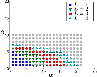
Figure 1: Index sets $\mathcal{I}(L)$ for $D=N=1$, according to equation (24).

Remark 8.

Theorem 1 is only valid in case Assumptions 1– 4 are true. In the next section we motivate these assumption for a specific elliptic problem that we use for numerically testing the MISC method. However, we stress that deriving bounds on the error and work contributions is problem-dependent and the corresponding analysis must be carried out in each case. Moreover, under a different set of assumption the complexity theorem would have to be rewritten accordingly.

5 Example and numerical evidence

In this section, we test the effectiveness of the MISC approximation on some instances of the general elliptic equation (3) in Example 1; more precisely, we consider a problem with one physical dimension ($d=1$) as well as a more challenging problem with three dimensions ($d=3$); in both cases, we set $\mathscr{B}=[0,1]^{d}$, $\mathscr{F}({{\bm{x}}})=1$. As for the random diffusion coefficient, we set

$$a({{\bm{x}}},{{\bm{y}}})=e^{\gamma_{N}({{\bm{x}}},{{\bm{y}}})},\quad\gamma_{N}({{\bm{x}}},{{\bm{y}}})=\sum_{n=1}^{N}\lambda_{n}\psi_{n}({{\bm{x}}})y_{n},$$ (28)

where $y_{n}$ are uniform random variables over $\Gamma_{n}=[-1,1]$, $\lambda_{n}=\sqrt{3}\exp(-n)$ and take $\psi_{n}$ to be a tensorization of trigonometric functions. More precisely, we define the function

$$\phi_{n}(x)=\begin{cases}\displaystyle\sin\left(\frac{n}{2}\pi x\right)&\text{if $n$ is even}\\[8.0pt] \displaystyle\cos\left(\frac{n-1}{2}\pi x\right)&\text{if $n$ is odd}\end{cases}$$

and set $\psi_{n}(x)=\phi_{n}(x)$ if $d=1$. If $d=3$, we take $\psi_{n}({{\bm{x}}})=\phi_{i(n)}(x_{1})\phi_{j(n)}(x_{2})\phi_{k(n)}(x_{3})$ for some indices ${i(n),j(n),k(n)}$ detailed in Table 1. Observe that the boundedness of the supports of the random variables $y_{n}$ guarantees the existence of the two bounding constants in equation (4), $a_{min}$ and $a_{max}$, that in turn assures the well posedness of the problem. Finally, the quantity of interest is defined as

$$F({{\bm{y}}})=\int_{\mathscr{B}}u({{\bm{x}}},{{\bm{y}}})Q({{\bm{x}}})d{{\bm{x}}},\quad Q({{\bm{x}}})=\frac{1}{(\sigma\sqrt{2\pi})^{d}}\exp\left(-\frac{\|{{\bm{x}}}-{{\bm{x}}}_{0}\|_{2}^{2}}{2\sigma^{2}}\right)$$ (29)

with $\sigma=0.16$ and locations ${{\bm{x}}}_{0}=0.3$ for $d=1$ and ${{\bm{x}}}_{0}=[0.3,0.2,0.6]$ for $d=3$. We also make the choice $h_{0}=1/3$ in Assumption 2. With these values and using the coarsest discretization, $h_{0}=1/3$, in all dimensions, the coefficient of variation of the quantity of interest can be approximated to be between $90\%$ and $100\%$ depending on the number of dimensions, $d$, and the number of random variables, $N$, that we consider below.

$n$	1	2	3	4	5	6	7	8	9	10
$i(n)$	1	2	1	1	3	2	2	1	1	1
$j(n)$	1	1	2	1	1	2	1	3	2	1
$k(n)$	1	1	1	2	1	1	2	1	2	3

Table 1: Included functions for $d=3$ in (28). Here $\psi_{n}({{\bm{x}}})=\phi_{i(n)}(x_{1})\phi_{j(n)}(x_{2})\phi_{k(n)}(x_{3})$.

5.1 Verifying bounds on work and error contributions

In this subsection we discuss the validity of Assumptions 2 to 4, upon which the MISC convergence theorem is based. To this end, we analyze separately the properties of the deterministic solver and of the collocation method applied to the problem just introduced.

Deterministic solver

The deterministic solver considered in this work consists of a tensorized finite difference solver, with the grid size along each direction, $x_{1},\ldots,x_{d}$, defined by $h_{i,\alpha_{i}}=h_{0}2^{-\alpha_{i}}$ and no other discretization parameters are considered: therefore, $D=d$, Assumption 2 is satisfied, and, due to the Dirichlet boundary conditions prescribed for $u$, the overall number of degrees of freedom of the corresponding finite difference solution is $\prod_{i=1}^{D}\left(\frac{1}{h_{i,\alpha_{i}}}-1\right)\leq\prod_{i=1}^{D}\left(\frac{1}{h_{i,\alpha_{i}}}\right)$. The associated linear system is solved with the GMRES method. We have numerically fitted the parameters, $\vartheta$ and $C_{\mathrm{GMRES}}$, in the model:

$${\mathrm{Work}\mspace{-2.0mu}\left[F_{{{\bm{\alpha}}}}\right]}\leq C_{\mathrm{GMRES}}\prod_{i=1}^{D}(h_{i,\alpha_{i}})^{-\vartheta},$$

for each individual tensor grid solve and found that $\vartheta=1$ gives a good fit in our numerical experiments. From this we can recover the rates $\{\tilde{\gamma}_{i}\}_{i=1}^{D}$ and the constant $C_{\mathrm{work}}^{\textnormal{det}}$ in (19) with the following argument: since computing ${{\bm{\Delta}}}^{\textnormal{det}}[F^{{{\bm{\alpha}}}}]$ requires up to $2^{D}$ solver calls, each on a different grid (cf. equation (11)), we have

$$\Delta W_{{{\bm{\alpha}}}}^{\textnormal{det}} ={\mathrm{Work}\mspace{-2.0mu}\left[{{\bm{\Delta}}}^{\textnormal{det}}[F_{{{\bm{\alpha}}}}]\right]}=\sum_{{{\bm{j}}}\in\{0,1\}^{D}}{\mathrm{Work}\mspace{-2.0mu}\left[F_{{{{\bm{\alpha}}}}-{{\bm{j}}}}\right]}$$

$$\leq C_{\mathrm{GMRES}}\sum_{{{\bm{j}}}\in\{0,1\}^{D}}\prod_{i=1}^{D}\left(h_{0}2^{-(\alpha_{i}-j_{i})}\right)^{-\vartheta}$$

$$=C_{\mathrm{GMRES}}\left(\prod_{i=1}^{D}\left(h_{0}2^{-\alpha_{i}}\right)^{-\vartheta}\right)\sum_{{{\bm{j}}}\in\{0,1\}^{D}}\prod_{i=1}^{D}2^{-j_{i}\vartheta}$$

$$=C_{\mathrm{GMRES}}(1+2^{-\vartheta})^{D}\prod_{i=1}^{D}(h_{i,\alpha_{i}})^{-\vartheta},$$

i.e., bound (19) is verified with $\widetilde{\gamma}_{i}=\vartheta,\forall i=1,\ldots,D$ and $C_{\mathrm{work}}^{\textnormal{det}}=C_{\mathrm{GMRES}}(1+2^{-\vartheta})^{D}$. Hence, the sum of costs of the solver calls is proportional to the cost of the call on the finest grid.

Concerning the error contribution $\Delta E_{{{\bm{\alpha}}}}^{\textnormal{det}}$, we observe numerically that bound (20) holds true in practice with $\widetilde{{r}}_{i}=2$, $i=1,\ldots,D$, due to the fact that $a\in C^{\infty}(\mathscr{B})$ for $\rho$-almost every ${{\bm{y}}}\in\Gamma$, $\mathscr{F}\in C^{\infty}(\mathscr{B})$ and the function $Q$ appearing in the quantity of interest (29) is also infinitely differentiable, confined in a small region inside the domain and zero up to machine precision on the boundary. In more detail, assuming for a moment that Assumption 3 is valid (we will numerically verify it later in this section), in Figure 2(a) we show the value of $\Delta E_{{{{\bm{\alpha}}}},{{{\bm{\beta}}}}}=\Delta E_{{{\bm{\alpha}}}}^{\textnormal{det}}\Delta E_{{{\bm{\beta}}}}^{\textnormal{stoc}}$ for fixed ${{{\bm{\beta}}}}=\bm{1}$ and variable ${{{\bm{\alpha}}}}=j\bar{{{{\bm{\alpha}}}}}+\bm{1},j=1,2,\ldots$, as well as the corresponding value of the bound (20) for $\Delta E_{{{\bm{\alpha}}}}^{\textnormal{det}}$. The line obtained by choosing $\bar{{{{\bm{\alpha}}}}}=[1,\,0,\,0]$ confirms that the size of $\Delta E_{{{\bm{\alpha}}}}^{\textnormal{det}}$ indeed decreases exponentially fast with respect to $\alpha_{1}$, and by fitting the computed values of $\Delta E_{{{\bm{\alpha}}}}^{\textnormal{det}}$ we obtain that the convergence rate is $\widetilde{{r}}_{j}=2$, as previously mentioned; analogous conclusions can be obtained for $\alpha_{2}$ and $\alpha_{3}$ by setting $\bar{{{{\bm{\alpha}}}}}=[0,\,1,\,0]$ (shown in Figure 2(a)) and $\bar{{{{\bm{\alpha}}}}}=[0,\,0,\,1]$ (not shown). Most importantly, confirmation of the product structure of $\Delta E_{{{\bm{\alpha}}}}^{\textnormal{det}}$ can be obtained by observing, e.g., the decay of $\Delta E_{{{\bm{\alpha}}}}^{\textnormal{det}}$ for $\bar{{{{\bm{\alpha}}}}}=[1,\,1,\,0]$ and $\bar{{{{\bm{\alpha}}}}}=[1,\,1,\,1]$.

(a) For fixed ${{{{\bm{\beta}}}}=\bm{1}}$ and variable ${{{{\bm{\alpha}}}}=k\bar{{{{\bm{\alpha}}}}}+\bm{1}}$.

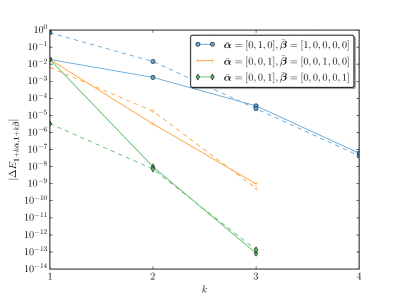
(b) For fixed ${{{{\bm{\alpha}}}}=\bm{1}}$ and variable ${{{{\bm{\beta}}}}=k\bar{{{{\bm{\beta}}}}}+\bm{1}}$.

Figure 2: Verifying the validity of the bound (23b) for the value of $|\Delta E_{{{{\bm{\alpha}}}},{{{\bm{\beta}}}}}|$ for the test case with $D=3$ and $N=5$. The dashed lines are based on the model in (23b) with ${\tilde{{r}}_{i}=2}$ for all $i=1,2,3$ and $g_{j}$ as in Table 2 for $j=1,\ldots,5$. The solid lines are based on computed values.

Stochastic discretization

The interpolation over the parameter space is based on the tensorized Lagrangian interpolation technique with Clenshaw-Curtis points explained in Section 2.1, cf. eqs. (5) and (6). In particular, due to the nestedness of the Clenshaw-Curtis points, adding the operator $\Delta^{\textnormal{stoc}}[F_{{{{\bm{\alpha}}}},{{{\bm{\beta}}}}}]$ to the MISC estimator will require $\Delta W_{{{\bm{\beta}}}}^{\textnormal{stoc}}=\prod_{j=1}^{N}\big{(}m(\beta_{j})-m(\beta_{j}-1)\big{)}$ new collocation points, which in view of equation (6) can be bounded as

$$m(\beta_{j})-m(\beta_{j}-1)=\begin{cases}1\mbox{ if }\beta_{j}=1\\ 2\mbox{ if }\beta_{j}=2\\ 2^{\beta_{j}-2},\mbox{ if }\beta_{j}>2,\end{cases}\leq 2^{\beta_{j}{-1}},\quad\forall j=1,2,\ldots,$$

provided that the set $\mathcal{I}$ is downward closed: Assumption 2 and bound (21) in Assumption 4 are thus verified. Observe that the nestedness of the Clenshaw-Curtis knots is a key property here: indeed, if the nodes are not nested $\Delta W_{{{\bm{\beta}}}}^{\textnormal{stoc}}$ is not uniquely defined, i.e., it depends on the set $\mathcal{I}$ to which $\Delta^{\textnormal{stoc}}[F_{{{{\bm{\alpha}}}},{{{\bm{\beta}}}}}]$ is being added, see, e.g., [34, Example 1 in Section 3].

Finally, to discuss the validity of bound (22) for $\Delta E_{{{\bm{\beta}}}}^{\textnormal{stoc}}$, we rely on the theory developed in our previous works [35, 34]. We begin by introducing the Chebyshev polynomials of the first kind $\Psi_{q}(y)$ for $y\in[-1,1]$, which are defined by the relation

$$\Psi_{q}(\cos(\theta))=\cos(q\theta),\quad 0\leq\theta\leq\pi,\quad q\in\mathbb{N}.$$

Then, for any multi-index ${{\bm{q}}}\in\mathbb{N}^{N}$, we consider the $N$-variate Chebyshev polynomials $\bm{\Psi}_{{\bm{q}}}({{\bm{y}}})=\prod_{n=1}^{N}\Psi_{q_{n}}(y_{n})$ and introduce the spectral expansion of $f:[-1,1]^{N}\rightarrow\mathbb{R}$ over $\{\bm{\Psi}_{{\bm{q}}}\}_{{{\bm{q}}}\in\mathbb{N}^{N}}$,

$$f({{\bm{y}}})=\sum_{{{\bm{q}}}\in\mathbb{N}^{N}}f_{{\bm{q}}}\bm{\Psi}_{{\bm{q}}}({{\bm{y}}}),\quad f_{{\bm{q}}}=\int_{\Gamma}f({{\bm{y}}})\bm{\Psi}_{{\bm{q}}}({{\bm{y}}})\prod_{n=1}^{N}\frac{1}{\sqrt{1-y_{n}^{2}}}d{{\bm{y}}},$$

Next, given any $\xi_{1},\xi_{2},\ldots,\xi_{N}>1$ we introduce the Bernstein polyellipse $\mathcal{E}_{\xi_{1},\ldots,\xi_{N}}=\prod_{n=1}^{N}\mathcal{E}_{n,\xi_{n}}$, where $\mathcal{E}_{n,\xi_{n}}$ denotes the ellipses in the complex plane defined as

$$\mathcal{E}_{n,\xi_{n}}=\bigg{\{}z_{n}\in\mathbb{C}:\,\,\real{z}\leq\frac{\xi_{n}+\xi_{n}^{-1}}{2}\cos{\phi},\,\,\,\mathfrak{Im}\left(z\right)\leq\frac{\xi_{n}-\xi_{n}^{-1}}{2}\sin{\phi},\,\,\phi\in[0,2\pi)\bigg{\}},$$

and recall the following lemma (see [34, Lemma 2] for a proof).

Lemma 1.

Let $f:[-1,1]^{N}\rightarrow\mathbb{R}$, and assume that there exist $\xi_{1},\xi_{2},\ldots,\xi_{N}>1$ such that $f$ admits a complex continuation $f^{*}:\mathbb{C}^{N}\rightarrow\mathbb{R}$ holomorphic in the Bernstein polyellipse $\mathcal{E}_{\xi_{1},\ldots,\xi_{N}}$ with $\sup_{{{\bm{z}}}\in\mathcal{E}_{\xi_{1},\ldots,\xi_{N}}}|f^{*}({{\bm{z}}})|\leq B$ and $B=B(\xi_{1},\xi_{2},\ldots,\xi_{n})<\infty$. Then $f$ admits a Chebyshev expansion that converges in $C^{0}([-1,1]^{N})$, and whose coefficients $f_{{\bm{q}}}$ are such that

$$|f_{{\bm{q}}}|\leq C_{\textnormal{Cheb}}({{\bm{q}}})\prod_{n=1}^{N}e^{-g^{*}_{n}q_{n}},\quad g^{*}_{n}=\log\xi_{n}$$ (30)

with $C_{\textnormal{Cheb}}({{\bm{q}}})=2^{\|{{\bm{q}}}\|_{0}}B$, where $\|{{\bm{q}}}\|_{0}$ denotes the number of non-zero elements of ${{\bm{q}}}$.

The following lemma then shows that the region of analyticity of $F({{\bm{y}}})$ indeed contains a Bernstein ellipse, so that a decay of exponential type can be expected for its Chebyshev coefficients.

Lemma 2.

The quantity of interest $F({{\bm{y}}})=\Theta[u(\cdot,{{\bm{y}}})]$ is analytic in a Bernstein polyellipse with parameters $\xi_{n}=\tau_{n}+\sqrt{\tau_{n}^{2}+1}$, for any $\tau_{n}<\frac{\pi}{2N\lambda_{n}}$.

Proof.

Equation (3) can be extended in the complex domain by replacing ${{\bm{y}}}$ with ${{\bm{z}}}\in\mathbb{C}^{N}$, and is analytic in the set $\Sigma=\left\{{{\bm{z}}}\in\mathbb{C}^{N}:\Re e{[a({{\bm{x}}},{{\bm{z}}})]}>0\right\}$, see, e.g., [6]. By writing $z_{n}=b_{n}+ic_{n}$, we have

$$a({{\bm{x}}},{{\bm{z}}}) =\exp\left(\sum_{n}z_{n}\lambda_{n}\psi_{n}({{\bm{x}}})\right)=\exp\left(\sum_{n}b_{n}\lambda_{n}\psi_{n}({{\bm{x}}})\right)\exp\left(\sum_{n}ic_{n}\lambda_{n}\psi_{n}({{\bm{x}}})\right)$$

$$=\exp\left(\sum_{n}b_{n}\lambda_{n}\psi_{n}({{\bm{x}}})\right)\left[\cos\left(\sum_{n}c_{n}\lambda_{n}\psi_{n}({{\bm{x}}})\right)+i\sin\left(\sum_{n}c_{n}\lambda_{n}\psi_{n}({{\bm{x}}})\right)\right]$$

so that the region $\Sigma$ can be rewritten as

$$\Sigma=\left\{{{\bm{z}}}={{\bm{b}}}+i{{\bm{c}}}\in\mathbb{C}^{N}:\cos\left(\sum_{n}c_{n}\lambda_{n}\psi_{n}({{\bm{x}}})\right)>0,\forall{{\bm{x}}}\in\mathscr{B}\right\}.$$

Such a region includes the smaller region

$$\Sigma_{2}=\left\{{{\bm{z}}}={{\bm{b}}}+i{{\bm{c}}}\in\mathbb{C}^{N}:\left\|\sum_{n}c_{n}\lambda_{n}\psi_{n}\right\|_{L^{\infty}(\mathscr{B})}<\frac{\pi}{2}\right\},$$

which in turn includes

$$\Sigma_{3}=\left\{{{\bm{z}}}={{\bm{b}}}+i{{\bm{c}}}\in\mathbb{C}^{N}:\sum_{n}\lambda_{n}|c_{n}|<\frac{\pi}{2}\right\},$$

where the last equality is due to the fact that, by construction, $\left\|\psi_{n}\right\|_{L^{\infty}(\mathscr{B})}=1$, cf. equation (28). Next we let $\tau_{n}=\frac{\pi}{2N\lambda_{n}}$ and define the following subregion of $\Sigma_{3}$:

$$\Sigma_{4}=\bigg{\{}{{\bm{z}}}={{\bm{b}}}+i{{\bm{c}}}\in\mathbb{C}^{N}:|c_{n}|<\tau_{n}\bigg{\}}\subset\Sigma_{3}.$$

$\Sigma_{4}$ is actually a polystrip in the complex plain that it in turn contains the Bernstein ellipse with parameters $\xi_{n}$ such that

$$\frac{\xi_{n}-\xi_{n}^{-1}}{2}=\tau_{n}\Rightarrow\xi_{n}^{2}-1-2\tau_{n}\xi_{n}=0\Rightarrow\xi_{n}=\tau_{n}+\sqrt{\tau_{n}^{2}+1}$$

in which $u({{\bm{x}}},{{\bm{y}}})$ is analytic. Finally, the quantity of interest, $F=\Theta[u]$, is also analytic in the same Bernstein polyellipse due to the linearity of the operator $\Theta$. ∎

Remark 9.

Incidentally, we remark that the choice of $\tau_{n}$ considered in Lemma 2 degenerates for $N\to\infty$. In this case, if we know that $\sum_{n=0}^{\infty}(\lambda_{n}\|\psi_{n}\|_{L^{\infty}(\mathscr{B})})^{p}<\infty$ for some $p<1$, then we could set $\tau_{n}=\frac{\pi}{2}(\lambda_{n}\|\psi_{n}\|_{L^{\infty}(\mathscr{B})})^{p-1}$, which does not depend on $N$.

Lemma 3.

$$\Delta E_{{{\bm{\beta}}}}^{\textnormal{stoc}}\leq C_{E}e^{-\sum_{n=1}^{N}g^{*}_{n}m(\beta_{n}-1)}\mathbb{M}^{m({{{\bm{\beta}}}})}$$ (31)

holds, where $C_{E}=4^{N}B\prod_{n=1}^{N}\frac{1}{1-e^{-g^{*}_{n}}}$, $B$ as in Lemma 1, $g^{*}_{n}=\log\xi_{n}$ with $\xi_{n}$ as in Lemma 2, and $\mathbb{M}^{m({{{\bm{\beta}}}})}$ has been defined in equation (7).

Proof.

Combining Lemmas 1 and 2, we obtain that the Chebyshev coefficients of $F$ can be bounded as

$$|F_{{\bm{q}}}|\leq C_{\textnormal{Cheb}}({{\bm{q}}})\prod_{n=1}^{N}e^{-g^{*}_{n}q_{n}},$$

with $g^{*}_{n}=\log\xi_{n}=\log(\tau_{n}+\sqrt{\tau_{n}^{2}+1})$ and $\tau_{n}$ as in Lemma 2. Then, the result can be obtained following the same argument of [34, Lemma 5]. ∎

To conclude, we first observe that $\mathbb{M}^{m({{{\bm{\beta}}}})}$ grows logarithmically with respect to $m({{{\bm{\beta}}}})$, see eq. (8), so it is asymptotically negligible in the estimate above, i.e. we can write

$$\Delta E_{{{\bm{\beta}}}}^{\textnormal{stoc}}\leq C_{E_{2}}(\epsilon)\prod_{n=1}^{N}e^{-g^{*}_{n}(1-\epsilon_{E})m(\beta_{n}-1)}$$

for an arbitrary $\epsilon_{E}>0$ and with $C_{E_{2}}(\epsilon_{E})>C_{E}$, and furthermore that the definition of $m(i)$ in (6) implies that $m(i-1)\geq\frac{m(i)-1}{2}$. We can finally write

$$\Delta E_{{{\bm{\beta}}}}^{\textnormal{stoc}} \leq C_{E_{2}}(\epsilon)\prod_{n=1}^{N}e^{-g^{*}_{n}(1-\epsilon_{E})\frac{m(\beta_{n})-1}{2}}=C_{\mathrm{error}}^{\textnormal{stoc}}\prod_{n=1}^{N}e^{-\widetilde{g}_{n}m(\beta_{n})},$$

with $C_{\mathrm{error}}^{\textnormal{stoc}}=C(\epsilon)\prod_{n=1}^{N}e^{\frac{g^{*}_{n}}{2}(1-\epsilon)}$ and $\widetilde{g}_{n}=\frac{g^{*}_{n}}{2}(1-\epsilon_{E})$. The latter bound actually shows that bound (22) in Assumption 4 is valid for the test we are considering. Finally, we point out that in practice we work with the expression (23b), whose rates $g_{n}$ are actually better estimated numerically, using the same procedure used to obtain the deterministic rates $\tilde{{r}}_{j}=2$: we choose a sufficiently fine spatial resolution level ${{{\bm{\alpha}}}}$, consider a variable ${{{\bm{\beta}}}}=j\bar{{{{\bm{\beta}}}}}+\bm{1}$ and fit the (simplified) model $\Delta E_{{{\bm{\beta}}}}^{\textnormal{stoc}}\leq C\prod_{n=1}^{N}e^{-g_{n}2^{\beta_{n}}}$. The values obtained are reported in Table 2, and they are found to be equal for the case $d=1$ and $d=3$ (see also [52, 35, 8]). To make sure that the estimated value of $g_{n}$ does not depend on the spatial discretization, one could repeat the procedure for a few different values of ${{{\bm{\alpha}}}}$ and verify that the estimate is robust with respect to the spatial discretization: we note, however, that a rough estimate of $g_{n}$ will also be sufficient, since the convergence of the method is in practice dictated by the deterministic solver, as we have already discussed in Remark 7. Figure 2(b) then shows the validity of the bound $\Delta E_{{{\bm{\beta}}}}^{\textnormal{stoc}}\leq C\prod_{n=1}^{N}e^{-g_{n}2^{\beta_{n}}}$ comparing for fixed ${{{\bm{\alpha}}}}=\bm{1}$ and ${{{\bm{\beta}}}}=j\bar{{{{\bm{\beta}}}}}+\bm{1}$ the value of $\Delta E_{{{{\bm{\alpha}}}}}^{\textnormal{det}}\Delta E_{{{\bm{\beta}}}}^{\textnormal{stoc}}$ and the corresponding estimate.

	$g_{1}$	$g_{2}$	$g_{3}$	$g_{4}$	$g_{5}$	$g_{6}$	$g_{7}$	$g_{8}$	$g_{9}$	$g_{10}$
	2.4855	2.8174	4.5044	4.1938	4.7459	6.8444	7.1513	7.8622	8.6584	9.4545

Table 2: Values of rates $g$ for the test cases considered.

Stochastic-deterministic product structure

We conclude this section by verifying Assumption 3, i.e., the fact that the error contribution can be factorized as $\Delta E_{{{{\bm{\alpha}}}},{{{\bm{\beta}}}}}=\Delta E_{{{\bm{\alpha}}}}^{\textnormal{det}}\Delta E_{{{\bm{\beta}}}}^{\textnormal{stoc}}$ and that an analogous decomposition holds for $\Delta W_{{{{\bm{\alpha}}}},{{{\bm{\beta}}}}}$. While the latter is trivial, to verify the former we employ the same strategy used to verify the models for $\Delta E_{{{\bm{\alpha}}}}^{\textnormal{det}}$ and $\Delta E_{{{\bm{\beta}}}}^{\textnormal{stoc}}$, this time letting both ${{{\bm{\alpha}}}}$ and ${{{\bm{\beta}}}}$ change for every point, i.e., ${{{\bm{\alpha}}}}=j\bar{{{{\bm{\alpha}}}}}+\bm{1}$ and ${{{\bm{\beta}}}}=j{{{\bm{\beta}}}}_{0}+\bm{1}$. Figure 3 shows the comparison between the computed value of $\Delta E_{{{{\bm{\alpha}}}},{{{\bm{\beta}}}}}$ and their estimated counterpart and confirms the validity of the product structure assumption.

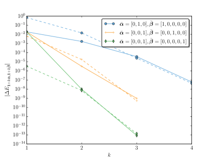
Figure 3: Comparison of $|\Delta E_{{{{\bm{\alpha}}}},{{{\bm{\beta}}}}}|$ for ${{{\bm{\beta}}}}=j\bar{{{{\bm{\beta}}}}}+\bm{1}$ and ${{{\bm{\alpha}}}}=j\bar{{{{\bm{\alpha}}}}}+\bm{1}$ for the test case with $D=3$ and $N=5$. The dashed lines are based on the model in (23b) with ${\tilde{{r}}_{i}=2}$ for all $i=1,2,3$ and $g_{j}$ as in Table 2 for $j=1,\ldots,5$. The solid lines are based on computed values.

5.2 Test setup

In our numerical tests, we compare MISC with the methods listed below. For each of them we show (for both test cases considered) plots of the convergence of the error in the computation of ${\mathbb{E}\mspace{-2.0mu}\left[F\right]}$ with respect to the computational work, taking as a reference value the result obtained using a well-resolved MISC solution. To avoid discrepancies in running time due to implementation details, the computational work is estimated in terms of the total number of degrees of freedom, i.e., using (14) and (23a). The names used here for the methods are also used in the legends of the figures showing the convergence plots.

“a-priori” MISC

refers to the MISC method with index set $\mathcal{I}$ defined by (17), where $\Delta W_{{{{\bm{\alpha}}}},{{{\bm{\beta}}}}}$ and $\Delta E_{{{{\bm{\alpha}}}},{{{\bm{\beta}}}}}$ are taken to equal their upper bounds in (23a) and (23b), respectively. The resulting set is explicitly written in (24). The convergence rate of this set is predicted by Theorem 1, cf. Remark 6. Note that we do not need to determine the value of the constants $C_{\text{{work}}}$ and $C_{\text{{error}}}$ since they can be absorbed in the parameter $\epsilon$ in (17).

“a-posteriori” MISC

refers to the MISC method with index set $\mathcal{I}$ defined by (17), where $\Delta W_{{{{\bm{\alpha}}}},{{{\bm{\beta}}}}}$ is taken to equal its upper bound in (23a), and $\Delta E_{{{{\bm{\alpha}}}},{{{\bm{\beta}}}}}$ is instead computed explicitly as $\left|\Delta[F_{\alpha,\beta}]\right|$. Notice that this method is not practical since the cost of constructing set $\mathcal{I}$ would dominate the cost of the MISC estimator by far. However, this method would produce the best possible convergence and serve as a benchmark for both “a-priori” MISC and the bound (23b).

MLSC

(only in the case $d>1$) refers to the Multilevel Stochastic Collocation obtained by setting $\alpha_{1}=\ldots=\alpha_{D}$ (i.e. considering the mesh-size as the only discretization parameter), as already mentioned in Remark 5; we recall this is not exactly the MLSC method that was implemented in [24], see again Remark 5. Just as with MISC, we consider both the “a-priori” and “a-posteriori” version of MLSC, where $\Delta E_{{{{\bm{\alpha}}}},{{{\bm{\beta}}}}}$ is taken to be equal to its upper (23b) in the former case and assessed by direct numerical evaluation in the latter case.

SCC

refers to the “Sparse Composite Collocation method” in Remark 5, see equation (18).

MIMC

refers to the Multi-Index Monte Carlo method as detailed in [29], for which the complexity ${\mathcal{O}\left(W_{\max}^{-0.5}\right)}$ can be estimated for the test case at hand and as long as $d<4$.

SGSC

refers to the quasi-optimal Sparse Grids Stochastic Collocation (SGSC) with fixed spatial discretization as proposed in [35, 34]. To determine the needed spatial discretization for a given work and for a fair comparison against MISC, we actually compute the convergence curves of SGSC for all relevant levels of spatial discretizations and then show in the plots only the lower envelope of the corresponding convergence curves, ignoring the possible spurious reductions of error that might happen due to non-asymptotic, unpredictable cancellations, cf. Figure 4. In this way, we ensure that the error shown for such “single-level methods” has been obtained with the smallest computational error possible. Again, this is not a computationally practical method but is taken as a reference for what a sparse grids Stochastic Collocation method with optimal balancing of the space and stochastic discretization errors could achieve.

Figure 4: Envelope of SGSC convergence curves for the test case with $d=3$ and $N=10$.

5.3 Implementation details

To implement MISC, we need two components:

1. Given a profit level parameter, $\epsilon$, we build the quasi-optimal set $\mathcal{I}$ based on (17), (23a) and (23b). One method to achieve this is to exploit the fact that this set is downward closed and use the following recursive algorithm.

   FUNCTION BuildSet(epsilon, multiIndex)
       FOR i = 1 to (D+N)
           IF Profit(multiIndex + e_i) > epsilon
           THEN
               ADD multiIndex+e_i to FinalSet
               CALL BuildSet(epsilon, multiIndex+e_i)
           END IF
       END FOR
   END FUNCTION
     
   

2. Given the set, $\mathcal{I}(L)$, we evaluate (13). Here we have two choices:

   • Evaluate the individual terms ${{\bm{\Delta}}}[F_{{{{\bm{\alpha}}}},{{{\bm{\beta}}}}}]$ for every ${{{\bm{\alpha}}}},{{{\bm{\beta}}}}\in\mathcal{I}$. To do so, we use the operator defined in (9) along each stochastic and spatial direction. By storing the values of these terms, we can evaluate the MISC with different index sets (contained in $\mathcal{I}(L)$), which might be required to test the convergence of the MISC method. Moreover, this implementation is suitable for adaptive methods that expand the index set based on some criteria and reevaluate the MISC estimator. On the other hand, this implementation has a computational overhead since most computed values of $F_{{{{\bm{\alpha}}}},{{{\bm{\beta}}}}}$ will actually not contribute to the final value of the estimator. However, this computational overhead is only a fraction of the minimum time required to evaluate the estimator.

   • Use the combination form of (13) and only compute the terms that have $c_{{{{\bm{\alpha}}}},{{{\bm{\beta}}}}}\neq 0$. This would remove the overhead of computing terms that make zero contribution to the estimator. This implementation is more efficient but less flexible as we cannot evaluate the estimator on sets contained in $\mathcal{I}(L)$ or build the set adaptively.

5.4 Test with $D=1$

Here we consider three different numbers of stochastic variables, namely $N=1,5,10$. Results are shown in Figure 5. As expected, a-posteriori MISC shows the best convergence, with a-priori MISC being slightly worse and the single level methods following. Finally, we verify the accuracy of the estimated asymptotic convergence rate provided by Theorem 1: in this case, $\zeta=\frac{{r}_{1}}{\gamma_{1}}=\frac{\widetilde{{r}}_{1}\log 2}{\widetilde{\gamma}_{1}\log 2}=2$ and $\mathfrak{z}=1$ holds. Hence, the predicted convergence rate is $W^{-\zeta}(\log W)^{(\zeta+1)(\mathfrak{z}-1)}=W^{-2}$, which appears to be in good agreement with the experimental convergence rate.

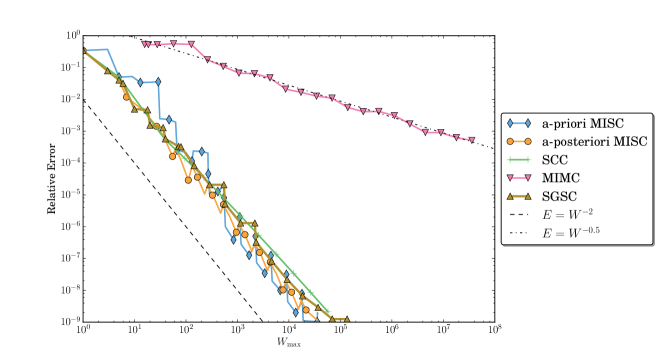
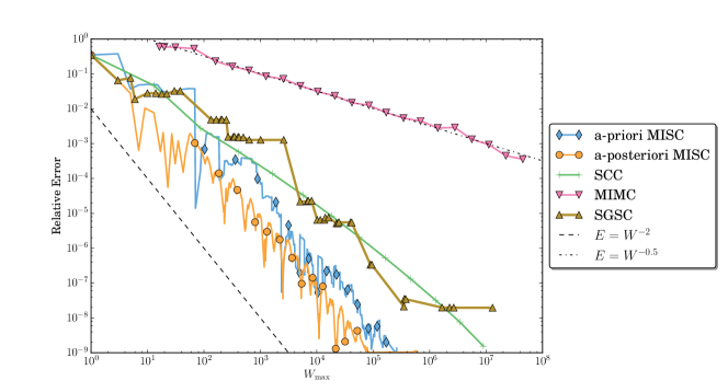
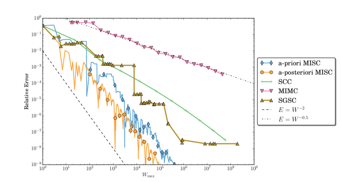
Figure 5: Results for test $D=1$, case $N=1$ (top), $N=5$ (center) and $N=10$ (bottom).

5.5 Test with $D=3$

In this case, we obtain the convergence curves shown in Figure 6, where the Multilevel Stochastic Collocation method has also been included. The hierarchy between the methods is in agreement with the case $d=1$, with the Multilevel Stochastic Collocation being comparable or slightly better than single level methods, but worse than the MISC approaches as expected.

Concerning the accuracy of the theoretical estimate: since for this test $\widetilde{{r}}_{1}=\widetilde{{r}}_{2}=\widetilde{{r}}_{2}=2$ and $\widetilde{\gamma}_{1}=\widetilde{\gamma}_{2}=\widetilde{\gamma}_{3}=1$, $\zeta=2$ still holds, while this time $\mathfrak{z}=3$; hence, the predicted convergence rate is $W^{-\zeta}(\log W)^{(\zeta+1)(\mathfrak{z}-1)}=W^{-2}(\log W)^{6}$. The plots suggest that the theoretical estimates might be slightly too optimistic when $N$ increases but it is important to recall that Theorem 1 gives only an asymptotic result, and the plot could be negatively influenced by pre-asymptotic effects. Observe also that in this case there are a few data points where a-posteriori MISC is not better than a-priori MISC; this observation can be ascribed to the fact that a-posteriori MISC is optimal only with respect to the upper bound in (3.1). In other words, a-posteriori MISC selects the contributions according to the absolute value of the contributions but then the MISC estimator is computed by summing signed contributions. Hence, cancellations between contributions with similar sizes and opposite signs will occur.

Finally, we remark that, in our calculations, MLSC and SGSC were not able to achieve very small errors, unlike MISC. This is due to a limitation in the linear solver we are using that allows systems with only up to $2^{17}$ degrees of freedom (around 1GB of memory) to be solved. These “single-level” methods hit that limit sooner than MISC since they entail solving a very large system that comes from isotropically discretizing all three spatial dimensions.

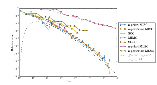
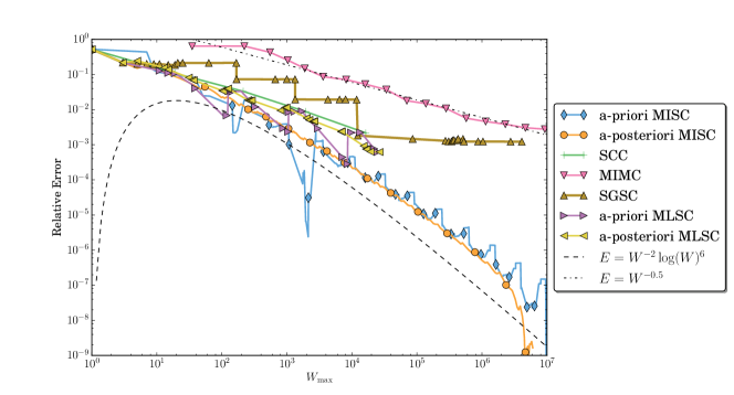
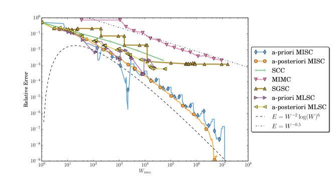
Figure 6: Results for test $D=3$, case $N=1$ (top), $N=5$ (center) and $N=10$ (bottom).

6 Conclusions

In this work, we have proposed MISC, a combination technique method to solve UQ problems, optimizing both the deterministic and stochastic resolution levels simultaneously to minimize the computational cost. A distinctive feature of MISC is that its construction is based on the notion of profit of the mixed differences composing it, rather than balancing the total error contributions arising from the deterministic and stochastic components. We have detailed a complexity analysis and derived a convergence theorem showing that in certain cases the convergence of the method is essentially dictated by the convergence properties of the deterministic solver. We have then verified the effectiveness of the method proposed on a couple of numerical test cases, comparing its performance with other methods available in the literature. The results obtained are encouraging, as they suggest that the proposed methodology is more effective than the other methods considered here. The theoretical results have been also found to be consistent with the numerical results to a satisfactory extent.

As a final remark, we observe that the methodology presented here is not limited to the spatial or temporal discretization parameters of the deterministic problem, but could also be applied to other discretization parameters, such as smoothing parameters or artificial viscosities.

Acknowledgement

F. Nobile and L. Tamellini received support from the Center for ADvanced MOdeling Science (CADMOS) and partial support by the Swiss National Science Foundation under the Project No. 140574 “Efficient numerical methods for flow and transport phenomena in heterogeneous random porous media”. R. Tempone is a member of the KAUST Strategic Research Initiative, Center for Uncertainty Quantification in Computational Sciences and Engineering.

Appendix A Proof of Theorem 1

The following technical lemmas are needed in the convergence proof.

Lemma 4.

For ${{\bm{x}}}\in(1,\infty)^{D}$, define $\lfloor{{\bm{x}}}\rfloor=\left(\lfloor x_{i}\rfloor\right)_{i=1}^{D}$. For any $f:(1,\infty)^{D}\to\mathbb{R}$ and $g:(1,\infty)^{D}\to\mathbb{R}_{+}$,

$$\sum_{\{{{{\bm{\alpha}}}}\in\mathbb{N}_{+}^{D}\>:\>f({{{\bm{\alpha}}}})\leq 0\}}g({{{\bm{\alpha}}}})=\int_{\{{{\bm{x}}}\in(1,\infty)^{D}\>:\>f(\lfloor{{\bm{x}}}\rfloor)\leq 0\}}g(\lfloor{{\bm{x}}}\rfloor)~{}\text{d}{{\bm{x}}}$$

holds. Moreover, if $g$ and $f$ are increasing, then

$$\sum_{\{{{{\bm{\alpha}}}}\in\mathbb{N}_{+}^{D}\>:\>f({{{\bm{\alpha}}}})\leq 0\}}g({{{\bm{\alpha}}}})\leq\int_{\{{{\bm{x}}}\in(1,\infty)^{D}\>:\>f({{\bm{x}}}-1)\leq 0\}}g({{\bm{x}}})~{}\text{d}{{\bm{x}}},$$

and if $g$ and $f$ are decreasing, then

$$\sum_{\{{{{\bm{\alpha}}}}\in\mathbb{N}_{+}^{D}\>:\>f({{{\bm{\alpha}}}})\leq 0\}}g({{{\bm{\alpha}}}})\leq\int_{\{{{\bm{x}}}\in(1,\infty)^{D}\>:\>f({{\bm{x}}})\leq 0\}}g({{\bm{x}}}-1)~{}\text{d}{{\bm{x}}}.$$

Proof.

We have

$$\sum_{\{{{{\bm{\alpha}}}}\in\mathbb{N}_{+}^{D}\>:\>f({{{\bm{\alpha}}}})\leq 0\}}g({{{\bm{\alpha}}}}) =\sum_{\{{{{\bm{\alpha}}}}\in\mathbb{N}_{+}^{D}\>:\>f({{{\bm{\alpha}}}})\leq 0\}}g({{{\bm{\alpha}}}})\int_{{{\bm{x}}}\in[0,1]^{D}}~{}\text{d}{{\bm{x}}}$$

$$=\sum_{\{{{{\bm{\alpha}}}}\in\mathbb{N}_{+}^{D}\>:\>f({{{\bm{\alpha}}}})\leq 0\}}\int_{{{\bm{x}}}\in[0,1]^{D}}g(\lfloor{{{\bm{\alpha}}}}+{{\bm{x}}}\rfloor)~{}\text{d}{{\bm{x}}}$$

$$=\int_{\{{{\bm{x}}}\in(1,\infty)^{D}\>:\>f(\lfloor{{\bm{x}}}\rfloor)\leq 0\}}g(\lfloor{{\bm{x}}}\rfloor)~{}\text{d}{{\bm{x}}}.$$

Combining these inequalities with $x-1\leq\lfloor x\rfloor\leq x$ finishes the proof. ∎

Lemma 5.

Assume ${{\bm{a}}}\in\mathbb{R}_{+}^{D}$, ${{\bm{b}}}\in\mathbb{R}_{+}^{D}$ and $L>|{{\bm{a}}}|$. Then,

$$\sum_{\{{{\bm{x}}}\in\mathbb{N}_{+}^{D}\>:\>\sum_{i=1}^{D}a_{i}e^{b_{i}x_{i}}+b_{i}x_{i}>L\}}\exp\left(-\sum_{i=1}^{D}a_{i}e^{b_{i}x_{i}}\right)\leq\left(\prod_{i=1}^{D}\frac{\exp(2a_{i})}{a_{i}^{2}}\right)\exp\left(-L\right)(L+1)^{2D+1}.$$

Proof.

Define the set

$$\mathcal{P}=\left\{\left(e^{b_{i}x_{i}}\right)_{i=1}^{D}\>:\>{{\bm{x}}}\in\mathbb{N}_{+}^{D}\right\},$$

and define $\lfloor{{\bm{y}}}\rfloor=\left(\lfloor y_{i}\rfloor\right)_{i=1}^{D}$. Then

$$\sum_{\{{{\bm{x}}}\in\mathbb{N}_{+}^{D}\>:\>\sum_{i=1}^{D}a_{i}e^{b_{i}x}+b_{i}x_{i}>L\}}\exp\left(-\sum_{i=1}^{D}a_{i}e^{b_{i}x_{i}}\right) =\sum_{\{{{\bm{y}}}\in\mathcal{P}\>:\>{{\bm{a}}}\cdot{{\bm{y}}}+|\log({{\bm{y}}})|>L\}}\exp(-{{\bm{a}}}\cdot{{\bm{y}}})$$

$$\leq\sum_{\{{{\bm{y}}}\in\mathcal{P}\>:\>{{\bm{a}}}\cdot(\lfloor{{\bm{y}}}\rfloor+{{\bm{1}}})+|\log(\lfloor{{\bm{y}}}\rfloor+{{\bm{1}}})|>L\}}\exp(-{{\bm{a}}}\lfloor{{\bm{y}}}\rfloor)$$

$$\leq\sum_{\{{{\bm{y}}}\in\mathbb{N}_{+}^{D}\>:\>{{\bm{a}}}\cdot{{\bm{y}}}+|\log({{\bm{y}}}+{{\bm{1}}})|>L-|{{\bm{a}}}|\}}\exp(-{{\bm{a}}}\cdot{{\bm{y}}})$$

$$\leq\int_{\{{{\bm{y}}}\in(1,\infty)^{D}\>:\>{{\bm{a}}}\cdot{{\bm{y}}}+|\log({{\bm{y}}}+{{\bm{1}}})|>L-|{{\bm{a}}}|\}}\exp(-{{\bm{a}}}\cdot({{\bm{y}}}-{{\bm{1}}}))~{}\text{d}{{\bm{y}}}.$$

Letting $z_{i}=a_{i}y_{i}+\log(y_{i}+1)$ and $p(z_{i})=y_{i}\leq\frac{z_{i}}{a_{i}}$, then

$$\sum_{\{{{\bm{x}}}\in\mathbb{N}_{+}^{D}\>:\>\sum_{i=1}^{D}a_{i}e^{b_{i}x}+b_{i}x_{i}>L\}}\exp{\left(-\sum_{i=1}^{D}a_{i}e^{b_{i}x_{i}}\right)}$$

$$=\exp(|{{\bm{a}}}|)\int_{\{{{\bm{y}}}\in(1,\infty)^{D}\>:\>{{\bm{a}}}\cdot{{\bm{y}}}+|\log({{\bm{y}}}+{{\bm{1}}})|>L-|{{\bm{a}}}|\}}\exp(-{{\bm{a}}}\cdot{{\bm{y}}}-|\log({{\bm{y}}}+{{\bm{1}}})|+|\log({{\bm{y}}}+{{\bm{1}}})|)~{}\text{d}{{\bm{y}}}$$

$$=\exp(|{{\bm{a}}}|)\int_{\{{{\bm{z}}}\in\otimes_{i=1}^{D}(a_{i}+\log(2),\infty)\>:\>|{{\bm{z}}}|>L-|{{\bm{a}}}|\}}\exp(-|{{\bm{z}}}|)\prod_{i=1}^{D}\left(\frac{p(z_{i})+1}{a_{i}+\frac{1}{p(z_{i})+1}}\right)~{}\text{d}{{\bm{z}}}$$

$$\leq\exp(|{{\bm{a}}}|)\int_{\{{{\bm{z}}}\in\otimes_{i=1}^{D}(a_{i}+\log(2),\infty)\>:\>|{{\bm{z}}}|>L-|{{\bm{a}}}|\}}\exp(-|{{\bm{z}}}|)\prod_{i=1}^{D}\left(\frac{z_{i}+a_{i}}{a_{i}^{2}}\right)~{}\text{d}{{\bm{z}}}$$

$$\leq\left(\prod_{i=1}^{D}\frac{\exp(a_{i})}{a_{i}^{2}}\right)\int_{\{{{\bm{z}}}\in\otimes_{i=1}^{D}(a_{i}+\log(2),\infty)\>:\>|{{\bm{z}}}|>L-|{{\bm{a}}}|\}}\exp(-|{{\bm{z}}}|+|\log({{\bm{z}}}+{{\bm{a}}})|)~{}\text{d}{{\bm{z}}}$$

$$=\left(\prod_{i=1}^{D}\frac{\exp(2a_{i})}{a_{i}^{2}}\right)\int_{\{{{\bm{x}}}\in\otimes_{i=1}^{D}(\log(2),\infty)\>:\>|{{\bm{x}}}|>L\}}\exp(-|{{\bm{x}}}|+|\log({{\bm{x}}})|)~{}\text{d}{{\bm{x}}}$$

$$\leq\left(\prod_{i=1}^{D}\frac{\exp(2a_{i})}{a_{i}^{2}}\right)\int_{\{{{\bm{z}}}\in\otimes_{i=1}^{D}(0,\infty)\>:\>|{{\bm{z}}}|>L\}}\exp(-|{{\bm{z}}}|+|\log({{\bm{z}}})|)~{}\text{d}{{\bm{z}}}.$$

Now let us prove, by induction on $D$, that we have

$$\int_{\{{{\bm{z}}}\in\mathbb{R}_{+}^{D}\>:\>|{{\bm{z}}}|>L\}}\exp(-|{{\bm{z}}}|+|\log({{\bm{z}}})|)~{}\text{d}{{\bm{z}}}\leq\exp(-L)(L+1)^{2D-1}\,\,.$$

For $D=1$, the inequality is a trivial equality that can be obtained with integration by parts. Assume the inequality is true for $D$ and let us prove it for $D+1$:

$$\int_{\{{{\bm{z}}}\in\mathbb{R}_{+}^{D+1}\>:\>|{{\bm{z}}}|>L\}}\exp(-|{{\bm{z}}}|+\log({{\bm{z}}}))~{}\text{d}{{\bm{z}}} =\int_{L}^{\infty}y\exp(-y)\int_{\{{{\bm{x}}}\in\mathbb{R}_{+}^{D}\}}\exp(-|{{\bm{x}}}|+\log({{\bm{x}}}))~{}\text{d}{{\bm{x}}}~{}\text{d}y$$

$$+\int_{0}^{L}y\exp(-y)\int_{\{{{\bm{x}}}\in\mathbb{R}_{+}^{D}\>:\>|{{\bm{x}}}|>L-y\}}\exp(-|{{\bm{x}}}|+\log({{\bm{x}}}))~{}\text{d}{{\bm{x}}}~{}\text{d}y$$

$$\leq\exp(-L)(L+1)$$

$$+\int_{0}^{L}y\exp(-y)\exp(-L+y)(L-y+1)^{2D-1}~{}\text{d}y$$

$$\leq\exp(-L)\left(L+1+L^{2}(L+1)^{2D-1}\right)$$

$$\leq\exp(-L)\left(L+1\right)\left(1+L(L+1)^{2D-1}\right)$$

$$\leq\exp(-L)(L+1)^{2(D+1)-1}\,\,.$$

Finally, substituting back, we get the result. ∎

Definition 1.

Given ${{\bm{a}}}\in\mathbb{R}_{+}^{D}$ and $A>0$, let $\mathfrak{n}({{\bm{a}}},A)$ denote the number of occurrences of $A$ in ${{\bm{a}}}$,

$$\mathfrak{n}({{\bm{a}}},A)=\#\{i=1,\ldots,d\>:\>a_{i}=A\}.$$

Lemma 6.

Assume $k\in\mathbb{N}$, ${{\bm{a}}}\in\mathbb{R}_{+}^{D},L>|{{\bm{a}}}|$. Then, the following bounds hold true:

$$\int_{\{{{\bm{x}}}\in\mathbb{R}_{+}^{D}\>:\>|{{\bm{x}}}|>L\}}\exp(-{{\bm{a}}}\cdot{{\bm{x}}})~{}\text{d}{{\bm{x}}}\leq\mathfrak{B}_{D}({{\bm{a}}})\exp(-\min({{\bm{a}}})L)L^{\mathfrak{n}({{\bm{a}}},\min({{\bm{a}}}))-1}$$

where $\mathfrak{B}_{D}({{\bm{a}}})$ is a positive constant independent of $L$.

Proof.

See [29, Lemma B.3] for a proof of the inequality and the value of $\mathfrak{B}_{D}({{\bm{a}}})$. Moreover, a proof of a consistent equality for the case ${{\bm{a}}}={{\bm{1}}}$ can be found in [51, Proposition 2.3]. ∎

Lemma 7.

Assume $k\in\mathbb{N}$, ${{\bm{a}}}\in\mathbb{R}_{+}^{D},L>|{{\bm{a}}}|$. Then, the following bound holds:

$$\int_{\{{{\bm{x}}}\in\mathbb{R}_{+}^{D}\>:\>|{{\bm{x}}}|\leq L\}}\exp\left({{\bm{a}}}\cdot{{\bm{x}}}\right)\left(L-|{{\bm{x}}}|\right)^{k}~{}\text{d}{{\bm{x}}}\leq\mathfrak{A}_{D}({{\bm{a}}},k)\exp(\max({{\bm{a}}})L)L^{\mathfrak{n}({{\bm{a}}},\max({{\bm{a}}}))-1},$$

where

$$\mathfrak{A}_{D}({{\bm{a}}},k)=\frac{k!}{(\mathfrak{n}({{\bm{a}}},\max({{\bm{a}}}))-1)!\max({{\bm{a}}})^{k+1}}\left(\prod_{a_{i}<\max({{\bm{a}}})}\frac{1}{\max({{\bm{a}}})-a_{i}}\right).$$

Proof.

Without loss of generality, assume that $a_{i}\geq a_{i+1}$ for all $i=1\ldots D$, such that $a_{1}=\max({{\bm{a}}})$. We prove the result by induction on $D$. For $D=1$, we have

$$\int_{0}^{L}\exp\left(ax\right)\left(L-x\right)^{k}~{}\text{d}x =\frac{k!}{a^{k+1}}\left(\exp(aL)-\sum_{i=0}^{k}\frac{a^{i}L^{i}}{i!}\right)$$

$$\leq\frac{k!\exp(aL)}{a^{k+1}}.$$

Next, assume that the result is valid for a given $D>1$ and ${{\bm{a}}}\in\mathbb{R}_{+}^{D}$ where $a_{i}\geq a_{i+1}$ for all $i=1\ldots D$, such that $a_{1}=\max({{\bm{a}}})$. Let $b\leq a_{1}$ and define a new vector $\widetilde{{{\bm{a}}}}=({{\bm{a}}},b)\in\mathbb{R}_{+}^{D+1}$. We have

$$\int_{\{({{\bm{x}}},y)\in\mathbb{R}_{+}^{D+1}\>:\>y+|{{\bm{x}}}|\leq L\}}\exp\left(by+{{\bm{a}}}\cdot{{\bm{x}}}\right)\left(L-y-|{{\bm{x}}}|\right)^{k}~{}\text{d}y~{}\text{d}{{\bm{x}}}$$

$$=\int_{0}^{L}{\exp\left(by\right)}\int_{\{{{\bm{x}}}\in\mathbb{R}_{+}^{D}\>:\>|{{\bm{x}}}|\leq L-y\}}\exp\left({{\bm{a}}}\cdot{{\bm{x}}}\right)\left(L-y-|{{\bm{x}}}|\right)^{k}~{}\text{d}{{\bm{x}}}~{}\text{d}y$$

$$\leq\mathfrak{A}_{D}({{\bm{a}}},k){\exp(a_{1}L)}\int_{0}^{L}{\exp\left((b-a_{1})y\right)}(L-y)^{\mathfrak{n}({{\bm{a}}},a_{1})-1}~{}\text{d}y.$$

We distinguish between two cases:

1. $b<a_{1}$ then $\mathfrak{n}(\widetilde{{{\bm{a}}}},a_{1})=\mathfrak{n}({{\bm{a}}},a_{1})$ and

   $$\int_{0}^{L}{\exp\left(-(a_{1}-b)y\right)}(L-y)^{\mathfrak{n}({{\bm{a}}},a_{1})-1}~{}\text{d}y \leq L^{\mathfrak{n}({{\bm{a}}},a_{1})-1}\int_{0}^{\infty}{\exp\left(-(a_{1}-b)y\right)}~{}\text{d}y$$

   $$\leq L^{\mathfrak{n}(\widetilde{{{\bm{a}}}},a_{1})-1}\frac{1}{a_{1}-b},$$

   and in this case

   $$\mathfrak{A}_{D}({{\bm{a}}},k)\frac{1}{a_{1}-b} =\frac{k!}{(\mathfrak{n}({{\bm{a}}},a_{1})-1)!a_{1}^{k+1}}\left(\prod_{a_{i}<a_{1}}\frac{1}{a_{1}-a_{i}}\right)\left(\frac{1}{a_{1}-b}\right)$$

   $$=\mathfrak{A}_{D+1}(\widetilde{{{\bm{a}}}},k).$$

2. $b=a_{1}$ then $\mathfrak{n}(\widetilde{{{\bm{a}}}},a_{1})=\mathfrak{n}({{\bm{a}}},a_{1})+1$ and

   $$\int_{0}^{L}(L-y)^{\mathfrak{n}({{\bm{a}}},a_{1})-1}~{}\text{d}y =\frac{L^{\mathfrak{n}({{\bm{a}}},a_{1})}}{\mathfrak{n}({{\bm{a}}},a_{1})}=\frac{L^{\mathfrak{n}(\widetilde{{{\bm{a}}}},a_{1})-1}}{\mathfrak{n}(\widetilde{{{\bm{a}}}},a_{1})-1},$$

   and again

   $$\frac{1}{\mathfrak{n}(\widetilde{{{\bm{a}}}},a_{1})-1}\mathfrak{A}_{D}({{\bm{a}}},k) =\frac{1}{\mathfrak{n}(\widetilde{{{\bm{a}}}},a_{1})-1}\cdot\frac{k!}{(\mathfrak{n}({{\bm{a}}},a_{1})-1)!a_{1}^{k+1}}\left(\prod_{a_{i}<a_{1}}\frac{1}{a_{1}-a_{i}}\right)$$

   $$=\mathfrak{A}_{D+1}(\widetilde{{{\bm{a}}}},k).$$

∎

See 1

Proof.

The bounds (23a) and (23b) can be obtained by elementary algebraic operations combining Assumptions 2 and 4; for instance,

$$\Delta W_{{{\bm{\alpha}}}}^{\textnormal{det}} \leq C_{\textnormal{work}}^{\textnormal{det}}\prod_{i=1}^{D}h_{i}^{-\widetilde{\gamma}_{i}}=C_{\textnormal{work}}^{\textnormal{det}}\prod_{i=1}^{D}(h_{0}2^{-\alpha_{i}})^{-\widetilde{\gamma}_{i}}=C_{\textnormal{work}}^{\textnormal{det}}h_{0}^{-|\widetilde{{{\bm{\gamma}}}}|}\prod_{i=1}^{D}2^{\widetilde{\gamma}_{i}\alpha_{i}}=C_{\textnormal{work}}^{\textnormal{det}}h_{0}^{-|\widetilde{{{\bm{\gamma}}}}|}\prod_{i=1}^{D}e^{\widetilde{\gamma}_{i}\alpha_{i}\log 2},$$

$$\Delta W_{{{\bm{\beta}}}}^{\textnormal{stoc}} \leq C_{\textnormal{work}}^{\textnormal{stoc}}\prod_{n=1}^{N}2^{\beta_{n}}=C_{\textnormal{work}}^{\textnormal{stoc}}\prod_{n=1}^{N}e^{\beta_{n}\log 2},$$

from which (23a) follows by setting $C_{\text{{work}}}=C_{\textnormal{work}}^{\textnormal{det}}h_{0}^{-|\widetilde{{{\bm{\gamma}}}}|}C_{\textnormal{work}}^{\textnormal{stoc}}$. The proof is then divided into two steps.

Step 1: Work Estimate

Observe that $\Xi_{i}=\frac{\gamma_{i}}{\gamma_{i}+{r_{i}}}<1$ for all $i=1,\ldots D$ and that $\mathfrak{z}=\mathfrak{n}({{{\bm{\Xi}}}},\chi)$. Thanks to equations (14) and (23a), and using Lemma 4, the total work satisfies

$${\mathrm{Work}\mspace{-2.0mu}\left[\mathcal{I}^{*}(L)\right]}=\sum_{({{{\bm{\alpha}}}},{{{\bm{\beta}}}})\in\mathcal{I}^{*}(L)}\Delta W_{{{{\bm{\alpha}}}},{{{\bm{\beta}}}}}$$

$$\leq {C_{\text{{work}}}}\sum_{\left\{({{{\bm{\alpha}}}},{{{\bm{\beta}}}})\in\mathbb{N}_{+}^{D+N}\>:\>\sum_{i=1}^{D}({r_{i}}+\gamma_{i})\alpha_{i}+\sum_{j=1}^{N}\delta\beta_{j}+g_{j}e^{\delta\beta_{j}}\leq L\right\}}\exp\left(\sum_{i=1}^{D}\gamma_{i}\alpha_{i}+\delta|{{{\bm{\beta}}}}|\right)$$

$$\leq {C_{\text{{work}}}}\int_{\left\{({{{\bm{\alpha}}}},{{{\bm{\beta}}}})\in(1,\infty)^{D+N}\>:\>\sum_{i=1}^{D}({r_{i}}+\gamma_{i})(\alpha_{i}-1)+\sum_{j=1}^{N}\delta(\beta_{j}-1)+g_{j}e^{\delta(\beta_{j}-1)}\leq L\right\}}\exp\left(\sum_{i=1}^{D}\gamma_{i}\alpha_{i}+\delta|{{{\bm{\beta}}}}|\right)~{}\text{d}{{{\bm{\alpha}}}}~{}\text{d}{{{\bm{\beta}}}}.$$

Next, let $\overline{\beta_{j}}=g_{j}e^{\delta(\beta_{j}-1)}$ and $\overline{\alpha_{i}}=({r_{i}}+\gamma_{i})(\alpha_{i}-1)$. We have

$${\mathrm{Work}\mspace{-2.0mu}\left[\mathcal{I}^{*}(L)\right]}\leq {C_{\text{{work}}}}\left(\prod_{j=1}^{N}\frac{2}{g_{j}\delta}\right)\left(\prod_{i=1}^{D}\frac{\exp(\gamma_{i})}{{r_{i}}+\gamma_{i}}\right)$$

$$\qquad\int_{\left\{(\overline{{{{\bm{\alpha}}}}},\overline{{{{\bm{\beta}}}}})\in\mathbb{R}_{+}^{D}\times(\otimes_{j=1}^{N}(g_{j},\infty))\>:\>|\overline{{{{\bm{\alpha}}}}}|+|\overline{{{{\bm{\beta}}}}}|+|\log\overline{{{{\bm{\beta}}}}}|\leq L+|\log{{\bm{g}}}|\right\}}\exp\left({{{\bm{\Xi}}}}\cdot\overline{{{\bm{\alpha}}}}\right)~{}\text{d}\overline{{{{\bm{\alpha}}}}}~{}\text{d}\overline{{{{\bm{\beta}}}}}.$$

Dropping the over-line notation and defining $\widetilde{L}=L+|\log{{\bm{g}}}|$ and $\mathscr{C}_{\text{W},1}$ to be the constant factor, we obtain

$${\mathrm{Work}\mspace{-2.0mu}\left[\mathcal{I}^{*}(L)\right]}\leq\mathscr{C}_{\text{W},1}\int_{\left\{({{{{\bm{\alpha}}}}},{{{{\bm{\beta}}}}})\in\mathbb{R}_{+}^{D}\times(\otimes_{j=1}^{N}(g_{j},\infty))\>:\>|{{{{\bm{\alpha}}}}}|+|{{{{\bm{\beta}}}}}|+|\log{{{{\bm{\beta}}}}}|\leq\widetilde{L}\right\}}\exp\left({{{\bm{\Xi}}}}\cdot{{{\bm{\alpha}}}}\right)~{}\text{d}{{{{\bm{\alpha}}}}}~{}\text{d}{{{{\bm{\beta}}}}}$$

$$=\mathscr{C}_{\text{W},1}\int_{\left\{{{{{\bm{\beta}}}}}\in\otimes_{j=1}^{N}(g_{j},\infty)\>:\>|{{{{\bm{\beta}}}}}|+|\log{{{{\bm{\beta}}}}}|\leq\widetilde{L}\right\}}\int_{\left\{{{{{\bm{\alpha}}}}}\in\mathbb{R}_{+}^{D}\>:\>|{{{\bm{\alpha}}}}|\leq\widetilde{L}-|{{{{\bm{\beta}}}}}|-|\log{{{{\bm{\beta}}}}}|\right\}}\exp\left({{{\bm{\Xi}}}}\cdot{{{\bm{\alpha}}}}\right)~{}\text{d}{{{\bm{\alpha}}}}~{}\text{d}{{{\bm{\beta}}}}$$

$$\leq\mathscr{C}_{\text{W},1}\mathfrak{A}_{D}\left({{{\bm{\Xi}}}},0\right)\int_{\left\{{{{{\bm{\beta}}}}}\in\otimes_{j=1}^{N}(g_{j},\infty)\>:\>|{{{{\bm{\beta}}}}}|+|\log{{{{\bm{\beta}}}}}|\leq\widetilde{L}\right\}}\exp\Big{(}\chi\left(\widetilde{L}-|{{{{\bm{\beta}}}}}|-|\log{{{{\bm{\beta}}}}}|\right)\Big{)}\left(\widetilde{L}-|{{{{\bm{\beta}}}}}|-|\log{{{{\bm{\beta}}}}}|\right)^{\mathfrak{z}-1}~{}\text{d}{{{\bm{\beta}}}}$$

Define $\mathscr{C}_{\text{W},2}=\mathscr{C}_{\text{W},1}\mathfrak{A}_{D}\left({{{\bm{\Xi}}}},0\right)\exp(\chi\widetilde{L})$, then

$${\mathrm{Work}\mspace{-2.0mu}\left[\mathcal{I}^{*}(L)\right]} \leq\mathscr{C}_{\text{W},2}\int_{\left\{{{{{\bm{\beta}}}}}\in\otimes_{j=1}^{N}(g_{j},\infty)\>:\>|{{{{\bm{\beta}}}}}|+|\log{{{{\bm{\beta}}}}}|\leq\widetilde{L}\right\}}\exp\left(-\chi\left(|{{{{\bm{\beta}}}}}|+|\log{{{{\bm{\beta}}}}}|\right)\right)\left(\widetilde{L}-|{{{{\bm{\beta}}}}}|-|\log{{{{\bm{\beta}}}}}|\right)^{\mathfrak{z}-1}~{}\text{d}{{{\bm{\beta}}}}$$

$$\leq\mathscr{C}_{\text{W},2}\left({\widetilde{L}}-|{{\bm{g}}}|-|\log{{\bm{g}}}|\right)^{\mathfrak{z}-1}\int_{\left\{{{{{\bm{\beta}}}}}\in\otimes_{j=1}^{N}(g_{j},\infty)\>:\>|{{{{\bm{\beta}}}}}|+|\log{{{{\bm{\beta}}}}}|\leq\widetilde{L}\right\}}\exp\left(-\chi\left(|{{{{\bm{\beta}}}}}|+|\log{{{{\bm{\beta}}}}}|\right)\right)~{}\text{d}{{{\bm{\beta}}}}.$$

Since $\chi>0$, the previous integral is bounded for all $\widetilde{L}$ and we have

$${\mathrm{Work}\mspace{-2.0mu}\left[\mathcal{I}^{*}(L)\right]} \leq\mathscr{C}_{\text{W}}\exp(\chi L)\left(L-|{{\bm{g}}}|\right)^{\mathfrak{z}-1}\leq\mathscr{C}_{\text{W}}\exp(\chi L)L^{\mathfrak{z}-1},$$

where

$$\mathscr{C}_{\text{W}}={C_{\text{{work}}}}\left(\prod_{j=1}^{N}\frac{2g_{i}^{\chi}}{g_{j}\log 2}\right)\left(\prod_{i=1}^{D}\frac{\exp(\gamma_{i})}{{r_{i}}+\gamma_{i}}\right)\mathfrak{A}_{D}\left({{{\bm{\Xi}}}},0\right)\int_{\left\{{{{{\bm{\beta}}}}}\in\otimes_{j=1}^{N}(g_{j},\infty)\right\}}\exp\left(-\chi\left(|{{{{\bm{\beta}}}}}|+|\log{{{{\bm{\beta}}}}}|\right)\right)~{}\text{d}{{{\bm{\beta}}}}.$$

Substituting (26) yields

$${\mathrm{Work}\mspace{-2.0mu}\left[\mathcal{I}^{*}(L)\right]} \leq W_{\max}\left(1-\frac{(\mathfrak{z}-1)\log\left(\frac{\log\left(\frac{W_{\max}}{\mathscr{C}_{\text{W}}}\right)}{\chi}\right)}{\log\left(\frac{W_{\max}}{\mathscr{C}_{\text{W}}}\right)}\right)^{\mathfrak{z}-1}.$$

From here it is easy to see that if (25) is satisfied, then (27a) follows.

Step 2: Error Estimate

Thanks to equations (3.1) and (23b), the total error satisfies

$${\mathrm{Error}\mspace{-2.0mu}\left[\mathcal{I}^{*}(L)\right]}\leq\sum_{({{{\bm{\alpha}}}},{{{\bm{\beta}}}})\notin\mathcal{I}^{*}}\Delta E_{{{{\bm{\alpha}}}},{{{\bm{\beta}}}}}$$

$$\leq C_{\text{{error}}}\sum_{\left\{({{{\bm{\alpha}}}},{{{\bm{\beta}}}})\in\mathbb{N}_{+}^{D+N}\>:\>\sum_{i=1}^{D}({r_{i}}+\gamma_{i})\alpha_{i}+\sum_{j=1}^{N}\delta\beta_{j}+g_{j}e^{\delta{\beta_{j}}}>L\right\}}\exp\left(-\sum_{i=1}^{D}{r_{i}}\alpha_{i}-\sum_{j=1}^{N}g_{j}e^{\delta\beta_{j}}\right)$$

$$= C_{\text{{error}}}\sum_{\left\{({{{\bm{\alpha}}}},{{{\bm{\beta}}}})\in\mathbb{N}_{+}^{D+N}\>:\>\sum_{i=1}^{D}({r_{i}}+\gamma_{i})\alpha_{i}>L\right\}}\exp\left(-\sum_{i=1}^{D}{r_{i}}\alpha_{i}-\sum_{j=1}^{N}g_{j}e^{\delta\beta_{j}}\right)$$

$$+C_{\text{{error}}}\sum_{\left\{{{{\bm{\alpha}}}}\in\mathbb{N}_{+}^{D}\>:\>\sum_{i=1}^{D}({r_{i}}+\gamma_{i})\alpha_{i}\leq L\right\}}\sum_{\left\{{{{\bm{\beta}}}}\in\mathbb{N}_{+}^{N}\>:\>\sum_{j=1}^{N}\delta\beta_{j}+g_{j}e^{\delta{\beta_{j}}}>L-\sum_{i=1}^{D}({r_{i}}+\gamma_{i})\alpha_{i}\right\}}\exp\left(-\sum_{i=1}^{D}{r_{i}}\alpha_{i}-\sum_{j=1}^{N}g_{j}e^{\delta\beta_{j}}\right).$$

Looking at the first term, let $\eta_{i}=\frac{{r_{i}}}{\gamma_{i}+{r_{i}}}<1$ and ${{{\bm{\eta}}}}=\left(\eta_{i}\right)_{i=1}^{D}$ and note that $\mathfrak{z}=\#\left\{i=1\ldots D:\eta_{i}=\min({{{\bm{\eta}}}})\right\}$. Then

$$\sum_{\left\{({{{\bm{\alpha}}}},{{{\bm{\beta}}}})\in\mathbb{N}_{+}^{D+N}\>:\>\sum_{i=1}^{D}({r_{i}}+\gamma_{i})\alpha_{i}>L\right\}}\exp\left(-\sum_{i=1}^{D}{r_{i}}\alpha_{i}-\sum_{j=1}^{N}g_{j}e^{\delta\beta_{j}}\right)$$

$$=\left(\sum_{{{{\bm{\beta}}}}\in\mathbb{N}_{+}^{N}}\exp\left(-\sum_{j=1}^{N}g_{j}e^{\delta\beta_{j}}\right)\right)\left(\sum_{\left\{{{{\bm{\alpha}}}}\in\mathbb{N}_{+}^{D}\>:\>\sum_{i=1}^{D}({r_{i}}+\gamma_{i})\alpha_{i}>L\right\}}\exp\left(-\sum_{i=1}^{D}{r_{i}}\alpha_{i}\right)\right)$$

$$\leq\mathscr{C}_{\text{E},1}\int_{\left\{{{{\bm{\alpha}}}}\in(1,\infty)^{D}\>:\>\sum_{i=1}^{D}({r_{i}}+\gamma_{i})\alpha_{i}>L\right\}}\exp\left(-\sum_{i=1}^{D}{r_{i}}\left(\alpha_{i}-1\right)\right)~{}\text{d}{{{\bm{\alpha}}}}$$

$$=\mathscr{C}_{\text{E},1}\left(\prod_{i=1}^{D}\frac{\exp({r_{i}})}{{r_{i}}+\gamma_{i}}\right)\int_{\left\{{{\bm{x}}}\in\otimes_{i=1}^{D}({r_{i}}+\gamma_{i},\infty)\>:\>|{{\bm{x}}}|>L\right\}}\exp\left(-\sum_{i=1}^{D}\frac{{r_{i}}}{{r_{i}}+\gamma_{i}}x_{i}\right)~{}\text{d}{{\bm{x}}}$$

$$\leq\mathscr{C}_{\text{E},2}\exp\left(-\min({{{\bm{\eta}}}})L\right)L^{\mathfrak{z}-1},$$

where

$$\mathscr{C}_{\text{E},2}=\mathfrak{B}_{D}({{{\bm{\eta}}}})\left(\prod_{i=1}^{D}\frac{\exp({r_{i}})}{{r_{i}}+\gamma_{i}}\right)\sum_{{{{\bm{\beta}}}}\in\mathbb{N}_{+}^{N}}\exp\left(-\sum_{j=1}^{N}g_{j}e^{\delta\beta_{j}}\right).$$

For the second term, letting $H=L-\sum_{i=1}^{D}({r_{i}}+\gamma_{i})\alpha_{i}$, we can bound the sum using Lemma 5:

$$\sum_{\left\{{{{\bm{\beta}}}}\in\mathbb{N}_{+}^{N}\>:\>\sum_{j=1}^{N}\delta\beta_{j}+g_{j}e^{\delta{\beta_{j}}}>H\right\}}\exp\left(-\sum_{j=1}^{N}g_{j}e^{\delta\beta_{j}}\right)\leq\left(\prod_{j=1}^{N}\frac{\exp(2g_{j})}{g_{j}^{2}}\right)\exp(-H)(H+1)^{2N-1}.$$

Defining $\mathscr{C}_{E,3}=\prod_{j=1}^{N}{\exp(2g_{j})}{g_{j}^{-2}}$ and substituting back

$$\sum_{\left\{{{{\bm{\alpha}}}}\in\mathbb{N}_{+}^{D}\>:\>\sum_{i=1}^{D}({r_{i}}+\gamma_{i})\alpha_{i}\leq L\right\}}\exp\left(-\sum_{i=1}^{D}{r_{i}}\alpha_{i}\right)\sum_{\left\{{{{\bm{\beta}}}}\in\mathbb{N}_{+}^{N}\>:\>\sum_{j=1}^{N}\delta\beta_{j}+g_{j}e^{\delta{\beta_{j}}}>L-\sum_{i=1}^{D}({r_{i}}+\gamma_{i})\alpha_{i}\right\}}\exp\left(-\sum_{j=1}^{N}g_{j}e^{\delta\beta_{j}}\right)$$

$$\leq\mathscr{C}_{E,3}\sum_{\left\{{{{\bm{\alpha}}}}\in\mathbb{N}_{+}^{D}\>:\>\sum_{i=1}^{D}({r_{i}}+\gamma_{i})\alpha_{i}\leq L\right\}}\exp\left(-L+\sum_{i=1}^{D}\gamma_{i}\alpha_{i}\right)\left(L+1-\sum_{i=1}^{D}({r_{i}}+\gamma_{i})\alpha_{i}\right)^{2N-1}$$

$$=\mathscr{C}_{E,3}\int_{\left\{{{{\bm{\alpha}}}}\in(1,\infty)^{D}\>:\>\sum_{i=1}^{D}({r_{i}}+\gamma_{i})\lfloor\alpha_{i}\rfloor\leq L\right\}}\exp\left(-L+\sum_{i=1}^{D}\gamma_{i}\lfloor\alpha_{i}\rfloor\right)\left(L+1-\sum_{i=1}^{D}({r_{i}}+\gamma_{i})\lfloor\alpha_{i}\rfloor\right)^{2N-1}~{}\text{d}{{{\bm{\alpha}}}}$$

$$\leq\mathscr{C}_{E,3}\int_{\left\{{{{\bm{\alpha}}}}\in(1,\infty)^{D}\>:\>\sum_{i=1}^{D}({r_{i}}+\gamma_{i})(\alpha_{i}-1)\leq L\right\}}\exp\left(-L+\sum_{i=1}^{D}\gamma_{i}\alpha_{i}\right)\left(L+1-\sum_{i=1}^{D}({r_{i}}+\gamma_{i})(\alpha_{i}-1)\right)^{2N-1}~{}\text{d}{{{\bm{\alpha}}}}$$

$$=\mathscr{C}_{E,3}\left(\prod_{i=1}^{D}\frac{\exp(\gamma_{i})}{\gamma_{i}+{r_{i}}}\right){\exp(-L)}\int_{\left\{{{{\bm{\alpha}}}}\in\mathbb{R}_{+}^{D}\>:\>|{{\bm{x}}}|\leq L\right\}}\exp\left({{{\bm{\Xi}}}}\cdot{{\bm{x}}}\right)\left(L+1-|{{\bm{x}}}|\right)^{2N-1}~{}\text{d}{{\bm{x}}}$$

$$\leq\mathscr{C}_{\text{E},4}{\exp((\chi-1)L)}L^{\mathfrak{z}-1},$$

where

$$\mathscr{C}_{\text{E},4}=\left(\prod_{j=1}^{N}\frac{\exp(2g_{j})}{g_{j}^{2}}\right)\left(\prod_{i=1}^{D}\frac{\exp(\gamma_{i})}{\gamma_{i}+{r_{i}}}\right)\mathfrak{A}_{D}({{{\bm{\Xi}}}},2N-1).$$

Finally, noting that

$$\chi-1=-\min({{{\bm{\eta}}}}),$$

we have the error estimate

$${\mathrm{Error}\mspace{-2.0mu}\left[\mathcal{I}^{*}(L)\right]}\leq C_{\text{{error}}}\left(\mathscr{C}_{\text{E},2}+\mathscr{C}_{\text{E},4}\right)\exp(-\min({{{\bm{\eta}}}})L)L^{\mathfrak{z}-1}.$$

Then, substituting $L$ from (26) and evaluating the limit gives (27b). ∎

References

- [1] R. G. Ghanem, P. D. Spanos, Stochastic finite elements: a spectral approach, Springer-Verlag, New York, 1991.
- [2] O. P. Le Maître, O. M. Knio, Spectral methods for uncertainty quantification, Scientific Computation, Springer, New York, 2010, with applications to computational fluid dynamics. doi:10.1007/978-90-481-3520-2.
- [3] H. G. Matthies, A. Keese, Galerkin methods for linear and nonlinear elliptic stochastic partial differential equations, Computer Methods in Applied Mechanics and Engineering 194 (12-16) (2005) 1295–1331.
- [4] R. A. Todor, C. Schwab, Convergence rates for sparse chaos approximations of elliptic problems with stochastic coefficients, IMA J Numer Anal 27 (2) (2007) 232–261. doi:10.1093/imanum/drl025.
- [5] D. Xiu, G. Karniadakis, The Wiener-Askey polynomial chaos for stochastic differential equations, SIAM Journal on Scientific Computing 24 (2) (2002) 619–644.
- [6] I. Babuška, F. Nobile, R. Tempone, A stochastic collocation method for elliptic partial differential equations with random input data, SIAM Review 52 (2) (2010) 317–355.
- [7] H. J. Bungartz, M. Griebel, Sparse grids, Acta Numerica 13 (2004) 147–269.
- [8] F. Nobile, R. Tempone, C. Webster, An anisotropic sparse grid stochastic collocation method for partial differential equations with random input data, SIAM Journal on Numerical Analysis 46 (5) (2008) 2411–2442.
- [9] D. Xiu, J. Hesthaven, High-order collocation methods for differential equations with random inputs, SIAM Journal on Scientific Computing 27 (3) (2005) 1118–1139.
- [10] B. Khoromskij, C. Schwab, Tensor-structured galerkin approximation of parametric and stochastic elliptic pdes, SIAM Journal on Scientific Computing 33 (1) (2011) 364–385.
- [11] B. Khoromskij, I. Oseledets, Quantics-tt collocation approximation of parameter-dependent and stochastic elliptic pdes, Computational Methods in Applied Mathematics 10 (4) (2010) 376–394.
- [12] A. Nouy, Generalized spectral decomposition method for solving stochastic finite element equations: invariant subspace problem and dedicated algorithms, Computer Methods in Applied Mechanics and Engineering 197 (51) (2008) 4718–4736.
- [13] J. Ballani, L. Grasedyck, Hierarchical Tensor Approximation of Output Quantities of Parameter-Dependent PDEs, SIAM/ASA Journal on Uncertainty Quantification 3 (1) (2015) 852–872. doi:10.1137/140960980.
- [14] S. Boyaval, C. Le Bris, T. Lelièvre, Y. Maday, N. Nguyen, A. Patera, Reduced basis techniques for stochastic problems, Archives of Computational Methods in Engineering 17 (4) (2010) 435–454.
- [15] P. Chen, A. Quarteroni, G. Rozza, Comparison between reduced basis and stochastic collocation methods for elliptic problems, Journal of Scientific Computing 59 (1) (2014) 187–216. doi:10.1007/s10915-013-9764-2.
- [16] A. Cohen, R. Devore, C. Schwab, Analytic regularity and polynomial approximation of parametric and stochastic elliptic PDE’S, Analysis and Applications 9 (1) (2011) 11–47.
- [17] S. Heinrich, Multilevel Monte Carlo methods, in: Large-Scale Scientific Computing, Vol. 2179 of Lecture Notes in Computer Science, Springer Berlin Heidelberg, 2001, pp. 58–67.
- [18] M. B. Giles, Multilevel Monte Carlo path simulation, Operations Research 56 (3) (2008) 607–617.
- [19] A. Barth, C. Schwab, N. Zollinger, Multi-level Monte Carlo finite element method for elliptic PDEs with stochastic coefficients, Numerische Mathematik 119 (1) (2011) 123–161.
- [20] A. Barth, A. Lang, C. Schwab, Multilevel Monte Carlo method for parabolic stochastic partial differential equations, BIT Numerical Mathematics 53 (1) (2013) 3–27.
- [21] J. Charrier, R. Scheichl, A. Teckentrup, Finite element error analysis of elliptic pdes with random coefficients and its application to multilevel Monte Carlo methods, SIAM Journal on Numerical Analysis 51 (1) (2013) 322–352.
- [22] K. Cliffe, M. Giles, R. Scheichl, A. Teckentrup, Multilevel Monte Carlo methods and applications to elliptic pdes with random coefficients, Computing and Visualization in Science 14 (1) (2011) 3–15. doi:10.1007/s00791-011-0160-x.
- [23] S. Mishra, C. Schwab, J. Sukys, Multi-level Monte Carlo finite volume methods for nonlinear systems of conservation laws in multi-dimensions, Journal of Computational Physics 231 (8) (2012) 3365–3388.
- [24] A. Teckentrup, P. Jantsch, C. G. Webster, M. Gunzburger, A Multilevel Stochastic Collocation Method for Partial Differential Equations with Random Input Data, SIAM/ASA Journal on Uncertainty Quantification 3 (1) (2015) 1046–1074. doi:10.1137/140969002.
- [25] H. W. van Wyk, Multilevel sparse grid methods for elliptic partial differential equations with random coefficients, arXiv preprint arXiv:1404.0963 (2014).
- [26] H. Harbrecht, M. Peters, M. Siebenmorgen, On multilevel quadrature for elliptic stochastic partial differential equations, in: Sparse Grids and Applications, Vol. 88 of Lecture Notes in Computational Science and Engineering, Springer, 2013, pp. 161–179.
- [27] F. Y. Kuo, C. Schwab, I. Sloan, Multi-level Quasi-Monte Carlo Finite Element Methods for a Class of Elliptic PDEs with Random Coefficients, Foundations of Computational Mathematics 15 (2) (2015) 411–449.
- [28] F. Nobile, F. Tesei, A Multi Level Monte Carlo method with control variate for elliptic PDEs with log-normal coefficients, Stochastic Partial Differential Equations: Analysis and Computations 3 (3) (2015) 398–444. doi:10.1007/s40072-015-0055-9.
- [29] A.-L. Haji-Ali, F. Nobile, R. Tempone, Multi-index Monte Carlo: when sparsity meets sampling, Numerische Mathematik 132 (2015) 767–806. doi:10.1007/s00211-015-0734-5.
- [30] H. J. Bungartz, M. Griebel, D. Röschke, C. Zenger, Pointwise convergence of the combination technique for the Laplace equation, East-West Journal of Numerical Mathematics 2 (1994) 21–45.
- [31] M. Griebel, M. Schneider, C. Zenger, A combination technique for the solution of sparse grid problems, in: P. de Groen, R. Beauwens (Eds.), Iterative Methods in Linear Algebra, IMACS, Elsevier, North Holland, 1992, pp. 263–281.
- [32] M. Hegland, J. Garcke, V. Challis, The combination technique and some generalisations, Linear Algebra and its Applications 420 (2–3) (2007) 249–275. doi:10.1016/j.laa.2006.07.014.
- [33] M. Griebel, H. Harbrecht, On the convergence of the combination technique, in: J. Garcke, D. Pflüger (Eds.), Sparse Grids and Applications - Munich 2012, Vol. 97 of Lecture Notes in Computational Science and Engineering, Springer International Publishing, 2014, pp. 55–74. doi:10.1007/978-3-319-04537-5_3.
- [34] F. Nobile, L. Tamellini, R. Tempone, Convergence of quasi-optimal sparse-grid approximation of Hilbert-space-valued functions: application to random elliptic PDEs, Numerische Mathematikdoi:10.1007/s00211-015-0773-y.
- [35] J. Beck, F. Nobile, L. Tamellini, R. Tempone, On the optimal polynomial approximation of stochastic PDEs by Galerkin and collocation methods, Mathematical Models and Methods in Applied Sciences 22 (09) (2012) 1250023.
- [36] J. Beck, F. Nobile, L. Tamellini, R. Tempone, A Quasi-optimal Sparse Grids Procedure for Groundwater Flows, in: Spectral and High Order Methods for Partial Differential Equations - ICOSAHOM 2012, Vol. 95 of Lecture Notes in Computational Science and Engineering, Springer, 2014, pp. 1–16.
- [37] M. Griebel, S. Knapek, Optimized general sparse grid approximation spaces for operator equations, Mathematics of Computation 78 (268) (2009) 2223–2257. doi:10.1090/S0025-5718-09-02248-0.
- [38] M. Bieri, A sparse composite collocation finite element method for elliptic SPDEs., SIAM Journal on Numerical Analysis 49 (6) (2011) 2277–2301.
- [39] T. J. R. Hughes, J. A. Cottrell, Y. Bazilevs, Isogeometric analysis: CAD, finite elements, nurbs, exact geometry and mesh refinement, Computer Methods in Applied Mechanics and Engineering 194 (39–41) (2005) 4135–4195. doi:10.1016/j.cma.2004.10.008.
- [40] W. J. Gordon, C. A. Hall, Construction of curvilinear co-ordinate systems and applications to mesh generation, International Journal for Numerical Methods in Engineering 7 (4) (1973) 461–477. doi:10.1002/nme.1620070405.
- [41] A. Quarteroni, A. Valli, Domain Decomposition Methods for Partial Differential Equations, Numerical mathematics and scientific computation, Clarendon Press, 1999.
- [42] L. Trefethen, Approximation Theory and Approximation Practice, Society for Industrial and Applied Mathematics, 2013.
- [43] L. N. Trefethen, Is Gauss quadrature better than Clenshaw-Curtis?, SIAM Review 50 (1) (2008) 67–87.
- [44] A. Chkifa, On the lebesgue constant of leja sequences for the complex unit disk and of their real projection, Journal of Approximation Theory 166 (0) (2013) 176–200.
- [45] F. Nobile, L. Tamellini, R. Tempone, Comparison of Clenshaw-Curtis and Leja Quasi-Optimal Sparse Grids for the Approximation of Random PDEs, in: R. M. Kirby, M. Berzins, J. S. Hesthaven (Eds.), Spectral and High Order Methods for Partial Differential Equations - ICOSAHOM ’14, Vol. 106 of Lecture Notes in Computational Science and Engineering, Springer International Publishing, 2015, pp. 475–482. doi:10.1007/978-3-319-19800-2_44.
- [46] A. Narayan, J. D. Jakeman, Adaptive Leja Sparse Grid Constructions for Stochastic Collocation and High-Dimensional Approximation, SIAM Journal on Scientific Computing 36 (6) (2014) A2952–A2983.
- [47] A. Genz, B. D. Keister, Fully symmetric interpolatory rules for multiple integrals over infinite regions with Gaussian weight, Journal of Computational and Applied Mathematics 71 (2) (1996) 299–309.
- [48] G. W. Wasilkowski, H. Wozniakowski, Explicit cost bounds of algorithms for multivariate tensor product problems, Journal of Complexity 11 (1) (1995) 1–56.
- [49] S. Martello, P. Toth, Knapsack problems: algorithms and computer implementations, Wiley-Interscience series in discrete mathematics and optimization, J. Wiley & Sons, 1990.
- [50] D. Dũng, M. Griebel, Hyperbolic cross approximation in infinite dimensions, Journal of Complexitydoi:10.1016/j.jco.2015.09.006.
- [51] M. Griebel, J. Oettershagen, On tensor product approximation of analytic functions, Journal of Approximation Theory (2016) In printdoi:10.1016/j.jat.2016.02.006.
- [52] J. Bäck, F. Nobile, L. Tamellini, R. Tempone, Stochastic spectral Galerkin and collocation methods for PDEs with random coefficients: a numerical comparison, in: Spectral and High Order Methods for Partial Differential Equations, Vol. 76 of Lecture Notes in Computational Science and Engineering, Springer, 2011, pp. 43–62.