Stratification of free boundary points for a two-phase variational problem

Abstract.

In this paper we study the two-phase Bernoulli type free boundary problem arising from the minimization of the functional

$$J(u):=\int_{\Omega}|\nabla u|^{p}+\lambda_{+}^{p}\,\chi_{\{u>0\}}+\lambda_{-}^{p}\,\chi_{\{u\leq 0\}},\quad 1<p<\infty.$$

Here $\Omega\subset\mathbb{R}^{N}$ is a bounded smooth domain and $\lambda_{\pm}$ are positive constants such that $\lambda_{+}^{p}-\lambda^{p}_{-}>0$. We prove the following dichotomy: if $x_{0}$ is a free boundary point then either the free boundary is smooth near $x_{0}$ or $u$ has linear growth at $x_{0}$. Furthermore, we show that for $p>1$ the free boundary has locally finite perimeter and the set of non-smooth points of free boundary is of zero $(N-1)$-dimensional Hausdorff measure. Our approach is new even for the classical case $p=2$.

1. Introduction

In this paper we study the local minimizers of

(1.1) $$J(u):=\int_{\Omega}|\nabla u|^{p}+\lambda_{+}^{p}\,\chi_{\{u>0\}}+\lambda_{-}^{p}\,\chi_{\{u\leq 0\}},\quad u\in\mathcal{A},$$

where $\Omega$ is a bounded and smooth domain in $\mathbb{R}^{N}$, $\chi_{D}$ is the characteristic function of the set $D\subset\mathbb{R}^{N}$, and $\lambda_{\pm}$ are positive constants such that

(1.2) $$\Lambda:=\lambda_{+}^{p}-\lambda_{-}^{p}>0.$$

The class of admissible functions $\mathcal{A}$ consists of those functions $u\in W^{1,p}(\Omega)$, with $1<p<\infty$, such that $u-g\in W^{1,p}_{0}(\Omega)$ for a given boundary datum $g$.

This type of problems arises in jet flow models with two ideal fluids, see e.g. [4] and [20] page 126, and has been studied in [1] for $p=2$. When the velocity ${\bf v}$ of the planar flow depends on the gradient of the stream function $u$ in power law ${\bf v}=|\nabla u|^{p-2}\nabla u$ (see [3]), then the resulted problem for steady state admits a variational formulation with the functional (1.1). In higher dimensions, this models heat (or electrostatic) energy optimization under power Fourier law, see [26].

For admissible functions in $\mathcal{A}^{+}=\{u\in\mathcal{A},u\geq 0\}$ the analogous problem has been studied in [11]. However, the two-phase problem for general growth functionals has remained fundamentally open. Towards this direction there are only some partial results available under the assumption of small Lebesgue density on the negative phase, see [22, 5]. This is due to the lack of a monotonicity formula for $p\neq 2$. However, some weak form of monotonicity type formula is known for the modified Alt-Caffarelli-Friedman functional, namely a discrete monotonicity formula in two spatial dimensions when $p$ is close to 2, see [15].

The aim of this paper is twofold and contributes into the regularity theory of the two-phase free boundary problems: first, we define a suitable notion of flatness for free boundary points which allows to partition the set $\partial\{{u>0}\}$ into to disjoint subsets $\mathscr{F}$ and $\mathscr{N}$. Here $\mathscr{F}$ is the set of flat free boundary points and $\mathscr{N}$ the set of non-flat points. These sets are determined by the critical flatness constant $h_{0}$, such that if the flatness at $x\in\partial\{{u>0}\}$ is less that $h_{0}$ then the free boundary must be regular in some vicinity of $x$. Consequently we can stratify the free boundary points and prove linear growth at the non-flat points of free boundary (see Section 2 for precise definitions and statements).

The advantage of this approach is that it avoids using the optimal regularity for $u$ everywhere and hence circumvents the obstacle imposed by the lack of monotonicity formula. However, our technique renders the local Lipschitz continuity using a simple consequence of Theorem A below. Observe that the non-flat points $x\in\mathscr{N}$ are more interesting to study and it is vital to have linear growth at such points $x$ in order to classify the blow-up profiles.

Second, to study the flat points $x\in\mathscr{F}$ we apply the regularity theory developed for viscosity solutions of two-phase free boundary problems. To do so we prove that any local minimizer is also a viscosity solution. At flat points we get that the free boundary $\partial\{{u>0}\}$ is very close to a plane in a suitable coordinate system. Consequently, $u$ must be ${\varepsilon}-$monotone with ${\varepsilon}>0$ small, which in turn implies that the free boundary is $C^{1,\alpha}$ in some vicinity of $x$. This approach, which is based on the fusion of variational and viscosity solutions, appears to be new and very useful.

Finally, from here we conclude the partial regularity of $\partial\{{u>0}\}$, that is $\partial\{{u>0}\}$ is countably rectifiable and $\mathcal{H}^{N-1}(\partial\{{u>0}\}\setminus\partial_{\text{red}}\{{u>0}\})=0$, where $\mathcal{H}^{N-1}$ is the $(N-1)$-dimensional Hausdorff measure.

It is worthwhile to point out that our approach is new even for the classical case $p=2$.

In the forthcoming Section 2 we give the precise statements of the results that we prove. A detailed plan on the organization of the paper will be presented at the end of Section 2.

Basic Notations

$C,C_{0},C_{n},\cdots$	generic constants,
$\overline{U}$	the closure of a set $U$,
$\partial U$	the boundary of a set $U$,
$B_{r}(x),B_{r}$	the ball centered at $x$ with radius $r>0$, $B_{r}:=B_{r}(0)$,
$\Gamma=\partial\{{u>0}\}$	the free boundary $\partial\{u>0\}$,
$\fint$	mean value integral,
$\omega_{N}$	the volume of unit ball,
$\Omega^{+}(u):=\{u>0\}$	the positivity set of $u$,
$\Omega^{-}(u):=\{u<0\}$	the negativity set of $u$,
$\mathscr{N}$	the set of non-flat free boundary points, see Definition 2.1,
$\mathscr{F}$	$\partial\{{u>0}\}\setminus\mathscr{N}$,
$\lambda(u)$	$\lambda_{+}^{p}\,\chi_{\{u>0\}}+\lambda_{-}^{p}\,\chi_{\{u\leq 0\}}$,
$\Lambda,\Lambda_{0}$	$\Lambda=\lambda_{+}^{p}-\lambda^{p}_{-}$, $\Lambda_{0}=\frac{\Lambda}{p-1}$ the Bernoulli constants.

2. Main Results

2.1. Setup

The existence of bounded minimizers of the functional in (1.1) can be easily established using the semicontinuity of the $p-$Dirichlet energy and the weak convergence in $W^{1,p}$, and can be found in [11].

Let now $x_{0}\in\partial\{{u>0}\}$ and

(2.1) $$\mathcal{S}(h;x_{0},\nu):=\{x\in\mathbb{R}^{n}:-h<(x-x_{0})\cdot\nu<h\}$$

be the slab of height $2h$ in unit direction $\nu$. Let $h_{\min}(x_{0},r,\nu)$ be the minimal height of the slab containing the free boundary in $B_{r}(x_{0})$, i.e.

(2.2) $$h_{\min}(x_{0},r,\nu):=\inf\{h:\partial\{u>0\}\cap B_{r}(x_{0})\subset S(h;x_{0},\nu)\cap B_{r}(x_{0})\}.$$

Put

(2.3) $$h(x_{0},r):=\inf_{\nu\in\mathbb{S}^{N}}h_{\min}(x_{0},r,\nu).$$

Clearly $h(x_{0},r)$ is non-decreasing in $r$.

Theorem A.

Let $u$ be a local minimizer of (1.1). Then, for any bounded subdomain $D\Subset\Omega$ there are positive constants $h_{0}$ and $L$ depending only on $N,p,\Lambda,\sup_{\Omega}|u|$ and $\operatorname{dist}(\partial\Omega,D)$ such that, for any $x_{0}\in D\cap\partial\{u>0\}$ one of the following two alternatives holds:

• if $h(x_{0},2^{-k})\geq h_{0}2^{-k-1}$, for all  $k\in\mathbb{N},2^{-k}<\operatorname{dist}(\partial\Omega,D)$, then

  $$\sup_{B_{r/2}(x_{0})}|u|\leq Lr,$$

  for all $0<r<\operatorname{dist}(\partial\Omega,D)$,

• if $h(x_{0},2^{-k_{0}})<h_{0}2^{-k_{0}-1}$ for some $k_{0}\in\mathbb{N}$ then the free boundary $\partial\{{u>0}\}$ is $C^{1,\alpha}$ in some neighbourhood of $x_{0}$.

We call $h_{0}/2$ the critical flatness constant.

The statement in Theorem A leads to the following definition:

Definition 2.1.

We say that $z\in\partial\{{u>0}\}$ is non-flat if $h(z,2^{-k})\geq h_{0}2^{-k-1}$ for all $k\in\mathbb{N}$ such that $2^{-k}<\operatorname{dist}(z,\partial\Omega)$. The set of all non-flat points is denoted by $\mathscr{N}(\Gamma)$ or $\mathscr{N}$ for short.

Notice that if $z\not\in\mathscr{N}$ then $h(z,2^{-k_{0}})<h_{0}2^{-k_{0}-1}$, for some $k_{0}\in\mathbb{N}$. So Theorem A gives a partition of the free boundary of the form

(2.4) $$\partial\{{u>0}\}=\mathscr{F}\cup\mathscr{N}$$

where $\mathscr{F}:=\left\{x\in\partial\{{u>0}\}:h(x,2^{-k_{0}})<h_{0}2^{-k_{0}-1},\ \text{for some}\ k_{0}\in\mathbb{N}\right\}$ is the set of flat free boundary points.

Theorem B.

Let $u$ be as in Theorem A. Then, for any subdomain $D\Subset\Omega$ we have

$$\mathcal{H}^{N-1}(\partial\{{u>0}\}\cap D)<\infty$$

and

$$\mathcal{H}^{N-1}\big{(}(\partial\{{u>0}\}\setminus\partial_{\text{red}}\{u>0\})\cap D\big{)}=0.$$

In particular, $\mathcal{H}^{N-1}(D\cap\mathscr{N})=0$.

We remark that, as a consequence of Theorem A, we also obtain local Lipschitz continuity for the minimizers.

Theorem C.

Let $u$ be as in Theorem A. Then for any subdomain $D\Subset\Omega$ there is a constant $C_{0}$ depending only on $\operatorname{dist}(D,\partial\Omega),N,p,\Lambda,h_{0}$ and $L$ such that

(2.5) $$|u(x)-u(y)|\leq C_{0}|x-y|,\quad\forall x,y\in D.$$

The proof of Theorem C will be given in Section 9.

2.2. Strategy of the proofs

The methods and the techniques that we employ to prove Theorems A and B pave the way to a number of new approaches.

First, we fuse the variational methods with the viscosity theory. This is done by proving that any local minimizer $u\in W^{1,p}(\Omega)$ is also a viscosity solution (see Section 4, and in particular Theorem 4.2). The key ingredient in the proof is the linear development of a nonnegative $p-$harmonic function $v$ in $D\subset\mathbb{R}^{N}$ near $x_{0}\in\partial D$ that vanishes continuously on $B_{r}(x_{0})\cap\partial D$, see Lemma 4.3. There is a subtle point in the proof of the linear development lemma which amounts to the following claim: if $x_{0}\in\partial\{{u>0}\}$ and $B_{r}(y_{0})\subset\{u>0\}$ with $x_{0}\in\partial B_{r}(y_{0})$ then $u$ has linear growth near $x_{0}$, i.e. there is a constant $C(x_{0})>0$ (depending on $x_{0}$) such that $|u(x)|\leq C(x_{0})|x-x_{0}|$ near $x_{0}$. Indeed, by standard barrier argument we have that

$$u^{-}(x)\leq\sup\limits_{B_{2r}(y_{0})}u^{-}\frac{\Phi(|x-y_{0}|)-\Phi(r)}{\Phi(2r)-\Phi(r)}$$

where $\Phi(t)=t^{\frac{p-N}{p-1}}$. Therefore $u^{-}$ has linear growth near $x_{0}$. Now the linear growth of $u^{+}$ near $x_{0}$ follows form Lemma 3.7. Clearly the same claim is valid if $B_{r}(y_{0})\subset\{u<0\}$ and $x_{0}\in\partial B_{r}(y_{0})$. We stress on the fact that Lemma 4.3 on linear development remains valid for solutions to a wider class of equations for which Harnack’s inequality and Hopf’s Lemma are valid.

Second, we compare $r=2^{-k}$ with the minimal height $h(x_{0},r)$ of the parallel slab of planes containing $B_{r}(x_{0})\cap\partial\{{u>0}\}$, for $x_{0}\in\partial\{{u>0}\}$. More precisely, take $k\in\mathbb{N}$, and fix $h_{0}>0$, then

(2.6) either $$h(x_{0},2^{-k})\geq h_{0}2^{-k-1}$$,

or

(2.7) $$\text{$h(x_{0},2^{-k})<h_{0}2^{-k-1}$}.$$

Consequently, for given $x_{0}\in\partial\{{u>0}\}$ there are two alternatives: either for some $k$ we arrive at (2.7) and this will mean that $x_{0}$ is a flat point of $\partial\{{u>0}\}$ (if $h_{0}>0$ is small) or (2.6) holds for sufficiently large $k\geq k_{0}$. The latter implies linear growth at $x_{0}$. Note that the non-flat points are more interesting to study and having the linear growth at such points allows one to use compactness argument and blow-up $u$ in order to study the properties of the resulted configuration as done in the proofs of (7.2), (7.3) and (7.6). Note that if (2.6) holds for $1\leq k<k_{0}$ then we have linear growth for $u$ near $x_{0}$ unto the level $2^{-k_{0}}$, see Corollary 6.2.

Altogether, this approach allows us to prove the main properties of the free boundary without using the full optimal regularity of $u$ and can be applied to a wide class of variational free boundary problems with two phases. A diagram showing the scheme of the proof is given below.

As for the proof of the partial regularity result, i.e.

$$\mathcal{H}^{N-1}\left(\partial\{{u>0}\}\setminus\partial_{\text{red}}\{u>0\}\right)=0,$$

we employ a non-degeneracy result obtained in Proposition 3.5 for $u^{+}$ and some estimates for the Radon measure $\Delta_{p}u^{+}$ given in Lemma 7.1. This is a standard approach but more involved because the linear growth is valid only at non-flat points of the free boundary.

2.3. Structure of the paper

In Section 3 we collect some material, mostly of technical nature, that we will use in the other sections. In particular, we prove the continuity of minimizers, by showing that $\nabla u\in BMO_{loc}$ if $p>2$ and $|\nabla u|^{\frac{p}{2}-1}\nabla u\in BMO_{loc}$ if $1<p<2$. We also recall the Liouville’s Theorem and some basic properties of minimizers. Finally we show that $u^{+}$ is non-degenerate, in the sense of Proposition 3.5, and a coherence lemma (see Lemma 3.7).

In Section 4 we prove that any minimizer of the functional in (1.1) is also a viscosity solution, according to Definition 4.1. This will allow us to apply the regularity theory developed in [23, 24] for viscosity solutions and infer that the free boundary is $C^{1,\alpha}$ regular near flat points.

In Section 5 we discuss and compare the notions of $\varepsilon$-monotonicity of minimizers and of slab flatness of the free boundary.

Section 6 is devoted to the proof of Theorem A and Section 7 contains the set up for the proof of Theorem B. In Section 8 we deal with the blow-up of minimizers proving some useful convergence and finish the proof of Theorem B.

Then in Section 9 we prove Theorem C.

The paper contains also an appendix, where we prove a result needed in Section 4.

3. Technicalities

In this section we prove some basic properties of minimizers.

3.1. A BMO estimate for ${\nabla}u$.

We first prove the continuity of minimizers of (1.1) with any $\alpha-$Hölder modulus of continuity, with $\alpha\in(0,1)$, if $p\in(1,2)$ and log-Lipschitz modulus of continuity if $p>2$. Our method is a variation of [1] and uses some standard inequalities for the functionals with $p-$power growth.

Lemma 3.1 (Continuity of minimizers).

Let $u$ be a minimizer of (1.1). Then

• for $1<p<2$, we have that $|{\nabla}u|^{\frac{p-2}{2}}{\nabla}u\in BMO(D)$ for any bounded subdomain $D\Subset\Omega$, and consequently $u\in C^{\sigma}(D)$ for any $\sigma\in(0,1)$,

• for $p>2$, we have that ${\nabla}u\in BMO(D)$, for any bounded subdomain $D\Subset\Omega$, and thus $u$ is locally log-Lipschitz continuous.

In particular, ${\nabla}u\in L^{q}(D)$ for any $1<q<\infty$ and for any $p>1$.

Proof.

Fix $R\geq r>0$ and $x_{0}\in D$ such that $B_{2R(x_{0})}\Subset D$. Let $v$ be the solution of

$$\left\{\begin{array}[]{ll}\Delta_{p}v=0&{\mbox{ in }}B_{2R}(x_{0}),\\ v=u&{\mbox{ on }}\partial B_{2R}(x_{0}).\end{array}\right.$$

Comparing $J(u)$ with $J(v)$ in $B_{2R}(x_{0})$ yields

(3.1) $$\begin{split}\int_{B_{2R}(x_{0})}|{\nabla}u|^{p}-|\nabla v|^{p}\,\leq&\int_{B_{2R}(x_{0})}\lambda^{p}_{+}\chi_{\{v>0\}}+\lambda^{p}_{-}\chi_{\{v\leq 0\}}-\left(\lambda^{p}_{+}\chi_{\{u>0\}}+\lambda^{p}_{-}\chi_{\{u\leq 0\}}\right)\\ &\,\leq CR^{N},\end{split}$$

for some $C>0$. On the other hand, the following estimate is true (see [11] page 100)

(3.2) $$\int_{B_{2R}(x_{0})}|{\nabla}u|^{p}-|\nabla v|^{p}\geq\gamma\left\{\begin{array}[]{lll}\int_{B_{2R}(x_{0})}(|{\nabla}u|+|{\nabla}v|)^{p-2}|{\nabla}(u-v)|^{2},&{\mbox{ if }}1<p<2,\\ \int_{B_{2R}(x_{0})}|{\nabla}(u-v)|^{p},&{\mbox{ if }}p>2,\end{array}\right.$$

for some tame constant $\gamma>0$ depending on $N$ and $p$.

Introduce the function $V:\mathbb{R}^{N}\to\mathbb{R}^{N}$ defined as follows

(3.3) $$V(\xi):=\left\{\begin{array}[]{lll}|\xi|^{\frac{p-2}{2}}\xi,&{\mbox{ if }}1<p<2,\\ \xi,&{\mbox{ if }}p>2,\end{array}\right.$$

then from the basic inequalities

(3.4) $$c^{-1}(|\xi|^{2}+|\eta|^{2})^{\frac{p-2}{2}}|\xi-\eta|^{2}\leq|V(\xi)-V(\eta)|^{2}\leq c(|\xi|^{2}+|\eta|^{2})^{\frac{p-2}{2}}|\xi-\eta|^{2},$$

that are valid for any $p>1$ (see [16] page 240), we infer the estimate

(3.5) $$\int_{B_{2R}(x_{0})}|V({\nabla}u)-V({\nabla}v)|^{2}\leq CR^{N},$$

up to renaming $C$. Indeed, the case $1<p<2$ follows from the second inequality in (3.4). As for the remaining case $p>2$ we have by Hölder’s inequality

$$\left(\fint_{B_{2R}(x_{0})}|{\nabla}u-{\nabla}v|^{p}\right)^{\frac{1}{p}}\geq\left(\fint_{B_{2R}(x_{0})}|{\nabla}u-{\nabla}v|^{2}\right)^{\frac{1}{2}}$$

and (3.5) follows.

Furthermore, for any $\rho>0$, we set

$$(V({\nabla}u))_{x_{0},\rho}:=\fint_{B_{\rho}(x_{0})}V(\nabla u).$$

Then, from Hölder’s inequality we have

(3.6) $$\begin{split}|(V({\nabla}v))_{x_{0},r}-(V({\nabla}u))_{x_{0},r}|^{2}\leq\,&\left(\fint_{B_{r}(x_{0})}|V(\nabla v)-V(\nabla u)|\right)^{2}\\ \leq\,&\fint_{B_{r}(x_{0})}|V(\nabla v)-V(\nabla u)|^{2}.\end{split}$$

We would also need the following estimate for a $p-$harmonic function $v$: there is $\alpha>0$ such that for all balls $B_{2R(x_{0})}\Subset D$, with $R\geq r>0$, there exists a universal constant $c>0$ such that the following Campanato type estimate is valid

(3.7) $$\fint_{B_{r}(x_{0})}|V({\nabla}v)-V(({\nabla}v)_{x_{0},r})|^{2}\leq c\left(\frac{r}{R}\right)^{\alpha}\fint_{B_{R}(x_{0})}|V({\nabla}v)-V(({\nabla}v)_{x_{0},R})|^{2}.$$

See [14] Theorem 6.4 for $V({\nabla}v)=|{\nabla}v|^{\frac{p-2}{2}}{\nabla}v$ and [13] Theorem 5.1 for $V({\nabla}v)={\nabla}v$.

Denote $\|\cdot\|_{L^{2}({B_{r}(x_{0})})}=\|\cdot\|_{2,r}$, then, using (3.6), we obtain

(3.8) $$\|V({\nabla}u)-(V({\nabla}u))_{x_{0},r}\|_{2,r} \leq \|V({\nabla}u)-V({\nabla}v)\|_{2,r}+\|V({\nabla}v)-(V({\nabla}v))_{x_{0},r}\|_{2,r}$$

$$+\,\|(V({\nabla}v))_{x_{0},r}-(V({\nabla}u))_{x_{0},r}\|_{2,r}$$

$$\leq 2\,\|V({\nabla}u)-V({\nabla}v)\|_{2,r}+\|V({\nabla}v)-(V({\nabla}v))_{x_{0},r}\|_{2,r}$$

$$\leq 2\,\|V({\nabla}u)-V({\nabla}v)\|_{2,r}+C\left(\frac{r}{R}\right)^{\frac{N+\alpha}{2}}\|V({\nabla}v)-(V({\nabla}v))_{x_{0},R}\|_{2,R},$$

where, in order to get (3.8), we used Campanato type estimate (3.7).

From the triangle inequality for $L^{2}$ norm we have

$$\|V({\nabla}v)-(V({\nabla}v))_{x_{0},R}\|_{2,R}\leq 2\,\|V({\nabla}u)-V({\nabla}v)\|_{2,R}+\|V({\nabla}u)-(V({\nabla}u))_{x_{0},R}\|_{2,R},$$

and so, combining this with (3.5), we obtain

$$\|V({\nabla}u)-(V({\nabla}u))_{x_{0},r}\|_{2,r} \leq 2\,\|V({\nabla}u)-V({\nabla}v)\|_{2,r}$$

$$+C\left(\frac{r}{R}\right)^{\frac{N+\alpha}{2}}\big{[}2\|V({\nabla}u)-V({\nabla}v)\|_{2,R}+\|V({\nabla}u)-(V({\nabla}u))_{x_{0},R}\|_{2,R}\big{]}$$

$$\leq C\left\{\|V({\nabla}u)-V({\nabla}v)\|_{2,R}+\left(\frac{r}{R}\right)^{\frac{N+\alpha}{2}}\|V({\nabla}u)-(V({\nabla}u))_{x_{0},R}\|_{2,R}\right\}$$

$$\leq A\left(\frac{r}{R}\right)^{\frac{N+\alpha}{2}}\|V({\nabla}u)-V(({\nabla}u))_{x_{0},R}\|_{2,R}+BR^{\frac{N}{2}},$$

for some tame positive constants $A$ and $B$.

Introduce

$$\varphi(r):=\sup\limits_{t\leq r}\|V({\nabla}u)-(V({\nabla}u))_{x_{0},t}\|_{2,t},$$

then the former inequality can be rewritten as

$$\varphi(r)\leq A\left(\frac{r}{R}\right)^{\frac{N+\alpha}{2}}\varphi(R)+BR^{\frac{N}{2}},$$

with some positive constants $A,B,\alpha$. Applying Lemma 2.1 from [18] Chapter 3, we conclude that there exist $R_{0}>0$ and $c>0$ such that

$$\varphi(r)\leq cr^{\frac{N}{2}}\left(\frac{\varphi(R)}{R^{\frac{N}{2}}}+B\right),$$

for all $r\leq R\leq R_{0}$, and hence

$$\int_{B_{r}(x_{0})}|V({\nabla}u)-(V({\nabla}u))_{x_{0},r}|^{2}\leq Cr^{N},$$

for some tame constant $C>0$. This shows that $V(\nabla u)$ is locally BMO. The log-Lipschitz estimate for $p>2$ now follows from [10] Theorem 3. The Hölder continuity follows from Sobolev’s embedding and the John-Nirenberg Lemma. ∎

Remark 3.2.

From Lemma 3.1 it follows that for any $D\Subset\Omega$ there is a constant $C>0$ depending only on $N,p,\Lambda,\sup_{\Omega}|u|$ and $\operatorname{dist}(D,\partial\Omega)$ such that if $p>2$ and $x_{0}\in\Gamma$, then

$$\left|\fint_{\partial B_{r}(x_{0})}u\right|\leq Cr\quad{\mbox{ for any }}B_{r}(x_{0})\subset D,$$

see [15].

3.2. Liouville’s Theorem

This section is devoted to Liouville’s Theorem, that we use in the proof of Proposition 6.1. We add the proof here.

Theorem 3.3.

Let $U$ be a $p$-harmonic function in $\mathbb{R}^{N}$ such that

(3.9) $$|U(x)|\leq C|x|,\quad{\mbox{ for any }}x\in\mathbb{R}^{N},$$

for some $C>0$. Then $U$ is a linear function in $\mathbb{R}^{N}$.

Proof.

For any $r>0$, we introduce the scaled function

(3.10) $$U_{r}(x):=\frac{U(rx)}{r}.$$

Hence $U_{r}$ is a $p$-harmonic function and

$$|U_{r}(x)|\leq C|x|,\quad{\mbox{ for any }}x\in\mathbb{R}^{N},$$

thanks to (3.9).

Moreover, from the $C^{1,\alpha}$-estimates for $p$-harmonic functions in $B_{1}$ (for some $\alpha\in(0,1)$), see [27], we have that $\sup_{B_{1}}|\nabla U_{r}(x)|\leq M$ and, moreover,

(3.11) $$\frac{|\nabla U_{r}(x)-\nabla U_{r}(y)|}{|x-y|^{\alpha}}=\frac{|\nabla U(rx)-\nabla U(ry)|}{|x-y|^{\alpha}}\leq M,\quad x,y\in B_{1},x\not=y$$

for a positive constant $M$, depending only on $N$, $p$ and $\sup_{B_{2}}|U_{r}(x)|\leq 2C$.

Hence, taking $\xi:=rx$ and $\eta:=ry$ in (3.11), we obtain that for any $r>0$

(3.12) $$|\nabla U(\xi)-\nabla U(\eta)|\leq\frac{M}{r^{\alpha}}|\xi-\eta|^{\alpha},\quad{\mbox{ for any }}\xi,\eta\in B_{r}.$$

In particular, (3.12) holds true for any $r>1$. Therefore, letting  $\xi,\eta\in B_{1}$ and sending $r\to+\infty$ in the formula above, we obtain that

$$|\nabla U(\xi)-\nabla U(\eta)|=0\quad{\mbox{ for any }}\xi,\eta\in B_{1}.$$

Hence, $U$ is linear in $B_{1}$. This completes the proof in view of the Unique Continuation Theorem [19]. ∎

3.3. Some basic properties of the local minimizers of $J$

Proposition 3.4.

Let $u\in W^{1,p}$ be a local minimizer of (1.1). Then

• $\Delta_{p}u^{\pm}\geq 0$ in the sense of distributions and $\Delta_{p}u=0$ in $\{u>0\}\cup\{u<0\}$,

• for any $D\Subset\Omega$ there is $c_{0}>0$ depending only on $N,p,\Lambda,\sup_{\Omega}|u|$ and $\operatorname{dist}(D,\partial\Omega)$ such that if

  $$\limsup_{r\to 0}\frac{|B_{r}(x_{0})\cap\{u<0\}|}{|B_{r}(x_{0})|}\leq c_{0},\quad x_{0}\in\Gamma\cap D$$

  then $\sup_{B_{r}(x_{0})}|u|\leq\frac{C}{c_{0}}r$ where $C$ is a tame constant.

Proof.

P.1 follows from a standard comparison of $u$ and $u+\varepsilon\varphi$, where $\varphi$ is a suitable smooth and compactly supported function. P.2 follows from [22]. ∎

3.4. A remark on the volume term and scaling

It is convenient to define

(3.13) $$\lambda(u):=\lambda^{p}_{+}\chi_{\{u>0\}}+\lambda^{p}_{-}\chi_{\{u\leq 0\}}=\Lambda\chi_{\{u>0\}}+\lambda^{p}_{-},$$

with $\Lambda:=\lambda^{p}_{+}-\lambda^{p}_{-}>0$. As a consequence, the functional in (1.1) can be rewritten in an equivalent form

(3.14) $$J(u)=\int_{\Omega}|\nabla u|^{p}+\Lambda\chi_{\{u>0\}}+\lambda^{p}_{-}|\Omega|.$$

Notice that the last term does not affect the minimization problem, and so if $u$ is a minimizer for $J$, then it is also a minimizer for

(3.15) $$\tilde{J}(u):=\int_{\Omega}|\nabla u|^{p}+\Lambda\chi_{\{u>0\}}.$$

Observe that if $\Lambda>0$ then the free boundary $\partial\{u>0\}\cup\partial\{u<0\}$ for the minimizer $u$ of $J$ coincides with $\partial\{u>0\}$. Indeed, let $\Gamma_{0}:=\partial\{u<0\}\setminus\partial\{u>0\}$, then we clearly have that if $x_{0}\in\Gamma_{0}$ then there is $r>0$ such that $u\leq 0$ in $B_{r}(x_{0})$, and so $u$ is $p-$superharmonic in $B_{r}(x_{0})$. On the other hand, we have that $\Lambda=\lambda_{+}^{p}-\lambda_{-}^{p}>0$, and so we get a contradiction with P.1 of Proposition 3.4. Therefore $\Gamma_{0}=\emptyset$.

The functional $\tilde{J}$ preserves the minimizers under certain scaling. This property is a key ingredient in a number of arguments to follow.

More precisely, let $u$ be a minimizer of (1.1), and take $x_{0}\in\partial\{{u>0}\}$ and $r>0$ such that $B_{r}(x_{0})\subset\Omega$. Fixed $\rho>0$, set also $u_{\rho}(x):=\frac{u(x_{0}+\rho x)}{S}$, for some constant $S>0$. Then one can readily verify that

(3.16) $$\int_{B_{1}}|{\nabla}u_{\rho}(x)|^{p}+\left[\frac{\rho}{S}\right]^{p}\Lambda{\chi_{\{u_{\rho}>0\}}}=\left[\frac{\rho}{S}\right]^{p}\frac{1}{\rho^{N}}\int_{B_{\rho}(x_{0})}|{\nabla}u|^{p}+\Lambda{\chi_{\{u>0\}}}.$$

In particular if we let $S=\rho$ then

(3.17) $$\int_{B_{1}}|{\nabla}u_{\rho}(x)|^{p}+\Lambda{\chi_{\{u_{\rho}>0\}}}=\frac{1}{\rho^{N}}\int_{B_{\rho}(x_{0})}|{\nabla}u|^{p}+\Lambda{\chi_{\{u>0\}}}.$$

Therefore if $u$ is minimizer of $\tilde{J}$ in $B_{\rho}(x_{0})$ then the scaled function $u_{\rho}$ is a minimizer of $\tilde{J}$ in $B_{1}$.

3.5. Strong Non-degeneracy

In this section we deal with a strong form of non-degeneracy for minimizers of (1.1). For $p=2$, this result is contained in [1] (see in particular Theorem 3.1 there). We use a modification of an argument from [2] Lemma 2.5.

Proposition 3.5.

For any $\kappa\in(0,1)$ there exists a constant $c_{\kappa}>0$ such that for any local minimizer of (1.1) and for any small ball $B_{r}\subset\Omega$

(3.18) $$\mbox{if}\quad\frac{1}{r}\left(\fint_{B_{r}}(u^{+})^{p}\right)^{\frac{1}{p}}<c_{\kappa}\ \mbox{then}\ u\equiv 0\ \mbox{in}\ B_{\kappa r}.$$

Proof.

By scale invariance of the problem we take $r=1$ for simplicity and put

(3.19) $${\varepsilon}:=\frac{1}{\sqrt{\kappa}}\sup_{B_{\sqrt{\kappa}}}u^{+}.$$

Since $u^{+}$ is $p-$subharmonic (recall P.1 in Proposition 3.4), then by [25] Theorem 3.9

$${\varepsilon}\leq\frac{1}{\sqrt{\kappa}}\frac{C(p,N)}{(1-\sqrt{\kappa})^{\frac{N}{p}}}\left(\fint_{B_{1}}(u^{+})^{p}\right)^{\frac{1}{p}}.$$

Introduce

$$v(x):=\left\{\begin{array}[]{ll}C_{1}{\varepsilon}\left[e^{-\mu|x|^{2}}-e^{-\mu\kappa^{2}}\right]&\text{in}\ B_{\sqrt{\kappa}}\setminus B_{\kappa},\\ 0&\text{in}\ B_{\kappa},\end{array}\right.$$

where $\mu>0$ and $C_{1}$ is chosen so that

(3.20) $$v|_{\partial B_{\sqrt{\kappa}}}:=\sqrt{\kappa}{\varepsilon}=\sup_{B_{\sqrt{\kappa}}}u^{+}\geq u|_{\partial B_{\sqrt{\kappa}}},$$

that is

$$C_{1}=\frac{\sqrt{\kappa}}{e^{-\mu\kappa}-e^{-\mu\kappa^{2}}}.$$

Furthermore, by a direct computation we can see that

(3.21) $${\nabla}v=-C_{1}{\varepsilon}\,2\mu xe^{-\mu|x|^{2}}\quad{\mbox{ in }}B_{\sqrt{\kappa}}\setminus B_{\kappa},$$

and

$$\Delta_{p}v(x)=C_{1}{\varepsilon}\,(p-1)(2\mu)^{2}|\nabla v|^{p-2}e^{-\mu|x|^{2}}\left(|x|^{2}-\frac{N+p-2}{2\mu(p-1)}\right),$$

see [21]. Thus

(3.22) $$v p- B_{\sqrt{\kappa}}\setminus B_{\kappa}$$ is superharmonic in

if $\mu$ is sufficiently small, say,

$$\mu<\frac{N+p-2}{2\kappa(p-1)}.$$

It is clear that $\min\{u,v\}=u$ on $\partial B_{\sqrt{\kappa}}$, thanks to (3.20), hence by the minimality of $u$ (recall also Subsection 3.4)

(3.23) $$\tilde{J}(u)\leq\tilde{J}(\min\{u,v\}).$$

Now we observe that

$$\tilde{J}(\min\{u,v\}) = \int_{B_{\kappa}}|{\nabla}\min\{u,v\}|^{p}+\Lambda{\chi_{\{\min\{u,v\}>0\}}}$$

$$+\int_{B_{\sqrt{\kappa}}\setminus B_{\kappa}}|{\nabla}\min\{u,v\}|^{p}+\Lambda{\chi_{\{\min\{u,v\}>0\}}}$$

$$= \int_{B_{\kappa}\cap\{u\leq 0\}}|{\nabla}u|^{p}+\Lambda{\chi_{\{u>0\}}}$$

$$+\int_{B_{\sqrt{\kappa}}\setminus B_{\kappa}}|{\nabla}\min\{u,v\}|^{p}+\Lambda{\chi_{\{\min\{u,v\}>0\}}},$$

while

$$\tilde{J}(u) = \int_{B_{\kappa}\cap\{u\leq 0\}}|{\nabla}u|^{p}+\Lambda{\chi_{\{u>0\}}}$$

$$+\int_{B_{\kappa}\cap\{u>0\}}|{\nabla}u|^{p}+\Lambda{\chi_{\{u>0\}}}+\int_{B_{\sqrt{\kappa}}\setminus B_{\kappa}}|{\nabla}u|^{p}+\Lambda{\chi_{\{u>0\}}}.$$

Therefore, from (3.23), we have that

$$\int_{B_{\kappa}\cap\{u>0\}}|{\nabla}u|^{p}+\Lambda{\chi_{\{u>0\}}} \leq \int_{B_{\sqrt{\kappa}}\setminus B_{\kappa}}|{\nabla}\min\{u,v\}|^{p}+\Lambda{\chi_{\{\min\{u,v\}>0\}}}$$

$$-\int_{B_{\sqrt{\kappa}}\setminus B_{\kappa}}|{\nabla}u|^{p}+\Lambda{\chi_{\{u>0\}}}$$

$$\leq \int_{B_{\sqrt{\kappa}}\setminus B_{\kappa}}|{\nabla}\min\{u,v\}|^{p}-|{\nabla}u|^{p}$$

$$= \int_{(B_{\sqrt{\kappa}}\setminus B_{\kappa})\cap\{u>v\}}|{\nabla}v|^{p}-|{\nabla}u|^{p}$$

$$\leq -p\int_{B_{\sqrt{\kappa}}\setminus B_{\kappa}}|{\nabla}v|^{p-2}{\nabla}v\cdot{\nabla}\max\{u-v,0\}$$

$$= -p\int_{B_{\sqrt{\kappa}}\setminus B_{\kappa}}-\Delta_{p}v\max\{u-v,0\}+\mbox{div}(|{\nabla}v|^{p-2}{\nabla}v\max\{u-v,0\})$$

$$\leq -p\int_{B_{\sqrt{\kappa}}\setminus B_{\kappa}}\mbox{div}(|{\nabla}v|^{p-2}{\nabla}v\max\{u-v,0\})$$

$$= p\int_{\partial B_{\kappa}}|{\nabla}v|^{p-2}{\nabla}v\cdot\nu\max\{u-v,0\}$$

$$= p\int_{\partial B_{\kappa}}|{\nabla}v|^{p-2}({\nabla}v\cdot\nu)u^{+},$$

where to get the last line we also used the fact that $v$ is a $p-$supersolution in $B_{\sqrt{\kappa}}\setminus B_{\kappa}$ (recall (3.22)) and (3.20)). Moreover, by (3.21), we have that $|{\nabla}v|=C_{1}{\varepsilon}2\mu\kappa e^{-\mu\kappa^{2}}\leq C{\varepsilon}$ on $\partial B_{\kappa}$, for some $C>0$. Thus

(3.24) $$\int_{B_{\kappa}\cap\{u>0\}}|{\nabla}u|^{p}+\Lambda{\chi_{\{u>0\}}}\leq p(C{\varepsilon})^{p-1}\int_{\partial B_{\kappa}}u^{+}.$$

On the other hand, from trace estimate, Young’s inequality and (3.19), we get

(3.25) $$\begin{split}\int_{\partial B_{\kappa}}u^{+}\leq\,&C(N,\kappa)\left(\int_{B_{\kappa}}u^{+}+\int_{B_{\kappa}}|{\nabla}u^{+}|\right)\\ \leq\,&C(N,\kappa)\left(\sup_{B_{\kappa}}u^{+}\int_{B_{\kappa}}{\chi_{\{u>0\}}}+\int_{B_{\kappa}}\frac{1}{p}|{\nabla}u^{+}|^{p}+\frac{1}{p^{\prime}}{\chi_{\{u>0\}}}\right)\\ \leq\,&C(N,\kappa)\left(({\varepsilon}\sqrt{\kappa}+\frac{1}{p^{\prime}})\int_{B_{\kappa}}{\chi_{\{u>0\}}}+\frac{1}{p}\int_{B_{\kappa}}|{\nabla}u^{+}|^{p}\right)\\ \leq\,&C_{0}\int_{B_{\kappa}\cap\{u>0\}}|{\nabla}u|^{p}+\Lambda{\chi_{\{u>0\}}},\end{split}$$

where $p^{\prime}$ is the conjugate of $p$ and

$$C_{0}:=C(N,\kappa)\left(\frac{{\varepsilon}\sqrt{\kappa}+1/p^{\prime}}{\Lambda}+\frac{1}{p}\right).$$

Thereby, putting together (3.24) and (3.25), we obtain

$$\int_{B_{\kappa}\cap\{u>0\}}|{\nabla}u|^{p}+\Lambda{\chi_{\{u>0\}}}\leq p(C{\varepsilon})^{p-1}\,C_{0}\,\int_{B_{\kappa}\cap\{u>0\}}|{\nabla}u|^{p}+\Lambda{\chi_{\{u>0\}}},$$

which implies that $u\equiv 0$ in $B_{\kappa}$ if ${\varepsilon}$ is small enough. ∎

As a consequence of Proposition 3.5 we have:

Corollary 3.6.

Let $u$ be as in Proposition 3.5. Let $x\in\partial\{{u>0}\}$ and $r>0$ such that $B_{r}(x)\subset\Omega$. Then

$$\fint_{B_{r}(x)}(u^{+})^{p}\geq cr,$$

where $c$ depends only on $\Lambda=\lambda_{+}^{p}-\lambda_{-}^{p}>0$.

3.6. One phase control implies linear growth

The last technical estimate is very weak and of pointwise nature. It is used in the proof of Theorem 4.2 and serves a preliminary step towards the proof of Theorem A.

Lemma 3.7.

Let $u$ be a bounded local minimizer of (1.1). Let $x_{0}\in\partial\{{u>0}\}$ and $r>0$ small such that $B_{r}(x_{0})\subset\Omega$. Assume that $\sup_{B_{r}(x_{0})}u^{-}\leq C_{0}r$ (resp. $\sup_{B_{r}(x_{0})}u^{+}\leq C_{0}r$), for some constant $C_{0}$ depending on $x_{0}$.

Then there exists a constant $\sigma>0$ such that $\sup_{B_{r}(x_{0})}u^{+}\leq\sigma C_{0}r$ (resp. $\sup_{B_{r}(x_{0})}u^{-}\leq\sigma C_{0}r$).

Proof.

We will show only one of the claims, the other can be proved analogously. Suppose that

(3.26) $$\sup_{B_{r}(x_{0})}u^{-}\leq C_{0}r$$

and we claim that

(3.27) $$S(k+1)\leq\max\left\{\frac{\sigma C_{0}}{2^{k+1}},\frac{1}{2}S(k)\right\},$$

where $S(k):=\sup_{B_{2^{-k}}(x_{0})}|u|$, for any $k\in\mathbb{N}$. To prove this, we argue by contradiction and we suppose that (3.27) fails. Then there is a sequence of integers $k_{j}$, with $j=1,2,\ldots$, such that

(3.28) $$S(k_{j}+1)>\max\left\{\frac{j}{2^{k_{j}+1}},\frac{1}{2}S(k_{j})\right\}.$$

Observe that since $u$ is a bounded minimizer, then (3.28) implies that $k_{j}\to\infty$ as $j\to+\infty$. Also, notice that (3.28) implies that

(3.29) $$\frac{2^{-k_{j}}}{S(k_{j}+1)}\leq\frac{2}{j}\to 0\quad{\mbox{ as }}j\to+\infty.$$

Now, we introduce the scaled functions $v_{j}(x):=\frac{u(x_{0}+2^{-k_{j}}x)}{S(k_{j}+1)}$, for any $x\in B_{1}$. Then, from (3.26) and (3.29), it follows that

(3.30) $$v_{j}(0)=0\quad{\mbox{ and }}\quad v_{j}^{-}(x)=\frac{u^{-}(x_{0}+2^{-k_{j}}x)}{S(k_{j}+1)}\leq\frac{2^{-k_{j}}C_{0}}{S(k_{j}+1)}<\frac{2C_{0}}{j}\to 0\;{\mbox{ as }}j\to+\infty.$$

Also, by (3.16) (used here with $\rho:=2^{-k_{j}}$ and $S:=S(k_{j}+1)$) we see that $v_{j}$ is a minimizer of the functional

$$\int_{B_{1}}|{\nabla}v_{j}(x)|^{p}+\left[\frac{2^{-k_{j}-1}}{S(k_{j}+1)}\right]^{p}\Lambda{\chi_{\{v_{j}>0\}}}.$$

Furthermore, it is not difficult to see that (3.28) implies that

(3.31) $$\sup_{B_{1}}|v_{j}|\leq 2,\quad{\mbox{ and }}\quad\sup_{B_{\frac{1}{2}}}|v_{j}|=1.$$

Using this and Caccioppoli’s inequality, we infer that

$$\int_{B_{\frac{3}{4}}}|{\nabla}v_{j}^{\pm}|^{p}\leq 4^{p}C(N)\int_{B_{1}}(v_{j}^{\pm})^{p}\leq 2^{3p}C(N),$$

for some $C(N)>0$, implying that $\|v_{j}\|_{W^{1,p}(B_{\frac{3}{4}})}$ are uniformly bounded. So using Lemma 3.1 we can extract a converging subsequence such that $v_{j}\to v_{0}$ uniformly in $\overline{B_{\frac{3}{4}}}$ and ${\nabla}v_{j}\to{\nabla}v_{0}$ in $L^{q}(B_{\frac{3}{4}})$ for any $q>1$. Moreover, by (3.29),

$$\int_{B_{\frac{3}{4}}}|{\nabla}v_{j}(x)|^{p}+\left[\frac{2^{-k_{j}-1}}{S(k_{j}+1)}\right]^{p}\Lambda{\chi_{\{v_{j}>0\}}}\to\int_{B_{\frac{3}{4}}}|{\nabla}v_{0}(x)|^{p},\quad{\mbox{ as }}j\to+\infty.$$

This, (3.30) and (3.31) give that

$$\Delta_{p}v_{0}(x)=0,\quad v_{0}(x)\geq 0\ \text{if}\ x\in B_{\frac{3}{4}},\quad v_{0}(0)=0,\quad{\mbox{ and }}\sup_{B_{\frac{1}{2}}}v_{0}=1$$

which is in contradiction with the strong minimum principle. This shows (3.27) and finishes the proof. ∎

4. Viscosity solutions

In order to exploit the regularity theory of free boundary developed for the viscosity solutions in [23, 24] we shall prove that any $W^{1,p}$ minimizer of $J$ is also viscosity solution, as opposed to Definition 2.4 in [9]. For this, we recall that $\Omega^{+}(u)=\{u>0\}$ and $\Omega^{-}(u)=\{u<0\}$. Moreover, if the free boundary is $C^{1}$ smooth then

(4.1) $$G(u^{+}_{\nu},u^{-}_{\nu}):=(u_{\nu}^{+})^{p}-(u_{\nu}^{-})^{p}-\Lambda_{0}$$

is the flux balance across the free boundary, where $u^{+}_{\nu}$ and $u^{-}_{\nu}$ are the normal derivatives in the inward direction to $\partial\Omega^{+}(u)$ and $\partial\Omega^{-}(u)$, respectively (recall that $\Lambda_{0}=\frac{\Lambda}{p-1}=\frac{\lambda^{p}_{+}-\lambda^{p}_{-}}{p-1}$ is the Bernoulli constant).

Definition 4.1.

Let $\Omega$ be a bounded domain of $\mathbb{R}^{N}$ and let $u$ be a continuous function in $\Omega$. We say that $u$ is a viscosity solution in $\Omega$ if

• $\Delta_{p}u=0$ in $\Omega^{+}(u)$ and $\Omega^{-}(u)$,

• along the free boundary $\Gamma$, $u$ satisfies the free boundary condition, in the sense that:

  • if at $x_{0}\in\Gamma$ there exists a ball $B\subset\Omega^{+}(u)$ such that $x_{0}\in\partial B$ and

    (4.2) $$u^{+}(x)\geq\alpha\langle x-x_{0},\nu\rangle^{+}+o(|x-x_{0}|),\ {\mbox{ for }}x\in B,$$

    (4.3) $$u^{-}(x)\leq\beta\langle x-x_{0},\nu\rangle^{-}+o(|x-x_{0}|),\ {\mbox{ for }}x\in B^{c},$$

    for some $\alpha>0$ and $\beta\geq 0$, with equality along every non-tangential domain, then the free boundary condition is satisfied

    $$G(\alpha,\beta)=0,$$

  • if at $x_{0}\in\Gamma$ there exists a ball $B\subset\Omega^{-}(u)$ such that $x_{0}\in\partial B$ and

    $$u^{-}(x)\geq\beta\langle x-x_{0},\nu\rangle^{-}+o(|x-x_{0}|),\ {\mbox{ for }}x\in B,$$

    $$u^{+}(x)\leq\alpha\langle x-x_{0},\nu\rangle^{+}+o(|x-x_{0}|),\ {\mbox{ for }}x\in\partial B,$$

    for some $\alpha\geq 0$ and $\beta>0$, with equality along every non-tangential domain, then

    $$G(\alpha,\beta)=0.$$

The main result of this section is the following:

Theorem 4.2.

Let $u\in W^{1,p}(\Omega)$ be a minimizer of (1.1). Then $u$ is a viscosity solution in $\Omega$ in the sense of Definition 4.1.

The proof of Theorem 4.2, will follow from Lemma 4.3 below. It is a generalization of Lemma 11.17 in [9] to any $p$ (see also the appendix in [12], where the authors deal with the one-phase problem in the half ball.) We postpone the proof of Lemma 4.3 to Appendix A.

Lemma 4.3.

Let $0\leq u\in W^{1,p}(\Omega)$ be a solution of $\Delta_{p}u=0$ in $\Omega$ and $x_{0}\in\partial\Omega$. Suppose that $u$ continuously vanishes on $\partial\Omega\cap B_{1}(x_{0})$. Then

• if there exists a ball $B\subset\Omega$ touching $\partial\Omega$ at $x_{0}$, then either $u$ grows faster than any linear function at $x_{0}$, or there exists a constant $\alpha>0$ such that

  (4.4) $$u(x)\geq\alpha\langle x-x_{0},\nu\rangle^{+}+o(|x-x_{0}|)\quad{\mbox{ in }}B,$$

  where $\nu$ is the unit normal to $\partial B$ at $x_{0}$, inward to $\Omega$. Moreover, equality holds in (4.4) in any non-tangential domain.

• if there exists a ball $B\subset\Omega^{c}$ touching $\partial\Omega$ at $x_{0}$, then there exists a constant $\beta\geq 0$ such that

  (4.5) $$u(x)\leq\beta\langle x-x_{0},\nu\rangle^{+}+o(|x-x_{0}|)\quad{\mbox{ in }}B^{c},$$

  with equality in any non-tangential domain.

With this, we are able to prove Theorem 4.2.

Proof of Theorem 4.2.

First we observe that i) in Definition 4.1 is satisfied, thanks to P.1 in Proposition 3.4.

To prove ii), we let  $x_{0}\in\Gamma\cap B$, $B\subset\{u>0\}$ be a ball touching $\Gamma$ at $x_{0}$ and $\nu$ be the unit vector at $x_{0}$ pointing to the centre of $B$. We want to show that  (4.2) and (4.3) are satisfied for some $\alpha>0$ and $\beta\geq 0$, with equality in every non-tangential domain.

Notice that $\beta$ is finite, thanks to Lemma 4.3 (in particular, the statement b) applied to $u^{-}$). This follows from a standard barrier argument as one compares $u^{-}$ with

$$b(x)=\sup\limits_{B_{2r}(y_{0})}u^{-}\frac{\Phi(|x-y_{0}|)-\Phi(r)}{\Phi(2r)-\Phi(r)},\quad x\in B_{2r}(y_{0})\setminus B_{r}(y_{0})$$

where $\Phi(t)=t^{\frac{p-N}{p-1}}$, $r$ is the radius and $y_{0}$ the centre of $B$.

Thus $\alpha$ is finite too, according to Lemma 3.7, that is

(4.6) $$\alpha<\infty,\quad\beta<\infty.$$

Recall that, using the notation in [9, 23, 24], the free boundary condition takes the form (4.1)

$$G(\alpha,\beta):=\alpha^{p}-\beta^{p}-\Lambda_{0}.$$

Therefore it is enough to show that

(4.7) $$\alpha^{p}-\beta^{p}=\Lambda_{0}.$$

For this, we first consider the case $\beta=0$, i.e. when $u^{-}$ is degenerate. We define the scaled function at $x_{0}$

$$u_{\rho}(x):=\frac{u(x_{0}+\rho x)}{\rho},\quad 0<\rho<\operatorname{dist}(x_{0},\partial\Omega).$$

Since $x_{0}$ is a non-flat point of free boundary then it follows from (4.6) that for any sequence $\rho_{j}\to 0$ as $j\to+\infty$ there is a subsequence $\rho_{j(k)}\to 0$ such that $u_{\rho_{j(k)}}$ converges to some $u_{0}$. Moreover, owing to Lemma 4.3, in a non-tangential domain we have that

$$u_{\rho}(x)=\alpha\langle x,\nu\rangle^{+}+\frac{o(\rho|x|)}{\rho}\to\alpha\langle x,\nu\rangle^{+}\quad{\mbox{ as }}\rho\to 0.$$

Without loss of generality, we may assume that $\nu=e_{1}$. Thus, after blowing-up, we have that $u_{0}=\alpha x_{1}^{+}$ in a cone $K_{0}:=\{x=(x_{1},x^{\prime})\in\mathbb{R}\times\mathbb{R}^{N-1},s.t.\ x_{1}\geq|x^{\prime}|\cos\theta\}$ for some $\theta\in(\frac{\pi}{4},\frac{\pi}{2})$. Notice that $u_{0}>0$ in $K_{0}\cap(B_{2}\setminus B_{1})$. Also, $\Delta_{p}u_{0}=0$ in $K_{0}\cap(B_{2}\setminus B_{1})$. Then, by the Unique Continuation Theorem (see Proposition 5.1 in [19]) we get that $u_{0}=\alpha x_{1}^{+}$ in $\mathbb{R}^{N}$. In turn, this implies that the free boundary condition is satisfied in the classical sense on the hyperplane $\{x_{1}=0\}$. That is, $|\nabla u_{0}|^{p}=\Lambda_{0}$ on $\{x_{1}=0\}$, and so $\alpha^{p}=\Lambda_{0}$ on $\{x_{1}=0\}$. Hence (4.7) is satisfied in the case $\beta=0$.

Suppose now that $\beta>0$, namely $u^{-}$ is non-degenerate. Reasoning as above and blowing-up, we can prove that $u_{0}^{+}=\alpha x_{1}^{+}$. It remains to show that $u_{0}^{-}=\beta x_{1}^{-}$. To do this, we set $\Gamma_{0}:=\partial\{u_{0}>0\}$, that is $\Gamma_{0}$ is the free boundary of the blow-up $u_{0}$. We take $z\in\{x_{1}=0\}$, $z\neq 0$, and we take the ball $B_{r}(z)$ for some $0<r<|z|$, see Figure 1.

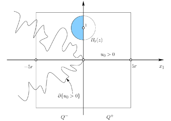
Figure 1. In the coloured half of $B_{r}(z)$ either $u_{0}<0$ or $u_{0}\equiv 0$.

There are three possibilities:

• $u_{0}$ vanishes only on $B_{r}(z)\cap\{x_{1}=0\}$ and $u_{0}>0$ in $B_{r}(z)\cap\{x_{1}<0\}$,

• $u_{0}$ vanishes only on $B_{r}(z)\cap\{x_{1}=0\}$ and $u_{0}<0$ in $B_{r}(z)\cap\{x_{1}<0\}$,

• $u_{0}$ vanishes in $B_{r}(z)\cap\{x_{1}\leq 0\}$.

Notice that Case 1) cannot occur, because it would imply that we deal with a one-phase problem in $B_{r}(z)$ and the $\mathcal{H}^{N}-$density estimate for the zero set would be violated (see Theorem 4.4 in [11]).

Consider now Case 2), and observe that on the hyperplane $\{x_{1}=0\}$ the free boundary condition is satisfied in classical sense:

$$|\nabla u_{0}^{-}|^{p}=\alpha^{p}-\Lambda_{0}=:\gamma^{p}$$

in $B_{r}(z)$. In particular,

(4.8) $$|\nabla u_{0}^{-}|=\gamma>0\quad{\mbox{ on }}\{x_{1}=0\}\cap B_{r}(z).$$

Define

$$\tilde{u}_{0}:=\left\{\begin{array}[]{ll}u^{-}_{0}&{\mbox{ in }}B_{r}(z)\cap\{x_{1}<0\},\\ \gamma x_{1}&{\mbox{ in }}B_{r}(z)\cap\{x_{1}>0\}.\end{array}\right.$$

We claim that

(4.9) $$\Delta_{p}\tilde{u}=0\quad{\mbox{ in }}B_{r/2}(z).$$

Indeed, $\tilde{u}$ is $p$-harmonic in $B_{r}(z)\cap\{x_{1}>0\}$. Moreover, (4.8) yields that $u_{0}^{-}\in C^{2}(\overline{B_{r/2}(z)\cap\{x_{1}<0\}})$, therefore we have that $\Delta_{p}\tilde{u}=0$ pointwise in $\overline{B_{r/2}(z)\cap\{x_{1}<0\}}$, and so (4.9) follows.

Hence, from (4.8), (4.9) and the Unique Continuation Theorem [19] we obtain that $u_{0}^{-}$ must be a linear function in $B_{r/2}(z)\cap\{x_{1}<0\}$. Then, Proposition 5.1 in [19] implies that $u^{-}_{0}$ is a linear function in $\{x_{1}<0\}$. Thus the free boundary condition is satisfied in the classical sense on the plane $\{x_{1}=0\}$ including the origin, and this proves equality in (4.7) in Case 2).

Now we deal with Case 3). We consider a cube $Q=(-5r,5r)\times(-5r,5r)$ centered at the origin such that $B_{r}(z)\subset Q$, and we set $Q^{-}:=Q\cap\{x_{1}<0\}$. Notice that

(4.10) $$u_{0}\leq 0\quad{\mbox{ in }}Q^{-}.$$

In particular, $u_{0}\leq 0$ on $\partial Q^{-}$. According to the remark in Subsection 3.4, $u_{0}$ is a minimizer in $Q^{-}$ of the functional

$$\tilde{J}(u)=\int_{Q^{-}}|\nabla u|^{p}+\Lambda\chi_{\{u>0\}}=\int_{Q^{-}}|\nabla u|^{p}.$$

Therefore $u_{0}$ is $p$-harmonic in $Q^{-}$. By maximum principle, $u_{0}$ cannot achieve its maximum inside $Q^{-}$. This and (4.10) imply that $u_{0}<0$ in $Q^{-}$, and so the free boundary coincides with $\{x_{1}=0\}$.

This concludes the proof of ii)-a) in Definition 4.1. Similarly, one can also prove ii)-b). Hence, $u$ is a viscosity solution, and the desired result follows. ∎

5. On ${\varepsilon}-$monotonicity of $u$ and slab flatness of $\partial\{{u>0}\}$

One of the main free boundary regularity theorems for viscosity solutions is formulated in terms of the ${\varepsilon}-$monotonicity of $u$. More precisely, we have:

Definition 5.1.

We say that $u$ is $\varepsilon-$monotone if there are a unit vector $e$ and an angle $\theta_{0}$ with $\theta_{0}>\frac{\pi}{4}$ (say) and $\varepsilon>0$ (small) such that, for every $\varepsilon^{\prime}\geq\varepsilon$,

(5.1) $$\sup_{B_{\varepsilon^{\prime}\sin\theta_{0}}(x)}u(y-\varepsilon^{\prime}e)\leq u(x).$$

We denote by $\Gamma(\theta_{0},e)$ the cone with axis $e$ and opening $\theta_{0}$.

Definition 5.2.

We say that $u$ is $\varepsilon-$monotone in the cone $\Gamma(\theta_{0},{\varepsilon})$ if it is $\varepsilon-$monotone in any direction $\tau\in\Gamma(\theta_{0},\varepsilon)$.

One can interpret the ${\varepsilon}-$monotonicity of $u$ as closeness of the free boundary to a Lipschitz graph with Lipschitz constant sufficiently close to $1$ if we leave the free boundary in directions $e$ at distance ${\varepsilon}$ and higher. The exact value of the Lipschitz constant is given by $\left(\tan\frac{\theta_{0}}{2}\right)^{-1}$. Then the ellipticity propagates to the free boundary via Harnack’s inequality giving that $\Gamma$ is Lipschitz. Furthermore, Lipschitz free boundaries are, in fact, $C^{1,\alpha}$ regular.

For $p=2$ this theory was founded by L. Caffarelli, see [6, 7, 8]. Recently J. Lewis and K. Nyström proved that this theory is valid for all $p>1$, see [23, 24]. In fact, their argument does not require $u$ to be Lipschitz.

For viscosity solutions we replace the $\varepsilon-$monotonicity with the slab flatness measuring the thickness of $\partial\{{u>0}\}\cap B_{r}(x)$ in terms of the quantity $h(x,r)$ introduced in (2.3). In other words, $h(x,r)$ measures how close the free boundary is to a pair of parallel planes in a ball $B_{r}(x)$ with $x\in\Gamma.$ Clearly, planes are Lipschitz graphs in the direction of the normal, therefore the slab flatness of $\Gamma$ is a particular case of ${\varepsilon}-$monotonicity of $u$.

Hence, under $h_{0}-$flatness of the free boundary we can reformulate the regularity theory “flatness implies $C^{1,\alpha}$” as follows:

Theorem 5.3.

Suppose that $B_{r}(x_{0})\subset\Omega$ with $x_{0}\in\partial\{{u>0}\}$. Then there exists $h>0$ such that if $\Gamma\cap B_{r}(x_{0})\subset\{x\in\mathbb{R}^{N}:-hr<(x-x_{0})\cdot\nu<hr\}$ then $\Gamma\cap B_{r/2}(x_{0})$ is locally $C^{1,\alpha}$ in the direction of $\nu$, for some $\alpha\in(0,1)$.

6. Linear growth vs flatness: Proofs of Theorems A and $\text{A}^{\prime}$

6.1. Dyadic scaling

We first discuss a preliminary result, that we will use for the proof of Theorem A.

Proposition 6.1.

Let $u$ be a local minimizer of $J$ and $x_{0}\in\Gamma\cap B_{1}\subset\Omega$. For any $k\in\mathbb{N}$, set

$$S(k,u):=\sup_{B_{2^{-k}}^{+}(x_{0})}|u|.$$

If $h_{0}>0$ is fixed and $h\left(x_{0},\frac{1}{2^{k}}\right)\geq\frac{h_{0}}{2^{k+1}}$ for some $k$, then

(6.1) $$S(k+1,u)\leq\max\left\{\frac{L2^{-k}}{2},\frac{S(k,u)}{2},\dots,\frac{S(k-m,u)}{2^{m+1}},\dots,\frac{S(0,u)}{2^{k+1}}\right\},$$

for some positive constant $L$, that is independent of $x_{0}$ and $k$.

Otherwise if $h\left(x_{0},\frac{1}{2^{k}}\right)<\frac{h_{0}}{2^{k+1}}$ for some $k$, then $\Gamma\cap B_{2^{-(k+1)}}$ is a $C^{1,\alpha}$ smooth surface, for some $\alpha\in(0,1)$.

Proof.

We first deal with the case $h\left(x_{0},\frac{1}{2^{k}}\right)\geq\frac{h_{0}}{2^{k+1}}$. In order to prove (6.1), we use a contradiction argument discussed in [22]. Hence, we suppose that (6.1) fails, that is there exist integers $k_{j},j=1,2,\ldots$, local minimizers $u_{j}$ and points $x_{j}\in\Gamma_{j}\cap B_{1}$ such that

(6.2) $$h\left(x_{j},\frac{1}{2^{k_{j}}}\right)\geq\frac{h_{0}}{2^{k_{j}+1}}$$

and

(6.3) $$S(k_{j}+1,u_{j})>\max\left\{\frac{j2^{-k_{j}}}{2},\frac{S(k_{j},u_{j})}{2},\dots,\frac{S(k_{j}-m,u_{j})}{2^{m+1}},\dots,\frac{S(0,u_{j})}{2^{k_{j}+1}}\right\}.$$

Since $u_{j}$ is a local minimizer of $J$ in $B_{1}$ and $u_{j}(x_{j})=0$, then $u_{j}$ is bounded (see Theorem 1 in [22]). Namely, there exists a positive constant $M$, that is independent of $j$, such that $S(k_{j}+1,u_{j})\leq M$. Therefore, from (6.3) we have that $M\geq j2^{-k_{j}}/2$, which implies that $2^{k_{j}}\geq j/(2M)$. Hence, $k_{j}$ tends to $+\infty$ when $j\to+\infty$.

We set

(6.4) $$\sigma_{j}:=\frac{2^{-k_{j}}}{S(k_{j}+1,u_{j})}.$$

Using (6.3) once more, we see that

(6.5) $$\sigma_{j}<\frac{2}{j}\to 0\ {\mbox{ as }}j\to+\infty.$$

For any $j$, we now define the function

(6.6) $$v_{j}(x):=\frac{u_{j}(x_{j}+2^{-k_{j}}x)}{S(k_{j}+1,u_{j})}.$$

Then, by construction,

(6.7) $$\sup_{B_{1/2}}|v_{j}|=1.$$

Furthermore, from (6.3) we have that

$$1>\max\left\{\frac{j2^{-k_{j}}}{2S(k_{j}+1,u_{j})},\frac{1}{2}\sup_{B_{1}}|v_{j}|,\dots,\frac{1}{2^{m+1}}\sup_{B_{2^{m}}}|v_{j}|,\dots,\frac{1}{2^{k_{j}+1}}\sup_{B_{2^{k_{j}+1}}}|v_{j}|\right\},$$

which in turn implies that

(6.8) $$\sup_{B_{2^{m}}}|v_{j}|\leq 2^{m+1},\quad\text{for any}\ m<2^{k_{j}}.$$

Finally, since $u_{j}(x_{j})=0$, we have that

(6.9) $$v_{j}(0)=0.$$

Notice that $v_{j}$ is a minimizer (according to its own boundary values) of the scaled functional

(6.10) $$\widehat{J}(v):=\int_{B_{R}}|\nabla v|^{p}+\sigma_{j}^{p}\lambda(v),$$

for $0<R<2^{k_{j}}$ and $j$ large. Indeed, from (6.6) and an easy computation, we get

$$\nabla v_{j}(x)=\frac{2^{-k_{j}}}{S(k_{j}+1,u_{j})}\nabla u_{j}(x_{j}+2^{-k_{j}}x).$$

Hence, by the change of variable $y=x_{j}+2^{-k_{j}}x$ and recalling (6.4),

$$\widehat{J}(v_{j}) = \int_{B_{R}}|\nabla v_{j}(x)|^{p}+\sigma_{j}^{p}\lambda(v)\,dx$$

$$= \int_{B_{R}}\frac{2^{-pk_{j}}}{S(k_{j}+1,u_{j})^{p}}|\nabla u_{j}(x_{j}+2^{-k_{j}}x)|^{p}+\sigma_{j}^{p}\lambda(u_{j}(x_{j}+2^{-k_{j}}x))\,dx$$

$$= \sigma_{j}^{p}\,2^{nk_{j}}\int_{B_{R2^{-k_{j}}}(x_{j})}|\nabla u_{j}(y)|^{p}+\lambda(u_{j})\,dy.$$

Since $u_{j}$ is a minimizer for $J$, the last formula implies that $v_{j}$ is a minimizer for $\widehat{J}$. Hence, from Lemma 3.1 we obtain that for any $q>1$ and $0<R<2^{k_{j}}$ there exists a constant $C=C(R,q)>0$ independent of $j$ such that

$$\max\{\|v_{j}\|_{C^{\alpha}(B_{R})},\|\nabla v_{j}\|_{L^{q}(B_{R})}\}\leq C,$$

for some $\alpha\in(0,1)$. Therefore, by a standard compactness argument, we have that, up to a subsequence,

(6.11) $$v_{j} v j\to+\infty W^{1,q}(B_{R})\cap C^{\alpha}(B_{R}) R$$ converges to some function  as  in  for any fixed .

From (6.7), (6.8) and (6.9) we obtain that

$$\sup_{B_{1/2}}|v|=1,\quad\sup_{B_{2^{m}}}|v|\leq 2^{m+1}\quad{\mbox{and }}\quad v(0)=0.$$

We claim that

(6.12) $$v \mathcal{J}(v):=\int_{B_{R}}|\nabla v|^{p}$$ is a minimizer for the functional .

For this, notice that for any $\varphi\in C^{\infty}_{0}(B_{R})$

(6.13) $$\int_{B_{R}}|\nabla v_{j}|^{p}+\sigma_{j}^{p}\lambda(v_{j})\leq\int_{B_{R}}|\nabla(v_{j}+\varphi)|^{p}+\sigma_{j}^{p}\lambda(v_{j}+\varphi),$$

because  $v_{j}$ is a minimizer for $\widehat{J}$ defined in (6.10). By taking $q>p$ in (6.11), we have that

$$\int_{B_{R}}|\nabla v_{j}|^{p}\to\int_{B_{R}}|\nabla v|^{p}$$

and $$\int_{B_{R}}|\nabla(v_{j}+\varphi)|^{p}\to\int_{B_{R}}|\nabla(v+\varphi)|^{p}$$

as $j\to+\infty$. Moreover, from (6.5) we obtain

$$\int_{B_{R}}\sigma_{j}^{p}\lambda(v_{j})\to 0\quad{\mbox{and }}\quad\int_{B_{R}}\sigma_{j}^{p}\lambda(v_{j}+\varphi)\to 0$$

as $j\to+\infty$. Thus, sending $j\to+\infty$ in (6.13) and using these observations, we get

$$\int_{B_{R}}|\nabla v|^{p}\leq\int_{B_{R}}|\nabla(v+\varphi)|^{p}$$

for any $\varphi\in C^{\infty}_{0}(B_{R})$. This implies (6.12).

Hence, from Liouville’s Theorem (see Theorem 3.3) we deduce that $v$ must be a linear function in $\mathbb{R}^{N}$. Without loss of generality we can take $v(x)=Cx_{1}$ for some positive constant $C$.

On the other hand, (6.2) implies that the following inequality holds true for the function $v_{j}$:

$$h(0,1)\geq\frac{h_{0}}{2}.$$

By the uniform convergence in (6.11), we have that for any $\varepsilon>0$ there is $j_{0}$ such that $|Cx_{1}-v_{j}(x)|<\varepsilon$ whenever $j>j_{0}$. Since $\partial\{{v_{j}>0}\}$ is $h_{0}/2$ thick in $B_{1}$ it follows that there is $y_{j}\in\partial\{{v_{j}>0}\}\cap B_{1}$ such that $y_{j}=e_{1}h_{0}/4+t_{j}e^{\prime}$, for some $t_{j}\in\mathbb{R}$, where $e_{1}$ is the unit direction of $x_{1}$ axis and $e^{\prime}\perp e_{1}$. Then we have that $|C\frac{h_{0}}{4}-0|=|v(y_{j})-v_{j}(y_{j})|<\varepsilon$, which is a contradiction if $\varepsilon$ is small. This finishes the proof of (6.1).

If $h(x_{0},\frac{1}{2^{k}})<\frac{h_{0}}{2^{k+1}}$ for some $k$, we use Theorem 4.2 to obtain that $u$ is also a viscosity solution in the sense of Definition 4.1. Therefore, we can apply the regularity result in Theorem 5.3, thus obtaining the desired claim. This concludes the proof of Proposition 6.1. ∎

6.2. Proof of Theorem A

With the aid of Proposition 6.1 we now complete the proof of Theorem A.

Proof of Theorem A.

The argument in Proposition 6.1 shows that either there are finitely many integers $k$ such that

(6.14) $$h\left(x_{0},\frac{1}{2^{k}}\right)\geq\frac{h_{0}}{2^{k+1}}$$

and

(6.15) $$S(k+1,u)\leq\max\left\{\frac{L2^{-k}}{2},\frac{S(k,u)}{2},\dots,\frac{S(k-m,u)}{2^{m+1}},\dots,\frac{S(0,u)}{2^{k+1}}\right\},$$

or there are infinitely many $k$ such that (6.14) and (6.15) hold true.

In the first case, there exists $k_{0}$ such that $h\left(x_{0},\frac{1}{2^{k_{0}}}\right)<\frac{h_{0}}{2^{k_{0}+1}}$, and so $\Gamma\cap B_{2^{-(k_{0}+1)}}$ is a $C^{1,\alpha}$ smooth surface. In the second case, we have linear growth of $u$ at the free boundary point $x_{0}$ where the flatness does not improve.

Suppose now that we are given $r>0$. Then, either $h(x_{0},r)<\frac{h_{0}}{2}r$ or $h(x_{0},r)\geq\frac{h_{0}}{2}r$. In the first case, we obtain that $\Gamma$ is a $C^{1,\alpha}$-surface. In the second case we argue as follows: there exists $k\in\mathbb{N}$ such that

$$\frac{1}{2^{k+1}}\leq r\leq\frac{1}{2^{k}}.$$

Hence, by the definition of $h$ given in (2.3), we have that

$$h\left(x_{0},\frac{1}{2^{k+1}}\right)\geq h(x_{0},r)\geq\frac{h_{0}}{2}r\geq\frac{h_{0}}{2}\frac{1}{2^{k+1}}.$$

This means that we are in the position to apply Proposition 6.1, that implies linear growth of $u$ at the level $r/2$. ∎

A refinement of Theorem A is given by the following:

Corollary 6.2.

Let $h_{0}$ be the constant given in Theorem A. Then, if $r\in[2^{-k-1},2^{-k})$ and $h(x_{0},r)\geq\frac{h_{0}}{2}r$, we have that

$$\sup_{B_{\frac{r}{2}}(x_{0})}|u|\leq 2Lr,$$

where $L$ is the constant given by Theorem A.

6.3. Alt-Caffarelli-Friedman functional

Here we introduce a functional that is a generalization to any $p>1$ of the one introduced by Alt, Caffarelli and Friedman in the case $p=2$, and we show that this functional is bounded at non-flat free boundary points, thanks to the linear growth ensured by Theorem A.

For this, we let $u=u^{+}-u^{-}$, where $u^{+}:=\max\{0,u\}$ and $u^{-}:=-\min\{0,u\}$. We define the functional

$$\varphi_{p}(r,u,x_{0}):=\frac{1}{r^{4}}\int_{B_{r}(x_{0})}\frac{|\nabla u^{+}|^{p}}{|x-x_{0}|^{N-2}}\,\int_{B_{r}(x_{0})}\frac{|\nabla u^{-}|^{p}}{|x-x_{0}|^{N-2}}$$

where $x_{0}\in\partial\{{u>0}\}$ and $r>0$ is such that $B_{r}(x_{0})\subset\Omega$.

Precisely, we show the following:

Corollary 6.3.

Let $h_{0}$ be fixed, $D\Subset\Omega$ be a subdomain and $x_{0}\in\Gamma\cap D$ be such that $h(r,x_{0})\geq\frac{h_{0}}{2}r$.

Then there exist $M>0,r_{0}>0$ depending only on $N,p,h_{0},\sup_{\Omega}|u|,\Lambda$ and $\operatorname{dist}(D,\partial\Omega)$ such that

$$\varphi_{p}(r,u,x_{0})\leq\frac{M^{2}N^{2}}{4},\quad\forall r\leq r_{0}.$$

Proof.

Since $u^{\pm}$ is nonnegative $p-$subsolution (recall P.1 in Proposition 3.4), we can apply Caccioppoli’s inequality, obtaining that

$$\int_{B_{\rho}(x_{0})}|\nabla u^{\pm}|^{p}\leq\frac{C}{\rho^{p}}\int_{B_{2\rho}(x_{0})}(u^{\pm})^{p}.$$

From this and Corollary 6.2 we have that

$$\int_{B_{\rho}(x_{0})}|\nabla u^{\pm}|^{p}\leq M\rho^{N},$$

for some $M>0$. Hence, using Fubini’s Theorem, we have

$$\int_{B_{r}(x_{0})}\frac{|\nabla u^{\pm}|^{p}}{|x-x_{0}|^{N-2}} = \int_{0}^{r}\frac{1}{\rho^{N-2}}\int_{\partial B_{\rho}(x_{0})}|\nabla u^{\pm}|^{p}$$

$$= \frac{1}{r^{N-2}}\int_{B_{r}(x_{0})}|\nabla u^{\pm}|^{p}+(N-2)\int_{0}^{r}\frac{1}{\rho^{N-1}}\int_{B_{\rho}(x_{0})}|\nabla u^{\pm}|^{p}$$

$$\leq \frac{MN}{2}r^{2},$$

which implies the desired result. ∎

Remark 6.4.

In [15] we prove the converse statement in some sense. More precisely we show that if $N=2$ and $p>2$ is close to $2$ then $\varphi_{p}(r,u,x_{0})$ is discrete monotone.

7. Partial Regularity: Proof of Theorem B

In this section we introduce the set-up in order to prove Theorem B. For this, we recall the notation introduced in Section 2 (recall in particular Definition 2.1 and formula (2.4)). We first show that $\Delta_{p}u^{+}$ is Radon measure.

Lemma 7.1.

Let $u$ be a local minimizer of (1.1). Then, the following statements hold true.

• $\Delta_{p}u^{+}$ is a Radon measure and, for any $x\in\Gamma:=\partial\{{u>0}\}$ and $r>0$ such that $B_{2r}(x)\subset\Omega$, there holds

  (7.1) $$\int_{B_{r}(x)}\Delta_{p}u^{+}\leq\frac{1}{r}\int_{B_{2r}(x)}|\nabla u^{+}|^{p-1}.$$

• For a given subdomain $D\Subset\Omega$ there is $r_{0}>0$ such that

  (7.2) $$\int_{B_{r}(x)}\Delta_{p}u^{+}\geq Cr^{N-1},\quad{\mbox{ for any }}r<r_{0},$$

  for all $x\in\mathscr{N}\cap D$, where $C>0$ depends on $\Lambda$, $N$, $p$, $\operatorname{dist}(D,\partial\Omega)$ and $L$ (given by Theorem A).

• For each $x\in\mathscr{F}$ there is $r(x)>0$ such that

  (7.3) $$\int_{B_{r}(x)}\Delta_{p}u^{+}\geq Cr^{N-1},\quad{\mbox{ for any }}r<r(x),{\mbox{ with }}B_{r(x)}(x)\subset\Omega,$$

  for some $C>0$ that depends on $\Lambda$, $N$, $p$, $\operatorname{dist}(D,\partial\Omega)$ and $x$.

Proof.

We first show (7.1). For this, we take for simplicity $x=0$. Observe that by P.1 in Proposition 3.4 we have that $\Delta_{p}u^{+}\geq 0$ in the sense of distributions. Also, for any $\rho\in(r,2r)$,

$$\int_{B_{\rho}}\Delta_{p}u^{+}=\int_{\partial B_{\rho}}|\nabla u^{+}|^{p-2}\partial_{\nu}u^{+}.$$

Therefore, integrating both sides of the last identity over the interval $(r,2r)$ with respect to $\rho$, we infer that

$$r\int_{B_{r}}\Delta_{p}u^{+} \leq \int_{r}^{2r}\int_{B_{\rho}}\Delta_{p}u^{+}=\int_{r}^{2r}\int_{\partial B_{\rho}}|\nabla u^{+}|^{p-2}\partial_{\nu}u^{+}$$

$$= \int_{B_{2r\setminus B_{r}}}|\nabla u^{+}|^{p-2}\nabla u^{+}\cdot\frac{x}{|x|}$$

$$\leq \int_{B_{2r}}|\nabla u^{+}|^{p-1}.$$

This proves (7.1).

To prove (7.2) we argue towards a contradiction. So, for any $j=1,2,\ldots$, we let $x_{j}\in\mathscr{N}$ and $r_{j}>0$ such that

(7.4) $$\int_{B_{r_{j}}(x_{j})}\Delta_{p}u^{+}<\frac{r_{j}^{N-1}}{j}.$$

We also introduce $v_{j}(x):=\frac{u(x_{j}+r_{j}x)}{r_{j}}$.

Since $x_{j}\in\mathscr{N}$, it follows from Theorem A that $u$ has uniform linear growth at $x_{j}$. This property translates to the scalings of $v$ at $x_{j}$ giving uniform linear growth for the functions $v_{j}$ at the origin, i.e. $|v_{j}(x)|\leq L|x|$ where $L$ is the constant in Theorem A.

Notice that $v_{j}$ is a minimizer of (1.1), so it is locally $C^{\alpha}$, for some $\alpha\in(0,1)$, thanks to Lemma 3.1. Hence $\{v_{j}\}$ is uniformly bounded in $C^{1,\alpha}$, and so is $\|\nabla v_{j}\|_{L^{p}(B_{M})}$ for any fixed $M>0$, thanks to Caccioppoli’s inequality. Therefore, we can extract a subsequence $\{r_{j(m)}\}$ such that $v_{j(m)}\to v_{0}$ as $m\to+\infty$ and $v_{0}$ is a minimizer of $J$ in $B_{2}$. Moreover, by (7.4),

$$\int_{B_{1}}\Delta_{p}v_{0}^{+}=0,$$

with $v_{0}^{+}(0)=0$. As a consequence, $v_{0}^{+}$ vanishes identically in $B_{1}$, by the minimum principle for the $p-$harmonic functions. On the other hand, from Corollary 3.6 we have that $\sup_{B_{\frac{1}{2}}}v_{0}^{+}\geq\frac{c}{2}$, and this gives a contradiction. Thus the proof of (7.2) is finished as well.

The proof of the non-uniform estimate (7.3) follows from a similar argument, by replacing $L$ with a constant $C(x)$ depending on ${\nabla}u^{+}(x)$ and ${\nabla}u^{-}(x)$. ∎

As a consequence of Lemma 7.1, we obtain the first part of Theorem B. More precisely:

Corollary 7.2.

Let $R>0$ be such that $B_{R}\subset\Omega$. Then $\mathcal{H}^{N-1}(\partial\{{u>0}\}\cap B_{R})<\infty$.

Proof.

It follows from (7.2) and (7.3) that for each $x\in\Gamma\cap B_{R}$ there is $r(x)>0$ such that

(7.5) $$\int_{B_{r}(x)}\Delta_{p}u^{+}\geq Cr^{N-1},\quad\text{whenever}\quad r<r(x).$$

Thus $\cup_{x\in\Gamma\cap B_{R}}B_{r(x)}(x)$ is a Besicovitch type covering of $\Gamma\cap B_{R}$. Applying Besicovitch’s Covering Lemma, we have that there is a subcovering $\displaystyle\mathcal{F}=\bigcup_{k=1}^{m(N)}\mathcal{G}_{k}$ of balls $B_{i}:=B_{r(x_{i})}(x_{i})$ such that $\sum_{i}\chi_{B_{i}}\leq A$ for some dimensional constant $A>0$ and

$$\Gamma\cap B_{R}\subset\bigcup_{k=1}^{m(N)}\bigcup_{B_{i}\in\mathcal{G}_{k}}B_{i},$$

where the balls $B_{i}$ in each $\mathcal{G}_{k}$ are disjoint and $\mathcal{G}_{k}$ are countable.

Now we take a small number $\delta>0$, and we observe that if $r(x)>\delta$ then (7.5) holds for any $r<\delta$. Hence, without loss of generality, we take $r(x)<\delta$ for any $x\in\Gamma\cap B_{R}$.

Therefore, using (7.5),

$$C\sum_{B_{i}\in\mathcal{F}}r_{i}^{N-1} \leq \sum_{B_{i}\in\mathcal{F}}\int_{B_{i}}\Delta_{p}u^{+}$$

$$= \sum_{k=1}^{m(N)}\sum_{B_{i}\in\mathcal{G}_{k}}\int_{B_{i}}\Delta_{p}u^{+}$$

$$\leq A\,m(N)\int\limits_{B_{8\delta}(\Gamma\cap B_{R})}\Delta_{p}u^{+},$$

where $B_{8\delta}(\Gamma\cap B_{R})$ is the $8\delta$ neighbourhood of $\Gamma\cap B_{R}$. Thus, choosing a finite covering of $B_{8\delta}(\Gamma\cap B_{R})$ with balls $B_{R_{0}}(z_{j})$, with $j=1,\dots,\ell$, such that $B_{2R_{0}}(z_{i})\subset\Omega$ and $B_{8\delta}(\Gamma\cap B_{R})\subset\cup_{j=1}^{\ell}B_{R_{0}}(z_{j})$ and using (7.1), we have that

$$\mathcal{H}^{N-1}_{\delta}(\Gamma\cap B_{R})\leq\frac{A}{C2^{N-1}}\,\frac{1}{R_{0}}\sum_{j=1}^{\ell}\int_{B_{2R_{0}}(z_{j})}|\nabla u^{+}|^{p-1}<+\infty,$$

and letting $\delta\rightarrow 0$ we arrive at the desired result. ∎

We end this section by the following density type estimate to be used in the final stage of the proof of Theorem B.

Lemma 7.3.

For any subdomain $D\Subset\Omega$ there is a positive constant $c\in(0,1)$ depending on $N,p,\Lambda,\sup_{\Omega}|u|$ and $\operatorname{dist}(D,\partial\Omega)$ such that

(7.6) $$\liminf_{r\to 0}\frac{|\{u\leq 0\}\cap B_{r}(x_{0})|}{|B_{r}(x_{0})|}\geq c,\quad{\mbox{ for any }}x_{0}\in D\cap\partial\{{u>0}\}.$$

Proof.

Notice that if $x_{0}\in\mathscr{F}\cap D$ then (7.6) holds true with $c=1/2$. So we focus on the case in which $x_{0}\in\mathscr{N}\cap D$.

We fix $r>0$ such that $B_{r}(x_{0})\subset\Omega$, and we take a function $v_{r}$ that is $p-$harmonic in $B_{r}(x_{0})$ and such that $u=v_{r}$ on $\partial B_{r}(x_{0})$. Then, reasoning as at the beginning of the proof of Lemma 3.1 (in particular, using (3.1), (3.2), (3.3) and (3.4)), we have that there exists a tame constant $\bar{c}>0$ such that

(7.7) $$\begin{split}\bar{c}\int_{B_{r}(x_{0})}|V({\nabla}u)-V({\nabla}v_{r})|^{2}\,\leq&\int_{B_{r}(x_{0})}|{\nabla}u|^{p}-|{\nabla}v|^{p}\\ \,\leq&\int_{B_{r}(x_{0})}\Lambda({\chi_{\{v_{r}>0\}}}-{\chi_{\{u>0\}}})\\ \,\leq&\int_{B_{r}(x_{0})}\Lambda{\chi_{\{u\leq 0\}}}.\end{split}$$

Now we claim that there is a constant $\Theta>0$ independent of $r$ such that

(7.8) $$v_{r}(x_{0})\geq\Theta r\quad\text{and}\quad\int_{B_{r}(x_{0})}|V({\nabla}u)-V({\nabla}v_{r})|^{2}\geq\frac{\Theta}{r^{p}}\int_{B_{r}(x_{0})}|u-v_{r}|^{p}.$$

Notice that by comparison principle it follows that $v_{r}(x_{0})\geq u(x_{0})=0$. We prove the first inequality in (7.8) using a contradiction argument based on compactness, the second one can be proved analogously.

Suppose that, for any $j=1,2,\ldots$, there are $x_{j}\in D\cap\mathscr{N}$ and $r_{j}>0$ with $B_{2r_{j}}(x_{j})\subset\Omega$ such that

(7.9) $$0<v_{j}(x_{j})\leq\frac{r_{j}}{j}.$$

Now, define $\tilde{v}_{j}(x):=\frac{v_{j}(x_{j}+r_{j}x)}{r_{j}}$ and $\tilde{u}_{j}(x)=\frac{u(x_{j}+r_{j}x)}{r_{j}}$, for any $x\in B_{1}$. We recall that (3.17) implies that $\tilde{u}_{j}$ is a minimizer for $J$ in $B_{1}$. So, it follows from P.1 in Proposition 3.4, Caccioppoli’s inequality and Theorem A that

(7.10) $$\int_{B_{1}}|{\nabla}\tilde{u}_{j}^{\pm}|^{p}\leq C(N)\int_{B_{2}}(\tilde{u}_{j}^{\pm})^{p}\leq C(N)\omega_{N}2^{N+2p}L^{p},$$

where $L$ is the constant introduced in Theorem A.

Also, we observe that $\Delta_{p}\tilde{v}_{j}=0$ in $B_{1}$ and that $\tilde{v}_{j}=\tilde{u}_{j}$ on $\partial B_{1}$. In particular, $\int_{B_{1}}|{\nabla}\tilde{v}_{j}|^{p}\leq\int_{B_{1}}|{\nabla}\tilde{u}_{j}|^{p}.$ This and (7.10) imply that $\|\tilde{v}_{j}\|_{W^{1,p}(B_{1})}\leq C(N)L^{p}$, up to renaming $C(N)$ (recall that $\tilde{u}_{j}^{\pm}$ are $p$-subharmonic, thanks to P.1 in Proposition 3.4).

Moreover, from the local regularity theory for $p-$harmonic functions we have that $\tilde{v}_{j}$ are uniformly $C^{1,\alpha}$ in $B_{\frac{1}{2}}$. Consequently, we have that there is a subsequence (still denoted by $\tilde{v}_{j}$) such that $\tilde{v}_{j}\to v_{0}$ weakly in $W^{1,p}(B_{1})$ and uniformly in $B_{\frac{1}{2}}$, as $j\to+\infty$. In particular, by (7.9),

$$v_{0}(0)=\lim_{j\to\infty}\tilde{v}_{j}(0)=0.$$

As for the sequence $\tilde{u}_{j}$, from (3.17) and Lemma 3.1 we infer that there is a subsequence (still denoted by $\tilde{u}_{j}$) such that ${\nabla}\tilde{u}_{j}\to{\nabla}u_{0}$ strongly in $L^{q}(B_{1})$ for any $q>1$ and $\tilde{u}_{j}\to u_{0}$ uniformly in $\overline{B_{1}}$, as $j\to+\infty$. Furthermore, $u_{0}$ is a minimizer of $J$ and from the convergence of traces it follows that $v_{0}=u_{0}$ on $\partial B_{1}$. Also, by Corollary 3.6 we have that $u_{0}\not=0$, and by Proposition 3.4 we have that $u_{0}$ is $p-$subharmonic in $B_{1}$.

Altogether, we have obtained that

$$\Delta_{p}v_{0}\leq\Delta_{p}u_{0}\;{\mbox{ in }}B_{1},\quad v_{0}=u_{0}\;{\mbox{ on }}\partial B_{1}\quad{\mbox{ and }}v_{0}(0)=u_{0}(0)=0.$$

But this is a contradiction to the comparison principle for $p$-harmonic functions.

The second inequality of (7.8) can be proven analogously.

Now we are ready to finish the proof of (7.6). From (7.7) and (7.8) we have

$$\int_{B_{r}(x_{0})}\Lambda{\chi_{\{u\leq 0\}}} \geq \frac{\bar{c}\Theta}{r^{p}}\int_{B_{r}(x_{0})}|u-v_{r}|^{p}$$

$$\geq \frac{\bar{c}\Theta}{r^{p}}\int_{B_{\kappa r}(x_{0})}|u-v_{r}|^{p}$$

for $0<\kappa<1$ to be chosen later. Observe that by standard gradient estimates

$$|{\nabla}v_{r}(y)|\leq\frac{C}{1-\kappa}\frac{\sup_{B_{r}(x_{0})}|v_{r}|}{r}\leq\frac{CL}{1-\kappa},\quad y\in B_{\kappa r}(x_{0}),$$

up to renaming $C>0$, where the last inequality follows from the maximum principle and Theorem A. Therefore, for any $y\in B_{\kappa r}(x_{0})$

$$|v_{r}(y)-u(y)| \geq |v_{r}(0)-u(y)|-|v_{r}(y)-v_{r}(0)|$$

$$\geq v_{r}(0)-|u(y)|-|v_{r}(y)-v_{r}(0)|$$

$$\geq v_{r}(0)-2L\kappa r-\frac{CL}{1-\kappa}\kappa r$$

$$\geq r\left(\Theta-\kappa L\left(2+\frac{C}{1-\kappa}\right)\right)$$

$$\geq r\frac{\Theta}{2}$$

if we choose $\kappa$ small enough. Returning to (7) we finally get that

$$\frac{|\{u\leq 0\}\cap B_{r}(x_{0})|}{|B_{r}(x_{0})|}\geq\frac{\bar{c}\Theta^{p+1}}{2^{p}\Lambda}\kappa^{N}.$$

This finishes the proof of Lemma 7.3. ∎

8. Blow-up sequence of $u$, end of proof of Theorem B

In this section we study the blow-up sequences of a minimizer of (1.1) and prove a simple compactness result, that we use to conclude the proof of Theorem B. For this, let $u$ be a minimizer of $J$ and $x_{0}\in\partial\{{u>0}\}$. Consider a sequence of balls $B_{\rho_{k}}(x_{0})$, with $\rho_{k}\to 0$. We call the sequence of functions defined by

(8.1) $$u_{k}(x)=\frac{u(x_{0}+\rho_{k}x)}{\rho_{k}}$$

the blow-up sequence of $u$ with respect to $B_{\rho_{k}}(x_{0})$. Clearly $u_{k}$ is also a local minimizer.

Proposition 8.1.

Let $x_{0}\in\mathscr{N}$ and $u_{k}$ be a blow-up sequence. Then there is a blow-up limit $u_{0}:\mathbb{R}^{N}\to\mathbb{R}$ with linear growth such that for a subsequence

• $u_{k}\to u_{0}$ in $C_{loc}^{\alpha}(\mathbb{R}^{N})$ for any $\alpha\in(0,1)$,

• ${\nabla}u_{k}\to{\nabla}u_{0}$ weakly in $W^{1,q}$ for any $q>1$,

• $\partial\{{u_{k}>0}\}\to\partial\{{u_{0}>0}\}$ locally in Hausdorff distance,

• ${\chi_{\{u_{k}>0\}}}\to{\chi_{\{u_{0}>0\}}}$ in $L_{loc}^{1}(\mathbb{R}^{N})$.

Proof.

The first and second claims follow from Lemma 3.1 and a customary compactness argument to show that the blow-up limit $u_{0}$ exists.

We recall the definition of Hausdorff distance:

$$d_{\mathcal{H}}(F,G):=\inf\left\{\delta:F\subset\bigcup_{x\in G}B_{\delta}(x),G\subset\bigcup_{x\in F}B_{\delta}(x)\right\}.$$

Let $B_{r}:=B_{r}(z_{0})$ be a ball not intersecting $\partial\{u_{0}>0\}$. If $u_{0}>0$ in $\overline{B_{r}}$ then, by locally uniform convergence, $u_{k}>0$ in $B_{\frac{r}{2}}$, thus implying that $\partial\{u_{k}>0\}\cap B_{r/2}=\emptyset$. As for the case $u_{0}\leq 0$ in $B_{r}$, it follows from Proposition 3.5 that $\frac{1}{r}\fint_{B_{r}}(u^{+}_{0})<{\varepsilon}$, for any small ${\varepsilon}>0$. Thus, by the uniform convergence, we have that $\frac{1}{r}\fint_{B_{r}}(u^{+}_{k})<{\varepsilon}$ if $k$ is sufficiently large. From Proposition 3.5 we conclude that $u_{k}\leq 0$ in $B_{r/2}$. In both cases we infer that $\partial\{{u_{k}>0}\}$ does not intersect $B_{r/2}$ if $k$ is large enough.

Conversely, if $B_{r}$ does not intersect $\partial\{{u_{k}>0}\}$ for any large $k$, then either $u_{k}>0$ in $B_{r}$ or $u_{k}\leq 0$ in $B_{r}$. In the first case, $u_{k}$ is $p-$harmonic in $B_{r}$ and hence so is $u_{0}$. Consequently, either $u_{0}>0$ in $B_{r}$ or $u_{0}\equiv 0$ in $B_{r}$. Thus $B_{r}$ does not intersect $\partial\{{u_{0}>0}\}$. In the second case, we have that $u_{0}\leq 0$, so that again $\partial\{{u_{0}>0}\}$ does not intersect $B_{r}$.

Reasoning as above and using a covering argument one can show that, for a fixed compact set $D$, the quantity $\delta$ in the definition of $d_{\mathcal{H}}$, with $G=\partial\{u_{0}>0\}\cap D$ and $F=\partial\{u_{k}>0\}\cap D$, can be chosen as small as we wish.

The last statement follows from the non-degeneracy of $u^{+}$ given by Corollary 3.6, the convergence of $\partial\{{u_{k}>0}\}\to\partial\{{u_{0}>0}\}$ in Hausdorff distance and the fact that the $N$-dimensional Hausdorff measure $\mathcal{H}^{N}(\partial\{{u_{0}>0}\})=0$, since $u_{0}$ is also minimizer and Corollary 7.2 applies. Hence the proof of Proposition 8.1 is concluded. ∎

Remark 8.2.

In view of Proposition 3.5 we see that when we consider the blow-up of a minimizer, the limit cannot vanish, no matter how many times we blow-up the minimizer $u$ at a non-flat point.

We now finish the proof of Theorem B. More precisely, we show that

(8.2) $$\mathcal{H}^{N-1}\left((\partial\{{u>0}\}\setminus\partial_{\text{red}}\{{u>0}\})\cap B_{R}\right)=0.$$

First observe that $\mathscr{N}\subset\partial\{u>0\}\setminus\partial_{\rm red}\{u>0\}$, see the discussion in Section 5. Since the current boundary $T:=\partial(\mathbb{R}^{N}\rule[-1.42262pt]{0.5pt}{11.38109pt}\rule[-1.42262pt]{11.38109pt}{0.5pt}\{u>0\}\cap B_{R}(0))$ is representable by integration, $\|T\|=\int_{B_{R}(0)}|D{\chi_{\{u>0\}}}|$, we get from Section 4.5.6. on page 478 of [17] that

(8.3) $$\begin{split}&{\mbox{$\partial\{u>0\}\setminus\partial_{\rm red}\{u>0\}=K_{0}\cup K_{+}$, where $\mathcal{H}^{N-1}(K_{+})=0$}}\\ &{\mbox{and for $x_{1}\in K_{0}$, $r^{1-N}\mathcal{H}^{N-1}(\partial_{\rm red}\{u>0\}\cap B_{r}(x_{1}))\rightarrow 0$ as $r\rightarrow 0$.}}\end{split}$$

Let us show that

(8.4) $$K_{0}=\emptyset.$$

To see this, for $k\in\mathbb{N}$, we define $u_{k}(x):=\frac{u(x_{1}+r_{k}x)}{r_{k}}$, where $r_{k}\to 0$ as $k\to+\infty$. By the compactness properties obtained in Proposition 8.1, we have that $u_{k}\rightarrow u_{0}$, as $k\to+\infty$, for some function $u_{0}$ and, for any test function $\varphi$,

$$\int_{B_{R}}{\chi_{\{u_{0}>0\}}}\operatorname{div}\varphi\longleftarrow\int_{B_{R}}{\chi_{\{u_{k}>0\}}}\operatorname{div}\varphi=r^{1-N}_{k}\int_{B_{Rr_{k}}(x_{1})}{\chi_{\{u>0\}}}\operatorname{div}\varphi\left(\frac{x-x_{1}}{r_{k}}\right)$$

$$\leq\sup\varphi\,r_{k}^{1-N}\mathcal{H}^{N-1}(\partial_{\rm red}\{u>0\}\cap B_{Rr_{k}}(x_{1}))\longrightarrow 0\qquad{\rm{as}}\qquad k\rightarrow+\infty,$$

where (LABEL:rew21) was also used.

Hence we infer that ${\chi_{\{u_{0}>0\}}}$ is a function of bounded variation which is constant a.e. in $B_{R}$. The positive Lebesgue density property of $\{u\leq 0\}$ obtained in Lemma 7.3 and translated to $u_{0}$ through compactness, and the strong maximum principle for $p-$harmonic functions demand $u_{0}$ to be zero. This is in contradiction with the non-degeneracy of $u^{+}$ stated by Proposition 3.5 (notice that, by a compactness argument, the non-degeneracy property translates to $u_{0}$). Thus (8.4) is proved.

From (LABEL:rew21) and (8.4) we obtain that $\mathcal{H}^{N-1}\left((\partial\{u>0\}\setminus\partial_{\rm red}\{u>0\})\cap B_{R}\right)=0$. The proof of Theorem B is then finished.

9. Proof of Theorem C

With the aid of Theorem A, in this section we complete the proof of Theorem C.

Proof of Theorem C.

It is well-know that in order to prove the estimate (2.5) it is enough to show that $u$ grows linearly away from the free boundary. For this, let $0\in\partial\{{u>0}\}$ and $B_{\frac{1}{4}}\Subset\Omega$. Notice that, if for all $k\in\mathbb{N}$, $k\geq 2$, we have that $h(0,2^{-i})\geq h_{0}2^{-i-1}$, then it follows from Theorem A that $\sup_{B_{r}}|u|\leq 2Lr$. Therefore, suppose that there is $k_{0}\in\mathbb{N}$ such that

(9.1) $$h\left(0,\frac{1}{2^{j}}\right)\geq\frac{h_{0}}{2}\frac{1}{2^{j}},\quad j=2,\dots,k_{0}-1,$$

but

(9.2) $$h\left(0,\frac{1}{2^{k_{0}}}\right)<\frac{h_{0}}{2}\frac{1}{2^{k_{0}}}.$$

From (9.1) and Proposition 6.1 (or Corollary 6.2) it follows that

(9.3) $$\sup_{B_{\frac{1}{2^{k_{0}-1}}}}|u|=\sup_{B_{\frac{1}{2}\frac{1}{2^{k_{0}-2}}}}|u|\leq 2L\frac{1}{2^{k_{0}-2}}=\frac{4L}{2^{k_{0}-1}}.$$

Denote $R_{0}:=\frac{1}{2^{k_{0}-1}}$ and introduce

(9.4) $$v_{0}(x):=\frac{u(R_{0}x)}{R_{0}},\quad x\in B_{1},$$

then by (3.17) it follows that $v_{0}$ is a minimizer in $B_{1}$. Furthermore, (9.3) yields

(9.5) $$\sup_{B_{1}}|v_{0}|\leq 4L$$

and by (9.2) we see that $\partial\{{v_{0}>0}\}\cap B_{\frac{1}{2}}$ is $h_{0}/2$ flat. Therefore, we infer from the second part of Theorem A that there are $\delta\in(0,\frac{1}{2})$ and $\alpha>0$ depending on $N$, $p$, $\Lambda$, $h_{0}$ and $4L$ such that $\partial\{{v_{0}>0}\}\cap B_{\delta}$ is $C^{1,\alpha}$ regular. Applying the boundary gradient estimates for $p-$harmonic functions we finally obtain

(9.6) $$\sup_{B_{\frac{\delta}{2}}}|{\nabla}v_{0}^{\pm}(x)|\leq 4LC_{0}$$

for some tame constant $C_{0}>0$. Recalling (9.4) and (9.3) we conclude that

$$\sup_{B_{r}}|u|\leq\frac{16L}{\delta}r,\quad\forall r<r_{0}$$

for some small universal constant $r_{0}$. This completes the proof of Theorem C. ∎

Appendix A Viscosity solutions and linear development

Here we show Lemma 4.3.

Proof of Lemma 4.3.

We first show a). Without loss of generality, we may assume that $x_{0}=0$ and $\nu=e_{N}$. Let $B:=B_{R}(y_{0})$ be a touching ball at $0\in\Gamma$, for some $y_{0}\in\Omega$ and $R>0$.

Now, we want to establish (4.4). For this, we first construct a function that can be used as a barrier to control $u$ from below in the ring $B_{R}(y_{0})\setminus B_{R/2}(y_{0})$. We consider the scaled $p-$capacitary function $H$, that is $p$-harmonic in $B_{R}(y_{0})\setminus B_{R/2}(y_{0})$, that vanishes on $\partial B_{R}(y_{0})$ and that is equal to 1 on $\partial B_{R/2}(y_{0})$. Observe that near the origin

(A.1) $$H(x)=c(N,R)\,x_{N}+o(|x|),$$

for some $c(N,R)>0$.

Using the Harnack inequality we see that $u(x)\geq c_{0}u(y_{0})$ in $\bar{B}_{R/2}(y_{0})$, for some $c_{0}>0$. Thus, multiplying $H$ with a suitable constant $\sigma:=c_{0}u(y_{0})$ we obtain that $\sigma H\leq u$ on $\partial B_{R/2}(y_{0})$. Moreover, $u\geq 0=\sigma H$ on $\partial B_{R}(y_{0})$. Hence, by comparison principle, we get that

$$u(x)\geq\sigma H(x)\quad{\mbox{ in }}B_{R}(y_{0})\setminus B_{R/2}(y_{0}).$$

From this and (A.1) we obtain that

(A.2) $$u(x)\geq\sigma c(N,R)x_{N}+o(|x|)$$

near the origin.

Now we take $k_{0}$ the smallest positive integer such that $2^{-k_{0}}\leq R/2$ and we define

(A.3) $$A_{k}:=\sup\{m:u(x)\geq mx_{N}{\mbox{ in }}B_{2^{-(k_{0}+k)}}\cap B_{R}(y_{0})\},\qquad k=0,1,2,\dots.$$

Thanks to (A.2) the set of numbers $m$ in the definition of $A_{k}$ is not empty. Notice also that the sequence $\{A_{k}\}$ is increasing, and so we let $A:=\sup A_{k}$.

We observe that

(A.4) $$A>0.$$

Indeed, since $u(x)\geq\sigma H(x)$ in $\overline{B_{R}(y_{0})\setminus B_{R/2}(y_{0})}$ then $A_{0}>0$. This implies (A.4), because  $A_{k}$ is increasing.

If $A=\infty$, then $u$ grows faster than any linear function at $0$. While, if $A<\infty$, then (4.4) holds true.

Now we claim that equality in (4.4) holds in any non-tangential domain. In what follows we denote by

(A.5) $$\mathcal{B}:=B_{s}(e_{N}/2),\ {\mbox{ for some small $s>0$, }}\ \mathcal{D}_{k}:=B_{R/{r_{k}}}(y_{0}/r_{k})\cap B_{1}\ {\mbox{ and }}\ r_{k}:=2^{-(k+k_{0})}.$$

If the claim fails then there exist a sequence of points $x^{k}\in B_{R}(y_{0})$ and $\delta_{0}>0$ such that

(A.6) $$u(x^{k})>Ax_{N}^{k}+\delta_{0}|x^{k}|\quad{\mbox{ and }}\quad|x_{k}|=r_{k}\sim\operatorname{dist}(x^{k},\partial B_{R}(y_{0})).$$

Now let $u_{k}(x):=\frac{u(r_{k}x)}{r_{k}}$. Notice that (A.6) implies that

$$u_{k}(y^{k})>Ay_{N}^{k}+\delta_{0},$$

where $y^{k}:=x^{k}/r_{k}\in\partial B_{1}\cap B_{R/r_{k}}(y_{0}/r_{k})$. This implies that

(A.7) $$u_{k}(x)-Ax_{N}\geq c_{0}\,\delta_{0}$$

on some fixed portion of $\partial B_{1}\cap B_{R/r_{k}}(y_{0}/r_{k})$, for some $c_{0}>0$. So, (A.7) and the Harnack inequality give that

(A.8) $$u_{k}(x)-Ax_{N}\geq\frac{c_{0}\delta_{0}}{100}\quad{\mbox{ in }}\mathcal{B},$$

where $\mathcal{B}$ has been introduced in (A.5) and we can take $s=\frac{1}{8}$.

Since $u_{k}$ are uniformly $C^{1,\alpha}_{loc}$ in $B_{2}\cap B_{R/r_{k}}(y_{0}/r_{k})$ and uniformly continuous in $B_{2}\cap\{x_{N}>0\}$, we have that, up to a subsequence, $u_{k}$ converges uniformly to some $u_{0}\geq 0$ in $B_{1}\cap\{x_{N}\geq 0\}$. Therefore, by construction of $A$,

(A.9) $$u_{0}(x)-Ax_{N}\geq 0\quad{\mbox{ in }}\partial B_{1}\cap\{x_{N}\geq 0\}.$$

We recall (A.5) and define functions $w_{k}$ as solutions to the following boundary value problem

(A.10) $$\left\{\begin{array}[]{lll}\Delta_{p}w_{k}=0&\ {\mbox{ in }}\mathcal{D}_{k}\setminus\mathcal{B},\\ w_{k}=A_{k}x_{N}+\frac{c_{0}\delta_{0}}{200}&\ {\mbox{ on }}\partial\mathcal{B},\\ w_{k}=A_{k}x_{N}&\ {\mbox{ on }}\partial\mathcal{D}_{k}.\end{array}\right.$$

Now from the definition of $A_{k}$ in (A.3) we have that $u_{k}(x)\geq A_{k}x_{N}$ in $B_{R/r_{k}}(y_{0}/r_{k})\cap B_{1}=\mathcal{D}_{k}$, and so $w_{k}=A_{k}x_{N}\leq u_{k}$ on $\partial\mathcal{D}_{k}$. Moreover, on $\partial\mathcal{B}$ we have that $w_{k}=A_{k}x_{N}+\frac{c_{0}\delta_{0}}{200}\leq Ax_{N}+\frac{c_{0}\delta_{0}}{200}\leq u_{k}$, thanks to (A.8). By comparison principle we get that $w_{k}\leq u_{k}$ in $\mathcal{D}_{k}\setminus\mathcal{B}$.

By construction $w_{k}\to w_{0}$ uniformly in $B_{\mu}\cap\mathcal{D}_{k}$ and

(A.11) $$\|w_{k}-w_{0}\|_{L^{\infty}(\mathcal{D}_{k})}\leq\varepsilon_{k}\to 0.$$

From the stability of $C^{1,\alpha}$ norm in $B_{3/16}^{+}$ (recall that we chose $s=1/8$ in (A.5)) we conclude

(A.12) $$\|\nabla(w_{k}-w_{0})\|_{C^{\alpha}(B_{3/16}^{+}\cap\mathcal{D}_{k})}\leq\varepsilon_{k}.$$

This allows to estimate the Hölder norm of $\nabla(w_{k}-w_{0})$ near the flat portion of the boundary of $B^{+}_{3/16}$.

By Hopf’s Lemma there is $\gamma>0$ such that $w_{0}\geq(A+\gamma)x_{N}+o(|x|)$ near the origin. Combining we get that

$$u_{k} \geq w_{k}=w_{k}-w_{0}+w_{0}\geq w_{k}-w_{0}+(A+\gamma)x_{N}+o(|x|)$$

$$\geq (A+\gamma)x_{2}+o(|x|)-\varepsilon_{k}x_{N}$$

$$\geq (A+\frac{\gamma}{2})x_{N}+o(|x|)$$

$$\geq (A+\frac{\gamma}{4})x_{N}$$

in $B_{1/2}^{+}\cap B_{R/r_{k}}(y_{0}/r_{0})$. Returning to $u$ we get that

$$u(x)\geq(A+\frac{\gamma}{4})x_{N}\geq(A_{k+1}+\frac{\gamma}{8})x_{N}$$

in $B_{r_{k}/2}\cap B_{R}(y_{0})=B_{r_{k+1}}\cap B_{R}(y_{0})$. This is a contradiction with the definition of $A_{k}$ in (A.3).

Hence, (4.4) holds true in any non-tangential domain, and this concludes the proof of part a).

Now we show part b). For this, we take a ball $B_{R}(y_{0})$ touching $x_{0}$ from outside $\Omega$. We construct the barrier as follows: we let $\eta$ to be a $p$-harmonic function in $B_{2R}(y_{0})\setminus B_{R}(y_{0})$, such that $\eta=0$ on $\partial B_{R}(y_{0})$ and $\eta=\max_{\partial B_{2R}(y_{0})}u$ on $\partial B_{2R}(y_{0})$. Then, from comparison principle we have that $u\leq\eta$ in $B_{2R}(y_{0})\cap\Omega$. Moreover, by Hopf’s Lemma

(A.14) $$\eta(x)=C(N,R)x_{N}+o(|x|)$$

near the origin, for some $C(N,R)>0$.

We take $k_{0}$ to be the smallest positive integer such that $2^{-k_{0}}<R/2$, and we define

$$\beta_{0}:=\inf\{m:m\eta(x)\geq u(x){\mbox{ in }}B_{2^{-k_{0}}}\cap B_{R}^{c}(y_{0})\},$$

and, for any $k\geq 1$,

$$\beta_{k}:=\inf\{m:m\eta(x)\geq u(x){\mbox{ in }}B_{2^{-(k_{0}+k)}}\cap B_{R}^{c}(y_{0})\}.$$

Since $\beta_{k}$ is a decreasing sequence, we can take $\tilde{\beta}:=\inf\beta_{k}$. Hence, $\tilde{\beta}\geq 0$, and, setting $\beta:=\tilde{\beta}C(N,R)$, from (A.14) we deduce (4.5).

In order to prove equality in (4.5) in every non-tangential domain, one can proceed as in the proof of part a). This concludes the proof of Lemma 4.3. ∎

References

- [1] H.W. Alt, L.A. Caffarelli, A. Friedman: Variational problems with two phases and their free boundaries. Trans. Amer. Math. Soc. 282 (1984), no. 2, 431–461.
- [2] H.W. Alt, L.A. Caffarelli, A. Friedman; A free boundary problem for quasilinear elliptic equations. Ann. Scuola Norm. Sup. Pisa Cl. Sci. (4) 11 (1984), no. 1, 1–44.
- [3] G. Astarita, G. Marrucci: Principles of non-Newtonian fluid mechanics. MacGraw Hill, London, New York, 1974.
- [4] G. Birkhoff, E.H. Zarantonello: Jets, Wakes, and Cavities. Academic Press, 1957.
- [5] J.E. Braga, D.R. Moreira: Uniform Lipschitz regularity for classes of minimizers in two phase free boundary problems in Orlicz spaces with small density on the negative phase. Ann. Inst. H. Poincaré Anal. Non Linéaire 31 (2014), no. 4, 823–850.
- [6] L.A. Caffarelli: A Harnack inequality approach to the regularity of free boundaries. I. Lipschitz free boundaries are . Rev. Mat. Iberoamericana 3 (1987), no. 2, 139–162.
- [7] L.A. Caffarelli: A Harnack inequality approach to the regularity of free boundaries. III. Existence theory, compactness, and dependence on . Ann. Scuola Norm. Sup. Pisa Cl. Sci. (4) 15 (1988), no. 4, 583–602.
- [8] L.A. Caffarelli: A Harnack inequality approach to the regularity of free boundaries. II. Flat free boundaries are Lipschitz. Comm. Pure Appl. Math. 42 (1989), no. 1, 55–78.
- [9] L.A. Caffarelli, S. Salsa: A geometric approach to free boundary problems. Graduate Studies in Mathematics, 68. American Mathematical Society, Providence, RI, 2005. x+270 pp.
- [10] A. Cianchi: Continuity properties of functions from Orlicz-Sobolev spaces and embedding theorems. Ann. Scuola Norm. Sup. Pisa Cl. Sci. (4) 23 (1996), no. 3, 575–608.
- [11] D. Danielli, A. Petrosyan: A minimum problem with free boundary for a degenerate quasilinear operator. Calc. Var. Partial Differential Equations 23 (2005), no. 1, 97–124.
- [12] D. Danielli, A. Petrosyan, H. Shahgholian: A singular perturbation problem for the -Laplace operator. Indiana Univ. Math. J. 52 (2003), no. 2, 457–476.
- [13] E. DiBenedetto, J. Manfredi, On the higher integrability of the gradient of weak solutions of certain degenerate elliptic systems. Amer. J. Math. 115 (1993), no. 5, 1107–1134.
- [14] L. Diening, B. Stroffolini, A. Verde: Everywhere regularity of functionals with -growth. Manuscripta Math. 129 (2009), no. 4, 449–481.
- [15] S. Dipierro, A.L. Karakhanyan: A new discrete monotonicity formula with application to a two-phase free boundary problem in dimension 2. Preprint, http://arxiv.org/abs/1509.00277
- [16] F. Duzaar, G. Mingione: The -harmonic approximation and the regularity of -harmonic maps. Calc. Var. Partial Differential Equations 20 (2004), no. 3, 235–256.
- [17] H. Federer; Geometric measue theory. Springer-Verlag, Berlin, Heidelberg and New York, 1969.
- [18] M. Giaquinta: Multiple integrals in calculus of variations and nonlinear elliptic systems. Annals of Mathematics Studies, 105. Princeton University Press, Princeton, NJ, 1983. vii+297 pp.
- [19] S. Granlund, N. Marola: On the problem of unique continuation for the -Laplace equation. Nonlinear Anal. 101 (2014), 89–97.
- [20] M.I. Gurevich: The theory of jets in an ideal fluid. Translated from the Russian by R. E. Hunt. Translation edited by E. E. Jones and G. Power. International Series of Monographs in Pure and Applied Mathematics, Vol. 93 Pergamon Press, Oxford-New York-Toronto, Ont. 1966 viii+412 pp.
- [21] A.L. Karakhanyan: Up-to boundary regularity for a singular perturbation problem of -Laplacian type. J. Differential Equations 226 (2006), no. 2, 558–571.
- [22] A.L. Karakhanyan: On the Lipschitz regularity of solutions of minimum problem with free boundary. Interfaces Free Bound. 10 (2008), no. 1, 79–86.
- [23] J.L. Lewis, K. Nyström: Regularity of Lipschitz free boundaries in two-phase problems for the -Laplace operator. Adv. Math. 225 (2010), 2565–2597.
- [24] J.L. Lewis, K. Nyström: Regularity of flat free boundaries in two-phase problems for the -Laplace operator. Ann. Inst. H. Poincaré Anal. Non Linéaire 29 (2012), 83–108.
- [25] J. Malý, W.P. Ziemer: Fine regularity of solutions of elliptic partial differential equations. Mathematical Surveys and Monographs, 51. American Mathematical Society, Providence, RI, 1997. xiv+291 pp.
- [26] J.R. Philip: -diffusion. Austral. J. Phys. 14 (1961) 1–13.
- [27] P. Tolksdorf: On the Dirichlet problem for quasilinear equations in domains with conical boundary points. Comm. Partial Differential Equations 8 (1983), no. 7, 773–817.