Fast GPU-based calculations in few-body quantum scattering

Abstract

A principally novel approach towards solving the few-particle (many-dimensional) quantum scattering problems is described. The approach is based on a complete discretization of few-particle continuum and usage of massively parallel computations of integral kernels for scattering equations by means of GPU. The discretization for continuous spectrum of a few-particle Hamiltonian is realized with a projection of all scattering operators and wave functions onto the stationary wave-packet basis. Such projection procedure leads to a replacement of singular multidimensional integral equations with linear matrix ones having finite matrix elements. Different aspects of the employment of a multithread GPU computing for fast calculation of the matrix kernel of the equation are studied in detail. As a result, the fully realistic three-body scattering problem above the break-up threshold is solved on an ordinary desktop PC with GPU for a rather small computational time.

1 Introduction

Solution of few-body scattering problems, especially above the three-body breakup threshold, no matter in differential or integral formalism, involves a very large amount of calculations and therefore requires extensive use of modern computational facilities such as powerful supercomputers. As a vivid example, we note that one of the most active and successful groups in the world in this area — the Bochum–Cracow group guided up to recent time by Prof. W. Glöckle (who passed away recently) — employed for such few-nucleon calculations the fastest in Europe supercomputer from JSC in Jülich with the architecture of Blue Gene [1, 2]. Quite recently, new methods for solving Faddeev and Faddeev-Yakubovsky few-body scattering equations using (in one way or another) the bases of square-integrable functions have been developed [3], which allow to simplify significantly the numerical solution schemes. Nevertheless, the treatment of realistic three- and four-body scattering problems includes a tremendous numerical labor and, as a result, still can be done only by a few groups over the world that hinders the development of these important studies.

However, recently there appeared a new possibility to use the Graphics Processing Units (GPU) for such time-consuming calculations. This can transform an ordinary PC into a supercomputer. There is no necessity to argue that such variant is unmeasurably cheaper and more accessible for many researchers in the world. However, due to the special GPU architecture usage of GPU is effective only for those problems where numerical schemes of solution can be realized with a high degree of parallelism. The high effectiveness of the so-called General Purpose Graphics Processing Unit (GPGPU) computing has been demonstrated in many areas of quantum chemistry, molecular dynamics, seismology, etc. (see the detailed description of different GPU applications in refs. [4, 5, 6, 7]). Nevertheless, according to present authors’ knowledge, GPU computing still has not been used widely for a solution of few-body scattering problems (we know only two researches but they are dedicated to the ab initio calculation of bound states [8] and also resonances in the Faddeev-type formalism [9]). Thus, in this paper we would like to study in detail just the effectiveness of GPU computing in solving general few-body scattering problems.

In the case when the colliding particles have inner structures and can be excited in the scattering process, i.e. should be treated as composite ones (e.g., nucleon isobars) the numerical complexity of the problem is increased additionally, so that without a significant improvement of the whole numerical scheme the practical solution of such multichannel problems becomes to be highly nontrivial even for a supercomputer. Thus, the development of new methods in few-body scattering which can be adapted for massively parallel realization is of interest nowadays. We propose here a novel approach in this area which includes two main components:

(i) A complete discretization of the continuous spectrum of the scattering problem, i.e. the replacement of continuous momenta and energies with their discrete counterparts, by projecting all the scattering functions and operators onto a space spanned on the basis of the stationary wave packets [10, 11, 12, 13]. As a result, the integral equations of the scattering theory (like the Lippmann–Schwinger, Faddeev etc. equations) are replaced with their matrix analogs. Moreover, due to an ordinary $L_{2}$ normalization of the stationary wave packets one can solve a scattering problem almost fully similarly to bound-state problems, i.e. without explicit account of the boundary conditions (which are rather nontrivial above few-body breakup thresholds). The main feature of this discretization procedure is that all the constituents in the equations are represented with finite matrices, elements of which are calculated independently. So, this approach is just quite suitable for parallelization and implementation on GPU.

(ii) The numerical solution of the resulting matrix equations with wide usage of the multithread computing on GPU.

In the present paper, we adapt the general wave-packet discretization algorithm for GPU implementation by an example of calculating the elastic scattering amplitude in three-nucleon system with realistic interactions. Also different aspects related to GPU computing are studied and runtimes for CPU and GPU mode calculations are compared.

The paper is organized as follows. In the section II we briefly recall the main features of the wave-packet continuum discretization approach towards solving two- and three-body scattering problems. The numerical scheme for a practical solution of the $nd$ elastic scattering problem in a discretized representation is described in Section III. In the next Section IV we discuss the properties of GPU computing for the above problem and test some illustrative examples while in the Section V the results for the $nd$ elastic scattering with realistic $NN$ interaction are presented. The conclusions are given in the last Section VI.

2 Continuum discretization with stationary wave-packets in few-body scattering problems

In this section we outline briefly the method of stationary wave packets that is necessary for understanding the subsequent material by reader. For detail we refer to our previous original papers [11, 13] and the recent review [10].

2.1 Stationary wave packets for two-body Hamiltonian

Let us introduce some two-body Hamiltonian $h=h_{0}+v$ where $h_{0}$ is a free Hamiltonian (the kinetic energy operator) and $v$ is an interaction. Stationary wave packets (WPs) are constructed as integrals of exact scattering wave functions $|\psi_{p}\rangle$ (non-normalized) over some momentum intervals $\{\Delta_{i}\equiv[p_{i-1},p_{i}]\}_{i=1}^{N}$:

$$|z_{k}\rangle=\frac{1}{\sqrt{C_{k}}}\int_{{\Delta}_{k}}w(p)|\psi_{p}\rangle dp,\quad C_{k}=\int_{\Delta_{k}}|w(p)|^{2}dp.$$ (1)

Here $p=\sqrt{2mE}$ is relative momenta, $m$ is the reduced mass of the system, $w(p)$ is a weight function and $C_{k}$ is the corresponding normalization factor.

The set of WP states (1) has a number of interesting and useful properties [10]. First of all, due to the integration in eq. (1), the WP states have a finite normalization as bound states. The set of WP functions together with the possible bound-state wave functions $|z^{b}_{n}\rangle$ of the Hamiltonian $h$ form an orthonormal set and can be employed as a basis similarly to any other $L_{2}$ basis functions, which are used to project wave functions and operators [10]. (To simplify notations, we will omit below the superscript $b$ for bound-states and will differ them from WP states just by their index $n\leq N_{b}$.)

The matrix of Hamiltonian $h$ is diagonal in such a WP basis. The resolvent $g(E)=[E+{\rm i}0-h]^{-1}$ for Hamiltonian $h$ has also a diagonal representation in the subspace spanned on the WP basis:

$$g(E)\approx\sum_{n=1}^{N_{b}}\frac{|z_{n}\rangle\langle z_{n}|}{E-\epsilon_{n}^{*}}+\sum_{k=N_{b}+1}^{N}|z_{k}\rangle g_{k}(E)\langle z_{k}|,$$ (2)

where $\epsilon_{n}^{*}$ are the bound-state energies and eigenvalues $g_{k}(E)$ can be expressed by explicit formulas [10].

2.2 Free wave-packet basis

Useful particular case of stationary wave packets is free WP states which are defined for the free Hamiltonian $h_{0}$. As in the general case, the continuum of $h_{0}$ (in every spin-angular channel $\alpha$) is divided onto non-overlapping intervals $\{\mathfrak{D}_{i}\equiv[{\cal E}_{i-1},{\cal E}_{i}]\}_{i=1}^{N}$ and two-body free wave-packets are introduced as integrals of exact free-motion wave functions $|p\rangle$ (an index $\alpha$ which marks possible quantum numbers we will omit where is possible):

$$|x_{i}\rangle=\frac{1}{\sqrt{B_{i}}}\int_{\mathfrak{D}_{i}}f(p)|p\rangle dp,\quad B_{i}=\int_{\mathfrak{D}_{i}}|f(p)|^{2}dp,$$ (3)

where $B_{i}$ and $f(p)$ are the normalization factor and weight function respectively.

As has been mentioned above, in such a basis, the free Hamiltonian $h_{0}$ has a diagonal finite-dimensional representation as well as the free resolvent $g_{0}=[E+{\rm i}0-h_{0}]^{-1}$:

$${g}_{0}(E)\approx\sum_{i=1}^{N}|x_{i}\rangle g_{0i}(E)\langle x_{i}|,$$ (4)

where eigenvalues $g_{0i}(E)$ have analytical expressions [10].

Besides the above useful properties which are valid for any wave packets, the free WP states have some other important features. In momentum representation, the states (3) take the form of step-like functions:

$$\langle p|x_{i}\rangle=\frac{f(p)\theta(p\in\mathfrak{D}_{i})}{\sqrt{B_{i}}},$$ (5)

where the Heavyside-type theta-function is defined by the conditions:

$$\theta(p\in\mathfrak{D}_{i})=\left\{\begin{array}[]{cr}1,&p\in\mathfrak{D}_{i},\\ 0,&p\notin\mathfrak{D}_{i}.\\ \end{array}\right.$$ (6)

In practical calculations, we usually used the free WP states with unit weights $f(q)=1$. The functions of such states are constant inside momentum intervals. In few-body and multidimensional cases, the WP bases are constructed as direct products of two-body ones, so that the model space can be considered as a multidimensional lattice.

Thus, the explicit form of the free WPs makes them very convenient for use as a basis in the scattering calculations [10]. For example, the special form of the basis functions in the momentum representation allows to find easily the matrix elements of the interaction potential in the free WP representation using the original momentum representation $v(p,p^{\prime})$ for the potential:

$$v_{ii^{\prime}}=\frac{1}{\sqrt{B_{i}B_{i^{\prime}}}}\int_{\mathfrak{D}_{i}}\int_{\mathfrak{D}_{i^{\prime}}}dpdp^{\prime}f^{*}(p)v(p,p^{\prime})f(p^{\prime}).$$ (7)

Moreover, in some rough approximation the potential matrix elements can be found simply as $v_{i,i^{\prime}}\approx\sqrt{B_{i}B_{i^{\prime}}}v(p_{i}^{*},p_{i^{\prime}}^{*})$, where $p_{i}^{*}$ and $p_{i^{\prime}}^{*}$ are the middle values of momenta in the intervals ${\mathfrak{D}_{i}}$ and ${\mathfrak{D}_{i^{\prime}}}$ respectively. Further we will use the above free WP representation for solution of scattering problems.

It was shown [10], that the scattering WPs (1) for some total Hamiltonian $h$ can be also approximated in the free WP representation. There is no necessity to find the exact scattering wave functions $|\psi_{p}\rangle$ in that case. Instead, it is just sufficient to diagonalize the total Hamiltonian matrix in the basis of free WPs. As a result of such direct diagonalization one gets the approximate scattering WPs (and also the functions of bound states if they exist) for Hamiltonian $h$ in the form of expansion into free WP basis:

$$|z_{k}\rangle\approx\sum_{i=1}^{N}O_{ki}|x_{i}\rangle,$$ (8)

where $O_{ki}$ are the matrix elements for rotation from one basis to another. Note that it is not required that the potential $v$ is a short-range one. So that, the same procedure allows to construct wave packets for Hamiltonian including the long-range Coulomb interaction and to get an analytical finite-dimensional representation for the Coulomb resolvent [10].

2.3 Scheme for a solution of a two-body scattering problem

Let us briefly discuss how to solve a two-body scattering problem in a free WP basis. The Lippmann–Schwinger equation for the transition operator $t(E)$

$$t(E)=v+vg_{0}(E)t(E),$$ (9)

where $g_{0}(E)$ is the free resolvent, has the following form in momentum representation (e.g. for every partial wave $l$):

$$t_{l}(p,p^{\prime};E)=v_{l}(p,p^{\prime})+\frac{1}{4\pi}\int_{0}^{\infty}dp^{\prime\prime}\frac{v_{l}(p,p^{\prime\prime})t_{l}(p^{\prime\prime},p^{\prime};E)}{E+{\rm i}0-\frac{(p^{\prime\prime})^{2}}{2m}}.$$ (10)

By projecting the eq. (9) onto the free WP basis, the integral equation is reduced to a matrix one in which all the operators are replaced with their matrices in the given basis. In the resulting equation the momentum variables are discrete but the energy variable remains continuous. So, in order to get the completely discrete representation one can employ some additional energy averaging for a projection of the free resolvent. In WP representation, this means an averaging of its eigenvalues ${g}_{0i}(E)$:

$${g}_{0i}(E)\to[{g}_{0}]_{i}^{k}=\frac{1}{D_{k}}\int_{\mathfrak{D}_{k}}dE\,{g}_{0i}(E),\quad E\in\mathfrak{D}_{k}$$ (11)

where $D_{k}={\cal E}_{k}-{\cal E}_{k-1}$ is the width of the on-shell energy interval.

As a result, the WP analog for the transition operator can be found from solution of the matrix equation in the free WP representation :

$$t^{k}_{ii^{\prime}}=v_{ii^{\prime}}+\sum_{j=1}^{N}v_{ij}[{g_{0}}]^{k}_{j}t^{k}_{ji^{\prime}},\quad E\in\mathfrak{D}_{k}$$ (12)

where $v_{ij}$ are the matrix elements of the interaction operator which are defined by the eq. (7). Then the solution of the eq. (12) takes the form of histogram representation for the off-shell $t$-matrix from eq. (10)

$$t_{l}(p,p^{\prime};E)\approx\frac{t_{ii^{\prime}}^{k}}{\sqrt{D_{i}D_{i^{\prime}}}},\quad\begin{array}[]{c}p\in\mathfrak{D}_{i},\\ p^{\prime}\in\mathfrak{D}_{i^{\prime}},\\ E\in\mathfrak{D}_{k},\end{array}$$ (13)

where $D_{i}$ and $D_{i^{\prime}}$ are the widths of energy intervals.

As is clear, the above WP approach has some similarities to the methods which somehow employ a discrete momentum representation, such as a direct solution of the integral equation (10) with using mesh-points or the lattice method. However, the main difference from those is that, in addition to introducing mesh-points for a discretization, we average the kernel functions on momentum and energy by an integration within energy intervals (or over the lattice cells in a few-body case). In this way, all possible singularities in the integral kernels are somehow smoothed out, and instead the continuous momentum dependence one has finite regular matrices for all operators. Moreover, all intermediate integrations in the integral kernel can be easily performed with using the WP projection, so that each operator in such a product is represented as a separate matrix in the WP representation.

All these features render the solution of scattering problems quite similar to that for a bound-state problem (e.g. with matrix equations and without an explicit matching with boundary conditions etc). Besides that, this fully discrete matrix form for all scattering equations is very suitable for parallelization and multithread implementation (e.g. on GPU).

2.4 Three-body wave-packet basis

The method of continuum discretization described above is directly generalized to the case of three- and few-body system. For a general three-body scattering problem it is necessary to define WP bases for each set of Jacobi momenta $(p_{a},q_{a})$, ($a=1,2,3$). Below we show how to define the free and the channel three-body WP states for one Jacobi set corresponding to the $\{23\}1$ partition of the three-body system.

For the given Jacobi partition $\{23\}1$, it is appropriate to consider three two-body subHamiltonians: the free subHamiltonian $h_{0}$ corresponding the free motion over relative momentum $p$ between particles 2 and 3; the subHamiltonian $h_{1}=h_{0}+v_{1}$ which includes an interaction $v_{1}$ in the subsystem $\{23\}$ and also the free subHamiltonian $h_{0}^{1}$ corresponding to the free motion of the spectator particle 1 (over momentum $q$). These subHamiltonians form two basic three-body Hamiltonians

$$H_{0}=h_{0}\oplus h_{0}^{1},\quad H_{1}=h_{1}\oplus h_{0}^{1},$$ (14)

where $H_{0}$ is a three-body free Hamiltonian while the channel Hamiltonian $H_{1}$ defines three-body asymptotic states for the partition $\{23\}1$. The WP approach allows to construct basis states for both Hamiltonians $H_{0}$ and $H_{1}$.

At first we define the three-body free WP basis by introducing partitions of the continua for two free subHamiltonians $h_{0}$ and $h_{0}^{1}$ onto non-overlapping intervals $\{\mathfrak{D}_{i}\equiv[{\cal E}_{i-1},{\cal E}_{i}]\}_{i=1}^{N}$ and $\{\bar{\mathfrak{D}}_{j}\equiv[\bar{\cal E}_{j-1},\bar{\cal E}_{j}]\}_{j=1}^{\bar{N}}$ and two-body free WPs as in eq. (3) respectively. Here and below we denote functions and values corresponding to the $q$ with additional bar mark to distinguish them from the functions corresponding to the momentum $p$.

The three-body free WP states are built as direct products of the respective two-body WP states. Also one should take into account spin and angular parts of the basis functions. Thus the three-body basis functions can be written as:

$$|X_{ij}^{\Gamma\alpha\beta}\rangle\equiv|x_{i}^{\alpha},{\bar{x}}_{j}^{\beta};\alpha,\beta:\Gamma\rangle=|x_{i}^{\alpha}\rangle\otimes|{\bar{x}}_{j}^{\beta}\rangle|\alpha,\beta:\Gamma\rangle,$$ (15)

where $|\alpha\rangle$ is a spin-angular state for the $\{23\}$ pair, $|\beta\rangle$ is a spin-angular state of the third particle, and $|\Gamma\rangle$ is a set of three-body quantum numbers. The state (15) is a WP analog of the exact plane wave state in three-body continuum $|p,q;\alpha,\beta:\Gamma\rangle$ for the three-body free Hamiltonian $H_{0}$.

The three-body free WP basis functions (15) are constant inside the rectangular cells of the momentum lattice built from two one-dimensional cells $\{\mathfrak{D}_{i}\}_{i=1}^{N}$ and $\{\bar{\mathfrak{D}}_{j}\}_{j=1}^{\bar{N}}$ in momentum space. We refer to the free WP basis as a lattice basis and denote the respective two-dimensional bins (i.e. the lattice cells) by $\mathfrak{D}_{ij}=\mathfrak{D}_{i}\otimes\bar{\mathfrak{D}}_{j}$. Using such a basis one can construct finite-dimensional (discrete) analogs of the basic scattering operators.

To construct the WP basis for the channel Hamiltonian (14), one has to introduce scattering wave-packets corresponding to the subHamiltonian $h_{1}$ according to eq. (1). The states (1) are orthogonal to bound-state wave functions and jointly with the latter they form a basis for the subHamiltonian $h_{1}$. To construct these states we employ here a diagonalization procedure for $h_{1}$ subHamiltonian matrix in the free WP basis and further one uses the expansion (8).

Now the three-body wave-packets for the channel Hamiltonian $H_{1}$ are defined just as products of two types of wave-packet states for $h_{1}$ and $h_{0}^{1}$ subHamiltonians whose spin-angular parts are combined to the respective three-body states having quantum numbers $\Gamma$:

$$|Z^{\Gamma\alpha\beta}_{kj}\rangle\equiv|z_{k}^{\alpha},\bar{x}_{j}^{\beta},\alpha,\beta:\Gamma\rangle,\quad\begin{array}[]{c}{k=1,\ldots,N},\\ j=1,\ldots,\bar{N}.\end{array}$$ (16)

The properties of such WP states (as well as the properties of free WP states) have been studied in detail in a series of our previous papers (see e.g. the review [10] and references therein to the earlier works). In particular, they form an orthonormal set and any three-body operator which functionally depends on the channel Hamiltonian $H_{1}$ has a diagonal matrix representation in the subspace spanned on this basis. It allows us to construct an analytical finite-dimensional approximation for the three-body channel resolvent $G_{1}(E)\equiv[E+{\rm i}0-H_{1}]^{-1}$ which enters the Faddeev-equation kernel [10, 11].

The simple analytical representation for the channel three-body resolvent $G_{1}(E)$ is one of the main features for the wave-packet approach since it allows to simplify enormously the whole calculation of integral kernels and thereby to simplify solving general three- and few-body scattering problems.

3 Discrete analogue for Faddeev equation for 3N system in the wave-packet representation

We will illustrate a general approach to solving few-body scattering problems by an example of scattering in a system of three identical particles using the Faddeev framework, namely the elastic $nd$ scattering (treatment of the three-body breakup in $3N$ system has been discussed in ref. [11]). In this case, the system of Faddeev equations for the transition operators (or for the total wave function components) is reduced to a single equation. So that, the WP basis is defined for one Jacobi coordinate set only.

3.1 The Faddeev equation for a transition operator

The elastic scattering observables can be found from the single Faddeev equation for the transition operator $U$, e.g. in the following form (the so-called Alt-Grassberger-Sandhas form):

$$U=Pv_{1}+Pv_{1}G_{1}U.$$ (17)

Here $v_{1}$ is the pairwise interaction between particles 2 and 3, $G_{1}$ is the resolvent of the channel Hamiltonian $H_{1}$, and $P$ is the particle permutation operator defined as

$$P=P_{12}P_{23}+P_{13}P_{23}.$$ (18)

Note that the operators of this type enter the kernels of the Faddeev-like equations in general case of non-identical particles as well. So that, the presence of the permutation operator $P$ is a peculiar feature of the Faddeev-type kernel which causes major difficulties in a practical solution of such few-body scattering equations.

After the partial wave expansion in terms of spin-angular functions, the operator equation (17) for each value of the total angular momentum and parity is reduced to a system of two-dimensional singular integral equations in momentum space. The practical solution of this system of equations is complicated and time-consuming task due to special features of the integral kernel and a large number of coupled spin-angular channels which should be taken into account [2].

In particular, the Faddeev kernel at the real total energy has singularities of two types: two-particle cuts corresponding to all bound states in the two-body subsystems and the three-body logarithmic singularity (at energies above the breakup threshold). While the regularization of the two-body singularities is straightforward and does not pose any problems, the regularization of the three-body singularity requires some special techniques that greatly hampers the solution procedure. The practical tricks which allows to avoid such complications are e.g. a solution of the equation at complex values of energy followed by analytic continuation to the real axis or a shift for the contour of integration from the real axis in the plane of complex momenta.

However, the main specific feature of the Faddeev-like kernel is the presence of the particle permutation operator $P$, which changes the momentum variables from one Jacobi set to another one. Integral kernel of this operator $P(p,q;p^{\prime},q^{\prime})$ as a function of the momenta contains the Dirac $\delta$-function and two Heaviside $\theta$-functions [2], so the double integrals in the integral term have variable limits of integration. Therefore, when replacing the integrals with the quadrature sums it is necessary to use a very numerous multi-dimensional interpolations of the unknown solution from a “rotated” momentum grid to the initial one. This cumbersome interpolation procedure takes most of the computational time and requires using powerful supercomputers.

The WP discretization method described here allows to circumvent completely the above difficulties in solving the Faddeev equations (see [10] and below).

3.2 The matrix analog of the Faddeev equation and its features

As a result of projecting the integral equation (17) onto the three-body channel WP basis (16), one gets its matrix analog (for each set of three-body quantum numbers $\Gamma$):

$${\mathbb{U}}={\mathbb{P}}{\mathbb{V}}_{1}+{\mathbb{P}}{\mathbb{V}}_{1}{\mathbb{G}}_{1}{\mathbb{U}}.$$ (19)

Here ${\mathbb{P}}$, ${\mathbb{V}}_{1}$ and ${\mathbb{G}}_{1}$ are the matrices of the permutation operator, pair interaction and channel resolvent respectively defined in the channel WP basis.

While the matrices of the pairwise interaction and channel resolvent ${\mathbb{V}}_{1}$ and ${\mathbb{G}}_{1}$ in WP basis can be easily evaluated [10, 13], the calculation of permutation matrix ${\mathbb{P}}$ is not quite trivial task.

However the permutation operator matrix $\mathbb{P}$ in the three-body channel WP basis can be expressed through the matrix ${\mathbb{P}}^{0}$ of the same operator in the lattice basis (15) using the rotation matrices $\mathbb{O}$ from the expansion (8) (which depend on spin-angular two-particle state $\alpha$):

$$[\mathbb{P}]^{\Gamma\alpha\beta,\alpha^{\prime}\beta^{\prime}}_{kj,k^{\prime}j^{\prime}}\approx\sum_{ii^{\prime}}O_{ki}^{\alpha}O_{k^{\prime}i^{\prime}}^{*\alpha^{\prime}}[\mathbb{P}^{0}]^{\Gamma\alpha\beta,\alpha^{\prime}\beta^{\prime}}_{ij,i^{\prime}j^{\prime}},\qquad\qquad\qquad\qquad$$ (20)

$$[\mathbb{P}]^{\Gamma\alpha\beta,\alpha^{\prime}\beta^{\prime}}_{kj,k^{\prime}j^{\prime}}\equiv\langle Z_{kj}^{\Gamma\alpha\beta}|P|Z_{k^{\prime}j^{\prime}}^{\Gamma\alpha^{\prime}\beta^{\prime}}\rangle,\quad[\mathbb{P}^{0}]^{\Gamma\alpha\beta,\alpha^{\prime}\beta^{\prime}}_{ij,i^{\prime}j^{\prime}}\equiv\langle X_{ij}^{\Gamma\alpha\beta}|P|X_{i^{\prime}j^{\prime}}^{\Gamma\alpha^{\prime}\beta^{\prime}}\rangle.$$

A matrix element of the operator $P$ in the lattice basis is proportional to the overlap between basis functions defined in different Jacobi sets [11]. Such a matrix element can be calculated by integration with the weight functions over the momentum lattice cells:

$$[\mathbb{P}^{0}]^{\Gamma\alpha\beta,\alpha^{\prime}\beta^{\prime}}_{ij,i^{\prime}j^{\prime}}=\int_{\mathfrak{D}_{ij}}p^{2}dpq^{2}dq\int_{\mathfrak{D}^{\prime}_{i^{\prime}j^{\prime}}}(p^{\prime})^{2}dp^{\prime}(q^{\prime})^{2}dq^{\prime}\times$$

$$\frac{f^{*}(p)\bar{f}^{*}(q)f(p^{\prime})\bar{f}(q^{\prime})}{\sqrt{B_{i}B_{i^{\prime}}\bar{B}_{j}\bar{B}_{j^{\prime}}}}\langle pq,\alpha\beta:\Gamma|P|p^{\prime}q^{\prime},\alpha^{\prime}\beta^{\prime}:\Gamma\rangle,\qquad\qquad$$ (21)

where the prime at the lattice cell $\mathfrak{D}^{\prime}_{i^{\prime}j^{\prime}}$ indicates that the cell belongs to the rotated Jacobi set while $\langle pq,\alpha\beta:\Gamma|P|p^{\prime}q^{\prime},\alpha^{\prime}\beta^{\prime}:\Gamma\rangle$ is the kernel of particle permutation operator in a momentum space which can be written in the form:

$$\langle pq,\alpha\beta:\Gamma|P|p^{\prime}q^{\prime},\alpha^{\prime}\beta^{\prime}:\Gamma\rangle=\sum_{\gamma\gamma^{\prime}}g^{\Gamma\alpha\beta,\alpha^{\prime}\beta^{\prime}}_{\gamma\gamma^{\prime}}I_{\gamma\gamma^{\prime}}(p,q,p^{\prime},q^{\prime}),$$ (22)

where $\gamma$ and $\gamma^{\prime}$ represents the intermediate three-body spin-angular quantum numbers, $g_{\gamma\gamma^{\prime}}$ are algebraic coupling coefficients and the function $I_{\gamma\gamma^{\prime}}(p,q,p^{\prime},q^{\prime})$ is proportional to the product of the Dirac delta and Heaviside theta functions [2]. However, due to integration in the eq. (21), corresponding energy and momentum singularities get averaged over the cells of the momentum lattice and, as a result, the elements of the permutation operator matrix in the WP basis are finite. Finally, the matrix element (21) is reduced to a double integral with variable limits and can be calculated numerically [13].

The on-shell elastic amplitude for the $nd$ scattering in the WP representation is defined now via the diagonal matrix element of the $\mathbb{U}$-matrix [10]:

$$A_{\rm el}^{\Gamma\alpha_{0}\beta}(q_{0})\approx\frac{2m}{3q_{0}}\frac{[{\mathbb{U}}]^{\Gamma\alpha_{0}\beta,\alpha_{0}\beta}_{1j_{0},1j_{0}}}{\bar{d}_{j_{0}}},$$ (23)

where $m$ is the nucleon mass, $q_{0}$ is the initial two-body momentum and the matrix element is taken between the channel WP states $|Z^{\Gamma\alpha_{0}\beta}_{1j_{0}}\rangle=|z_{1}^{\alpha_{0}},{\bar{x}}_{j_{0}}^{\lambda};\alpha_{0},\beta:\Gamma\rangle$ corresponding to the initial and final scattering states. Here $|z_{1}^{\alpha_{0}}\rangle$ is the bound state of the pair, the index $j_{0}$ denotes the bin $\bar{\mathfrak{D}}_{j_{0}}$ including the on-shell momentum $q_{0}$ and $\bar{d}_{j_{0}}$ is a momentum width of this bin.

It should be noted here that, in our discrete WP approach, the three-body breakup is treated as a particular case of inelastic scattering [11] (defined by the transitions to the specific two-body discretized continuum states), so that the breakup amplitude can be found in terms of the same matrix $\mathbb{U}$ determined from the eq. (19). This feature gives an additional advantage to the present WP approach.

3.3 The features of the numerical scheme for solution in WP approach

So, in the WP approach, we reduced the solution of integral Faddeev equation (17) to the solution of the system of linear algebraic equations (19) and define simple procedures and formulas for the calculation of the kernel matrix $\mathbb{K}={\mathbb{P}}{\mathbb{V}}_{1}{\mathbb{G}}_{1}$. In such an approach, we avoided all the difficulties of solving the integral equation (17), which are met in the standard approach, but the prize paid for this is a high dimension of the resulting system of equations. This high dimension is the only problem in the practical solution of the matrix analogue for the Faddeev equation.

In fact, we found [10] that quite satisfactory results can be obtained with a basis size along one Jacobi momentum $N\sim\bar{N}\sim 100-150$. It means that in the simplest one-channel case (e.g. for $s$-wave three-boson or spin-quartet $s$-wave $nd$ scattering) one gets a kernel matrix with dimension $M=N\times\bar{N}\sim 10000-20000$. However, in case of realistic $3N$ scattering it is necessary to include at least up to 62 spin-angular channels and dimension of the matrix increases up to $5\cdot 10^{5}-10^{6}$. The high dimension of the algebraic system leads to two serious problems: the impossibility to place the whole kernel matrix into RAM and the impossibility to get the numerical solution for a reasonable time, even using a supercomputer.

The second obstacle can be easily circumvented. Indeed, to find the elastic and breakup amplitudes one needs only on-shell matrix elements of the transition operator. Each of these elements can be found by means of a simple iteration procedure (without complete solving the matrix equation (19)) with subsequent summation of the iterations via the well-known Pade-approximant technique.

The first problem means that one has to store the whole kernel matrix in the external memory. However when using it the iterative process becomes very inefficient, since most of the processing time is spent for reading data from the external memory, while the processor is idle. Nevertheless the specific matrix structure of the kernel in the eq. (19) makes it possible to overcome this difficulty and to eliminate completely the use of an external memory. Indeed, the matrix kernel $\mathbb{K}$ for equation (19) can be written as a product of four matrices, which have the specific structure:

$$\mathbb{K}=\mathbb{P}{\mathbb{V}}_{1}\mathbb{G}_{1}\equiv\mathbb{O}\mathbb{P}^{0}\tilde{\mathbb{V}}_{1}\mathbb{G}_{1},$$ (24)

where $\tilde{\mathbb{V}}_{1}=\mathbb{O}^{\rm T}\mathbb{V}_{1}$. Here $\mathbb{G}_{1}$ is a diagonal matrix, $\mathbb{P}^{0}$ is a highly sparse permutation matrix, while $\tilde{\mathbb{V}}_{1}$ and $\mathbb{O}$ are block matrices with the block dimension $(N\times N)$.

Thus, if to store in RAM only the individual multipliers of the matrix kernel $\mathbb{K}$, and to store highly sparse matrix $\mathbb{P}^{0}$ in a compressed form (i.e. to store only its nonzero elements), all the data required for the iteration process can still be placed in RAM. And although in this case three extra matrix multiplication is added at each iteration step, a computer time spent on iterations is reduced more than 10 times in comparison with the procedure employing an external memory.

Thus, the overall numerical scheme for solving the three-body scattering problem in the WP discrete formalism consists of the following main steps:
1. Processing of the input data.
2. Calculation of nonzero elements of the permutation matrix ${\mathbb{P}}^{0}$.
3. Calculation of the channel resolvent matrix $\mathbb{G}_{1}$.
4. Iterations of the matrix equation (19) and finding its solution by making use of the Pade-approximant technique.

The step 1 includes the following procedures:
– a construction of two-body free WP bases, and a calculation of matrices of the interaction potential;
– a diagonalization of the pairwise subHamiltonian matrices in the free WP basis and finding parameters for the three-body channel basis including matrices of the rotation between free and scattering WPs;
– a calculation of algebraic coefficients $g^{\Gamma\alpha\beta,\alpha^{\prime}\beta^{\prime}}_{\gamma\gamma^{\prime}}$ from eq. (22) for recoupling between different spin-angular channels.

We found that the runtimes for the steps 1 and 3 are practically negligible in comparison with the total running time, so that we shall not discuss these steps here. The execution of the step 4 — the solution of the matrix system by iterations — takes about 20% of the total time needed to solve the whole problem in one-thread CPU computing. Therefore, in this work we did not aim to optimize this step using the GPU.

The main computational efforts (in the one-core CPU realization) are spent on the step 3 – the calculation of elements of the matrix ${\mathbb{P}}^{0}$. Because all of these elements are calculated with help of the same code and fully independently from each other, the algorithm seems very suitable for a parallelization and implementation on multiprocessor systems, in particular on GPU. However, since the matrix ${\mathbb{P}}^{0}$ is highly sparse, it is necessary to use special tricks in order to reach a high acceleration degree in GPU realization. In particular, we apply an additional pre-selection of nonzero elements of the matrix ${\mathbb{P}}^{0}$.

It should be stressed here that steps 1 and 2 do not depend on the incident energy. The current energy is taken into account only at steps 3 and 4 when one calculates the channel resolvent matrix elements and solves the matrix equation for the scattering amplitude. Thus when one needs scattering observables in some wide energy region, the whole computing time will not increase sufficiently because the most time-consuming part of the code (step 2) is carried out only once for many energy points.

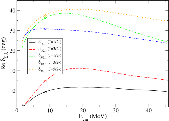
Figure 1: The $p$-wave partial phase shifts for the elastic $nd$ scattering obtained within the WP approach (solid curves) and within the standard Faddeev calculations (circles) [2].

In Fig. 1 the $p$-wave partial phase shifts $\delta^{J\pi}_{\Sigma\lambda}$ of the elastic $nd$ scattering for the Nijmegen I $NN$ potential [14] both below and above a three-body breakup threshold are shown. Here $J$, $\pi$ and $\Sigma$ are the total angular momentum, parity and total channel spin respectively while $\lambda$ is the neutron orbital momentum. The calculation of the phase shifts at 100 different energy values displayed in Fig. 1 takes in our approach (in CPU realization) only about twice as much time as compared with the calculation for a single energy because for all energies we employ the same permutation matrix $\mathbb{P}$ which is calculated only once.

In the next section we consider the specific features related to GPU adaptation for the above numerical scheme.

4 GPU acceleration in calculation of kernel matrix elements

As was noted above, the calculation of elements of a large matrix looks to be very suitable task for effective application of GPU computing if these elements are calculated independently from each other and by one code. However, there are a number of aspects associated with the organization of the data transfer from RAM to the GPU memory and back and also with the GPU computation itself. These aspects impose severe restrictions on the resulting acceleration in GPU realization. One can introduce the GPU acceleration $\eta$ as a ratio of runtime for one-thread CPU computation to runtime for the multithread GPU computation:

$$\eta=t_{\rm CPU}/t_{\rm GPU},$$ (25)

This acceleration depends on the ratio of the actual time for the calculation of one matrix element, $t_{0}$, to the time of transmitting the result from the GPU memory back to RAM, on the number of GPU cores and their speed as compared to speed of CPU core, and also on the dimension of the matrix $M$. Note that the transition itself from a one-thread computing to multithread computing takes some time, so that any parallelization is not effective for matrices with low dimension. When using the GPU, one has to take into account that the speed of GPU cores are usually much smaller than the CPU speed. For the efficiency of multithread computing it is also necessary that the calculations in all threads are finished at approximately the same time. Otherwise a part of threads, each of which occupies a physical core, will be idle for some time. In the case of independent matrix elements, this condition means that the numerical code for one element should not depend on its number, in particular, the code must not contain conditional statements that can change the amount of computation.

When calculating the permutation matrix ${\mathbb{P}}^{0}$ in our algorithm, the above condition is not valid: only about 1% of its non-vanishing matrix elements should be really calculated using a double numerical integration, while other 99% of elements are equal to zero and their determination requires only a few arithmetic operations. Therefore, when one fills the whole matrix ${\mathbb{P}}^{0}$ (including both zero and nonzero elements) 99% of all threads are idle, and we will not reach any real acceleration. Thus we have to develop at first a numerical scheme to fill effectively sparse matrices using GPU.

4.1 GPU acceleration in calculating elements of a sparse matrix

In this subsection in order to check the possibility of GPU acceleration in the calculation of the elements of a matrix with a dimension $M$, we consider two simple examples in which the matrix elements are determined by the following formulas:
(a) as a sum of simple functions:

$$A(i,j)=\sum_{k=1}^{K}\left(\sin^{k}(u_{ij})+\cos^{k}(w_{ij})\right),{\rm or}$$ (26)

(b) as a sum of numerical integrals:

$$A(i,j)=\sum_{k=1}^{K}\int_{u_{ij}}^{w_{ij}}\left(\sin^{k}(t)+\cos^{k}(t)\right)dt.$$ (27)

Here $u_{ij}$ and $w_{ij}$ are random numbers from the interval $[0,1]$ and the parameter $K$ allows to vary the time $t_{0}$ for calculation of each element in a wide range. The integrals in eq. (27) are calculated numerically by the 48-point Gaussian quadrature. Therefore the example (b) with numerical integration is closer to our case of calculating the permutation matrix ${\mathbb{P}}^{0}$ in the Faddeev kernel.

Figures 2, 3 and 4 show the dependence of the GPU acceleration $\eta$ on the matrix dimension $N$ and the calculation time for each element $t_{0}$ when filling up the dense matrices defined by eqs. (26) and (27). The GPU calculations were performed using $M^{2}$ threads, so that, each thread evaluates only one matrix element.

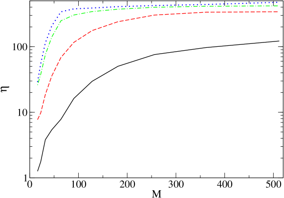
Figure 2: The dependence of GPU acceleration $\eta$ in calculation of elements of dense matrix (26) on the matrix dimension $M$ for different values of $t_{0}$: 0.0009 ms (solid curve), 0.0094 ms (dashed curve), 0.094 ms (dot-dashed curve), 0.94 ms (dotted curve).

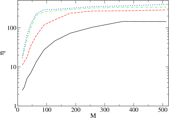
Figure 3: The dependence of GPU acceleration $\eta$ in calculation of elements of a dense matrix (27) on the matrix dimension $M$ for different values of $t_{0}$: 0.0017 ms (solid curve), 0.012 ms (dashed curve), 0.114 ms (dot-dashed curve), 1.13 ms (dotted curve).

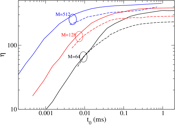
Figure 4: The dependence of GPU acceleration $\eta$ in calculation of elements of dense matrix on the computational time of each matrix element, $t_{0}$, for different values of matrix dimension $M$: solid curves correspond to calculation of matrix elements using simple trigonometric functions (26), dashed curve — using numerical integrals (27).

The calculations are performed on a desk PC with the processor i7-3770K (3.50GHz) and the video card NVIDIA GTX-670. We use the Portland Group Fortran compiler 12.10 including CUDA support and CUDA compiler V5.5. As can be seen from the figures, GPU acceleration sufficiently rises with increasing the dimension $M$ and the computational time for one matrix element $t_{0}$. The maximal acceleration that can be reached in this model example is 400-450(!) Such high degree of acceleration is achieved at the matrix dimension $M\sim 200$ and $t_{0}\gtrsim 0.1$ ms. At further increase of the dimension $M$, the degree of acceleration does not change because in this case all the computing resources of the GPU are already exhausted. Note that, for the example (b) with the numerical integration, the GPU acceleration is somewhat lower than in the case of calculating simple functions. This is due to repeated use of the some constants (the values of the quadrature points and weights) which should be stored in the global GPU memory.

It should also be noted that the transition to the double-precision calculations of the matrix elements reduces greatly the maximal possible value of GPU acceleration $\eta$.

Consider now what efficiency of GPU computing can be reached in the case of a sparse matrix, when it is actually required to calculate only part of matrix elements. We introduce the following additional condition for the matrix elements (26) and (27):

$$\tilde{A}(i,j)=\left\{\begin{array}[]{cc}A(i,j),&u_{ij}\leq\alpha\\ 0,&u_{ij}>\alpha\end{array}\right..$$ (28)

Since $u_{ij}$ is a random number in the interval $[0,1]$, then one gets a sparse matrix with the degree of a sparseness $\sim\alpha$ as a result of such filtration. In fact, the degree of a sparseness is the ratio of number of non-zero matrix elements to their total number $M^{2}$.

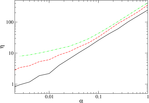
Figure 5: The dependence of GPU acceleration $\eta$ in calculation of elements of sparse matrix with elements (28) on sparseness parameter $\alpha$: solid curve — for $M=64$ dashed curve — for $M=128$ solid curve — for $M=256$.

Fig. 5 shows the dependence of the GPU acceleration on the sparseness parameter $\alpha$ in filling matrices with dimensions $M=64$, 128 and 256. As can be seen from the Figure, the GPU acceleration is only about 2 (for $M=64$) at a value of $\alpha\sim 0.01$, which corresponds to the realistic sparseness parameter for the permutation matrix ${\mathbb{P}}^{0}$ in the Faddeev kernel.

Thus, to achieve a significant GPU acceleration in calculating the permutation matrix ${\mathbb{P}}^{0}$, it is necessary to add one more step to our numerical scheme discussed in the section 3.3 and perform a pre-selection of nonzero elements of the permutation matrix.

4.2 The GPU algorithm for calculating the permutation matrix in the case of a semi-realistic $s$-wave $NN$ interaction

Consider now a calculation of the permutation matrix ${\mathbb{P}}^{0}$ entering the Faddeev kernel. There are additional limitations for the GPU algorithm for this case compared to simple examples discussed in the previous subsection.

a) As already mentioned above, the most serious limitations are a high dimension and a high sparseness of the permutation matrix, and therefore a special packaging for this matrix is required. Standard packaging for a matrix (we use the packaging on the rows — the so called CSR format) implies, instead of storing the matrix in a single array ${A}$ with a dimension $M\times M$, the presence of two linear arrays, ${B}$ and ${C}$, with dimensions $\alpha M^{2}$, which store the nonzero matrix elements of ${A}$ and the respective numbers of columns. Also the third linear array ${W}$ with the dimension $M$ contains addresses of the last nonzero elements (in the array ${B}$), corresponding to a given row of the initial matrix ${A}$. With such a way of the matrix packaging we get a gain in the memory required for storing the matrix to be equal to $1/(2\alpha)$, i.e. about 50-fold gain for a value of the sparseness 0.01 which is specific for the permutation matrix $\mathbb{P}^{0}$ in the WP representation. So that, at the specific matrix dimension $M\sim 5\cdot 10^{5}$ which is necessary for an accurate calculation of the realistic $3N$ scattering problem, the whole matrix occupies about 1,000 GB of RAM (with single precision), while the same matrix in a compressed form takes about 20 GB RAM only. This is a quite acceptable value for a modern desktop computer.

b) However, the permutation matrix of such a dimension, even in a packed form, cannot be placed in the GPU memory which is usually 4-8 GB only. Therefore one needs to subdivide the whole calculation of this matrix into some blocks using an external CPU cycle and then employ the multithread GPU computation for each block.

c) Another distinction of the calculation of the elements of the matrix ${\mathbb{P}}^{0}$ from the simple model example discussed above is the necessity to use a large number of constants: in particular, the values of nodes and weights for Gaussian quadratures for a calculation of double integrals and also (in case of a realistic $NN$ interaction with tensor components) algebraic coefficients $g^{\Gamma\alpha\beta,\alpha^{\prime}\beta^{\prime}}_{\gamma,\gamma^{\prime}}$ from the eq. (22) for coupling of different spin-angular channels, values of Legendre polynomials at the nodal points etc. All these data are stored in the global GPU memory and because of the relatively low access rate of each thread to the global GPU memory, the resulted acceleration is noticeably lower than in the case of the above simple code which does not use a large amount of data from the global GPU memory.

d) The necessary pre-selection of nonzero elements of the matrix ${\mathbb{P}}^{0}$ can be itself quite effectively parallelized for a GPU implementation. Since the runtime for checking the selection criteria for each element is on two orders of magnitude less than the runtime for calculating nonzero element itself, then the degree of GPU acceleration for the stage of a pre-selection turns out less than for the basic calculation. Nevertheless, if do not employ the GPU at this stage, the computing time for it turns out even larger than the GPU calculation time for all nonzero elements (see below).

After these general observations, we describe the results for the GPU computing of the most tedious step of solving the Faddeev equation in the WP approach — the computation of nonzero elements of the permutation matrix — in the case of a semi-realistic Malfliet-Tjon $NN$ interaction. There is no spin-angular coupling for this potential, so that the Faddeev system is reduced to a single $s$-wave equation. The results attained for a realistic calculation of multichannel $nd$ scattering we leave for the next section.

When the pre-selection of nonzero matrix elements is already done one has the subsidiary arrays ${C}$ and ${W}$ containing information about all nonzero elements of $\mathbb{P}^{0}$ that should be calculated and the number of these nonzero elements is $M_{t}$. The parallelization algorithm adapted here assumes that every matrix element is computed by a separate thread. The allowable number of threads $N_{\rm thr}$ is restricted by the capacity of the physical GPU memory and is usually less than the total number of nonzero elements $M_{t}$. In this case, our algorithm consists of the following steps.

1. The data used in calculation (endpoints of momentum intervals in variables $p$ and $q$, nodes and weights of Gauss quadratures, algebraic coupling coefficients etc.) are copied to the GPU memory.

2. The whole set of nonzero elements of the permutation matrix is divided into $N_{b}$ blocks with $N_{\rm thr}$ elements in each block (except the last one) and the external CPU loop is organized by the number of such blocks. Inside the loop the following operations are performed:

3. A part of the array ${C}$ corresponding to the current block is copied to the GPU memory.

4. The CUDA-kernel is launched on GPU in $N_{\rm thr}$ parallel threads each of which calculates only one element (in the case of the $s$-wave problem) of the permutation matrix.

5. The resulted $N_{\rm thr}$ nonzero elements of the matrix are copied from the GPU memory to the appropriate place of the total array ${B}$.

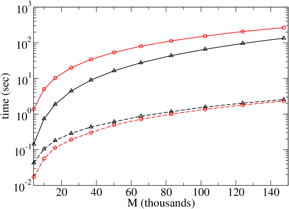
Figure 6: The CPU computing time (solid curves) and GPU computing time (dashed curves) for preselection of tne nonzero elements of $s$-wave permutation matrix ${\mathbb{P}}^{0}$ (triangles) and calculation of these elements (circles) depending on the matrix dimension $M$.

Fig. 6 shows the dependence of the CPU- and GPU-computing time for the calculation of the $s$-wave permutation matrix upon its total dimension $M=N\times\bar{N}$ (for $N=\bar{N}$). In our case, the GPU code was executed in 65536 threads. For the comparison, we display on this Figure also the CPU and GPU time which are necessary for a pre-selection of nonzero matrix elements. It is clear from the Figure that one needs to use GPU computing not only for the calculation of nonzero elements (that takes most of the time in one-thread CPU computing), but also for the pre-selection of nonzero matrix elements to achieve a high degree of the acceleration.

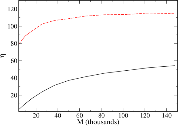
Figure 7: The dependence of the GPU acceleration $\eta$ on the matrix dimension $M$ for a calculation of the permutation matrix (dashed curve) and for a complete solution of the scattering problem (solid curve) in the case of $s$-wave $NN$ interaction.

In Fig. 7, we present the GPU acceleration $\eta$ for calculating the $s$-wave permutation matrix and for a complete solution of $s$-wave $nd$ elastic scattering problem on dimension $M$ of the matrix equation. It is evident that the runtime for the nonzero elements of the matrix ${\mathbb{P}}^{0}$ (which takes the main part of the CPU computing time) is reduced by more than 100 times. The total acceleration in calculating the $s$-wave partial phase shifts reaches 50. Finally, the total three-body calculation takes only 7 sec. on an ordinary PC with GPU.

5 GPU optimization for a realistic $3N$ scattering problem

5.1 GPU-acceleration for a realistic $nd$ scattering amplitude

We now turn to the case of a realistic three-nucleon scattering problem with the Nijmegen I $NN$ potential [14] and the calculation for the elastic $nd$ scattering cross section.

Unlike the simple $s$-wave case discussed above, now we have many coupled spin-angular channels (up to 62 channels if the total angular momentum in $NN$ pair is restricted as $j\leq 3$). In this case, the calculation of each element of the permutation matrix ${\mathbb{P}}^{0}$ comprises the calculation of several tens of double numerical integrals containing the Legendre polynomials. Each matrix element is equal to the sum of such double integrals and the sum includes a large set of algebraic coupling coefficients $g^{\Gamma\alpha\beta,\alpha^{\prime}\beta^{\prime}}_{\gamma,\gamma^{\prime}}$ for the spin-angular channels as in eq. (22).

Now the GPU-optimized algorithm for the permutation matrix is somewhat different: because each calculated double integral is used to compute several matrix elements, then each thread now calculates all the matrix elements corresponding to one pair of momentum cells $\{\mathfrak{D}_{ij},\mathfrak{D}_{i^{\prime}j^{\prime}}\}$. These matrix elements belong to different rows of the complete permutation matrix. So that, after the GPU computing for each block of the permutation matrix it is necessary to rearrange and repack (in the single-thread CPU execution) the calculated set of the matrix elements into the arrays ${B}$, ${C}$ and ${W}$, representing the complete matrix $\mathbb{P}^{0}$ in CSR format. All the above leads to the fact that the GPU acceleration in calculation of the permutation matrix in a realistic case when the $NN$ interaction has a tensor component turns out significantly less than for the $s$-wave case.

Fig. 8 demonstrates the GPU acceleration $\eta$ versus the basis dimension $M=N\times\bar{N}$ in the solution of 18-channel Faddeev equation for the partial $nd$ elastic amplitude with total angular momentum $J=\frac{1}{2}^{+}$ (solid line). The dashed and dot-dashed lines show the GPU acceleration for stage of pre-selection of nonzero elements for the permutation matrix ${\mathbb{P}}^{0}$ and for calculating of these elements, respectively.

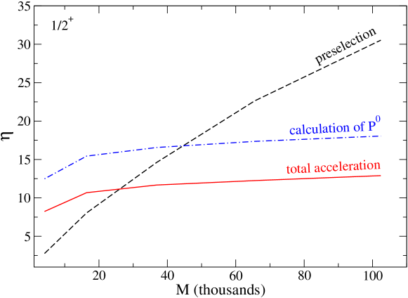
Figure 8: The dependence of the GPU acceleration $\eta$ on dimension of the basis $M=N\times\bar{N}$ (for the case $N=\bar{N}$) for the realistic $nd$ scattering problem at $J=\frac{1}{2}^{+}$: dashed line shows the acceleration for the preselection of nonzero elements in the permutation matrix ${\mathbb{P}}^{0}$), dot-dashed line – for the calculation of these elements, solid line – the acceleration for the complete solution.

From these results, it is evident that the acceleration in the calculation of the coupled-channel permutation matrix is about 15 that is considerably less in comparison with the above one-channel $s$-wave case. Nevertheless, the passing from CPU- to GPU-realization on the same PC allows to obtain a quite impressive acceleration about 10 in the solution of the 18-channel scattering problem.

In realistic calculation of the observables for elastic $nd$ scattering, it is necessary to include up to 62 spin-orbital channels. For the current numerical scheme, the efficiency of GPU optimization decreases with increasing number of channels. As an example, we present the results of the complete calculation for elastic $nd$ scattering with the Nijmegen I $NN$ potential at energy 22.7 MeV. In Fig. 9 as an illustration of an accuracy of our approach, we display the differential cross section in comparison with the results of the conventional approach [2].

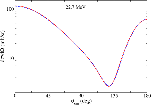
Figure 9: The differential cross section of elastic $nd$ scattering at energy 22.7 MeV calculated with the Nijmegen I $NN$ potential in wave-packet formalism with using GPU computing (solid curve) in comparison with the results from the ref. [2] (dashed curve).

The complete calculation, including 62 spin-orbital channels and all states with total angular momentum up to $J_{\rm max}=17/2$ took about 30 min on our desk PC. The runtimes for separate steps are given in Table 1.

Table 1: Runtime (in sec) for separate steps of complete solutions of $nd$ scattering problem

	Step	CPU time	GPU time
1.	Processing input data	30	30
2a.	Pre-selection	12	1.9
2b.	Calculation of nonzero elements	4558	524
4.	Iterations and Pade summation	1253	1250
	Total time	5852	1803

As seen from the Table, the time of calculation of the permutation matrix elements (steps 2a and 2b) is shorten in ca. 8.7 times as a result of the GPU optimization. However, the major part of a computational time is now spent not on calculating the permutation matrix but on the subsequent iterations of the resulting matrix equation, i.e. on multiplication of a kernel matrix by a column of current solution. The iteration time takes about 69% of total solution time. So that, the total acceleration in this multichannel case is only 3.2.

It should be stressed that the current numerical scheme can be further optimized. Each iteration here includes four matrix multiplications: one multiplication by a diagonal matrix $\mathbb{G}_{1}$, two multiplications by block matrices $\mathbb{O}$ and $\tilde{\mathbb{V}}_{1}$ and one multiplication by sparse matrix $\mathbb{P}^{0}$, and most of the time in the iteration process takes multiplication of a sparse matrix by a (dense) vector. It is clear that the algorithm for the iteration can also be parallelized and implemented on the GPU. In this paper, we did not addressed this task and focused mainly on the GPU optimization for the calculation the integral kernel of Faddeev equation only. However, for a multiplication of a sparse matrix to a column there are standard procedures, including those implemented on GPU. So that, if to apply the GPU optimization to the iteration step the runtime of complete solution can be reduced further by 2-3 times.

It is also clear that employment of more powerful specialized graphics processors would lead even to a considerably greater acceleration of the calculations.

5.2 Further development

It looks evident that the described GPU approach will be effective also in the solution of integral equations describing the scattering in systems of four and a larger number of particles (Faddeev–Yakubovsky equations). The main difference in these more complicated problems from the three-body scattering problem considered here is increasing number of channels to be included and also rising of the dimension for integrals those define the kernel matrix elements. As the result, the matrix dimension $M$ and the computational time of each matrix element $t_{0}$ will increase. However, a degree of sparseness for the permutation matrices and scheme for calculation of kernel matrix elements will remain the same as in a three-body case. So that, these two factors, i.e. growth of $M$ and $t_{0}$, according to our results, will provide even greater GPU acceleration than in a three-body case.

However, when the matrix size $M$ will reach a certain limit, no package will be able to place all nonzero elements in RAM of a computer. In such a case, it should be chosen another strategy: one divides the channel space onto two parts: the major and minor channels according to their influence to the resulted amplitude. The minor channels would give only a small correction contribution to the solution resulting from the subspace of the major channels. Then, using the convenient projection formalism (such as the known Feshbach formalism), one can account for the minor-channel contribution in a matrix kernel defined in the subspace of the major channels as some additional effective interaction containing the total resolvent in the minor-channel subspace. We have shown previously [10, 15] that the basis dimension for the minor channels can be considerably reduced (for a particular problem, it can be reduced in 10 times [15]) without loss in an accuracy of a complete solution.

We hope that such a combined approach together with the multithread GPU computing will lead to the greater progress in the exact numerical solution of quantum few-body scattering problems when using a desktop PC.

6 Conclusion

In the present paper we have checked the applicability of the GPU-computing technique in few-body scattering calculations. For this purpose we have used the wave-packet continuum discretization approach in which a continuous spectrum of the Hamiltonian is approximated by a discrete spectrum of the $L_{2}$ normalizable wave-packet states. If to project out all the wave functions and scattering operators onto such a discrete basis we arrive at simple linear matrix equation with non-singular matrix elements instead of the complicated multi-dimensional singular equations in the initial formulation of few-body scattering problem. Moreover, the matrix elements of all the constituents of this equation are calculated independently which make the numerical scheme to be highly parallelized.

The prize for this matrix reduction is a high dimension for the matrix kernel. In the case of fully realistic problem the dimension of the kernel matrix turns out so high that such a matrix cannot be placed into RAM of a desktop PC. In addition the calculation of all kernel matrix elements requires a huge computing time in sequential one-thread execution. However, we have developed efficient algorithms of parallelization, which allows to perform basic calculations in the multithread GPU execution and reach a noticeable acceleration of calculations.

It is shown that the acceleration obtained due to GPU-realization depends on the dimension of the basis used and the complexity of the problem. So, in the three-body problem of the elastic $nd$ scattering with a semi-realistic $s$-wave $NN$ interaction, we obtained 50-fold acceleration for the whole solution while for a separate part of the numerical scheme (most time consuming on CPU) the acceleration achieves more than 100 times. In a case of the fully realistic $NN$ interaction for the $nd$ scattering (including up to 62 spin-orbit channels), the acceleration for the permutation matrix calculation is about 8.7 times. A full calculation of the differential cross section is accelerated in this case by 3.2 times. However, the numerical scheme allows a subsequent optimization that will be done in our further investigations. Nevertheless, the present study has shown that the implementation of GPU calculations in few-body scattering problems is very perspective at all and opens new possibilities for a wide group of researches.

It should be stressed, the developed GPU accelerated discrete approach to solution of quantum scattering problems can be transferred without major changes to other areas of quantum physics, as well as to a number of important areas of classical physics involving solution of multidimensional problems for continuous media studies.

Acknowledgments This work has been supported partially by the Russian Foundation for Basic Research, grant No. 13-02-00399.

References

- [1] H. Witała, W.Glöckle, Phys. Rev. C 85 (2012) 064003.
- [2] W. Glöckle, H. Witała, D.Hüber, H. Kamada, J. Golack, Phys. Rep. 274 (1996) 107.
- [3] J. Carbonell, A. Deltuva, A.C. Fonseca, R. Lazauskas, Progr. Part. Nucl. Phys. 74 (2014) 55.
- [4] https://developer.nvidia.com/cuda-zone
- [5] B. Block, P. Virnau, T. Preis, Comp. Phys. Com. 181 (2010) 1549.
- [6] M.A. Clark, R. Babich, K. Barrose, R.C. Brower, C. Rebbi, Comp. Phys. Com. 181 (2010) 1517.
- [7] K.A. Wilkinson, P. Sherwood, M.F. Guest, K.J. Naidoo, J. Comp. Chem. 32 (2011) 2313.
- [8] H. Potter et al., in Proceedings of NTSE-2013 (Ames, IA, USA, May 13-17, 2013), edited by A. M. Shirokov and A. I. Mazur, Khabarovsk, Russia, 2014, p. 263. http://www.ntse-2013.khb.ru/Proc/Sosonkina.pdf.
- [9] E. Yarevsky, LNCS 7125, Mathematical Modeling and Computational Science, Eds. A. Gheorghe, J. Buša and M. Hnatic, 2012, p. 290.
- [10] O.A. Rubtsova, V.I. Kukulin, V.N. Pomerantsev, Ann. Phys. 360 (2015) 613.
- [11] O.A. Rubtsova, V.N. Pomerantsev, V.I. Kukulin, A. Faessler, Phys. Rev. C 86 (2012) 034004.
- [12] S.A. Kelvich, V.I. Kukulin, O.A. Rubtsova, Physics of Atomic Nuclei 77 (2014) 438.
- [13] V.N. Pomerantsev, V.I. Kukulin, O.A. Rubtsova, Phys. Rev. C 89 (2014) 064008.
- [14] V.G.J. Stoks, R.A.M. Klomp, C.P.F. Terheggen, J.J de Swart, Phys. Rev. C 49 (1994) 2950.
- [15] O.A. Rubtsova, V.I. Kukulin, Phys. At. Nucl. 70 (2007) 2025.