Subdifferential-based implicit return-mapping operators in Mohr-Coulomb plasticity

Abstract

The paper is devoted to a constitutive solution, limit load analysis and Newton-like methods in elastoplastic problems containing the Mohr-Coulomb yield criterion. Within the constitutive problem, we introduce a self-contained derivation of the implicit return-mapping solution scheme using a recent subdifferential-based treatment. Unlike conventional techniques based on Koiter’s rules, the presented scheme a priori detects a position of the unknown stress tensor on the yield surface even if the constitutive solution cannot be found in closed form. This fact eliminates blind guesswork from the scheme, enables to analyze properties of the constitutive operator, and simplifies construction of the consistent tangent operator which is important for the semismooth Newton method applied on the incremental boundary value elastoplastic problem. The incremental problem in Mohr-Coulomb plasticity is combined with the limit load analysis. Beside a conventional direct method of the incremental limit analysis, a recent indirect one is introduced and its advantages are described. The paper contains 2D and 3D numerical experiments on slope stability with publicly available Matlab implementations.

Keywords: infinitesimal plasticity, Mohr-Coulomb yield surface, implicit return-mapping scheme, consistent tangent operator, semismooth Newton method, incremental limit analysis, slope stability

1 Introduction

This paper is a continuation of [1] which was devoted to a solution of elastoplastic constitutive problems using a subdifferential formulation of the plastic flow rule. It leads to simpler and more correct implicit constitutive solution schemes. While a broad class of elastoplastic models containing 1 or 2 singular points (apices) on the yield surface was considered in [1], the aim of this paper is to approach the subdifferential-based treatment to models that are usually formulated in terms of principal stresses. For example, the principal stresses are used in models containing the Mohr-Coulomb, the Tresca, the Rankine, the Hoek-Brown or the unified strength yield criteria [2, 3, 4, 5]. Such criteria have a multisurface representation leading to a relatively complex structure of singular points.

Due to technical complexity of implicit solution schemes for these models, we focus only on a particular but representative yield criterion: the Mohr-Coulomb one. This criterion is broadly exploited in soil and rock mechanics and its surface is a hexagonal pyramid aligned with the hydrostatic axis (see, e.g., [2]). We consider the Mohr-Coulomb model introduced in [2, Section 8] which can optionally contain the nonassociative flow rule and the nonlinear isotropic hardening. The nonassociative flow rule enables to catch the dilatant behavior of a material. Further, due to the presence of the nonlinear hardening, one cannot find the implicit constitutive solution in closed form, and thus the problem remains challenging. As in [2], we let a hardening function in an abstract form. For a particular example of the nonlinear hardening in soil mechanics, we refer, e.g., [6].

In literature, there are many various concepts of the constitutive solution schemes for models containing yield criteria written in terms of the principal stresses. For their detailed overview and historical development, we refer the recent papers [3] and [7], respectively. It is worth mentioning that the solution schemes mainly depend on a formulation of the plastic flow rule, its discretization and other eventual approximations.

In engineering practice, the plastic flow rule is usually formulated using the so-called Koiter rule introduced in [8] for associative models with multisurface yield criteria. Consequently, this rule was also extended for nonassociative models, see, e.g., [9]. It consists of several formulas that depend on a position of the unknown stress tensor $\sigma$ on the yield surface. The formulas have a different number of plastic multipliers. Within the Mohr-Coulomb pyramid, one plastic multiplier is used for smooth portions, two multipliers at edge points, and six multipliers at the apex. For each Koiter’s formula, a different solution scheme is introduced. However, only one of which usually gives the correct stress tensor. Moreover, the handling with different numbers of plastic multipliers is not suitable for analysing the stress-strain operator even if the solution can be found in closed form. If an elastoplastic model contains a convex plastic potential as the Mohr-Coulomb one then it is possible to replace the Koiter rule with a subdifferential of the potential (see, e.g., [2]). Such a formulation is independent of the unknown stress position, contains just one plastic multiplier, and thus it is more convenient for mathematical analysis of the constitutive operators. In [1], it was shown that this formulation is also convenient for a solution of some constitutive problems. Further, in some special cases, the constitutive problem can be also defined using the principle of maximum plastic dissipation [2, 10] or by the theory of bipotentials [11] and solved by techniques based on mathematical programming.

We focus on the (fully) implicit Euler discretization of the flow rule, which is frequently used in elastoplasticity. Beside other Euler-type methods (see, e.g., [2, 12]), the cutting plane methods are also popular. We refer, e.g., [13] for the literature survey and recent development of these methods. When the constitutive problems are discretized by the implicit Euler methods, the solution is searched by the elastic predictor – plastic correction method. Within the plastic correction, the so-called (implicit) return-mapping scheme is constructed. It is worth mentioning that plastic correction problems can be reduced to problems formulated only in terms of the principal stresses [14, 3, 2].

In order to simplify the solution schemes for nonsmooth yield criteria, many various approximative techniques have been suggested. These techniques are based on local or global smoothing of yield surfaces or plastic potentials. For literature survey, we refer [3, Section 1.2] or [15, 16, 6]. However, such an approach is out of the scope of this paper.

The constitutive problem is an essential part of the overall initial boundary value elastoplastic problem. Its time discretization leads to the incremental boundary value problem which is mostly solved by nonsmooth variants of the Newton method [17, 18, 19, 20, 21] in each time step. Then, it is useful to construct the so-called consistent tangent operator representing a generalized derivative of the discretized constitutive stress-strain operator. We use the framework based on the eigenprojections of symmetric second order tensors, see, e.g., [22, 2]. A similar approach is also used in the recent book [16] with slightly different terminology like the spectral directions or the spin of a tensor. Another approach is introduced, e.g., in [23, 14, 3] where the consistent tangent operator is determined by the tangent operator representing the relation between the stress and strain rates.

Further, this paper is devoted to the limit load problem which is frequently combined with the Mohr-Coulomb model. It is an additional problem to the elastoplastic one where the load history is not fully prescribed. It is only given a fixed external force that is multiplied by a scalar load parameter whose limit value is unknown. It is well known that the investigated body collapses when this critical value is exceeded. Therefore, this value is an important safety parameter and beyond it no solution exists. Strip-footing collapse or slope stability are traditional applications on this problematic (see, e.g. [24, 2]). The simplest computational technique is based on the so-called incremental limit analysis where the load parameter is enlarged up to its limit value. Then, the boundary-value elastoplastic problem is solved for investigated values of this parameter. Beside the conventional direct method of the incremental limit analysis, we also introduce the indirect method and describe its advantages based on recent expertise introduced in [25, 26, 27, 28].

The rest of the paper is organized as follows. In Section 2, an auxilliary framework related to the subdifferential of an eigenvalue function and derivatives of eigenprojections is introduced. In Section 3, the Mohr-Coulomb constitutive initial value problem is formulated using the subdifferential of the plastic potential and discretized by the implicit Euler method. In Section 4, the existence and uniqueness of a solution to the discretized problem is proven and the improved solution scheme is derived. In Section 5, the stress-strain and the consistent tangent operators are constructed. In Section 6, the direct and indirect methods of the incremental limit analysis are introduced. Both methods are combined with the semismooth Newton method. In Section 7, 2D and 3D numerical experiments related to slope stability are introduced. In Section 8, some concluding remarks are mentioned. The paper also contains Appendix with some useful auxilliary results. In Appendix A, the solution scheme is simplified under the plane strain assumptions. In Appendix B, algebraic representations for second and fourth order tensors within the 3D and plane strain problems are derived.

In this paper, second order tensors, matrices, and vectors are denoted by bold letters. Further, the fourth order tensors are denoted by capital blackboard letters, e.g., $\mathbb{D}_{e}$ or $\mathbb{I}$. The symbol $\otimes$ means the tensor product [2]. We also use the following notation: $\mathbb{R}_{+}:=\{z\in\mathbb{R};\;z\geq 0\}$ and $\mathbb{R}^{3\times 3}_{sym}$ for the space of symmetric, second order tensors. The standard scalar product in $\mathbb{R}^{3}$ and the biscalar product in $\mathbb{R}^{3\times 3}_{sym}$ are denoted as $\cdot$ and $:$, respectively.

2 Subdifferentials and derivatives of eigenvalue functions

In this section, we introduce an auxilliary framework that will be crucial for an efficient construction of the constitutive and consistent tangent operators in Mohr-Coulomb plasticity. Let

$$\mbox{\boldmath$\eta$}=\sum_{i=1}^{3}\eta_{i}\mathbf{e}_{i}\otimes\mathbf{e}_{i},\quad\eta_{1}\geq\eta_{2}\geq\eta_{3},$$ (2.1)

be the spectral decomposition of a tensor $\mbox{\boldmath$\eta$}\in\mathbb{R}^{3\times 3}_{sym}$. Here, $\eta_{i}\in\mathbb{R}$, $\mathbf{e}_{i}\in\mathbb{R}^{3}$, $i=1,2,3$, denote the eigenvalues, and the eigenvectors of $\eta$, respectively. The eigenvalues $\eta_{1},\eta_{2},\eta_{3}$ can be computed using the Haigh-Westargaard coordinates (see, e.g., [2, Appendix A]), and they are uniquely determined with respect to the prescribed ordering. Let $\omega_{1},\omega_{2},\omega_{3}$ denote the corresponding eigenvalue functions, i.e. $\eta_{i}:=\omega_{i}(\mbox{\boldmath$\eta$})$, $i=1,2,3$. Further, we define the following set of admissible eigenvectors of $\eta$:

$$V(\mbox{\boldmath$\eta$})=\{(\mathbf{e}_{1},\mathbf{e}_{2},\mathbf{e}_{3})\in\mathbb{R}^{3}\times\mathbb{R}^{3}\times\mathbb{R}^{3}\ |\;\mathbf{e}_{i}\cdot\mathbf{e}_{j}=\delta_{ij};\;\mbox{\boldmath$\eta$}\mathbf{e}_{i}=\eta_{i}\mathbf{e}_{i},\;i,j=1,2,3;\;\eta_{1}\geq\eta_{2}\geq\eta_{3}\}.$$

2.1 Subdifferential of an eigenvalue function

Recall the definition of the subdifferential to a convex function $g:\mathbb{R}^{3\times 3}_{sym}\rightarrow\mathbb{R}$ at $\eta$:

$$\partial g(\mbox{\boldmath$\eta$})=\{\mbox{\boldmath$\nu$}\in\mathbb{R}^{3\times 3}_{sym}\ |\;g(\mbox{\boldmath$\tau$})\geq g(\mbox{\boldmath$\eta$})+\mbox{\boldmath$\nu$}:(\mbox{\boldmath$\tau$}-\mbox{\boldmath$\eta$})\;\;\forall\mbox{\boldmath$\tau$}\in\mathbb{R}^{3\times 3}_{sym}\}.$$

To receive the Mohr-Coulomb yield function or the plastic potential, we specify $g$ as follows:

$$g(\mbox{\boldmath$\eta$})=a\omega_{1}(\mbox{\boldmath$\eta$})-b\omega_{3}(\mbox{\boldmath$\eta$}),\quad\mbox{\boldmath$\eta$}\in\mathbb{R}^{3\times 3}_{sym},$$ (2.2)

where the parameters $a,b\geq 0$ are sufficiently chosen. Notice that the convexity of the eigenvalue function $g$ can be derived from:

$$\omega_{1}(\mbox{\boldmath$\eta$})=\max_{\begin{subarray}{c}\mathbf{e}\in\mathbb{R}^{3}\\ |\mathbf{e}|=1\end{subarray}}\mbox{\boldmath$\eta$}:(\mathbf{e}\otimes\mathbf{e})=\max_{\begin{subarray}{c}\mathbf{e}\in\mathbb{R}^{3}\\ |\mathbf{e}|=1\end{subarray}}\ (\mbox{\boldmath$\eta$}\mathbf{e})\cdot\mathbf{e},\quad\omega_{3}(\mbox{\boldmath$\eta$})=\min_{\begin{subarray}{c}\mathbf{e}\in\mathbb{R}^{3}\\ |\mathbf{e}|=1\end{subarray}}\mbox{\boldmath$\eta$}:(\mathbf{e}\otimes\mathbf{e}).$$ (2.3)

Specific form of $\partial g(\mbox{\boldmath$\eta$})$ with respect to (2.2) can be found using a framework introduced in [29, Chapter 2]. We derive another form of $\partial g(\mbox{\boldmath$\eta$})$ that is convenient for purposes of this paper.

Lemma 2.1.

Let $g:\mathbb{R}^{3\times 3}_{sym}\rightarrow\mathbb{R}$ be defined by (2.2). Then for any $\mbox{\boldmath$\eta$}\in\mathbb{R}^{3\times 3}_{sym}$, it holds:

$$\partial g(\mbox{\boldmath$\eta$}) = \left\{\mbox{\boldmath$\nu$}=\sum_{i=1}^{3}\nu_{i}\mathbf{e}_{i}\otimes\mathbf{e}_{i}\in\mathbb{R}^{3\times 3}_{sym}\ |\;(\mathbf{e}_{1},\mathbf{e}_{2},\mathbf{e}_{3})\in V(\mbox{\boldmath$\eta$});\;a\geq\nu_{1}\geq\nu_{2}\geq\nu_{3}\geq-b;\right.$$ (2.4)

$$\quad\left.\sum_{i=1}^{3}\nu_{i}=a-b;\;(\nu_{1}-a)[\omega_{1}(\mbox{\boldmath$\eta$})-\omega_{2}(\mbox{\boldmath$\eta$})]=0;\;(\nu_{3}+b)[\omega_{2}(\mbox{\boldmath$\eta$})-\omega_{3}(\mbox{\boldmath$\eta$})]=0\right\}.$$

Proof.

Since $g(\mbox{\boldmath$0$})=0$ and $g(2\mbox{\boldmath$\eta$})=2g(\mbox{\boldmath$\eta$})$ the standard definition of $\partial g(\mbox{\boldmath$\eta$})$ is equivalent to:

$$\partial g(\mbox{\boldmath$\eta$})=\{\mbox{\boldmath$\nu$}\in\mathbb{R}^{3\times 3}_{sym}\ |\;g(\mbox{\boldmath$\eta$})=\mbox{\boldmath$\nu$}:\mbox{\boldmath$\eta$};\;g(\mbox{\boldmath$\tau$})\geq\mbox{\boldmath$\nu$}:\mbox{\boldmath$\tau$}\;\;\forall\mbox{\boldmath$\tau$}\in\mathbb{R}^{3\times 3}_{sym}\}.$$ (2.5)

First, we derive necessary and sufficient conditions on $\mbox{\boldmath$\nu$}\in\mathbb{R}^{3\times 3}_{sym}$ ensuring

$$g(\mbox{\boldmath$\tau$})\geq\mbox{\boldmath$\nu$}:\mbox{\boldmath$\tau$}\quad\forall\mbox{\boldmath$\tau$}\in\mathbb{R}^{3\times 3}_{sym}.$$ (2.6)

To this end, consider the following spectral decomposition of $\nu$:

$$\mbox{\boldmath$\nu$}=\sum_{i=1}^{3}\nu_{i}\mathbf{f}_{i}\otimes\mathbf{f}_{i},\quad\nu_{1}\geq\nu_{2}\geq\nu_{3},\quad(\mathbf{f}_{1},\mathbf{f}_{2},\mathbf{f}_{3})\in V(\mbox{\boldmath$\nu$}).$$ (2.7)

Choose $\mbox{\boldmath$\tau$}=\pm\mbox{\boldmath$I$}$, where $I$ is the unit tensor in $\mathbb{R}^{3\times 3}_{sym}$. Then from (2.6), (2.7) we have:

$$\nu_{1}+\nu_{2}+\nu_{3}=a-b.$$ (2.8)

Choose $\mbox{\boldmath$\tau$}=\mathbf{f}_{1}\otimes\mathbf{f}_{1}$ and $\mbox{\boldmath$\tau$}=-\mathbf{f}_{3}\otimes\mathbf{f}_{3}$. Then from (2.6), (2.7) we derive, respectively:

$$\nu_{1}\leq a,\quad\nu_{3}\geq-b.$$ (2.9)

Let $\mbox{\boldmath$\tau$}\in\mathbb{R}^{3\times 3}_{sym}$ be arbitrarily chosen and denote $\tau_{i}:=\mbox{\boldmath$\tau$}:(\mathbf{f}_{i}\otimes\mathbf{f}_{i})$, $i=1,2,3$, $(\mathbf{f}_{1},\mathbf{f}_{2},\mathbf{f}_{3})\in V(\mbox{\boldmath$\nu$})$. Then,

$$\tau_{1}+\tau_{2}+\tau_{3}=\mbox{\boldmath$\tau$}:\mbox{\boldmath$I$}=\omega_{1}(\mbox{\boldmath$\tau$})+\omega_{2}(\mbox{\boldmath$\tau$})+\omega_{3}(\mbox{\boldmath$\tau$}),\qquad\omega_{1}(\mbox{\boldmath$\tau$})\geq\tau_{i}\geq\omega_{3}(\mbox{\boldmath$\tau$}),\quad\forall i=1,2,3,$$ (2.10)

follow from $\mbox{\boldmath$I$}=\sum_{i=1}^{3}\mathbf{f}_{i}\otimes\mathbf{f}_{i}$ and (2.3), respectively. Consequently,

$$\mbox{\boldmath$\nu$}:\mbox{\boldmath$\tau$} = \sum_{i=1}^{3}\nu_{i}\tau_{i}=\tau_{1}(\nu_{1}-\nu_{2})+(\tau_{1}+\tau_{2})(\nu_{2}-\nu_{3})+(\tau_{1}+\tau_{2}+\tau_{3})\nu_{3}$$ (2.11)

$$\stackrel{{\scriptstyle(\ref{tau_i_prop})}}{{=}} \tau_{1}(\nu_{1}-\nu_{2})+(\mbox{\boldmath$\tau$}:\mbox{\boldmath$I$}-\tau_{3})(\nu_{2}-\nu_{3})+\nu_{3}\mbox{\boldmath$\tau$}:\mbox{\boldmath$I$}$$

$$\stackrel{{\scriptstyle(\ref{tau_i_prop})}}{{\leq}} \omega_{1}(\mbox{\boldmath$\eta$})(\nu_{1}-\nu_{2})+[\mbox{\boldmath$\tau$}:\mbox{\boldmath$I$}-\omega_{3}(\mbox{\boldmath$\eta$})](\nu_{2}-\nu_{3})+\nu_{3}\mbox{\boldmath$\tau$}:\mbox{\boldmath$I$}=\sum_{i=1}^{3}\nu_{i}\omega_{i}(\mbox{\boldmath$\eta$})$$

$$= \nu_{1}[\omega_{1}(\mbox{\boldmath$\eta$})-\omega_{2}(\mbox{\boldmath$\eta$})]+(\nu_{1}+\nu_{2})[\omega_{2}(\mbox{\boldmath$\eta$})-\omega_{3}(\mbox{\boldmath$\eta$})]+(\nu_{1}+\nu_{2}+\nu_{3})\omega_{3}(\mbox{\boldmath$\eta$})$$

$$\stackrel{{\scriptstyle(\ref{cond_sub_1})}}{{=}} \nu_{1}[\omega_{1}(\mbox{\boldmath$\eta$})-\omega_{2}(\mbox{\boldmath$\eta$})]+(a-b-\nu_{3})[\omega_{2}(\mbox{\boldmath$\eta$})-\omega_{3}(\mbox{\boldmath$\eta$})]+(a-b)\omega_{3}(\mbox{\boldmath$\eta$})$$

$$\stackrel{{\scriptstyle(\ref{cond_sub_2})}}{{\leq}} a[\omega_{1}(\mbox{\boldmath$\eta$})-\omega_{2}(\mbox{\boldmath$\eta$})]+a[\omega_{2}(\mbox{\boldmath$\eta$})-\omega_{3}(\mbox{\boldmath$\eta$})]+(a-b)\omega_{3}(\mbox{\boldmath$\eta$})$$

$$= a\omega_{1}(\mbox{\boldmath$\tau$})-b\omega_{3}(\mbox{\boldmath$\tau$})=g(\mbox{\boldmath$\tau$})\quad\forall\mbox{\boldmath$\tau$}\in\mathbb{R}^{3\times 3}_{sym}.$$

Thus the conditions (2.7)-(2.9) are necessary and sufficient for (2.6).

Secondly, assume that $\nu$ belongs to $\partial g(\mbox{\boldmath$\eta$})$. Then (2.7)-(2.9) hold. Since $g(\mbox{\boldmath$\eta$})\stackrel{{\scriptstyle(\ref{sub_def})}}{{=}}\mbox{\boldmath$\nu$}:\mbox{\boldmath$\eta$}$, the equalities must hold within the derivation of (2.11) for $\mbox{\boldmath$\tau$}=\mbox{\boldmath$\eta$}$, i.e., we have:

$$(\tau_{1}-\omega_{1}(\mbox{\boldmath$\eta$}))(\nu_{1}-\nu_{2})=0,\quad(\tau_{3}-\omega_{3}(\mbox{\boldmath$\eta$}))(\nu_{2}-\nu_{3})=0,$$ (2.12)

$$(\nu_{1}-a)[\omega_{1}(\mbox{\boldmath$\eta$})-\omega_{2}(\mbox{\boldmath$\eta$})]=0,\quad(\nu_{3}+b)[\omega_{2}(\mbox{\boldmath$\eta$})-\omega_{3}(\mbox{\boldmath$\eta$})]=0.$$ (2.13)

It is easy to see that the equalities in (2.12) imply:

$$\exists(\mathbf{e}_{1},\mathbf{e}_{2},\mathbf{e}_{3})\in V(\mbox{\boldmath$\eta$}):\quad\mbox{\boldmath$\nu$}=\sum_{i=1}^{3}\nu_{i}\mathbf{e}_{i}\otimes\mathbf{e}_{i}.$$ (2.14)

We have proven that for any element $\mbox{\boldmath$\nu$}\in\partial g(\mbox{\boldmath$\eta$})$ the conditions (2.7)-(2.9), (2.13) and (2.14) hold. Therefore,

$$\partial g(\mbox{\boldmath$\eta$}) \subset \left\{\mbox{\boldmath$\nu$}=\sum_{i=1}^{3}\nu_{i}\mathbf{e}_{i}\otimes\mathbf{e}_{i}\in\mathbb{R}^{3\times 3}_{sym}\ |\;(\mathbf{e}_{1},\mathbf{e}_{2},\mathbf{e}_{3})\in V(\mbox{\boldmath$\eta$});\;a\geq\nu_{1}\geq\nu_{2}\geq\nu_{3}\geq-b;\right.$$ (2.15)

$$\quad\left.\sum_{i=1}^{3}\nu_{i}=a-b;\;(\nu_{1}-a)[\omega_{1}(\mbox{\boldmath$\eta$})-\omega_{2}(\mbox{\boldmath$\eta$})]=0;\;(\nu_{3}+b)[\omega_{2}(\mbox{\boldmath$\eta$})-\omega_{3}(\mbox{\boldmath$\eta$})]=0\right\}.\qquad$$

Conversely, one can easily check that any element from the set on the right hand side in (2.15) belongs to $\partial g(\mbox{\boldmath$\eta$})$ using (2.5) and (2.11). ∎

Remark 2.1.

One can easily specify the eigenvalues $\nu_{1}$, $\nu_{2}$ and $\nu_{3}$ in (2.4) depending on a number of distinct eigenvalues of $\eta$. If $\eta_{1}>\eta_{2}>\eta_{3}$ then $\nu_{1}=a$, $\nu_{2}=0$ and $\nu_{3}=-b$. If $\eta_{1}=\eta_{2}>\eta_{3}$ then $a\geq\nu_{1}\geq\nu_{2}\geq 0$, $\nu_{1}+\nu_{2}=a$, and $\nu_{3}=-b$. If $\eta_{1}>\eta_{2}=\eta_{3}$ then $\nu_{1}=a$ and $0\geq\nu_{2}\geq\nu_{3}\geq-b$, $\nu_{2}+\nu_{3}=-b$.

2.2 First and second derivatives of eigenvalue functions

It is well-known that differentiability of eigenvalue functions depends on multiplicity of the eigenvalues. For example, the function $g$ is differentiable at $\eta$ with $\eta_{1}>\eta_{2}>\eta_{3}$ as follows from Remark 2.1. Following [2, 22], we derive the first and second Fréchet derivatives of the eigenvalue functions using eigenprojections. The derivative of function $F:\mathbb{R}^{3\times 3}_{sym}\rightarrow\mathbb{R}$ at $\eta$ is denoted as $\mathcal{D}F(\mbox{\boldmath$\eta$})$. Analogous notation, $\mathcal{D}\mbox{\boldmath$F$}(\mbox{\boldmath$\eta$})$, is also used for tensor-valued function $\mbox{\boldmath$F$}:\mathbb{R}^{3\times 3}_{sym}\rightarrow\mathbb{R}^{3\times 3}_{sym}$. Further, it is worth mentioning that some derivatives introduced below cannot be extended on $\mathbb{R}^{3\times 3}$.

First, assume three distinct eigenvalues of $\eta$, i.e., $\eta_{1}>\eta_{2}>\eta_{3}$. Then one can introduce the eigenprojections $\mbox{\boldmath$E$}_{i}:=\mbox{\boldmath$E$}_{i}(\mbox{\boldmath$\eta$})$, $i=1,2,3$, of $\eta$ as follows:

$$\mbox{\boldmath$E$}_{i}=\mathbf{e}_{i}\otimes\mathbf{e}_{i}=\frac{(\mbox{\boldmath$\eta$}-\eta_{j}\mbox{\boldmath$I$})(\mbox{\boldmath$\eta$}-\eta_{k}\mbox{\boldmath$I$})}{(\eta_{i}-\eta_{j})(\eta_{i}-\eta_{k})},\quad i\neq j\neq k\neq i,\;\;i=1,2,3.$$ (2.16)

It holds:

$$\mbox{\boldmath$\eta$}=\sum_{i=1}^{3}\eta_{i}\mbox{\boldmath$E$}_{i},\quad\sum_{i=1}^{3}\mbox{\boldmath$E$}_{i}=\mbox{\boldmath$I$},$$ (2.17)

$$\mathcal{D}\omega_{i}(\mbox{\boldmath$\eta$})=\mbox{\boldmath$E$}_{i}(\mbox{\boldmath$\eta$}),\quad i=1,2,3,$$ (2.18)

$$\mathcal{D}\mbox{\boldmath$E$}_{i}(\mbox{\boldmath$\eta$})=\frac{\mathcal{D}(\mbox{\boldmath$\eta$}^{2})-(\eta_{j}+\eta_{k})\mathbb{I}-(2\eta_{i}-\eta_{j}-\eta_{k})\mbox{\boldmath$E$}_{i}\otimes\mbox{\boldmath$E$}_{i}-(\eta_{j}-\eta_{k})[\mbox{\boldmath$E$}_{j}\otimes\mbox{\boldmath$E$}_{j}-\mbox{\boldmath$E$}_{k}\otimes\mbox{\boldmath$E$}_{k}]}{(\eta_{i}-\eta_{j})(\eta_{i}-\eta_{k})},$$ (2.19)

for any $i=1,2,3,$ $i\neq j\neq k\neq i$, where the components of the fourth order tensors $\mathcal{D}(\mbox{\boldmath$\eta$}^{2})$ and $\mathbb{I}$ satisfy $[\mathcal{D}(\mbox{\boldmath$\eta$}^{2})]_{ijkl}=\delta_{ik}[\mbox{\boldmath$\eta$}]_{lj}+\delta_{jl}[\mbox{\boldmath$\eta$}]_{ik}$ and $[\mathbb{I}]_{ijkl}=\delta_{ik}\delta_{jl}$, respectively. We use the notation $\mathbb{E}_{i}(\mbox{\boldmath$\eta$}):=\mathcal{D}\mbox{\boldmath$E$}_{i}(\mbox{\boldmath$\eta$})$, $i=1,2,3$.

Now, assume $\eta_{1}\geq\eta_{2}>\eta_{3}$. In this more general case, one can introduce the derivatives of $\omega_{3}$ and $\omega_{12}:=\omega_{1}+\omega_{2}$. From (2.16), it is readily seen that the function $\mbox{\boldmath$E$}_{3}$ can be continuously extended for $\eta$ satisfying $\eta_{1}=\eta_{2}$ unlike $\mbox{\boldmath$E$}_{1}$ and $\mbox{\boldmath$E$}_{2}$. Hence and from (2.17), (2.18), one can write:

$$\mathcal{D}\omega_{3}(\mbox{\boldmath$\eta$})=\mbox{\boldmath$E$}_{3}(\mbox{\boldmath$\eta$}),\quad\mathcal{D}\omega_{12}(\mbox{\boldmath$\eta$})=\mbox{\boldmath$I$}-\mbox{\boldmath$E$}_{3}(\mbox{\boldmath$\eta$})=:\mbox{\boldmath$E$}_{12}(\mbox{\boldmath$\eta$}).$$ (2.20)

To continuously extend the function $\mathbb{E}_{3}(\mbox{\boldmath$\eta$}):=\mathcal{D}\mbox{\boldmath$E$}_{3}(\mbox{\boldmath$\eta$})=-\mathcal{D}\mbox{\boldmath$E$}_{12}(\mbox{\boldmath$\eta$})$, we use the equality

$$(\eta_{1}-\eta_{2})(\mbox{\boldmath$E$}_{1}\otimes\mbox{\boldmath$E$}_{1}-\mbox{\boldmath$E$}_{2}\otimes\mbox{\boldmath$E$}_{2})=(\mbox{\boldmath$\eta$}-\eta_{3}\mbox{\boldmath$E$}_{3})\otimes\mbox{\boldmath$E$}_{12}+\mbox{\boldmath$E$}_{12}\otimes(\mbox{\boldmath$\eta$}-\eta_{3}\mbox{\boldmath$E$}_{3})-(\eta_{1}+\eta_{2})\mbox{\boldmath$E$}_{12}\otimes\mbox{\boldmath$E$}_{12}$$

and substitute it into (2.19) for $i=3$. We obtain

$$\mathbb{E}_{3}(\mbox{\boldmath$\eta$}) = \frac{\mathcal{D}(\mbox{\boldmath$\eta$}^{2})-(\eta_{1}+\eta_{2})\mathbb{I}-[\mbox{\boldmath$\eta$}\otimes\mbox{\boldmath$E$}_{12}+\mbox{\boldmath$E$}_{12}\otimes\mbox{\boldmath$\eta$}]+(\eta_{1}+\eta_{2})\mbox{\boldmath$E$}_{12}\otimes\mbox{\boldmath$E$}_{12}}{(\eta_{3}-\eta_{1})(\eta_{3}-\eta_{2})}+$$ (2.21)

$$+\frac{(\eta_{1}+\eta_{2}-2\eta_{3})\mbox{\boldmath$E$}_{3}\otimes\mbox{\boldmath$E$}_{3}+\eta_{3}[\mbox{\boldmath$E$}_{12}\otimes\mbox{\boldmath$E$}_{3}+\mbox{\boldmath$E$}_{3}\otimes\mbox{\boldmath$E$}_{12}]}{(\eta_{3}-\eta_{1})(\eta_{3}-\eta_{2})}.$$

Clearly, (2.21) is well-defined also for $\eta_{1}=\eta_{2}$. Notice that if $\eta_{1}=\eta_{2}>\eta_{3}$ then $\eta$ has only two eigenprojections: $\mbox{\boldmath$E$}_{12}$ and $\mbox{\boldmath$E$}_{3}$, and $\mbox{\boldmath$\eta$}=\eta_{1}\mbox{\boldmath$E$}_{12}+\eta_{3}\mbox{\boldmath$E$}_{3}$. Conversely, if $\eta_{1}>\eta_{2}>\eta_{3}$, then $\mbox{\boldmath$E$}_{12}=\mbox{\boldmath$E$}_{1}+\mbox{\boldmath$E$}_{2}$.

If $\eta_{1}>\eta_{2}\geq\eta_{3}$ then one can introduce the derivatives of the functions $\omega_{1}$, $\omega_{23}:=\omega_{2}+\omega_{3}$. Similarly as in the previous case, it holds:

$$\mathcal{D}\omega_{1}(\mbox{\boldmath$\eta$})=\mbox{\boldmath$E$}_{1}(\mbox{\boldmath$\eta$}),\quad\mathcal{D}\omega_{23}(\mbox{\boldmath$\eta$})=\mbox{\boldmath$I$}-\mbox{\boldmath$E$}_{1}(\mbox{\boldmath$\eta$})=:\mbox{\boldmath$E$}_{23}(\mbox{\boldmath$\eta$}),$$ (2.22)

$$\mathbb{E}_{1}(\mbox{\boldmath$\eta$})=\mathcal{D}\mbox{\boldmath$E$}_{1}(\mbox{\boldmath$\eta$}) = \frac{\mathcal{D}(\mbox{\boldmath$\eta$}^{2})-(\eta_{2}+\eta_{3})\mathbb{I}-[\mbox{\boldmath$\eta$}\otimes\mbox{\boldmath$E$}_{23}+\mbox{\boldmath$E$}_{23}\otimes\mbox{\boldmath$\eta$}]+(\eta_{2}+\eta_{3})\mbox{\boldmath$E$}_{23}\otimes\mbox{\boldmath$E$}_{23}}{(\eta_{1}-\eta_{2})(\eta_{1}-\eta_{2})}+$$ (2.23)

$$+\frac{(\eta_{2}+\eta_{3}-2\eta_{1})\mbox{\boldmath$E$}_{1}\otimes\mbox{\boldmath$E$}_{1}+\eta_{1}[\mbox{\boldmath$E$}_{23}\otimes\mbox{\boldmath$E$}_{1}+\mbox{\boldmath$E$}_{1}\otimes\mbox{\boldmath$E$}_{23}]}{(\eta_{1}-\eta_{2})(\eta_{1}-\eta_{3})}.$$

Notice that if $\eta_{1}>\eta_{2}=\eta_{3}$ then $\eta$ has only two eigenprojections: $\mbox{\boldmath$E$}_{1}$ and $\mbox{\boldmath$E$}_{23}$, and $\mbox{\boldmath$\eta$}=\eta_{1}\mbox{\boldmath$E$}_{1}+\eta_{3}\mbox{\boldmath$E$}_{23}$. Conversely, if $\eta_{1}>\eta_{2}>\eta_{3}$, then $\mbox{\boldmath$E$}_{23}=\mbox{\boldmath$E$}_{2}+\mbox{\boldmath$E$}_{3}$.

In the general case $\eta_{1}\geq\eta_{2}\geq\eta_{3}$, it holds that $\eta_{1}+\eta_{2}+\eta_{3}=\mbox{\boldmath$\eta$}:\mbox{\boldmath$I$}$ and thus

$$\mathcal{D}[\omega_{1}+\omega_{2}+\omega_{3}](\mbox{\boldmath$\eta$})=\mbox{\boldmath$I$}.$$ (2.24)

Notice that if $\eta_{1}=\eta_{2}=\eta_{3}$ then $\mbox{\boldmath$\eta$}=\eta_{1}\mbox{\boldmath$I$}$ has only one eigenprojection: $I$.

Remark 2.2.

The mentioned derivatives can be found in simpler forms when plane strain assumptions are considered, see Appendix A of this paper.

3 The Mohr-Coulomb constitutive problems

In this section, we introduce the Mohr-Coulomb constitutive initial value problem and its implicit Euler discretization. We use the model proposed in [2] containing the Mohr-Coulomb yield criterion, the nonassociative plastic flow rule, and the nonlinear isotropic hardening.

3.1 The initial value constitutive problem

The initial value constitutive problem reads as:

Given the history of the strain tensor $\mbox{\boldmath$\varepsilon$}=\mbox{\boldmath$\varepsilon$}(t)$, $t\in[0,t_{\max}]$, and the initial values $\mbox{\boldmath$\varepsilon$}^{p}(0)=\mbox{\boldmath$\varepsilon$}^{p}_{0},\;\bar{\varepsilon}^{p}(0)=\bar{\varepsilon}^{p}_{0}.$ Find $(\mbox{\boldmath$\sigma$}(t),\mbox{\boldmath$\varepsilon$}^{p}(t),\bar{\varepsilon}^{p}(t))$ such that

$$\left.\begin{array}[]{c}\mbox{\boldmath$\sigma$}=\mathbb{D}_{e}:(\mbox{\boldmath$\varepsilon$}-\mbox{\boldmath$\varepsilon$}^{p}),\;\;\kappa=H(\bar{\varepsilon}^{p}),\\[2.84526pt] \dot{\mbox{\boldmath$\varepsilon$}^{p}}\in\dot{\lambda}\partial g(\mbox{\boldmath$\sigma$}),\;\;\dot{\bar{\varepsilon}}^{p}=-\dot{\lambda}\frac{\partial f(\mbox{\boldmath$\sigma$},\kappa)}{\partial\kappa},\\[2.84526pt] \dot{\lambda}\geq 0,\;\;f(\mbox{\boldmath$\sigma$},\kappa)\leq 0,\;\;\dot{\lambda}f(\mbox{\boldmath$\sigma$},\kappa)=0.\end{array}\right\}$$ (3.1)

hold for each instant $t\in[0,t_{\max}]$.

Here, $\mbox{\boldmath$\sigma$},\mbox{\boldmath$\varepsilon$}^{p},\bar{\varepsilon}^{p},\lambda$ denote the Cauchy stress tensor, the plastic strain, the hardening variable, and the plastic multiplier, respectively. The dot symbol means the pseudo-time derivative of a quantity. The functions $f$ and $g$ represent the yield function and the plastic potential for the Mohr-Coulomb model, respectively. They are defined as follows:

$$f(\mbox{\boldmath$\sigma$},\kappa) = (1+\sin\phi)\omega_{1}(\mbox{\boldmath$\sigma$})-(1-\sin\phi)\omega_{3}(\mbox{\boldmath$\sigma$})-2(c_{0}+\kappa)\cos\phi,$$ (3.2)

$$g(\mbox{\boldmath$\sigma$}) = (1+\sin\psi)\omega_{1}(\mbox{\boldmath$\sigma$})-(1-\sin\psi)\omega_{3}(\mbox{\boldmath$\sigma$}),$$ (3.3)

where $\omega_{1}$ and $\omega_{3}$ are the maximal and minimal eigenvalue functions introduced in Section 2, and he material parameters $c_{0}>0$, $\phi,\psi\in(0,\pi/2)$ represent the initial cohesion, the friction angle, and the dilatancy angle, respectively. Notice that $f,g$ are convex functions with respect to the stress variable. Recall that the function $g$ was already introduced in Section 2.1 for the choice

$$a:=1+\sin\psi,\quad b:=1-\sin\psi$$ (3.4)

and thus one can define $\partial g(\mbox{\boldmath$\sigma$})$ using Lemma 2.1. Clearly, $\partial f(\mbox{\boldmath$\sigma$},\kappa)/\partial\kappa=-2\cos\phi$.

Further, the fourth order tensor $\mathbb{D}_{e}$ represents linear isotropic elastic law:

$$\mbox{\boldmath$\sigma$}=\mathbb{D}_{e}:\mbox{\boldmath$\varepsilon$}^{e}=\frac{1}{3}(3K-2G)(\mbox{\boldmath$I$}:\mbox{\boldmath$\varepsilon$}^{e})\mbox{\boldmath$I$}+2G\mbox{\boldmath$\varepsilon$}^{e},\quad\mathbb{D}_{e}=\frac{1}{3}(3K-2G)\mbox{\boldmath$I$}\otimes\mbox{\boldmath$I$}+2G\mathbb{I},$$ (3.5)

where $\mbox{\boldmath$\varepsilon$}^{e}=\mbox{\boldmath$\varepsilon$}-\mbox{\boldmath$\varepsilon$}^{p}$ is the elastic part of the strain tensor and $K,G>0$ denotes the bulk, and shear moduli, respectively.

Finally, we let the function $H$ representing the non-linear isotropic hardening in an abstract form and assume that it is a nondecreasing, continuous, and piecewise smooth function satisfying $H(0)=0$.

It is worth mentioning that the value $t_{max}$ need not be always known, see Section 6.

3.2 The discretized constitutive problem

Let $0=t_{0}<t_{1}<\ldots<t_{k}<\ldots<t_{N}=t_{\max}$ be a partition of the interval $[0,t_{\max}]$ and denote $\mbox{\boldmath$\sigma$}_{k}:=\mbox{\boldmath$\sigma$}(t_{k})$, $\mbox{\boldmath$\varepsilon$}_{k}:=\mbox{\boldmath$\varepsilon$}(t_{k})$, $\mbox{\boldmath$\varepsilon$}^{p}_{k}:=\mbox{\boldmath$\varepsilon$}^{p}(t_{k})$, $\bar{\varepsilon}^{p}_{k}:=\bar{\varepsilon}^{p}(t_{k})$, $\bar{\varepsilon}^{p,tr}_{k}:=\bar{\varepsilon}^{p}(t_{k-1})$, $\mbox{\boldmath$\varepsilon$}^{tr}_{k}:=\mbox{\boldmath$\varepsilon$}(t_{k})-\mbox{\boldmath$\varepsilon$}^{p}(t_{k-1})$, and $\mbox{\boldmath$\sigma$}^{tr}_{k}:=\mathbb{D}_{e}:\mbox{\boldmath$\varepsilon$}^{tr}_{k}$. Here, the superscript $tr$ is the standard notation for the so-called trial variables (see, e.g., [2]) which are known. If it is clear that the step $k$ is fixed then we will omit the subscript $k$ and write $\sigma$, $\varepsilon$, $\mbox{\boldmath$\varepsilon$}^{p}$, $\bar{\varepsilon}^{p}$, $\bar{\varepsilon}^{p,tr}$, $\mbox{\boldmath$\varepsilon$}^{tr}$, and $\mbox{\boldmath$\sigma$}^{tr}$ to simplify the notation. The $k$-th step of the incremental constitutive problem discretized by the implicit Euler method reads as:

Given $\mbox{\boldmath$\sigma$}^{tr}$ and $\bar{\varepsilon}^{p,tr}$. Find $\sigma$, $\bar{\varepsilon}^{p}$, and $\triangle\lambda$ satisfying:

$$\left.\begin{array}[]{c}\mbox{\boldmath$\sigma$}=\mbox{\boldmath$\sigma$}^{tr}-\triangle\lambda\mathbb{D}_{e}:\mbox{\boldmath$\nu$},\quad\mbox{\boldmath$\nu$}\in\partial g(\mbox{\boldmath$\sigma$}),\\[2.84526pt] \bar{\varepsilon}^{p}=\bar{\varepsilon}^{p,tr}+\triangle\lambda(2\cos\phi),\\[2.84526pt] \triangle\lambda\geq 0,\quad f(\mbox{\boldmath$\sigma$},H(\bar{\varepsilon}^{p}))\leq 0,\quad\triangle\lambda f(\mbox{\boldmath$\sigma$},H(\bar{\varepsilon}^{p}))=0.\end{array}\right\}$$ (3.6)

Unlike problem (3.1), the unknown $\mbox{\boldmath$\varepsilon$}^{p}$ is not introduced in (3.6). It can be simply computed from the formula $\mbox{\boldmath$\varepsilon$}^{p}(t_{k})=\mbox{\boldmath$\varepsilon$}(t_{k})-\mathbb{D}_{e}^{-1}:\mbox{\boldmath$\sigma$}(t_{k})$ and used as the input parameter for the next step.

4 Solution of the discretized constitutive problem

The aim of this section is to derive an improved solution scheme to problem (3.6). The solution scheme builds on the standard elastic predictor - plastic corrector method and its improvement is based on the form of $\partial g(\mbox{\boldmath$\sigma$})$ introduced in Lemma 2.1. Within the elastic prediction, we assume $\triangle\lambda=0$. Then, it is readily seen that the triple

$$\mbox{\boldmath$\sigma$}=\mbox{\boldmath$\sigma$}^{tr},\quad\bar{\varepsilon}^{p}=\bar{\varepsilon}^{p,tr},\quad\triangle\lambda=0$$ (4.1)

is the solution to (3.6) under the condition

$$f(\mbox{\boldmath$\sigma$}^{tr},H(\bar{\varepsilon}^{p,tr}))\leq 0.$$ (4.2)

The plastic correction happens when $\triangle\lambda>0$. Then the unknown generalized stress $(\mbox{\boldmath$\sigma$},H(\bar{\varepsilon}^{p}))$ lies on the yield surface and thus the corresponding plastic correction problem reads as: Given $\mbox{\boldmath$\sigma$}^{tr}$ and $\bar{\varepsilon}^{p,tr}$. Find $\sigma$, $\bar{\varepsilon}^{p}$, and $\triangle\lambda>0$ satisfying:

$$\left.\begin{array}[]{c}\mbox{\boldmath$\sigma$}=\mbox{\boldmath$\sigma$}^{tr}-\triangle\lambda\mathbb{D}_{e}:\mbox{\boldmath$\nu$},\quad\mbox{\boldmath$\nu$}\in\partial g(\mbox{\boldmath$\sigma$}),\\[2.84526pt] \bar{\varepsilon}^{p}=\bar{\varepsilon}^{p,tr}+\triangle\lambda(2\cos\phi),\\[2.84526pt] f(\mbox{\boldmath$\sigma$},H(\bar{\varepsilon}^{p}))=0.\end{array}\right\}$$ (4.3)

The solution scheme to problem (4.3) is usually called the implicit return-mapping scheme. Since its derivation is technically complicated, we divide the rest of this section into several subsections for easier orientation in the text. In Section 4.1, problem (4.3) is reduced and written in terms of principal stresses. In parallel Sections 4.2-4.5, we introduce solution schemes for returns to the smooth portion, to the “left” edge, to the “right” edge, and to the apex of the pyramidal yield surface, respectively. In Section 4.6, we derive a nonlinear equation for the unknown plastic multiplier. This equation is common for all types of the return and has the unique solution. Hence, we derive: existence and uniqueness of problems (3.6) and (4.3), a priori decision criteria for the return types, and other useful results describing a dependence of the unknown stress tensor on the trial stress tensor.

4.1 Plastic correction problem in terms of principal stresses

First, we reduce problem (4.3) using the spectral decomposition of $\sigma$ (see Section 2):

$$\mbox{\boldmath$\sigma$}=\sum_{i=1}^{3}\sigma_{i}\mathbf{e}_{i}\otimes\mathbf{e}_{i},\quad\sigma_{1}\geq\sigma_{2}\geq\sigma_{3},\quad(\mathbf{e}_{1},\mathbf{e}_{2},\mathbf{e}_{3})\in V(\mbox{\boldmath$\sigma$}),\quad\sigma_{i}:=\omega_{i}(\mbox{\boldmath$\sigma$}),\;i=1,2,3.$$ (4.4)

From the definition of $f$ introduced in Section 3, it is easy to see that the equation (4.3)₃ can be written only in terms the principal stresses $\sigma_{1},\sigma_{2},\sigma_{3}$ instead of the whole stress tensor $\sigma$. To re-formulate (4.3)₁, we use Lemma 2.1 and (3.4): there exists $(\mathbf{e}_{1},\mathbf{e}_{2},\mathbf{e}_{3})\in V(\mbox{\boldmath$\sigma$})$ such that $\mbox{\boldmath$\nu$}=\sum_{i=1}^{3}\nu_{i}\mathbf{e}_{i}\otimes\mathbf{e}_{i}$, where

$$\left.\begin{array}[]{c}1+\sin\psi\geq\nu_{1}\geq\nu_{2}\geq\nu_{3}\geq-1+\sin\psi,\quad\nu_{1}+\nu_{2}+\nu_{3}=2\sin\psi,\\[2.84526pt] (\nu_{1}-1-\sin\psi)(\sigma_{1}-\sigma_{2})=0,\quad(\nu_{3}+1-\sin\psi)(\sigma_{2}-\sigma_{3})=0.\end{array}\right\}$$ (4.5)

Since $\mbox{\boldmath$I$}=\sum_{i=1}^{3}\mathbf{e}_{i}\otimes\mathbf{e}_{i}$, (3.5) implies

$$\mathbb{D}_{e}:\mbox{\boldmath$\nu$}=\sum_{i=1}^{3}\left[\frac{2}{3}(3K-2G)\sin\psi+2G\nu_{i}\right]\mathbf{e}_{i}\otimes\mathbf{e}_{i}.$$ (4.6)

Then one can substitute (4.4) and (4.6) to (4.3)₁:

$$\mbox{\boldmath$\sigma$}^{tr}=\mbox{\boldmath$\sigma$}+\triangle\lambda\mathbb{D}_{e}:\mbox{\boldmath$\nu$}=\sum_{i=1}^{3}\sigma_{i}^{tr}\mathbf{e}_{i}\otimes\mathbf{e}_{i},\;\;\mbox{where}\quad\sigma_{i}^{tr}=\sigma_{i}+\triangle\lambda\left[\frac{2}{3}(3K-2G)\sin\psi+2G\nu_{i}\right].$$ (4.7)

Notice that (4.7)₁ defines the spectral decomposition of $\mbox{\boldmath$\sigma$}^{tr}$. Since $\sigma_{1}\geq\sigma_{2}\geq\sigma_{3}$ and $\nu_{1}\geq\nu_{2}\geq\nu_{3}$, we have:

• $\sigma_{1}^{tr}\geq\sigma_{2}^{tr}\geq\sigma_{3}^{tr}$;

• if $\sigma_{i}^{tr}=\sigma_{j}^{tr}$ then $\sigma_{i}=\sigma_{j}$, $\nu_{i}=\nu_{j}$.

From $(i)$, it follows that the eigenvalues $\sigma_{1}^{tr},\sigma_{2}^{tr},\sigma_{3}^{tr}$ are ordered and thus uniquely determined using the eigenvalue functions: $\sigma_{i}^{tr}=\omega_{i}(\mbox{\boldmath$\sigma$}^{tr})$, $i=1,2,3$. From $(ii)$, we conclude that $\mbox{\boldmath$\sigma$}=\sum_{i=1}^{3}\sigma_{i}\mathbf{e}_{i}^{tr}\otimes\mathbf{e}_{i}^{tr}$, $\mbox{\boldmath$\nu$}=\sum_{i=1}^{3}\nu_{i}\mathbf{e}_{i}^{tr}\otimes\mathbf{e}_{i}^{tr}$ for any $(\mathbf{e}_{1}^{tr},\mathbf{e}_{2}^{tr},\mathbf{e}_{3}^{tr})\in V(\mbox{\boldmath$\sigma$}^{tr})$. The following lemma summarizes the proven results.

Lemma 4.1.

Let $(\mbox{\boldmath$\sigma$},\bar{\varepsilon}^{p},\triangle\lambda)$, $\triangle\lambda>0$ be a solution to (4.3) for given $\mbox{\boldmath$\sigma$}^{tr}$ and $\bar{\varepsilon}^{p,tr}$. Let $\sigma_{i}$, $\sigma_{i}^{tr}$, $i=1,2,3$, be the ordered eigenvalues of $\sigma$ and $\mbox{\boldmath$\sigma$}^{tr}$, respectively. Then $(\sigma_{1},\sigma_{2},\sigma_{3},\bar{\varepsilon}^{p},\triangle\lambda)$ is a solution to:

$$\left.\begin{array}[]{c}\sigma_{i}=\sigma_{i}^{tr}-\triangle\lambda\left[\frac{2}{3}(3K-2G)\sin\psi+2G\nu_{i}\right],\quad i=1,2,3,\\[2.84526pt] \bar{\varepsilon}^{p}=\bar{\varepsilon}^{p,tr}+\triangle\lambda(2\cos\phi),\\[2.84526pt] (1+\sin\phi)\sigma_{1}-(1-\sin\phi)\sigma_{3}-2(c_{0}+H(\bar{\varepsilon}^{p}))\cos\phi=0,\end{array}\right\}$$ (4.8)

where $\nu_{1},\nu_{2},\nu_{3}$ satisfy (4.5) Conversely, if $(\sigma_{1},\sigma_{2},\sigma_{3},\bar{\varepsilon}^{p},\triangle\lambda)$, $\triangle\lambda>0$ is a solution to (4.8) then $(\mbox{\boldmath$\sigma$},\bar{\varepsilon}^{p},\triangle\lambda)$ solves (4.3), where $\mbox{\boldmath$\sigma$}=\sum_{i=1}^{3}\sigma_{i}\mathbf{e}_{i}^{tr}\otimes\mathbf{e}_{i}^{tr}$, $(\mathbf{e}_{1}^{tr},\mathbf{e}_{2}^{tr},\mathbf{e}_{3}^{tr})\in V(\mbox{\boldmath$\sigma$}^{tr})$.

To be in accordance with problems (3.6) and (4.3), we do not include $\nu_{1},\nu_{2},\nu_{3}$ to the list of unknowns. From (4.5), it follows that the values of $\nu_{1},\nu_{2},\nu_{3}$ can be specified depending on multiplicity of $\sigma_{1},\sigma_{2},\sigma_{3}$, similarly as in Remark 2.1. Therefore, we will distinguish below four types of the return on the yield surface: the return to the smooth portion ($\sigma_{1}>\sigma_{2}>\sigma_{3}$), the return to the left edge ($\sigma_{1}=\sigma_{2}>\sigma_{3}$), the return to the right edge ($\sigma_{1}>\sigma_{2}=\sigma_{3}$) and the return to the apex ($\sigma_{1}=\sigma_{2}=\sigma_{3}$). This terminology follows from [2], another one is used, e.g., in [5]. Within the below introduced notation, we will use the subscripts $s$, $l$, $r$, $a$ to distinguish the return type and the superscript “$tr$” to emphasize a known quantity depending only on the trial variables.

4.2 The return to the smooth portion

Assume $\sigma_{1}>\sigma_{2}>\sigma_{3}$. Then $\nu_{1}=1+\sin\psi$, $\nu_{2}=0$, $\nu_{3}=-(1-\sin\psi)$ and (4.8)₁ reads as:

$$\sigma_{1} = \sigma_{1}^{tr}-\triangle\lambda\left[\frac{2}{3}(3K-2G)\sin\psi+2G(1+\sin\psi)\right],$$ (4.9)

$$\sigma_{2} = \sigma_{2}^{tr}-\triangle\lambda\left[\frac{2}{3}(3K-2G)\sin\psi\right],$$ (4.10)

$$\sigma_{3} = \sigma_{3}^{tr}-\triangle\lambda\left[\frac{2}{3}(3K-2G)\sin\psi-2G(1-\sin\psi)\right].$$ (4.11)

Consequently, one can substitute (4.9), (4.11), and (4.8)₂ to (4.8)₃. This leads to the equation $q_{s}^{tr}(\triangle\lambda)=0$, where

$$q^{tr}_{s}(\gamma) = (1+\sin\phi)\sigma_{1}^{tr}-(1-\sin\phi)\sigma_{3}^{tr}-2\left[c_{0}+H\left(\bar{\varepsilon}^{p,tr}+\gamma(2\cos\phi)\right)\right]\cos\phi$$ (4.12)

$$-\gamma\left[\frac{4}{3}(3K-2G)\sin\psi\sin\phi+4G(1+\sin\psi\sin\phi)\right].$$

Further, from (4.9)-(4.11), two additional important consequence follow:

• $\sigma_{1}^{tr}>\sigma_{2}^{tr}>\sigma_{3}^{tr}$,

• $\triangle\lambda\in C^{tr}_{s}:=\{\gamma\in(0,+\infty)\ |\;\gamma<\min\{\gamma^{tr}_{s,l},\gamma^{tr}_{s,r}\}\}$, where

$$\gamma^{tr}_{s,l}:=\frac{\sigma_{1}^{tr}-\sigma_{2}^{tr}}{2G(1+\sin\psi)}\geq 0,\quad\gamma^{tr}_{s,r}:=\frac{\sigma_{2}^{tr}-\sigma_{3}^{tr}}{2G(1-\sin\psi)}\geq 0.$$ (4.13)

4.3 The return to the left edge

Assume $\sigma_{1}=\sigma_{2}>\sigma_{3}$. Then $\nu_{3}=-(1-\sin\psi)$, $\nu_{1}+\nu_{2}=1+\sin\psi$, and $1+\sin\psi\geq\nu_{1}\geq\nu_{2}\geq 0$ implying $\nu_{1}-\nu_{2}\leq 1+\sin\psi$. Consequently, (4.8)₁ yields:

$$\frac{1}{2}(\sigma_{1}+\sigma_{2})=\sigma_{1} = \frac{1}{2}(\sigma_{1}^{tr}+\sigma_{2}^{tr})-\triangle\lambda\left[\frac{2}{3}(3K-2G)\sin\psi+G(1+\sin\psi)\right],$$ (4.14)

$$\sigma_{3} = \sigma_{3}^{tr}-\triangle\lambda\left[\frac{2}{3}(3K-2G)\sin\psi-2G(1-\sin\psi)\right],$$ (4.15)

and

$$0=\sigma_{1}-\sigma_{2}=\sigma_{1}^{tr}-\sigma_{2}^{tr}-\triangle\lambda[2G(\nu_{1}-\nu_{2})]\geq\sigma_{1}^{tr}-\sigma_{2}^{tr}-\triangle\lambda[2G(1+\sin\psi)].$$ (4.16)

After substitution (4.14), (4.15), and (4.8)₂ to (4.8)₃, we arrive at $q_{l}^{tr}(\triangle\lambda)=0$, where

$$q^{tr}_{l}(\gamma) = \frac{1}{2}(1+\sin\phi)(\sigma_{1}^{tr}+\sigma_{2}^{tr})-(1-\sin\phi)\sigma_{3}^{tr}-2\left[c_{0}+H\left(\bar{\varepsilon}^{p,tr}+\gamma(2\cos\phi)\right)\right]\cos\phi-$$ (4.17)

$$\gamma\left[\frac{4}{3}(3K-2G)\sin\psi\sin\phi+G(1+\sin\psi)(1+\sin\phi)+2G(1-\sin\psi)(1-\sin\phi)\right].\qquad$$

Further, from (4.14)-(4.17), three additional important consequences follow:

• $\sigma_{2}^{tr}>\sigma_{3}^{tr}$,

• $\sigma_{1}$, $\sigma_{3}$, $\triangle\lambda$ depend on $\sigma^{tr}_{1}$, $\sigma^{tr}_{2}$ only through $\sigma^{tr}_{1}+\sigma^{tr}_{2}$,

• $\triangle\lambda\in C^{tr}_{l}:=\{\gamma\in(0,+\infty)\ |\;\gamma^{tr}_{s,l}\leq\gamma<\gamma^{tr}_{l,a}\}$, where

  $$\gamma^{tr}_{l,a}=\frac{\sigma_{1}^{tr}+\sigma_{2}^{tr}-2\sigma_{3}^{tr}}{2G(3-\sin\psi)}=\frac{1+\sin\psi}{3-\sin\psi}\gamma^{tr}_{s,l}+\left(1-\frac{1+\sin\psi}{3-\sin\psi}\right)\gamma^{tr}_{s,r}\geq 0$$ (4.18)

  and $\gamma^{tr}_{s,l}$, $\gamma^{tr}_{s,r}$ are the same as in (4.13). Notice that $\gamma^{tr}_{s,l}<\gamma^{tr}_{l,a}<\gamma^{tr}_{s,r}$ in this case.

4.4 The return to the right edge

Assume $\sigma_{1}>\sigma_{2}=\sigma_{3}$. Then $\nu_{1}=1+\sin\psi$, $\nu_{2}+\nu_{3}=-1+\sin\psi$, and $0\geq\nu_{2}\geq\nu_{3}\geq-1+\sin\psi$ implying $\nu_{2}-\nu_{3}\leq 1-\sin\psi$. Consequently, (4.8)₁ yields:

$$\sigma_{1} = \sigma_{1}^{tr}-\triangle\lambda\left[\frac{2}{3}(3K-2G)\sin\psi+2G(1+\sin\psi)\right],$$ (4.19)

$$\frac{1}{2}(\sigma_{2}+\sigma_{3})=\sigma_{3} = \frac{1}{2}(\sigma_{2}^{tr}+\sigma_{3}^{tr})-\triangle\lambda\left[\frac{2}{3}(3K-2G)\sin\psi-G(1-\sin\psi)\right].$$ (4.20)

and

$$0=\sigma_{2}-\sigma_{3}=\sigma_{2}^{tr}-\sigma_{3}^{tr}-\triangle\lambda[2G(\nu_{2}-\nu_{3})]\geq\sigma_{2}^{tr}-\sigma_{3}^{tr}-\triangle\lambda[2G(1-\sin\psi)].$$ (4.21)

After substitution (4.19), (4.20), and (4.8)₂ into (4.8)₃, we arrive at $q_{r}^{tr}(\triangle\lambda)=0$, where

$$q^{tr}_{r}(\gamma) = (1+\sin\phi)\sigma_{1}^{tr}-\frac{1}{2}(1-\sin\phi)(\sigma_{2}^{tr}+\sigma_{3}^{tr})-2\left[c_{0}+H\left(\bar{\varepsilon}^{p,tr}+\gamma(2\cos\phi)\right)\right]\cos\phi-$$ (4.22)

$$\gamma\left[\frac{4}{3}(3K-2G)\sin\psi\sin\phi+2G(1+\sin\psi)(1+\sin\phi)+G(1-\sin\psi)(1-\sin\phi)\right].\qquad$$

Further, from (4.19)-(4.22), three additional important consequences follow:

• $\sigma_{1}^{tr}>\sigma_{2}^{tr}\geq\sigma_{3}^{tr}$,

• $\sigma_{1}$, $\sigma_{3}$, $\triangle\lambda$ depend on $\sigma^{tr}_{2}$, $\sigma^{tr}_{3}$ only through $\sigma^{tr}_{2}+\sigma^{tr}_{3}$,

• $\triangle\lambda\in C^{tr}_{r}:=\{\gamma\in(0,+\infty)\ |\;\gamma^{tr}_{s,r}\leq\gamma<\gamma^{tr}_{r,a}\}$, where

  $$\gamma^{tr}_{r,a}=\frac{2\sigma_{1}^{tr}-\sigma_{2}^{tr}-\sigma_{3}^{tr}}{2G(3+\sin\psi)}=\frac{1-\sin\psi}{3+\sin\psi}\gamma^{tr}_{s,r}+\left(1-\frac{1-\sin\psi}{3+\sin\psi}\right)\gamma^{tr}_{s,l}\geq 0.$$ (4.23)

  and $\gamma^{tr}_{s,l}$, $\gamma^{tr}_{s,r}$ are the same as in (4.13). Notice that $\gamma^{tr}_{s,r}<\gamma^{tr}_{r,a}<\gamma^{tr}_{s,l}$ in this case.

4.5 The return to the apex

Assume $\sigma_{1}=\sigma_{2}=\sigma_{3}$. Then $\nu_{1}+\nu_{2}+\nu_{3}=2\sin\psi$ and $1+\sin\psi\geq\nu_{1}\geq\nu_{2}\geq\nu_{3}\geq-1+\sin\psi$ implying $2\nu_{1}-\nu_{2}-\nu_{3}\leq 3+\sin\psi$, $\nu_{1}+\nu_{2}-2\nu_{3}\leq 3-\sin\psi$. Consequently, (4.8)₁ yields:

$$\sigma_{1}=\frac{1}{3}(\sigma_{1}+\sigma_{2}+\sigma_{3})=\frac{1}{3}(\sigma_{1}^{tr}+\sigma_{2}^{tr}+\sigma_{3}^{tr})-\triangle\lambda[2K\sin\psi]\quad$$ (4.24)

and

$$0 = 2\sigma_{1}-\sigma_{2}-\sigma_{3}\geq 2\sigma_{1}^{tr}-\sigma_{2}^{tr}-\sigma_{3}^{tr}-\triangle\lambda[2G(3+\sin\psi)],$$ (4.25)

$$0 = \sigma_{1}+\sigma_{2}-2\sigma_{3}\geq\sigma_{1}^{tr}+\sigma_{2}^{tr}-2\sigma_{3}^{tr}-\triangle\lambda[2G(3-\sin\psi)].$$ (4.26)

After substitution (4.24) and (4.8)₂ into (4.8)₃, we arrive at $q_{a}^{tr}(\triangle\lambda)=0$, where

$$q^{tr}_{a}(\gamma)=\frac{2}{3}(\sigma_{1}^{tr}+\sigma_{2}^{tr}+\sigma_{3}^{tr})\sin\phi-2\left[c_{0}+H\left(\bar{\varepsilon}^{p,tr}+\gamma(2\cos\phi)\right)\right]\cos\phi-\gamma[4K\sin\psi\sin\phi].$$ (4.27)

Further, from (4.24)-(4.27), two additional important consequences follow:

• $\sigma_{1}$, $\triangle\lambda$ depend on $\sigma^{tr}_{1}$, $\sigma^{tr}_{2}$, $\sigma^{tr}_{3}$ only through $\sigma^{tr}_{1}+\sigma^{tr}_{2}+\sigma^{tr}_{3}$,

• $\triangle\lambda\in C^{tr}_{a},\quad C^{tr}_{a}:=\{\gamma\in(0,+\infty)\ |\;\gamma\geq\max\{\gamma^{tr}_{l,a},\gamma^{tr}_{r,a}\}\},$ where $\gamma^{tr}_{l,a}$, $\gamma^{tr}_{r,a}$ are the same as in (4.18), (4.23), respectively.

4.6 Solvability analysis and a priori decision criteria

In parallel Sections 4.2-4.5, the solution schemes for the investigated return types were introduced. Similar schemes are also known from literature (see, e.g., [2, Section 8]) and their solutions are candidates on the solution to problem (4.8). This current approach is based on a blind guesswork since the position of the stress tensor on the yield surface is not a priori known. However at the ends of Sections 4.2-4.5, we also derived some additional results following from (4.5), i.e., from the knowledge of $\partial g(\mbox{\boldmath$\sigma$})$. These results enable to improve the solution scheme to problem (4.8). First, we use the sets $C^{tr}_{s}$, $C^{tr}_{l}$, $C^{tr}_{r}$, $C^{tr}_{a}$, the values $\gamma^{tr}_{s,l}$, $\gamma^{tr}_{s,r}$, $\gamma^{tr}_{l,a}$, $\gamma^{tr}_{r,a}$, and the equations $q_{s}^{tr}(\triangle\lambda)=0$, $q_{l}^{tr}(\triangle\lambda)=0$, $q_{r}^{tr}(\triangle\lambda)=0$, $q_{a}^{tr}(\triangle\lambda)=0$ introduced above to find a unique nonlinear equation for the unknown plastic multiplier.

Lemma 4.2.

There exists a unique function $q^{tr}:\mathbb{R}_{+}\rightarrow\mathbb{R}$ satisfying:

• $q^{tr}|_{C^{tr}_{s}}=q^{tr}_{s}$, $q^{tr}|_{C^{tr}_{l}}=q^{tr}_{l}$, $q^{tr}|_{C^{tr}_{r}}=q^{tr}_{r}$, $q^{tr}|_{C^{tr}_{a}}=q^{tr}_{a}$.

• $q^{tr}$ is continuous, piecewise smooth and decreasing in $\mathbb{R}_{+}$.

• $q^{tr}(0)=f(\mbox{\boldmath$\sigma$}^{tr},H(\bar{\varepsilon}^{p,tr}))$.

• $q^{tr}(\gamma)\rightarrow-\infty$ as $\gamma\rightarrow+\infty$.

Proof.

Notice that the values $\gamma^{tr}_{s,l}$, $\gamma^{tr}_{s,r}$, $\gamma^{tr}_{l,a}$, and $\gamma^{tr}_{r,a}$ are nonnegative and a priori known. Moreover, from (4.13), (4.18) and (4.23), it follows that only two ordering of these values are possible: either $\gamma^{tr}_{s,l}\leq\gamma^{tr}_{l,a}\leq\gamma^{tr}_{r,a}\leq\gamma^{tr}_{s,r}$ or $\gamma^{tr}_{s,r}\leq\gamma^{tr}_{r,a}\leq\gamma^{tr}_{l,a}\leq\gamma^{tr}_{s,l}$.

First, assume $\gamma^{tr}_{s,l}\leq\gamma^{tr}_{s,r}$. Then $C^{tr}_{s}=(0,\gamma^{tr}_{s,l})$, $C^{tr}_{l}=[\gamma^{tr}_{s,l},\gamma^{tr}_{l,a})$, $C^{tr}_{r}=\emptyset$, and $C^{tr}_{a}=[\gamma^{tr}_{l,a},+\infty)$. Define the function

$$q^{tr}(\gamma) = (1+\sin\phi)\sigma_{1}^{tr}-(1-\sin\phi)\sigma_{3}^{tr}-\gamma\left[\frac{4}{3}(3K-2G)\sin\psi\sin\phi+4G(1+\sin\psi\sin\phi)\right]$$ (4.28)

$$+G(1+\sin\psi)(1+\sin\phi)(\gamma-\gamma^{tr}_{s,l})^{+}+\frac{1}{3}G(3-\sin\psi)(3-\sin\phi)(\gamma-\gamma^{tr}_{l,a})^{+}$$

$$-2\left[c_{0}+H\left(\bar{\varepsilon}^{p,tr}+\gamma(2\cos\phi)\right)\right]\cos\phi,\quad\gamma\in(0,+\infty),$$

where $(.)^{+}$ denotes a positive part of a function. It is easy to verify that $q^{tr}$ has the required properties under the assumptions on $H$ from Section 3.

Secondly, assume $\gamma^{tr}_{s,r}\leq\gamma^{tr}_{s,l}$. Then $C^{tr}_{s}=(0,\gamma^{tr}_{s,r})$, $C^{tr}_{l}=\emptyset$, $C^{tr}_{r}=[\gamma^{tr}_{s,r},\gamma^{tr}_{r,a})$, $C^{tr}_{a}=[\gamma^{tr}_{r,a},+\infty)$ and the function $q^{tr}$ with the required properties is defined as:

$$q^{tr}(\gamma) := (1+\sin\phi)\sigma_{1}^{tr}-(1-\sin\phi)\sigma_{3}^{tr}-\gamma\left[\frac{4}{3}(3K-2G)\sin\psi\sin\phi+4G(1+\sin\psi\sin\phi)\right]$$ (4.29)

$$+G(1-\sin\psi)(1-\sin\phi)(\gamma-\gamma^{tr}_{s,r})^{+}+\frac{1}{3}G(3+\sin\psi)(3+\sin\phi)(\gamma-\gamma^{tr}_{r,a})^{+}$$

$$-2\left[c_{0}+H\left(\bar{\varepsilon}^{p,tr}+\gamma(2\cos\phi)\right)\right]\cos\phi.$$

∎

Remark 4.1.

Notice that formulas (4.28) and (4.29) coincide for $\gamma^{tr}_{s,l}=\gamma^{tr}_{s,r}$. Hence, the function $q(\gamma;\sigma_{1}^{tr},\sigma_{1}^{tr},\sigma_{1}^{tr},\bar{\varepsilon}^{p,tr})=q^{tr}(\gamma)$ is continuous and piecewise smooth with respect to the trial variables.

Lemmas 4.2, 4.1 and (4.2), (4.1) imply the following main results.

Theorem 4.1.

Let $q^{tr}(0)=f(\mbox{\boldmath$\sigma$}^{tr},H(\bar{\varepsilon}^{p,tr}))\geq 0$. Then the equation $q^{tr}(\triangle\lambda)=0$ has a unique solution in $\mathbb{R}_{+}$. The solution vanishes if and only if $f(\mbox{\boldmath$\sigma$}^{tr},H(\bar{\varepsilon}^{p,tr}))=0$. Moreover, if there are $\gamma_{1},\gamma_{2}\geq 0$ such that $\gamma_{1}<\gamma_{2}$, $q^{tr}(\gamma_{1})>0$, and $q^{tr}(\gamma_{2})<0$, then $\triangle\lambda\in(\gamma_{1},\gamma_{2})$.

Theorem 4.2.

Let $f(\mbox{\boldmath$\sigma$}^{tr},H(\bar{\varepsilon}^{p,tr}))>0$. Then problems (4.3) and (4.8) have a unique solution. The solution components to problem (4.8) can be found in the following way:

1. Let $q^{tr}_{s}(\min\{\gamma^{tr}_{s,l},\gamma^{tr}_{s,r}\})<0$. Then $\triangle\lambda\in C^{tr}_{s}$ is the unique solution to $q^{tr}_{s}(\triangle\lambda)=0$ and $\sigma_{1}>\sigma_{2}>\sigma_{3}$ can be computed from (4.9)-(4.11). Moreover, $\sigma_{1}^{tr}>\sigma_{2}^{tr}>\sigma_{3}^{tr}$.

2. Let $\gamma^{tr}_{s,l}<\gamma^{tr}_{l,a}$, $q^{tr}_{l}(\gamma^{tr}_{s,l})\geq 0$ and $q^{tr}_{l}(\gamma^{tr}_{l,a})<0$. Then $\triangle\lambda\in C^{tr}_{l}$ is the unique solution to $q^{tr}_{l}(\triangle\lambda)=0$ and $\sigma_{1}=\sigma_{2}>\sigma_{3}$ can be computed from (4.14), and (4.15). Moreover, $\sigma_{2}^{tr}>\sigma_{3}^{tr}$ and $\triangle\lambda$, $\sigma_{1}$, $\sigma_{3}$ depend on $\sigma^{tr}_{1}$, $\sigma^{tr}_{2}$ only through $\sigma^{tr}_{1}+\sigma^{tr}_{2}$.

3. Let $\gamma^{tr}_{s,r}<\gamma^{tr}_{r,a}$, $q^{tr}_{r}(\gamma^{tr}_{s,r})\geq 0$ and $q^{tr}_{r}(\gamma^{tr}_{r,a})<0$. Then $\triangle\lambda\in C^{tr}_{r}$ is the unique solution to $q^{tr}_{r}(\triangle\lambda)=0$ and $\sigma_{1}>\sigma_{2}=\sigma_{3}$ can be computed from (4.19), and (4.20). Moreover, $\sigma_{1}^{tr}>\sigma_{2}^{tr}$ and $\triangle\lambda$, $\sigma_{1}$, $\sigma_{3}$ depend on $\sigma^{tr}_{2}$, $\sigma^{tr}_{3}$ only through $\sigma^{tr}_{2}+\sigma^{tr}_{3}$.

4. Let $q^{tr}_{a}(\max\{\gamma^{tr}_{l,a},\gamma^{tr}_{r,a}\})\geq 0$. Then $\triangle\lambda\in C^{tr}_{a}$ is the unique solution to $q^{tr}_{a}(\triangle\lambda)=0$ and $\sigma_{1}=\sigma_{2}=\sigma_{3}$ can be computed from (4.24). Moreover, $\triangle\lambda$ and $\sigma_{1}$ depend on $\sigma^{tr}_{1}$, $\sigma^{tr}_{2}$ and $\sigma^{tr}_{3}$ only through $\sigma^{tr}_{1}+\sigma^{tr}_{2}+\sigma^{tr}_{3}$.

The component $\bar{\varepsilon}^{p}$ can be computed from (4.8) for all of these cases.

Theorem 4.3.

The discretized constitutive problem (3.6) has a unique solution.

Remark 4.2.

Notice that Theorem 4.2 contains the solution scheme to problem (4.8) and summarizes the advantages of the subdifferential treatment within the constitutive solution:

1. Existence and uniqueness of the solution. This expected result is not usually discussed in literature.

2. A priori known decision criteria. Such criteria were known only for linear function $H$ (see, e.g., [5]) where the solution components can be found in closed forms.

3. Dependence of $\sigma_{1},\sigma_{2},\sigma_{3},\triangle\lambda$ on $\sigma_{1}^{tr},\sigma_{2}^{tr},\sigma_{3}^{tr}$ has been described in more detail than it is known from literature. This enables us to simplify construction of the stress-strain and consistent tangent operators introduced in the next section, and discuss semismoothness of the stress-strain operator.

5 Stress-strain and consistent tangent operators

In this section, we extend the solution scheme from Theorem 4.2 to problem (3.6) and define the stress-strain operator and its derivative, i.e., the consistent tangent operator. Beside the results from Section 4, we also use the framework from Section 2.2 based on eigenprojections and their derivatives.

The stress-strain relation can be represented by an implicit function $T$:

$$\mbox{\boldmath$\sigma$}(t_{k}):=\mbox{\boldmath$T$}\left(\mbox{\boldmath$\varepsilon$}(t_{k});\mbox{\boldmath$\varepsilon^{p}$}(t_{k-1}),\bar{\varepsilon}^{p}(t_{k-1})\right).$$

If we fix step $k$ and recall $\bar{\varepsilon}^{p,tr}=\bar{\varepsilon}^{p}(t_{k-1})$, $\mbox{\boldmath$\varepsilon$}^{tr}=\mbox{\boldmath$\varepsilon$}(t_{k})-\mbox{\boldmath$\varepsilon^{p}$}(t_{k-1})$, one can write

$$\mbox{\boldmath$\sigma$}:=\mbox{\boldmath$T$}\left(\mbox{\boldmath$\varepsilon$};\mbox{\boldmath$\varepsilon^{p}$}(t_{k-1}),\bar{\varepsilon}^{p}(t_{k-1})\right)=\mbox{\boldmath$S$}\left(\mbox{\boldmath$\varepsilon$}^{tr},\bar{\varepsilon}^{p,tr}\right)$$ (5.1)

omitting the subscript $k$. The consistent tangent operator for step $k$ will be represented the Fréchet derivative $\mathcal{D}\mbox{\boldmath$S$}\equiv\mathcal{D}_{\mbox{\boldmath$\varepsilon$}^{tr}}\mbox{\boldmath$S$}$. If it exists at $\left(\mbox{\boldmath$\varepsilon$}^{tr},\bar{\varepsilon}^{p,tr}\right)$ then $\mathcal{D}_{\mbox{\boldmath$\varepsilon$}}\mbox{\boldmath$T$}=\mathcal{D}_{\mbox{\boldmath$\varepsilon$}^{tr}}\mbox{\boldmath$S$}$. It is sufficient to derive the operators $S$ and $\mathcal{D}\mbox{\boldmath$S$}$ on the following open sets:

$$M^{tr}_{e} = \{\mbox{\boldmath$\varepsilon$}^{tr}\in\mathbb{R}^{3\times 3}_{sym}\;|\;q^{tr}(0)=q^{tr}_{s}(0)=f\left(\mbox{\boldmath$\sigma$}^{tr},H(\bar{\varepsilon}^{p,tr})\right)<0\},$$

$$M^{tr}_{s} = \{\mbox{\boldmath$\varepsilon$}^{tr}\in\mathbb{R}^{3\times 3}_{sym}\;|\;q^{tr}_{s}(0)>0,\;q^{tr}_{s}(\min\{\gamma^{tr}_{s,l},\gamma^{tr}_{s,r}\})<0\},$$

$$M^{tr}_{l} = \{\mbox{\boldmath$\varepsilon$}^{tr}\in\mathbb{R}^{3\times 3}_{sym}\;|\;\gamma^{tr}_{s,l}<\gamma^{tr}_{l,a},\;q^{tr}_{l}(\gamma^{tr}_{s,l})>0,\;q^{tr}_{l}(\gamma^{tr}_{l,a})<0\},$$

$$M^{tr}_{r} = \{\mbox{\boldmath$\varepsilon$}^{tr}\in\mathbb{R}^{3\times 3}_{sym}\;|\;\gamma^{tr}_{s,r}<\gamma^{tr}_{r,a},\;q^{tr}_{r}(\gamma^{tr}_{s,r})>0,\;q^{tr}_{r}(\gamma^{tr}_{r,a})<0\},$$

$$M^{tr}_{a} = \{\mbox{\boldmath$\varepsilon$}^{tr}\in\mathbb{R}^{3\times 3}_{sym}\;|\;q^{tr}_{a}(\max\{\gamma^{tr}_{l,a},\gamma^{tr}_{r,a}\})>0\}.$$

From Section 4, it follows that these sets are mutually disjoint and the closure of their union is equal to $\mathbb{R}^{3\times 3}_{sym}$ since $\mbox{\boldmath$\sigma$}^{tr}=\mathbb{D}_{e}:\mbox{\boldmath$\varepsilon$}^{tr}$. Further, the tensors $\mbox{\boldmath$\sigma$}^{tr}$ and $\mbox{\boldmath$\varepsilon$}^{tr}$ have the same eigenvectors and their eigenvalues are related as follows:

$$\sigma_{i}^{tr}=\frac{1}{3}(3K-2G)(\varepsilon^{tr}_{1}+\varepsilon^{tr}_{2}+\varepsilon^{tr}_{3})+2G\varepsilon^{tr}_{i},\quad i=1,2,3.$$ (5.2)

Hence, $\varepsilon^{tr}_{i}>\varepsilon^{tr}_{j}$ if and only if $\sigma^{tr}_{i}>\sigma^{tr}_{j}$ for any $i,j=1,2,3$. Therefore, $\mbox{\boldmath$\sigma$}^{tr}$ and $\mbox{\boldmath$\varepsilon$}^{tr}$ also have the same eigenprojections. For the sake of simplicity, we assume that $H$ is differentiable at $\bar{\varepsilon}^{p,tr}_{k}+\triangle\lambda(2\cos\phi)$ and denote $H_{1}:=H^{\prime}(\bar{\varepsilon}^{p,tr}_{k}+\triangle\lambda(2\cos\phi))$.

The elastic response. Let $\mbox{\boldmath$\varepsilon$}^{tr}\in M^{tr}_{e}$. Then, clearly,

$$\mbox{\boldmath$S$}\left(\mbox{\boldmath$\varepsilon$}^{tr},\bar{\varepsilon}^{p,tr}\right)=\mathbb{D}_{e}:\mbox{\boldmath$\varepsilon$}^{tr},\quad\mathcal{D}\mbox{\boldmath$S$}\left(\mbox{\boldmath$\varepsilon$}^{tr},\bar{\varepsilon}^{p,tr}\right)=\mathbb{D}_{e}.$$ (5.3)

The return to the smooth portion. Let $\mbox{\boldmath$\varepsilon$}^{tr}\in M^{tr}_{s}$. Then $\varepsilon_{1}^{tr}>\varepsilon_{2}^{tr}>\varepsilon_{3}^{tr}$ holds and consequently, the values $\mbox{\boldmath$E$}_{i}^{tr}:=\mbox{\boldmath$E$}_{i}(\mbox{\boldmath$\varepsilon$}^{tr})$, $\mathbb{E}_{i}^{tr}:=\mathbb{E}_{i}(\mbox{\boldmath$\varepsilon$}^{tr})$, $i=1,2,3,$ are well-defined as follows from Section 2.2. Therefore,

$$\mbox{\boldmath$S$}\left(\mbox{\boldmath$\varepsilon$}^{tr},\bar{\varepsilon}^{p,tr}\right)=\sum_{i=1}^{3}\sigma_{i}\mbox{\boldmath$E$}_{i}^{tr},\quad\mathcal{D}\mbox{\boldmath$S$}\left(\mbox{\boldmath$\varepsilon$}^{tr},\bar{\varepsilon}^{p,tr}\right)=\sum_{i=1}^{3}\left[\sigma_{i}\mathbb{E}_{i}^{tr}+\mbox{\boldmath$E$}_{i}^{tr}\otimes\mathcal{D}\sigma_{i}\right].$$ (5.4)

Since,

$$\mathcal{D}\sigma_{1} \stackrel{{\scriptstyle(\ref{flow11})}}{{=}} \frac{1}{3}(3K-2G)\mbox{\boldmath$I$}+2G\mbox{\boldmath$E$}_{1}^{tr}-\mathcal{D}(\triangle\lambda)\left[\frac{2}{3}(3K-2G)\sin\psi+2G(1+\sin\psi)\right],$$

$$\mathcal{D}\sigma_{2} \stackrel{{\scriptstyle(\ref{flow12})}}{{=}} \frac{1}{3}(3K-2G)\mbox{\boldmath$I$}+2G\mbox{\boldmath$E$}_{2}^{tr}-\mathcal{D}(\triangle\lambda)\left[\frac{2}{3}(3K-2G)\sin\psi\right],$$

$$\mathcal{D}\sigma_{3} \stackrel{{\scriptstyle(\ref{flow13})}}{{=}} \frac{1}{3}(3K-2G)\mbox{\boldmath$I$}+2G\mbox{\boldmath$E$}_{3}^{tr}-\mathcal{D}(\triangle\lambda)\left[\frac{2}{3}(3K-2G)\sin\psi-2G(1-\sin\psi)\right],$$

we have

$$\mathcal{D}\mbox{\boldmath$S$}\left(\mbox{\boldmath$\varepsilon$}^{tr},\bar{\varepsilon}^{p,tr}\right) = \sum_{i=1}^{3}\left[\sigma_{i}\mathbb{E}_{i}^{tr}+2G\mbox{\boldmath$E$}_{i}^{tr}\otimes\mbox{\boldmath$E$}_{i}^{tr}\right]+\frac{1}{3}(3K-2G)\mbox{\boldmath$I$}\otimes\mbox{\boldmath$I$}-$$ (5.5)

$$-\left[2G(1+\sin\psi)\mbox{\boldmath$E$}_{1}^{tr}-2G(1-\sin\psi)\mbox{\boldmath$E$}_{3}^{tr}+\frac{2}{3}(3K-2G)\sin\psi\mbox{\boldmath$I$}\right]\otimes\mathcal{D}(\triangle\lambda),\qquad$$

where

$$\mathcal{D}(\triangle\lambda)\stackrel{{\scriptstyle(\ref{q1})}}{{=}}\frac{2G(1+\sin\phi)\mbox{\boldmath$E$}_{1}^{tr}-2G(1-\sin\phi)\mbox{\boldmath$E$}_{3}^{tr}+\frac{2}{3}(3K-2G)\sin\phi\mbox{\boldmath$I$}}{\frac{4}{3}(3K-2G)\sin\psi\sin\phi+4G(1+\sin\psi\sin\phi)+4H_{1}\cos^{2}\phi}.$$

The return to the left edge. Let $\mbox{\boldmath$\varepsilon$}^{tr}\in M^{tr}_{l}$. Then $\sigma_{1}=\sigma_{2}$ and $\varepsilon_{2}^{tr}>\varepsilon_{3}^{tr}$. It means that one can introduce the notation $\mbox{\boldmath$E$}_{3}^{tr}:=\mbox{\boldmath$E$}_{3}(\mbox{\boldmath$\varepsilon$}^{tr})$, $\mbox{\boldmath$E$}_{12}^{tr}:=\mbox{\boldmath$I$}-\mbox{\boldmath$E$}_{3}^{tr}$, $\mathbb{E}_{3}^{tr}:=\mathbb{E}_{3}(\mbox{\boldmath$\varepsilon$}^{tr})$ and write

$$\mbox{\boldmath$S$}\left(\mbox{\boldmath$\varepsilon$}^{tr},\bar{\varepsilon}^{p,tr}\right)=\sigma_{1}\mbox{\boldmath$E$}_{12}^{tr}+\sigma_{3}\mbox{\boldmath$E$}_{3}^{tr},\quad\mathcal{D}\mbox{\boldmath$S$}\left(\mbox{\boldmath$\varepsilon$}^{tr},\bar{\varepsilon}^{p,tr}\right)=(\sigma_{3}-\sigma_{1})\mathbb{E}_{3}^{tr}+\mbox{\boldmath$E$}_{12}^{tr}\otimes\mathcal{D}\sigma_{1}+\mbox{\boldmath$E$}_{3}^{tr}\otimes\mathcal{D}\sigma_{3}.$$ (5.6)

Since,

$$\mathcal{D}\sigma_{1} \stackrel{{\scriptstyle(\ref{flow212})}}{{=}} \frac{1}{3}(3K-2G)\mbox{\boldmath$I$}+G\mbox{\boldmath$E$}_{12}^{tr}-\mathcal{D}(\triangle\lambda)\left[\frac{2}{3}(3K-2G)\sin\psi+G(1+\sin\psi)\right],$$

$$\mathcal{D}\sigma_{3} \stackrel{{\scriptstyle(\ref{flow23})}}{{=}} \frac{1}{3}(3K-2G)\mbox{\boldmath$I$}+2G\mbox{\boldmath$E$}_{3}^{tr}-\mathcal{D}(\triangle\lambda)\left[\frac{2}{3}(3K-2G)\sin\psi-2G(1-\sin\psi)\right],$$

we have

$$\mathcal{D}\mbox{\boldmath$S$}\left(\mbox{\boldmath$\varepsilon$}^{tr},\bar{\varepsilon}^{p,tr}\right) = (\sigma_{3}-\sigma_{1})\mathbb{E}_{3}^{tr}+G\mbox{\boldmath$E$}_{12}^{tr}\otimes\mbox{\boldmath$E$}_{12}^{tr}+2G\mbox{\boldmath$E$}_{3}^{tr}\otimes\mbox{\boldmath$E$}_{3}^{tr}+\frac{1}{3}(3K-2G)\mbox{\boldmath$I$}\otimes\mbox{\boldmath$I$}-$$ (5.7)

$$-\left[G(1+\sin\psi)\mbox{\boldmath$E$}_{12}^{tr}-2G(1-\sin\psi)\mbox{\boldmath$E$}_{3}^{tr}+\frac{2}{3}(3K-2G)\sin\psi\mbox{\boldmath$I$}\right]\otimes\mathcal{D}(\triangle\lambda),\qquad$$

where

$$\mathcal{D}(\triangle\lambda)\stackrel{{\scriptstyle(\ref{q2})}}{{=}}\frac{G(1+\sin\phi)\mbox{\boldmath$E$}_{12}^{tr}-2G(1-\sin\phi)\mbox{\boldmath$E$}_{3}^{tr}+\frac{2}{3}(3K-2G)\sin\phi\mbox{\boldmath$I$}}{\frac{4}{3}(3K-2G)\sin\psi\sin\phi+G(1+\sin\psi)(1+\sin\phi)+2G(1-\sin\psi)(1-\sin\phi)+4H_{1}\cos^{2}\phi}.$$

The return to the right edge. Let $\mbox{\boldmath$\varepsilon$}^{tr}\in M^{tr}_{r}$. Then $\sigma_{2}=\sigma_{3}$ and $\varepsilon_{1}^{tr}>\varepsilon_{2}^{tr}$. It means that one can introduce the notation $\mbox{\boldmath$E$}_{1}^{tr}:=\mbox{\boldmath$E$}_{1}(\mbox{\boldmath$\varepsilon$}^{tr})$, $\mbox{\boldmath$E$}_{23}^{tr}:=\mbox{\boldmath$I$}-\mbox{\boldmath$E$}_{1}^{tr}$, $\mathbb{E}_{1}^{tr}:=\mathbb{E}_{1}(\mbox{\boldmath$\varepsilon$}^{tr})$ and write

$$\mbox{\boldmath$S$}\left(\mbox{\boldmath$\varepsilon$}^{tr},\bar{\varepsilon}^{p,tr}\right)=\sigma_{1}\mbox{\boldmath$E$}_{1}^{tr}+\sigma_{3}\mbox{\boldmath$E$}_{23}^{tr},\quad\mathcal{D}\mbox{\boldmath$S$}\left(\mbox{\boldmath$\varepsilon$}^{tr},\bar{\varepsilon}^{p,tr}\right)=(\sigma_{1}-\sigma_{3})\mathbb{E}_{1}^{tr}+\mbox{\boldmath$E$}_{1}^{tr}\otimes\mathcal{D}\sigma_{1}+\mbox{\boldmath$E$}_{23}^{tr}\otimes\mathcal{D}\sigma_{3}.$$ (5.8)

Since,

$$\mathcal{D}\sigma_{1} \stackrel{{\scriptstyle(\ref{flow31})}}{{=}} \frac{1}{3}(3K-2G)\mbox{\boldmath$I$}+2G\mbox{\boldmath$E$}_{1}^{tr}-\mathcal{D}(\triangle\lambda)\left[\frac{2}{3}(3K-2G)\sin\psi+2G(1+\sin\psi)\right],$$

$$\mathcal{D}\sigma_{3} \stackrel{{\scriptstyle(\ref{flow323})}}{{=}} \frac{1}{3}(3K-2G)\mbox{\boldmath$I$}+G\mbox{\boldmath$E$}_{23}^{tr}-\mathcal{D}(\triangle\lambda)\left[\frac{2}{3}(3K-2G)\sin\psi-G(1-\sin\psi)\right],$$

we have

$$\mathcal{D}\mbox{\boldmath$S$}\left(\mbox{\boldmath$\varepsilon$}^{tr},\bar{\varepsilon}^{p,tr}\right) = (\sigma_{1}-\sigma_{3})\mathbb{E}_{1}^{tr}+2G\mbox{\boldmath$E$}_{1}^{tr}\otimes\mbox{\boldmath$E$}_{1}^{tr}+G\mbox{\boldmath$E$}_{23}^{tr}\otimes\mbox{\boldmath$E$}_{23}^{tr}+\frac{1}{3}(3K-2G)\mbox{\boldmath$I$}\otimes\mbox{\boldmath$I$}-$$ (5.9)

$$-\left[2G(1+\sin\psi)\mbox{\boldmath$E$}_{1}^{tr}-G(1-\sin\psi)\mbox{\boldmath$E$}_{23}^{tr}+\frac{2}{3}(3K-2G)\sin\psi\mbox{\boldmath$I$}\right]\otimes\mathcal{D}(\triangle\lambda),\qquad$$

where

$$\mathcal{D}(\triangle\lambda)\stackrel{{\scriptstyle(\ref{q3})}}{{=}}\frac{2G(1+\sin\phi)\mbox{\boldmath$E$}_{1}^{tr}-G(1-\sin\phi)\mbox{\boldmath$E$}_{23}^{tr}+\frac{2}{3}(3K-2G)\sin\phi\mbox{\boldmath$I$}}{\frac{4}{3}(3K-2G)\sin\psi\sin\phi+2G(1+\sin\psi)(1+\sin\phi)+G(1-\sin\psi)(1-\sin\phi)+4H_{1}\cos^{2}\phi}.$$

The return to the apex. Let $\mbox{\boldmath$\varepsilon$}^{tr}\in M^{tr}_{a}$. Then $\sigma_{1}=\sigma_{2}=\sigma_{3}:=p$ and

$$\mbox{\boldmath$S$}\left(\mbox{\boldmath$\varepsilon$}^{tr},\bar{\varepsilon}^{p,tr}\right)=p\mbox{\boldmath$I$},\quad p=p^{tr}-(2K\sin\psi)\triangle\lambda,\quad p^{tr}=\frac{1}{3}(\sigma_{1}^{tr}+\sigma_{2}^{tr}+\sigma_{3}^{tr})=K(\varepsilon_{1}^{tr}+\varepsilon_{2}^{tr}+\varepsilon_{3}^{tr}),$$ (5.10)

$$\mathcal{D}\mbox{\boldmath$S$}\left(\mbox{\boldmath$\varepsilon$}^{tr},\bar{\varepsilon}^{p,tr}\right)\stackrel{{\scriptstyle(\ref{sigmaE4})}}{{=}}\frac{\partial p}{\partial p^{tr}}K\mbox{\boldmath$I$}\otimes\mbox{\boldmath$I$}=\left(1-2K\sin\psi\frac{\partial\triangle\lambda}{\partial p^{tr}}\right)K\mbox{\boldmath$I$}\otimes\mbox{\boldmath$I$}.$$

Here, we use $\frac{\partial p^{tr}}{\partial\mbox{\boldmath$\varepsilon$}^{tr}}=K\mbox{\boldmath$I$}$. From the implicit equation $q^{tr}_{a}(\triangle\lambda)=0$, we obtain

$$\frac{\partial\triangle\lambda}{\partial p^{tr}}\stackrel{{\scriptstyle(\ref{q4})}}{{=}}\frac{\sin\phi}{2K\sin\psi\sin\phi+2H_{1}\cos^{2}\phi}.$$

Hence,

$$\mathcal{D}\mbox{\boldmath$S$}\left(\mbox{\boldmath$\varepsilon$}^{tr},\bar{\varepsilon}^{p,tr}\right)=K\left(1-\frac{K\sin\psi\sin\phi}{K\sin\psi\sin\phi+H_{1}\cos^{2}\phi}\right)\mbox{\boldmath$I$}\otimes\mbox{\boldmath$I$}.$$ (5.11)

Remark 5.1.

For each of the return type, we derived just one formula for $\mathcal{D}\mbox{\boldmath$S$}$ without any other branching that depends on multiplicity of $\varepsilon_{1}^{tr},\varepsilon_{2}^{tr},\varepsilon_{3}^{tr}$. This was achieved due to deeper analysis of dependencies within the constitutive solution, see Theorem 4.2. The additional branching in $\mathcal{D}\mbox{\boldmath$S$}$ is introduced, e.g., in [2, Appendix A]. In many other references, $\mathcal{D}\mbox{\boldmath$S$}$ is correctly derived only under the assumption $\varepsilon_{1}^{tr}>\varepsilon_{2}^{tr}>\varepsilon_{3}^{tr}$. However, such formulas can cause significant rounding errors in vicinity of the multiple eigenvalues.

Remark 5.2.

Notice that one can continuously extend the definition of $\mbox{\boldmath$T$}\left(\cdot\,;\mbox{\boldmath$\varepsilon^{p}$}(t_{k-1}),\bar{\varepsilon}^{p}(t_{k-1})\right)=\mbox{\boldmath$S$}(\cdot\,,\bar{\varepsilon}^{p,tr})$ on $\mathbb{R}^{3\times 3}_{sym}\setminus(M^{tr}_{e}\cup M^{tr}_{s}\cup M^{tr}_{l}\cup M^{tr}_{r}\cup M^{tr}_{a}).$ Further, one can investigate semismoothness of $\mbox{\boldmath$T$}\left(\cdot\,;\mbox{\boldmath$\varepsilon^{p}$}(t_{k-1}),\bar{\varepsilon}^{p}(t_{k-1})\right)$ in $\mathbb{R}^{3\times 3}_{sym}$. This property ensures superlinear convergence of algorithms introduced in the next section. To show the semismoothness in $M^{tr}_{e}$, $M^{tr}_{s}$, $M^{tr}_{l}$, $M^{tr}_{r}$, and $M^{tr}_{a}$, one can use a standard framework introduced, e.g. in [18, 19, 20, 17, 21, 1]. At the remaining points, the semismoothness is also expected based on Remarks 4.1 and 4.2₃. However, its eventual proof seems to be more involved and we will skip it for the sake of brevity.

Below, we use the notation $\mathbb{T}\left(\cdot\,;\mbox{\boldmath$\varepsilon^{p}$}(t_{k-1}),\bar{\varepsilon}^{p}(t_{k-1})\right)$ for the Clark generalized derivative of $T$ with respect to the strain tensor. Clearly, $\mathbb{T}\left(\mbox{\boldmath$\varepsilon$};\mbox{\boldmath$\varepsilon^{p}$}(t_{k-1}),\bar{\varepsilon}^{p}(t_{k-1})\right)=\mathcal{D}_{\mbox{\boldmath$\varepsilon$}}\mbox{\boldmath$T$}\left(\mbox{\boldmath$\varepsilon$};\mbox{\boldmath$\varepsilon^{p}$}(t_{k-1}),\bar{\varepsilon}^{p}(t_{k-1})\right)$ when $\mbox{\boldmath$T$}\left(\cdot\,;\mbox{\boldmath$\varepsilon^{p}$}(t_{k-1}),\bar{\varepsilon}^{p}(t_{k-1})\right)$ is differentiable at $\varepsilon$.

6 Direct and indirect methods of incremental limit analysis

Inserting the stress-strain operator $T$ to the balance equation, we obtain the incremental boundary value elastoplastic problem [2, 1]. This problem is further discretized in space by the finite element method and combined with the limit load analysis as it is usual in Mohr-Coulomb plasticity [2, 24] . In this section, we introduce the direct and indirect methods of the incremental limit analysis. For the sake of brevity, we focus only on an algebraic formulation of the problem.

The vector of internal forces and the consistent tangent stiffness matrix at the $k$-th step are represented by functions $\mbox{\boldmath$F$}_{k}:\mathbb{R}^{n}\rightarrow\mathbb{R}^{n}$ and $\mbox{\boldmath$K$}_{k}:\mathbb{R}^{n}\rightarrow\mathbb{R}^{n\times n}$, respectively. It is worth mentioning that $\mbox{\boldmath$F$}_{k}$ and $\mbox{\boldmath$K$}_{k}$ are assembled using the operators $T$ and $\mathbb{T}$ at each integration point [1]. Notice that the algebraic representation of the used second and fourth order tensors is introduced in Appendix B. Further, we consider the load of external forces at step $k$ in the form $\zeta_{k}\mbox{\boldmath$l$}$ where $\mbox{\boldmath$l$}\in\mathbb{R}^{n}$ is fixed and $\zeta_{k}:=\zeta(t_{k})$. Then the $k$-step problem reads as:

$$(\mathcal{P}_{k})_{\zeta}\qquad\mbox{given }\zeta_{k}\in\mathbb{R}_{+},\mbox{ find }\mbox{\boldmath$u$}_{k}\in\mathbb{R}^{n}:\quad\mbox{\boldmath$F$}_{k}(\mbox{\boldmath$u$}_{k})=\zeta_{k}\mbox{\boldmath$l$},$$

where $\mbox{\boldmath$u$}_{k}$ is the displacement vector. We assume that the parameters $\zeta$ and $t$ coincide and their limit value $\zeta_{lim}$ is unknown. It is well known that the investigated body collapses when this critical (limit) value is exceeded. Therefore, $\zeta_{lim}$ is an important safety parameter and beyond $\zeta_{lim}$ no solution exists. Possibly $\zeta_{lim}=+\infty$, however in meaningful settings of the problem, $\zeta_{lim}$ is finite. The simplest computational technique is based on the so-called incremental limit analysis where we adaptively construct the sequence

$$0<\zeta_{1}<\zeta_{2}<\ldots<\zeta_{k}<\zeta_{k+1}<\ldots<\zeta_{lim}$$

depending on solvability of $(\mathcal{P}_{k})_{\zeta}$ to detect inadmissible load factors. In practice, the increment of $\zeta_{k}$ decreases when a chosen numerical method does not converge at step $k$. Such blind determination of $\zeta_{k}$ is an evident drawback of this direct method.

More sophisticated adaptive strategy is based on local and/or global material response of the body on the prescribed load history. To this end, we compute the values $\alpha_{k}=\mbox{\boldmath$b$}^{T}\mbox{\boldmath$u$}_{k}$, $k=1,2,\ldots$ where $\mbox{\boldmath$u$}_{k}$ is the solution to $(\mathcal{P}_{k})_{\zeta}$ and $b$ is chosen so that to be the sequence $\{\alpha_{k}\}$ increasing. There are many ways how to do it. For example, one can detect a point on the investigated body where it is expected that a selected displacement is the most sensitive on the applied forces. Then $b$ is the restriction of the displacement vector to its component. More universally, one can also set $\mbox{\boldmath$b$}=\mbox{\boldmath$l$}$. This choice represents the work of external forces, is meaningful even for continuous setting of the problem and was analyzed in [25, 26, 27, 28] for generalized Hencky’s plasticity. Clearly, if the increment $\alpha_{k}-\alpha_{k-1}$ significantly enlarges with increasing $k$ then it is convenient to reduce the increment of $\zeta$ for the next step.

The knowledge of suitable $b$ also enables to introduce the indirect method of incremental limit analysis where the increasing sequence $\{\alpha_{k}\}$ is given and the sequences $\{\zeta_{k}\}$ and $\{\mbox{\boldmath$u$}_{k}\}$ are computed using the following auxilliary problem:

$$(\mathcal{P}_{k})^{\alpha}\qquad\mbox{given }(\mbox{\boldmath$b$},\alpha_{k})\in\mathbb{R}^{n}\times\mathbb{R}_{+},\;\mbox{find }(\mbox{\boldmath$u$}_{k},\zeta_{k})\in\mathbb{R}^{n}\times\mathbb{R}_{+}:\quad\left\{\begin{array}[]{c}\mbox{\boldmath$F$}_{k}(\mbox{\boldmath$u$}_{k})=\zeta_{k}\mbox{\boldmath$l$},\\[2.84526pt] \mbox{\boldmath$b$}^{T}\mbox{\boldmath$u$}_{k}=\alpha_{k}.\end{array}\right.$$

Clearly, if $(\mbox{\boldmath$u$}_{k},\zeta_{k})$ is the solution to $(\mathcal{P}_{k})^{\alpha}$ then $\mbox{\boldmath$u$}_{k}$ also solves $(\mathcal{P}_{k})_{\zeta}$ for $\zeta_{k}$ and $\zeta_{k}\leq\zeta_{lim}\leq+\infty$. Unlike to problem $(\mathcal{P}_{k})_{\zeta}$, one can expect that problem $(\mathcal{P}_{k})^{\alpha}$ has the solution for any $\alpha_{k}$. Since the parameter $\alpha$ can be enlarged arbitrary, the indirect method is more stable and does not include any blind guesswork unlike the direct one. This is the main advantage of the indirect method. For the associative Mohr-Coulomb model, one can expect that $\zeta_{k}\rightarrow\zeta_{lim}$ as $\alpha_{k}\rightarrow+\infty$. This is proven in [26, 27] for $\mbox{\boldmath$b$}=\mbox{\boldmath$l$}$ and the generalized Hencky’s plasticity. For the nonassociative Mohr-Coulomb model with $\psi<<\phi$, we observe that $\zeta_{\tilde{k}}\approx\zeta_{lim}$ for some finite $\tilde{k}$ and for $k>\tilde{k}$, the sequence $\{\zeta_{k}\}$ is nonincreasing. In such a case, the material exhibits softening behavior and the direct method is too convenient. It is also worth mentioning that the indirect method is similar to the arc-length method introduced, e.g., in [23, 2].

We solve problems $(\mathcal{P})_{\zeta}$ and $(\mathcal{P})^{\alpha}$ by the semismooth Newton method:

Algorithm 1 (ALG-$\zeta$).

1:  initialization: $\mbox{\boldmath$u$}_{k}^{0}$

2:  for $i=0,1,2,\ldots$ do

3:     find $\delta\mbox{\boldmath$u$}^{i}\in\mbox{\boldmath$V$}$: $\;\mbox{\boldmath$K$}_{k}(\mbox{\boldmath$u$}_{k}^{i})\delta\mbox{\boldmath$u$}^{i}=\zeta_{k}\mbox{\boldmath$l$}-\mbox{\boldmath$F$}_{k}(\mbox{\boldmath$u$}_{k}^{i})$

4:     compute $\mbox{\boldmath$u$}_{k}^{i+1}=\mbox{\boldmath$u$}_{k}^{i}+\delta\mbox{\boldmath$u$}^{i}$

5:     if $\|\delta\mbox{\boldmath$u$}^{i}\|/(\|\mbox{\boldmath$u$}_{k}^{i+1}\|+\|\mbox{\boldmath$u$}_{k}^{i}\|)\leq\epsilon_{Newton}$ then stop

6:  end for

7:  set $\mbox{\boldmath$u$}_{k}=\mbox{\boldmath$u$}_{k}^{i+1}$.

Algorithm 2 (ALG-$\alpha$).

1:  initialization: $\mbox{\boldmath$u$}_{k}^{0}$, $\zeta_{k}^{0}$

2:  for $i=0,1,2,\ldots$ do

3:     find $\mbox{\boldmath$v$}^{i},\;\mbox{\boldmath$w$}^{i}\in\mbox{\boldmath$V$}$: $\;\mbox{\boldmath$K$}_{k}(\mbox{\boldmath$u$}_{k}^{i})\mbox{\boldmath$v$}^{i}=\zeta_{k}^{i}\mbox{\boldmath$l$}-\mbox{\boldmath$F$}_{k}(\mbox{\boldmath$u$}_{k}^{i}),\;\;\mbox{\boldmath$K$}_{k}(\mbox{\boldmath$u$}_{k}^{i})\mbox{\boldmath$w$}^{i}=\mbox{\boldmath$l$}$

4:     compute $\delta\zeta^{i}=[\alpha_{k}-\mbox{\boldmath$b$}^{T}(\mbox{\boldmath$u$}_{k}^{i}+\mbox{\boldmath$v$}^{i})]/\mbox{\boldmath$b$}^{T}\mbox{\boldmath$w$}^{i}$

5:     compute $\delta\mbox{\boldmath$u$}^{i}=\mbox{\boldmath$v$}^{i}+\delta\zeta^{i}\mbox{\boldmath$w$}^{i}$

6:     set $\mbox{\boldmath$u$}_{k}^{i+1}=\mbox{\boldmath$u$}_{k}^{i}+\delta\mbox{\boldmath$u$}^{i},\;\zeta_{k}^{i+1}=\zeta_{k}^{i}+\delta\zeta^{i}$

7:     if $\|\delta\mbox{\boldmath$u$}^{i}\|/(\|\mbox{\boldmath$u$}_{k}^{i+1}\|+\|\mbox{\boldmath$u$}_{k}^{i}\|)\leq\epsilon_{Newton}$ then stop

8:  end for

9:  set $\mbox{\boldmath$u$}_{k}=\mbox{\boldmath$u$}_{k}^{i+1}$, $\zeta_{k}=\zeta_{k}^{i+1}$.

If $\mbox{\boldmath$T$}\left(\cdot\,;\mbox{\boldmath$\varepsilon^{p}$}(t_{k-1}),\bar{\varepsilon}^{p}(t_{k-1})\right)$ is semismoothness in $\mathbb{R}^{3\times 3}_{sym}$ then one can easily show that $\mbox{\boldmath$F$}_{k}$ is semismooth in $\mathbb{R}^{n}$. The semismoothness is an essential assumption ensuring local superlinear convergence of these algorithms (see, e.g., [26]). Further, we initialize ALG-$\zeta$ and ALG-$\alpha$ using the linear extrapolation of the solutions from two previous steps. In particular, we prescribe

$$\mbox{\boldmath$u$}_{k}^{0}=\mbox{\boldmath$u$}_{k-1}+\frac{\alpha_{k}-\alpha_{k-1}}{\alpha_{k-1}-\alpha_{k-2}}(\mbox{\boldmath$u$}_{k-1}-\mbox{\boldmath$u$}_{k-2}),\quad\zeta_{k}^{0}=\zeta_{k-1}+\frac{\alpha_{k}-\alpha_{k-1}}{\alpha_{k-1}-\alpha_{k-2}}(\zeta_{k-1}-\zeta_{k-2})$$

in ALG-$\alpha$ for $k\geq 2$, and analogously, in ALG-$\zeta$. We observe that this initialization is more convenient than $\mbox{\boldmath$u$}_{k}^{0}=\mbox{\boldmath$u$}_{k-1}$, $\zeta_{k}^{0}=\zeta_{k-1}$.

The direct and indirect methods of incremental limit analysis are compared in Section 7.1.

7 Numerical experiments - slope stability

We have implemented the direct and indirect methods of incremental limit analysis in MatLab for 3D slope stability problem and its plane strain reduction. These experimental codes denoted as SS-MC-NP-3D, SS-MC-NH and SS-MC-NH-Acontrol are available in [30]. The codes are vectorized and include the improved return-mapping scheme for the Mohr-Coulomb model in combination with ALG-$\zeta$ or ALG-$\alpha$. One can choose: a) several types of finite elements with appropriate numerical quadratures; b) locally refined meshes with various densities.

Figure 1: Cross section of the body with the coarsest mesh for $Q2$ elements.

We consider the benchmark plane strain problem introduced in [2, Page 351] and its extension for 3D case. The 2D cross-section of the body with the coarsest mesh considered in [30, SS-MC-NH] is depicted in Figure 1. The 3D geometry and the corresponding hexahedral mesh arise from 2D by extruding. The slope height is 10 m and its inclination is $45^{\circ}$. On the bottom, we assume that the body is fixed and, on the lateral sides, zero normal displacements are prescribed. The body is subjected to self-weight. We set the specific weight $\rho g=20\,$kN/m³ with $\rho$ being the mass density and $g$ the gravitational acceleration. Such a volume force is multiplied by the load factor $\zeta$. The parameter $\alpha$ is here the settlement at the corner point $A$ on the top of the slope to be in accordance with [2]. Further, we set $E=20\,000\,$kPa, $\nu=0.49$, $\phi=20^{\circ}$ and $c=50\,$kPa, where $c$ denotes the cohesion for the perfect plastic model. Hence, $G=67\,114\,$kPa and $K=3\ 333\ 333\,$kPa. The remaining parameters of the Mohr-Coulomb model will be introduced below depending on a particular experiment.

We introduce one experiment for the plane strain (2D) problem and one for the 3D problem. The primary aim of these experiments is to numerically illustrate that the formulas derived in Sections 4, 5 and Appendix A work well. This can be confirmed by observing the superlinear convergence of ALG-$\zeta$ and ALG-$\alpha$ and their stability in vicinity of the limit load. We also prescribe a high precision of these algorithms by the setting $\epsilon_{Newton}=10^{-12}$ in both experiments. Other aims will be specified below.

7.1 Comparison of the direct and indirect methods in 2D

We compare the direct method (code SS-MC-NH) and the indirect method (code SS-MC-NH-Acontrol) of the incremental limit analysis on the slope stability benchmark in 2D. We consider the associative Mohr-Coulomb model containing the nonlinear isotropic hardening defined as in [1]:

$$H(\bar{\varepsilon}^{p})=\min\left\{c-c_{0},\;\tilde{H}\bar{\varepsilon}^{p}-\frac{\tilde{H}^{2}}{4(c-c_{0})}(\bar{\varepsilon}^{p})^{2}\right\},\quad c_{0}=40\,\mbox{kPa},\;\tilde{H}=10000\,\mbox{kPa}.$$

Here, $\tilde{H}$ represents the initial slope of $H$ and the material response is perfect plastic for sufficiently large values of $\bar{\varepsilon}^{p}$. The function $H$ is smooth and its influence on the limit load factor is negligible based on expertise introduced in [1]. We set $\psi=\phi$ to have the associative model.

Further, we use the $Q2$ elements (i.e. eight-noded quadrilaterals) with $3\times 3$ integration quadrature and the mesh with 37265 nodal points including the midpoints and with 110592 integration points. The mesh has a similar scheme as in Figure 1 but, of course, it is much more finer. Since the Matlab code is vectorized, we fix 10 inner Newton’s iterations for finding the unknown plastic multipliers in each integration point.

Recall that in each step of the direct method, we solve problem $(\mathcal{P})_{\zeta}$ using ALG-$\zeta$. We set the initial load increment $\delta\zeta_{0}=0.5$. If ALG-$\zeta$ converges during 50 iterations for step $k\geq 1$ and if the computed increment of the settlement satisfies $\alpha_{k}-\alpha_{k-1}<0.5\,$m then we set $\delta\zeta_{k+1}=\delta\zeta_{k}$. Otherwise, the increment is divided by two. Within the indirect method where problem $(\mathcal{P})^{\alpha}$ is solved using ALG-$\alpha$ we set the initial increment $\delta\alpha_{0}=0.0414$ of the settlement to have comparable results with the direct method. If the computed load increment satisfies $|\zeta_{k}-\zeta_{k-1}|>5e-3$ then we set $\delta\alpha_{k+1}=\delta\alpha_{k}$. Otherwise, $\delta\alpha_{k+1}=2\delta\alpha_{k}$. The loading process is terminated when the computed settlement exceeds 4 meters for both methods.

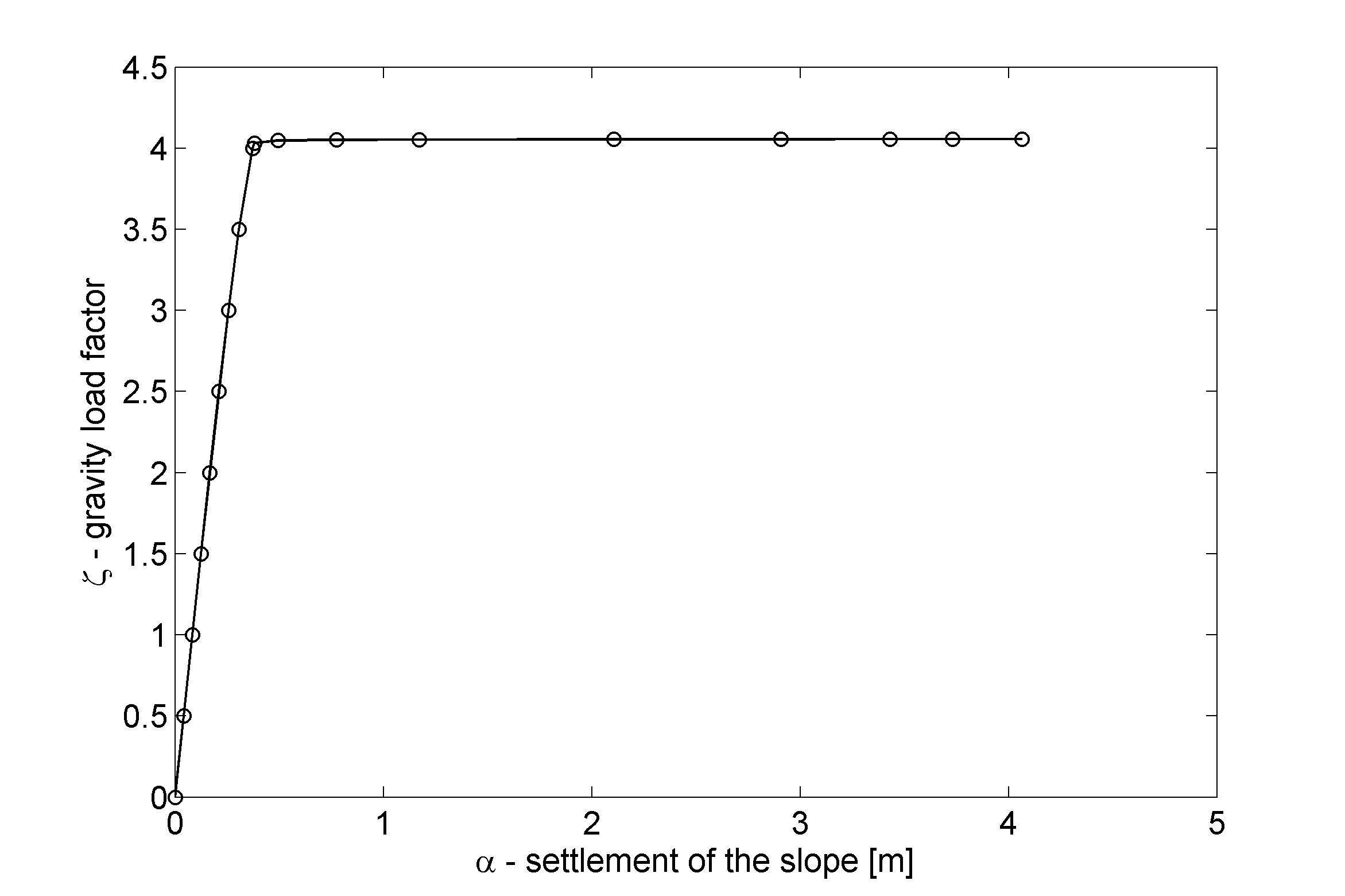
Figure 2: Load path for the direct method.

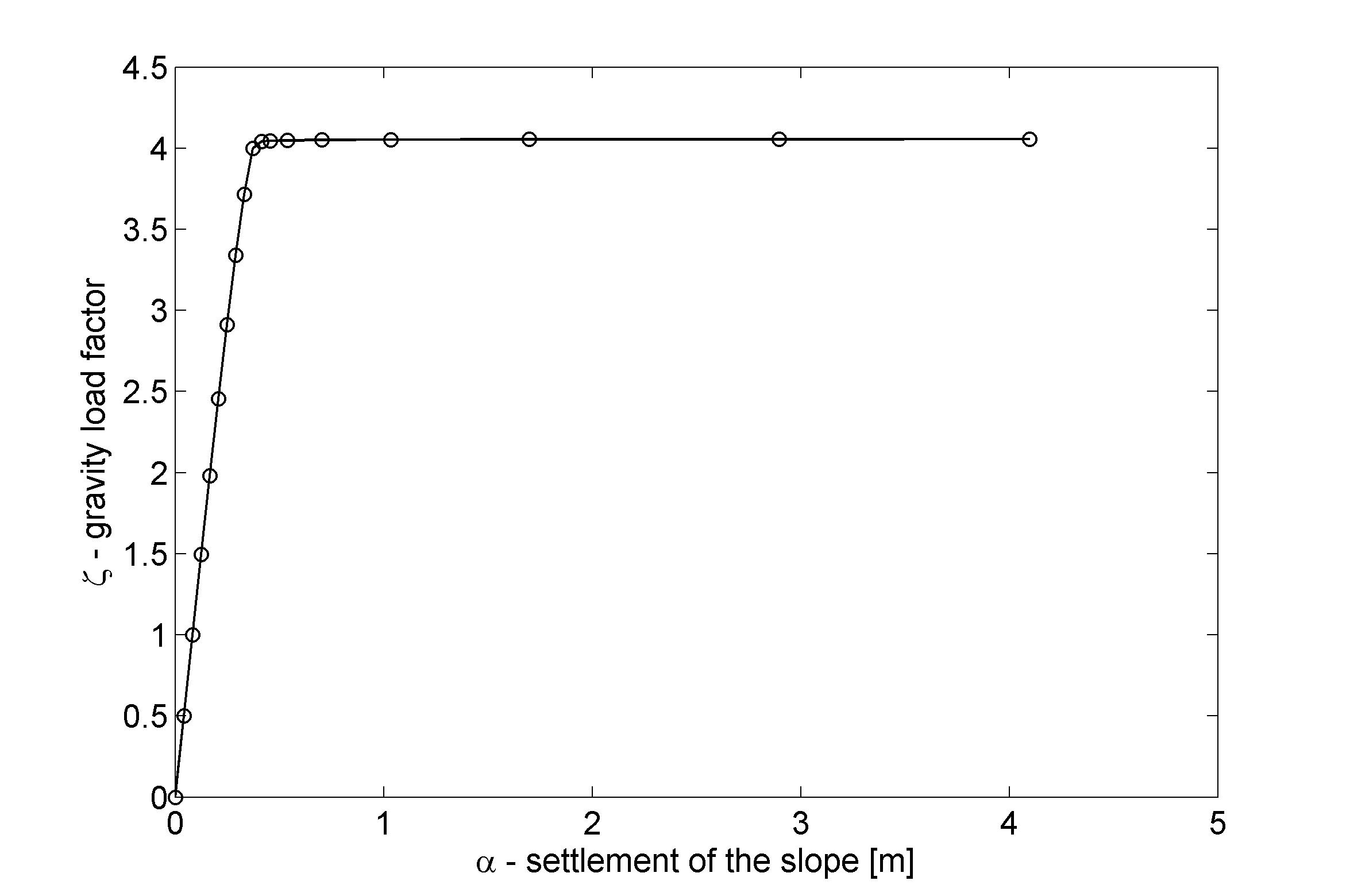
Figure 3: Load path for the indirect method.

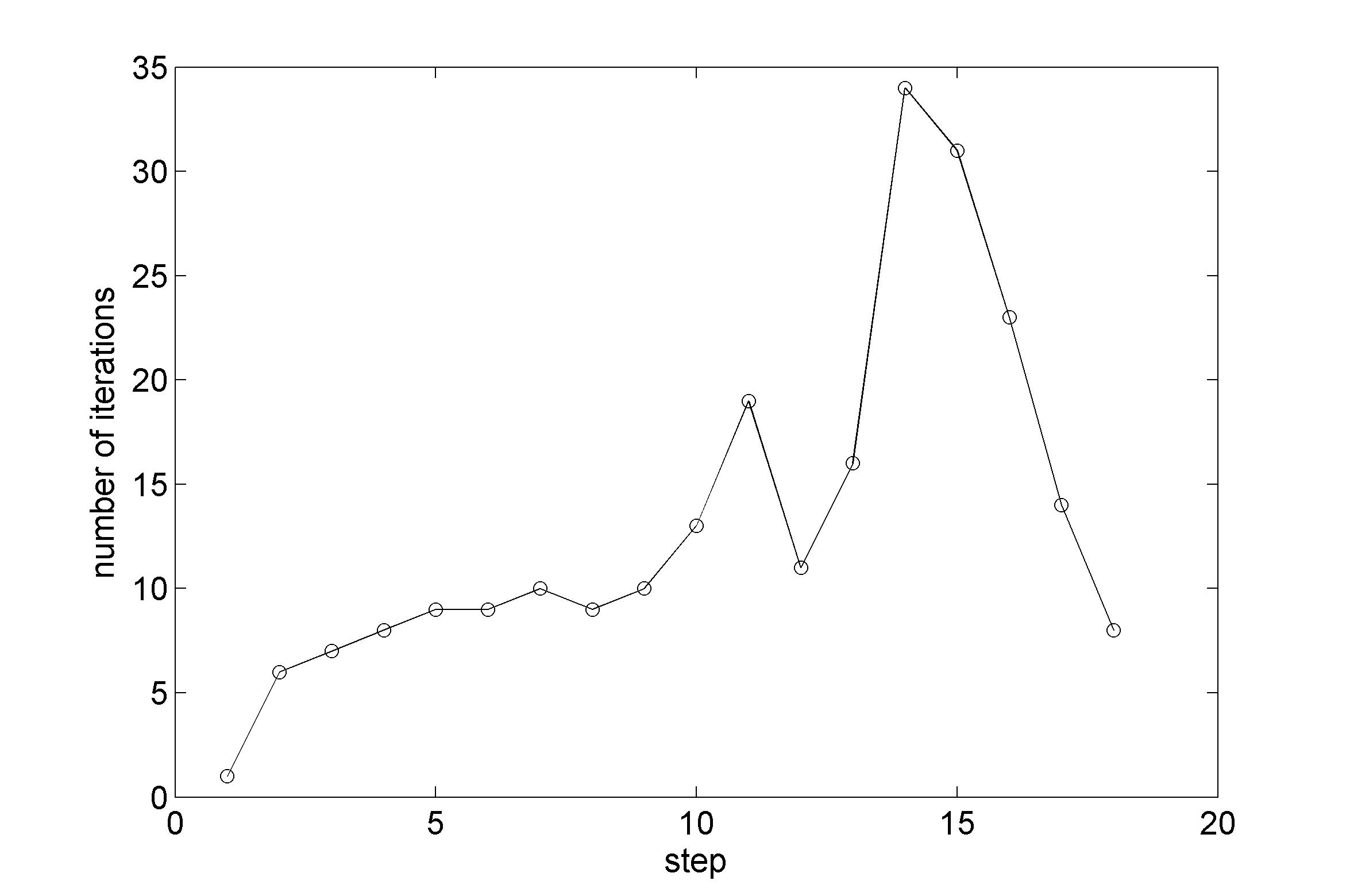
Figure 4: Number of iterations for ALG-$\zeta$.

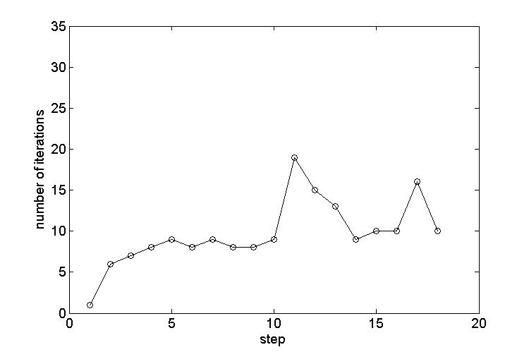
Figure 5: Number of iterations for ALG-$\alpha$.

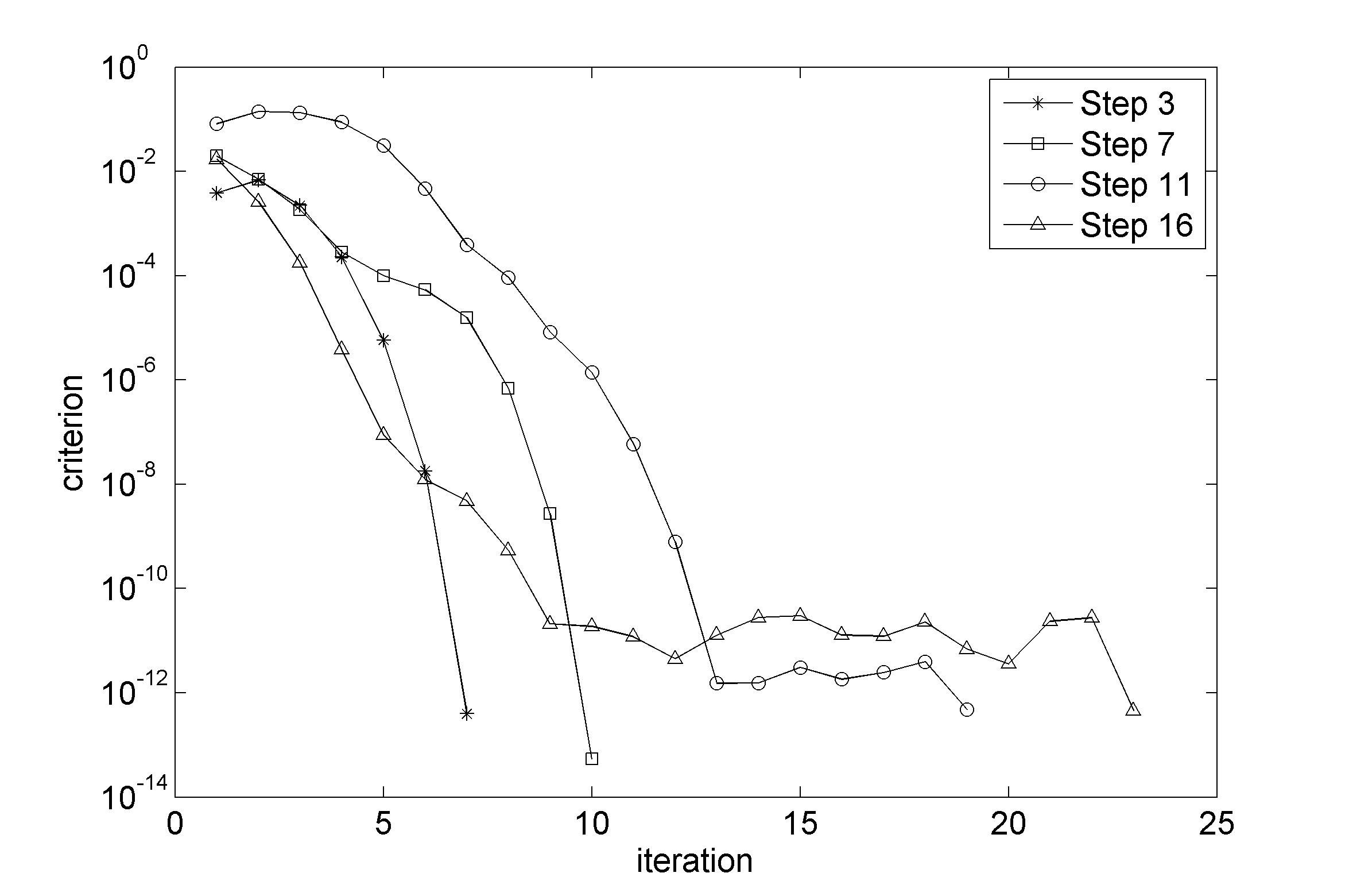
Figure 6: Convergence at selected steps for the direct method.

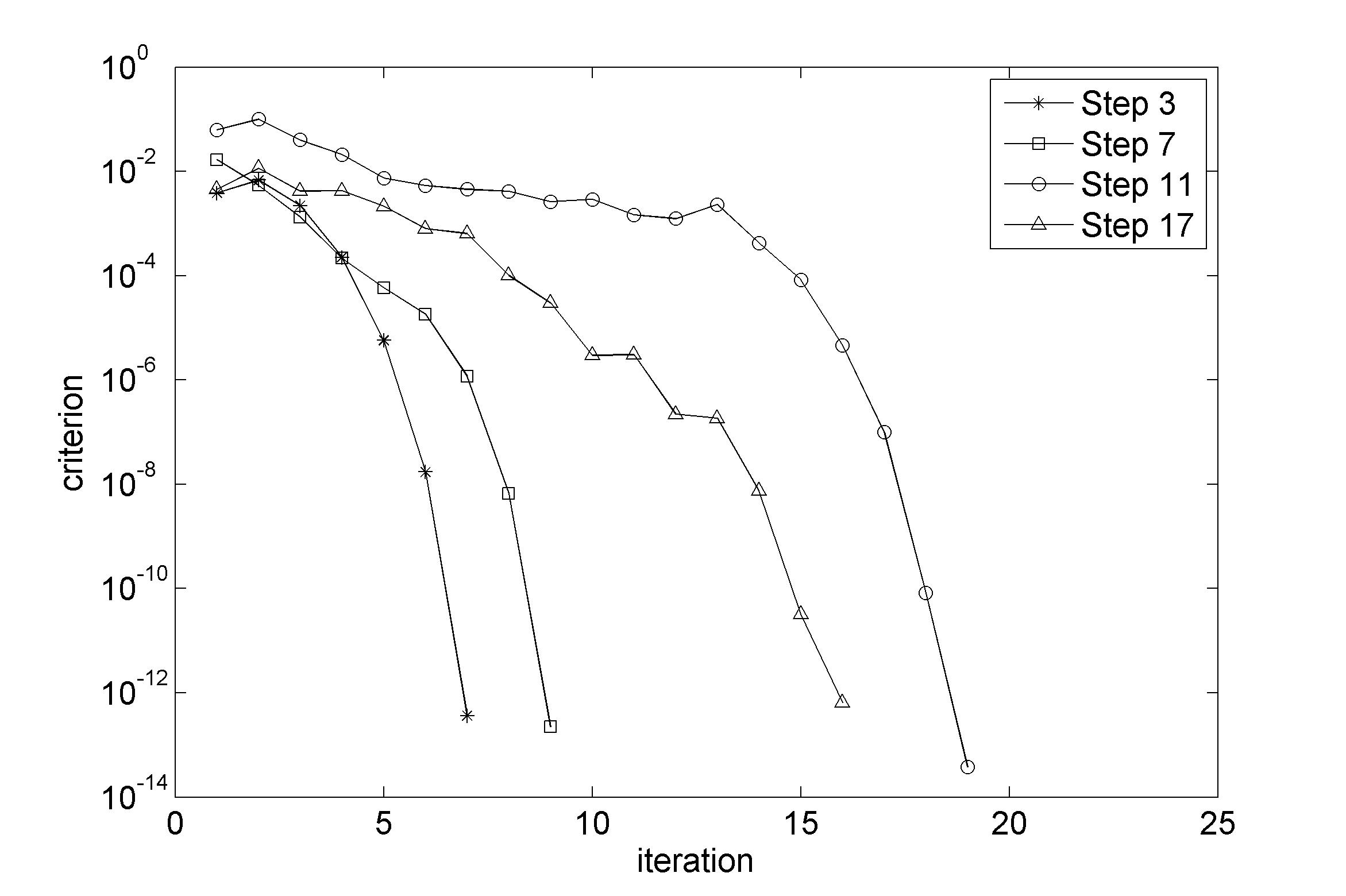
Figure 7: Convergence at selected steps for the indirect method.

The comparison of the direct and indirect methods is depicted in Figures 3-7. The resulting loading paths practically coincide for both methods and they are in accordance with [2, 1, 28]. The computed limit value is equal to 4.057 which is close to the estimate 4.045 known from [24]. Both methods need 18 load step and have superlinear convergence in each step. Their convergence is similar up to step 11. However, other comparisons turn out that the indirect method behaves better than the direct one. First, the indirect method has less number of iterations between steps 12 and 18. Secondly, the direct method contained 8 additional load steps without successful convergence while the indirect one convergences in each step. The successful load steps for both methods are depicted by the circular points in Figures 3 and 3, respectively. We see that the positions of these points are more convenient in Figure 3 than in Figure 3 with respect to the curvature of the loading path. Thirdly, we see in Figure 7 that the convergence in steps 11 and 16 is superlinear only up to 1e-10. Then, values of the stopping criterion oscillate. This is also observed for a few other steps of the direct method (e.g., steps 14 and 15). For the indirect method, this is not observed at any step. Finally, the computational times of the direct and indirect methods on a current laptop were approximately 9 and 7 minutes, respectively.

7.2 Associative perfect plastic 3D problem

Within the 3D slope stability experiment (code SS-MC-NP-3D), we compare the loading paths for the Q1 and Q2 hexahedral elements with 8 and 20 nodes, respectively. We consider $2\times 2\times 2$ and $3\times 3\times 3$ noded integration quadratures for these element types, respectively. Two hexahedral meshes are prepared for this experiment. For the Q1 elements, the meshes contain 5103 and 37597 nodal points, 34560 and 276480 integration points, respectively. For the Q2 elements, the meshes contain 19581 and 147257 nodal points, 116640 and 933120 integration points, respectively. We use the direct method of the incremental limit analysis which is terminated when the computed settlement exceeds 5 meters.

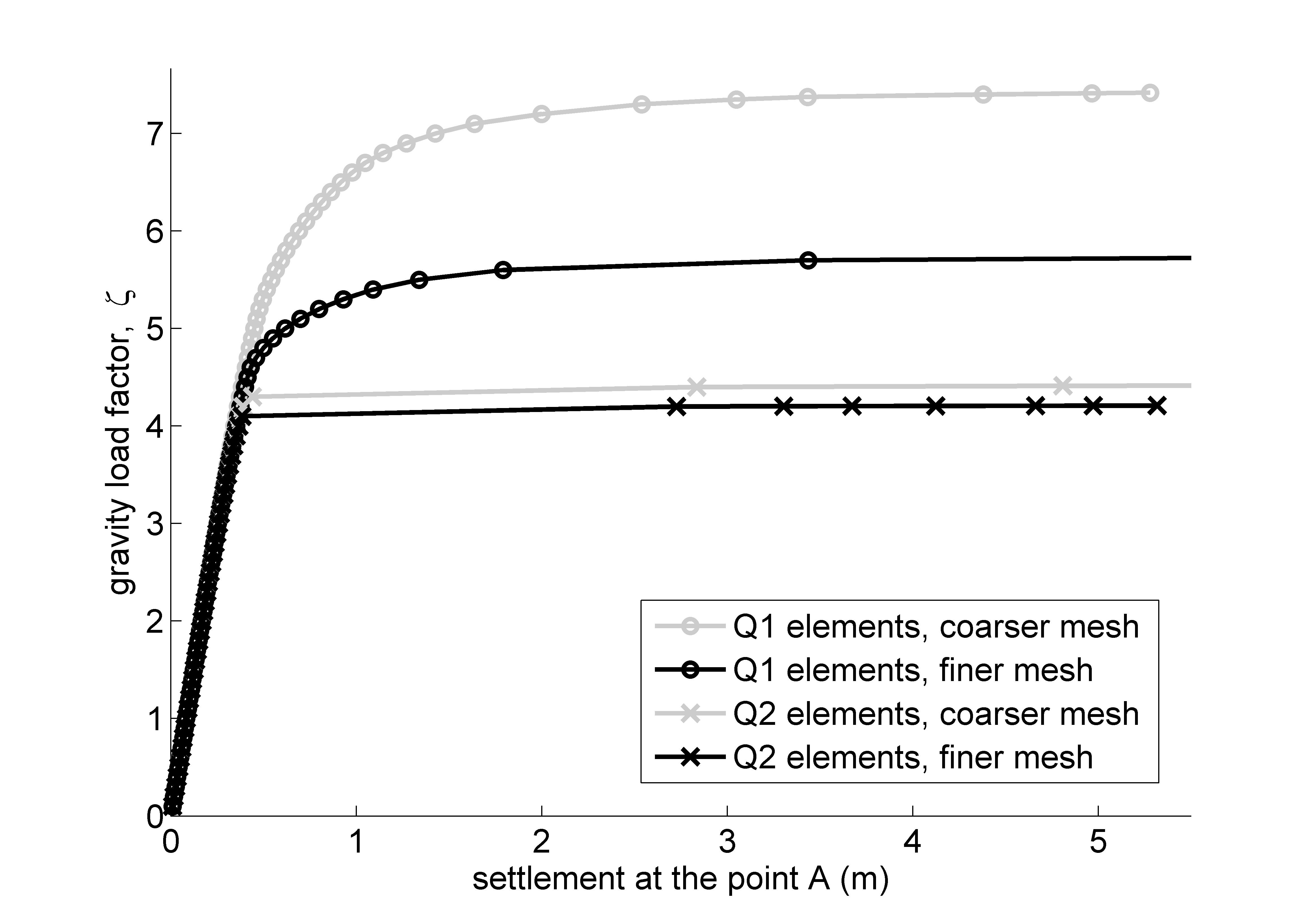
Figure 8: Comparison of the loading paths for $Q1$ and $Q2$ elements.

The corresponding loading paths are depicted in Figure 8. We observe that the estimated limit values of $\zeta$ are close to the expected value of 4.045 for the $Q2$ elements but not for the $Q1$ elements. To estimate $\zeta_{lim}$ using the $Q1$ elements, it would be necessary to use much finer meshes. Figures 10 and 10 illustrate failure at the end of the loading process for the Q2 elements and the finer mesh.

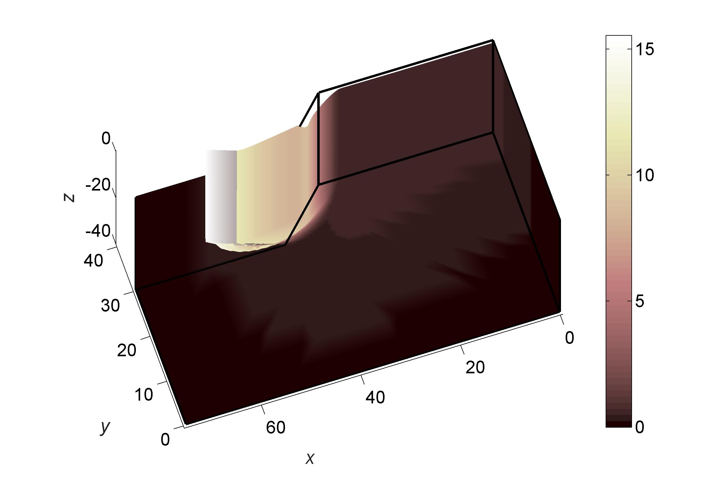
Figure 9: Total displacement and deformed shape at the end of the loading process.

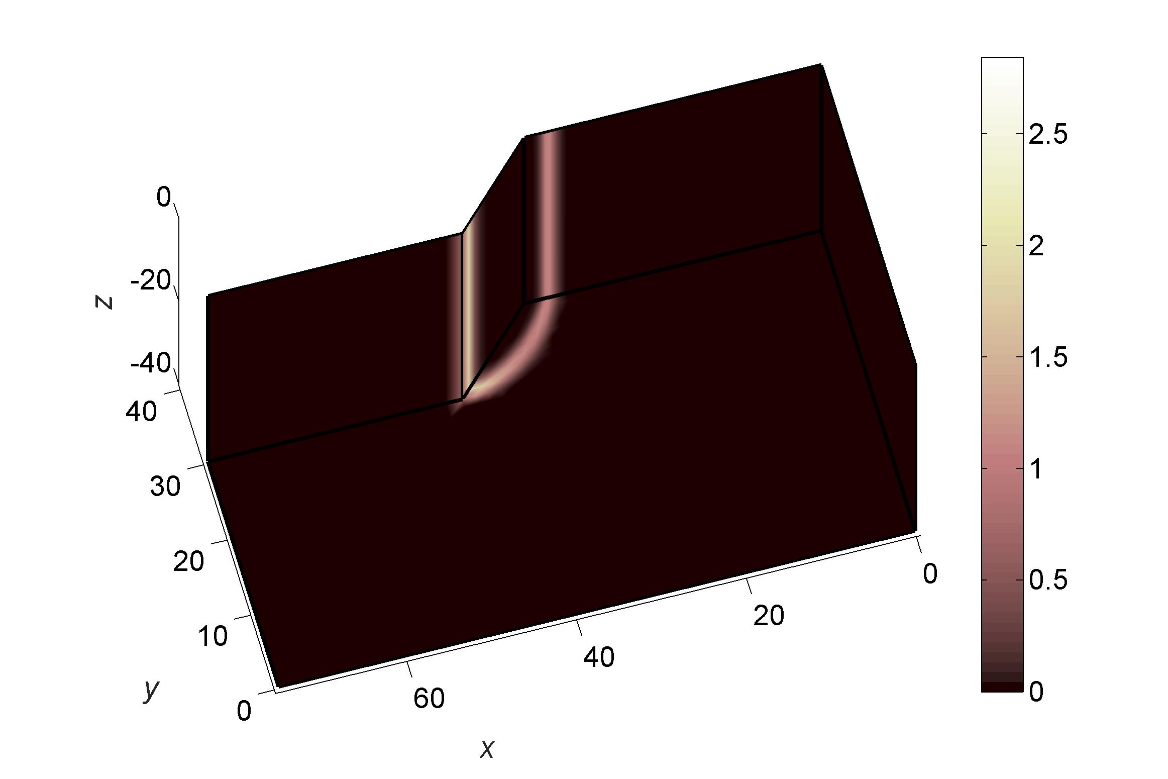
Figure 10: Plastic multipliers at the end of the loading process.

8 Conclusion

This paper extended the subdifferential-based constitutive solution technique proposed in [1] to elastoplastic models containing the Mohr-Coulomb yield criterion. It enabled deeper analysis of the constitutive problem discretized by the implicit Euler method and consequently led to several improvements within solution schemes. For example, a priori decision criteria characterizing each type of the return-mapping were derived even if the solution could not be found in closed form. The construction of the consistent tangent operator was also simplified. Moreover, the paper brought self-contained derivation of the constitutive operators which is not too often in Mohr-Coulomb plasticity.

The improved constitutive solution schemes were implemented within slope stability problems in 2D and 3D. To this end, the direct and also the indirect methods of the incremental limit analysis were used and combined with the semismooth Newton method. Local superlinear convergence in each step of both methods was observed. Further, it was illustrated that the indirect method led to more stable control of the loading process or that higher order finite elements reduced strong dependence on mesh.

Appendix

A. Simplified constitutive handling for the plane strain problem

The results of Section 4 and 5 are, of course, valid also for the plane strain problem. Nevertheless, in this case, one can simplify the forms of eigenprojections and their derivatives since we work only on the subspace $\mathbb{R}_{PS}$ of $\mathbb{R}^{3\times 3}_{sym}$ containing trial tensors in the form

$$\mbox{\boldmath$\eta$}=\left(\begin{array}[]{ccc}\eta_{11}&\eta_{12}&0\\ \eta_{12}&\eta_{22}&0\\ 0&0&\eta_{33}\end{array}\right).$$

To distinguish the derivatives of functions defined in $\mathbb{R}_{PS}$, we use the symbol $\tilde{\mathcal{D}}$ instead of $\mathcal{D}$. Define the functions

$$\tilde{\omega}_{1}(\mbox{\boldmath$\eta$}) := \frac{1}{2}\left[\eta_{11}+\eta_{22}+\sqrt{(\eta_{11}-\eta_{22})^{2}+4\eta_{12}^{2}}\right],$$

$$\tilde{\omega}_{2}(\mbox{\boldmath$\eta$}) := \frac{1}{2}\left[\eta_{11}+\eta_{22}-\sqrt{(\eta_{11}-\eta_{22})^{2}+4\eta_{12}^{2}}\right],$$

$$\tilde{\omega}_{3}(\mbox{\boldmath$\eta$}) := \eta_{33}$$

in $\mathbb{R}_{PS}$. Then $\tilde{\eta}_{i}=\tilde{\omega}_{i}(\mbox{\boldmath$\eta$})$, $i=1,2,3$, are the eigenvalues of $\eta$. These values are not ordered in general. We only know that $\tilde{\eta}_{1}\geq\tilde{\eta}_{2}$. Further, define

$$\tilde{\mbox{\boldmath$\eta$}}(\mbox{\boldmath$\eta$}):=\left(\begin{array}[]{r r r}\eta_{11}&\eta_{12}&0\\ \eta_{12}&\eta_{22}&0\\ 0&0&0\end{array}\right),\quad\tilde{\mbox{\boldmath$I$}}:=\left(\begin{array}[]{r r r}1&0&0\\ 0&1&0\\ 0&0&0\end{array}\right),\quad\tilde{\mbox{\boldmath$E$}}_{3}(\mbox{\boldmath$\eta$}):=\left(\begin{array}[]{r r r}0&0&0\\ 0&0&0\\ 0&0&1\end{array}\right),$$

$$\tilde{\mbox{\boldmath$E$}}_{1}(\mbox{\boldmath$\eta$}):=\left\{\begin{array}[]{c l}\frac{\tilde{\mbox{\boldmath$\eta$}}-\tilde{\eta}_{2}\tilde{\mbox{\boldmath$I$}}}{\tilde{\eta}_{1}-\tilde{\eta}_{2}},&\tilde{\eta}_{1}>\tilde{\eta}_{2}\\[5.69054pt] \tilde{\mbox{\boldmath$I$}},&\tilde{\eta}_{1}=\tilde{\eta}_{2}\end{array}\right.,\quad\tilde{\mbox{\boldmath$E$}}_{2}(\mbox{\boldmath$\eta$}):=\tilde{\mbox{\boldmath$I$}}-\tilde{\mbox{\boldmath$E$}}_{1}(\mbox{\boldmath$\eta$})$$

and

$$\tilde{\mathbb{E}}_{1}(\mbox{\boldmath$\eta$}):=\left\{\begin{array}[]{c l}\frac{1}{\tilde{\eta}_{1}-\tilde{\eta}_{2}}[\tilde{\mathbb{I}}-\tilde{\mbox{\boldmath$E$}}_{1}\otimes\tilde{\mbox{\boldmath$E$}}_{1}-\tilde{\mbox{\boldmath$E$}}_{2}\otimes\tilde{\mbox{\boldmath$E$}}_{2}],&\tilde{\eta}_{1}>\tilde{\eta}_{2}\\[5.69054pt] \mathbb{O},&\tilde{\eta}_{1}=\tilde{\eta}_{2}\end{array}\right.,\quad\tilde{\mathbb{E}}_{2}(\mbox{\boldmath$\eta$}):=-\tilde{\mathbb{E}}_{1}(\mbox{\boldmath$\eta$}),\quad\tilde{\mathbb{E}}_{3}(\mbox{\boldmath$\eta$}):=\mathbb{O},$$

where $\mathbb{O}$ denotes the zeroth fourth order tensor and $[\tilde{\mathbb{I}}]_{ijkl}=\delta_{ik}\delta_{jl}$, $i,j,k,l=1,2$, otherwise $[\tilde{\mathbb{I}}]_{ijkl}=0$. Clearly, $\mathcal{D}\tilde{\omega}_{3}(\mbox{\boldmath$\eta$})=\tilde{\mathcal{D}}\tilde{\omega}_{3}(\mbox{\boldmath$\eta$})=\tilde{\mbox{\boldmath$E$}}_{3}(\mbox{\boldmath$\eta$})$. If $\tilde{\eta}_{1}>\tilde{\eta}_{2}$ then

$$\tilde{\mbox{\boldmath$E$}}_{i}(\mbox{\boldmath$\eta$})=\tilde{\mathcal{D}}\tilde{\omega}_{i}(\mbox{\boldmath$\eta$}),\quad\tilde{\mathbb{E}}_{i}(\mbox{\boldmath$\eta$})=\tilde{\mathcal{D}}\tilde{\mbox{\boldmath$E$}}_{i}(\mbox{\boldmath$\eta$})\qquad\mbox{in }\mathbb{R}_{PS},\quad i=1,2.$$

It is worth mentioning that these formulas need not hold in $\mathbb{R}^{3\times 3}_{sym}$ in general. Similar formulas are also introduced in [2, Appendix A].

Now, it is necessary to reorder the eigenvalues of $\mbox{\boldmath$\eta$}\in\mathbb{R}_{PS}$. Denote the ordered eigenvalues as $\eta_{1},\eta_{2},\eta_{3}$, i.e., $\eta_{1}:=\max\{\tilde{\eta}_{1},\tilde{\eta}_{3}\}$ and $\eta_{3}:=\min\{\tilde{\eta}_{2},\tilde{\eta}_{3}\}$. Consequently, we reorder the functions $\tilde{\omega}_{i}$, $\tilde{\mbox{\boldmath$E$}}_{i}$, $\tilde{\mathbb{E}}_{i}$, $i=1,2,3$, leading to the functions $\omega_{i}$, $\mbox{\boldmath$E$}_{i}$, $\mathbb{E}_{i}$, $i=1,2,3$. To complete the notation, one can easily set

$$\mbox{\boldmath$E$}_{12}(\mbox{\boldmath$\eta$}):=\mbox{\boldmath$E$}_{1}(\mbox{\boldmath$\eta$})+\mbox{\boldmath$E$}_{2}(\mbox{\boldmath$\eta$}),\quad\mbox{\boldmath$E$}_{23}(\mbox{\boldmath$\eta$}):=\mbox{\boldmath$E$}_{2}(\mbox{\boldmath$\eta$})+\mbox{\boldmath$E$}_{3}(\mbox{\boldmath$\eta$})\quad\forall\mbox{\boldmath$\eta$}\in\mathbb{R}_{PS}.$$

Finally, one can straightforwardly use the functions $\omega_{i}$, $\mbox{\boldmath$E$}_{i}$, $\mathbb{E}_{i}$, $i=1,2,3$, $\mbox{\boldmath$E$}_{12}$ and $\mbox{\boldmath$E$}_{23}$ within Section 5 when the plane strain assumptions are considered.

B. Algebraic representation of second and fourth order tensors

Within our implementation, we use the standard algebraic representation of stress and strain second order tensors specified below but a little bit different representation of fourth order tensors in comparison to [2, Appendix D]. We assume that a fourth order tensor $\mathbb{C}$ represents a linear mapping from $\mathbb{R}^{3\times 3}_{sym}$ into $\mathbb{R}^{3\times 3}_{sym}$. Therefore, the components $[\mathbb{C}]_{ijkl}\equiv C_{ijkl}$ of $\mathbb{C}$ satisfy

$$\sum_{k,l}C_{ijkl}\eta_{kl}=\sum_{k,l}C_{jikl}\eta_{kl}\quad\forall\mbox{\boldmath$\eta$}\in\mathbb{R}^{3\times 3}_{sym},\;\;\eta_{kl}=[\mbox{\boldmath$\eta$}]_{kl}.$$

The choice $\eta_{kl}=\delta_{mk}\delta_{nl}+\delta_{nk}\delta_{ml}$ implies that $\mbox{\boldmath$\eta$}\in\mathbb{R}^{3\times 3}_{sym}$ for any $m,n=1,2,3$ and

$$C_{ijmn}+C_{ijnm}=C_{jimn}+C_{jinm}\quad\forall i,j,m,n=1,2,3.$$ (B.1)

Notice that in [2, Appendix D], the stronger assumptions on the components are required: $C_{ijmn}=C_{ijnm}=C_{jimn}=C_{jinm}$.

We distinguish two cases: the 3D problem and its plane strain reduction.

The 3D problem

Let $\mbox{\boldmath$\tau$},\mbox{\boldmath$\eta$}\in\mathbb{R}^{3\times 3}_{sym}$ denote stress and strain tensors, respectively. Then they are represented by vectors $\mathbf{t}=(\tau_{11},\tau_{22},\tau_{33},\tau_{12},\tau_{23},\tau_{13})^{T}$ and $\mathbf{n}=(\eta_{11},\eta_{22},\eta_{33},2\eta_{12},2\eta_{23},2\eta_{13})^{T}$ where $\tau_{ij}$ and $\eta_{ij}$ are the components of $\tau$, and $\eta$, respectively. Clearly, $\mbox{\boldmath$\tau$}:\mbox{\boldmath$\eta$}=\mathbf{t}\cdot\mathbf{n}$. A fourth order tensor $\mathbb{C}$ is represented by matrix $\mbox{\boldmath$C$}\in\mathbb{R}^{6\times 6}$. Since fourth order tensors are applied on strain tensors within the implementation, we require that

$$\mbox{\boldmath$\eta$}:\mathbb{C}:\mbox{\boldmath$\varepsilon$}=\mathbf{n}\cdot\mbox{\boldmath$C$}\mathbf{e}$$ (B.2)

holds for any strain tensors $\eta$ and $\varepsilon$. Here, $\mathbf{n}$ and $\mathbf{e}$ denote the algebraic counterparts of $\eta$ and $\varepsilon$, respectively. From (B.1) and (B.2), one can derive that

$$\mbox{\boldmath$C$}=\left(\begin{array}[]{c c c c c c}C_{1111}&C_{1122}&C_{1133}&\frac{1}{2}[C_{1112}+C_{1121}]&\frac{1}{2}[C_{1123}+C_{1132}]&\frac{1}{2}[C_{1113}+C_{1131}]\\[2.84526pt] C_{2211}&C_{2222}&C_{2233}&\frac{1}{2}[C_{2212}+C_{2221}]&\frac{1}{2}[C_{2223}+C_{2232}]&\frac{1}{2}[C_{2213}+C_{2231}]\\[2.84526pt] C_{3311}&C_{3322}&C_{3333}&\frac{1}{2}[C_{3312}+C_{3321}]&\frac{1}{2}[C_{3323}+C_{3332}]&\frac{1}{2}[C_{3313}+C_{3331}]\\[2.84526pt] C_{1211}&C_{1222}&C_{1233}&\frac{1}{2}[C_{1212}+C_{1221}]&\frac{1}{2}[C_{1223}+C_{1232}]&\frac{1}{2}[C_{1213}+C_{1231}]\\[2.84526pt] C_{2311}&C_{2322}&C_{2333}&\frac{1}{2}[C_{2312}+C_{2321}]&\frac{1}{2}[C_{2323}+C_{2332}]&\frac{1}{2}[C_{2313}+C_{2331}]\\[2.84526pt] C_{1311}&C_{1322}&C_{1333}&\frac{1}{2}[C_{1312}+C_{1321}]&\frac{1}{2}[C_{1323}+C_{1332}]&\frac{1}{2}[C_{1313}+C_{1331}]\end{array}\right).$$

Indeed, the choices $\varepsilon_{kl}=\frac{1}{2}(\delta_{2k}\delta_{3l}+\delta_{2k}\delta_{3l})$, $\eta_{ij}=\frac{1}{2}(\delta_{1i}\delta_{2j}+\delta_{2i}\delta_{1j})$ imply $\mathbf{e}=(0,0,0,0,1,0)^{T}$ and $\mathbf{n}=(0,0,0,1,0,0)^{T}$. Hence,

$$[\mbox{\boldmath$C$}]_{45}=\mathbf{n}\cdot\mbox{\boldmath$C$}\mathbf{e}\stackrel{{\scriptstyle(\ref{C_algebra})}}{{=}}\eta:\mathbb{C}:\varepsilon=\frac{1}{4}[C_{1223}+C_{1232}+C_{2123}+C_{2132}]\stackrel{{\scriptstyle(\ref{C_sym})}}{{=}}\frac{1}{2}[C_{1223}+C_{1232}].$$

Similarly, one can derive the forms of other components of $C$. Notice that the algebraic representation of $\mathbb{C}$ is more general than in [2, Appendix D].

We introduce three examples useful for the Mohr-Coulomb model:

1. Let $\mathbb{C}=\mathbb{I}$. Then $C_{ijkl}=\delta_{ik}\delta_{jl}$ and $\mbox{\boldmath$C$}=\mbox{diag}(1,1,1,1/2,1/2,1/2)$. Notice that the same matrix is derived in [2, Appendix D] although the tensor $\mathbb{I}_{S}$, $[\mathbb{I}_{S}]_{ijkl}=\frac{1}{2}(\delta_{ik}\delta_{jl}+\delta_{il}\delta_{jk})$, is used there instead of $\mathbb{I}$.

2. Let $\mathbb{C}=\mbox{\boldmath$\tau$}\otimes\mbox{\boldmath$\sigma$}$ where $\mbox{\boldmath$\sigma$},\mbox{\boldmath$\tau$}$ are arbitrary chosen stress tensors. Denote $\mathbf{s}$ and $\mathbf{t}$ as the algebraic counterparts to $\mbox{\boldmath$\sigma$},\mbox{\boldmath$\tau$}$, respectively. Then $\mbox{\boldmath$C$}=\mathbf{s}\mathbf{t}^{T}$.

3. Let $\mathbb{C}=\mathcal{D}(\mbox{\boldmath$\eta$}^{2})$. Then $C_{ijkl}=\delta_{ik}\eta_{lj}+\delta_{jl}\eta_{ik}$ and

   $$\mbox{\boldmath$C$}=\left(\begin{array}[]{c c c c c c}2\eta_{11}&0&0&\eta_{12}&0&\eta_{13}\\[2.84526pt] 0&2\eta_{22}&0&\eta_{12}&\eta_{23}&0\\[2.84526pt] 0&0&2\eta_{33}&0&\eta_{23}&\eta_{13}\\[2.84526pt] \eta_{12}&\eta_{12}&0&\frac{1}{2}[\eta_{11}+\eta_{22}]&\frac{1}{2}\eta_{13}&\frac{1}{2}\eta_{23}\\[2.84526pt] 0&\eta_{23}&\eta_{23}&\frac{1}{2}\eta_{13}&\frac{1}{2}[\eta_{22}+\eta_{33}]&\frac{1}{2}\eta_{12}\\[2.84526pt] \eta_{13}&0&\eta_{13}&\frac{1}{2}\eta_{23}&\frac{1}{2}\eta_{12}&\frac{1}{2}[\eta_{11}+\eta_{33}]\end{array}\right).$$

The plane strain problem

Let $\tau$ and $\eta$ denote stress and strain second order tensors, respectively. Then they are represented by the vectors $\mathbf{t}=(\tau_{11},\tau_{22},\tau_{12},\tau_{33})^{T}$ and $\mathbf{n}=(\eta_{11},\eta_{22},2\eta_{12},\eta_{33})^{T}$ where $\tau_{ij}$ and $\eta_{ij}$ are components of $\tau$, and $\eta$, respectively. Clearly, $\mbox{\boldmath$\tau$}:\mbox{\boldmath$\eta$}=\mathbf{t}\cdot\mathbf{n}$. Notice that the component $\eta_{33}$ vanishes for the strain tensor but not for the plastic strain tensor.

The fourth order tensor $\mathbb{C}$ can be represented by matrix $\mbox{\boldmath$C$}\in\mathbb{R}^{4\times 4}$. Similarly as for the 3D problem, one can derive that

$$\mbox{\boldmath$C$}=\left(\begin{array}[]{c c c c}C_{1111}&C_{1122}&\frac{1}{2}[C_{1112}+C_{1121}]&C_{1133}\\[2.84526pt] C_{2211}&C_{2222}&\frac{1}{2}[C_{2212}+C_{2221}]&C_{2233}\\[2.84526pt] C_{1211}&C_{1222}&\frac{1}{2}[C_{1212}+C_{1221}]&C_{1233}\\[2.84526pt] C_{3311}&C_{3322}&\frac{1}{2}[C_{3312}+C_{3321}]&C_{3333}\end{array}\right).$$

Finally, it is worth mentioning that for assembling the tangent stiffness matrix, it is sufficient to save only the components $(\mbox{\boldmath$C$})_{ij}$ where $i,j=1,2,3$.

References

- [1] Sysala S, Cermak M, Koudelka T, Kruis J, Zeman J, Blaheta R. Subdifferential-based implicit return-mapping operators in computational plasticity. ZAMM-Journal of Applied Mathematics and Mechanics/Zeitschrift für Angewandte Mathematik und Mechanik 2016; .
- [2] de Souza Neto EA, Perić D, Owen DRJ. Computational Methods for Plasticity. Wiley-Blackwell, 2008.
- [3] Clausen J, Damkilde L, Andersen LV. Robust and efficient handling of yield surface discontinuities in elasto-plastic finite element calculations. Engineering Computations 2015; 32(6):1722–1752.
- [4] Lin C, Li YM. A return mapping algorithm for unified strength theory model. International Journal for Numerical Methods in Engineering 2015; 104(8):749–766.
- [5] Larsson R, Runesson K. Implicit integration and consistent linearization for yield criteria of the mohr–coulomb type. Mechanics of Cohesive-frictional Materials 1996; 1(4):367–383.
- [6] Borja RI, Sama KM, Sanz PF. On the numerical integration of three-invariant elastoplastic constitutive models. Computer Methods in Applied Mechanics and Engineering 2003; 192(9-10):1227–1258.
- [7] Karaoulanis FE. Implicit numerical integration of nonsmooth multisurface yield criteria in the principal stress space. Arch Computat Methods Eng 2013; 20(3):263–308.
- [8] Koiter WT. Stress-strain relations, uniqueness and variational theorems for elastic-plastic materials with a singular yield surface. Quarterly of Applied Mathematics 1953; 11(3):350–354.
- [9] de Borst R. Integration of plasticity equations for singular yield functions. Computers & Structures 1987; 26(5):823–829.
- [10] Han W, Reddy BD. Plasticity: mathematical theory and numerical analysis. Springer-Verlag, 1999.
- [11] Berga A. Mathematical and numerical modeling of the non-associated plasticity of soils—part 1: The boundary value problem. International Journal of Non-Linear Mechanics 2012; 47(1):26–35.
- [12] Simo JC, Hughes TJ. Computational inelasticity. Springer Science & Business Media, 2006.
- [13] Starman B, Halilovič M, Vrh M, Štok B. Consistent tangent operator for cutting-plane algorithm of elasto-plasticity. Computer Methods in Applied Mechanics and Engineering 2014; 272:214–232.
- [14] Clausen J, Damkilde L, Andersen L. Efficient return algorithms for associated plasticity with multiple yield planes. International Journal for Numerical Methods in Engineering 2006; 66(6):1036–1059.
- [15] Abbo A, Lyamin A, Sloan S, Hambleton J. A C2 continuous approximation to the Mohr–Coulomb yield surface. International Journal of Solids and Structures 2011; 48(21):3001–3010.
- [16] Borja RI. Plasticity. Springer, 2013.
- [17] Čermák M, Kozubek T, Sysala S, Valdman J. A TFETI domain decomposition solver for elastoplastic problems. Applied Mathematics and Computation 2014; 231:634–653.
- [18] Gruber PG, Valdman J. Solution of one-time-step problems in elastoplasticity by a slant Newton method. SIAM J. Sci. Comput. 2009; 31(2):1558–1580.
- [19] Sauter M, Wieners C. On the superlinear convergence in computational elasto-plasticity. Computer Methods in Applied Mechanics and Engineering 2011; 200(49-52):3646–3658.
- [20] Sysala S. Application of a modified semismooth Newton method to some elasto-plastic problems. Mathematics and Computers in Simulation 2012; 82(10):2004–2021.
- [21] Sysala S. Properties and simplifications of constitutive time-discretized elastoplastic operators. ZAMM - Journal of Applied Mathematics and Mechanics / Zeitschrift für Angewandte Mathematik und Mechanik 2014; 94(3):233–255.
- [22] Carlson DE, Hoger A. The derivative of a tensor-valued function of a tensor. The Quarterly of Applied Mathematics 1986; 44:409–423.
- [23] de Borst R, Crisfield MA, Remmers JJC, Verhoosel CV. Non-Linear Finite Element Analysis of Solids and Structures. Wiley-Blackwell, 2012.
- [24] Chen WF, Liu X. Limit analysis in soil mechanics. Elsevier, 2012.
- [25] Sysala S, Haslinger J, Hlaváček I, Cermak M. Discretization and numerical realization of contact problems for elastic-perfectly plastic bodies. PART I - discretization, limit analysis. ZAMM-Journal of Applied Mathematics and Mechanics/Zeitschrift für Angewandte Mathematik und Mechanik 2015; 95(4):333–353.
- [26] Cermak M, Haslinger J, Kozubek T, Sysala S. Discretization and numerical realization of contact problems for elastic-perfectly plastic bodies. PART II - numerical realization, limit analysis. ZAMM - Journal of Applied Mathematics and Mechanics / Zeitschrift für Angewandte Mathematik und Mechanik 2015; 95(12):1348–1371.
- [27] Haslinger J, Repin S, Sysala S. A reliable incremental method of computing the limit load in deformation plasticity based on compliance: Continuous and discrete setting. Journal of Computational and Applied Mathematics 2016; 303:156–170.
- [28] Haslinger J, Repin S, Sysala S. Guaranteed and computable bounds of the limit load for variational problems with linear growth energy functionals. Applications of Mathematics 2016; 61(5):527–564.
- [29] Ruszczyński AP. Nonlinear optimization. Princeton university press, 2006.
- [30] Sysala S, Cermak M. Experimental matlab code for the slope stability benchmark – SS-MC-NP-3D, SS-MC-NH, SS-MC-NP-Acontrol 2016. URL www.ugn.cas.cz/?p=publish/output.php, (or www.ugn.cas.cz - Publications - Other outputs - SS-MC-NP-3D, SS-MC-NH, SS-MC-NP-Acontrol).