High-resolution Observations of a Flux Rope with the Interface Region Imaging Spectrograph

Abstract

We report the observations of a flux rope at transition region temperatures with the Interface Region Imaging Spectrograph (IRIS) on 30 August 2014. Initially, magnetic flux cancellation constantly took place and a filament was activated. Then the bright material from the filament moved southward and tracked out several fine structures. These fine structures were twisted and tangled with each other, and appeared as a small flux rope at 1330 Å, with a total twist of about 4$\pi$. Afterwards, the flux rope underwent a counter-clockwise (viewed top-down) unwinding motion around its axis. Spectral observations of C ii 1335.71 Å at the southern leg of the flux rope showed that Doppler redshifts of 6$-$24 km s^-1 appeared at the western side of the axis, which is consistent with the counter-clockwise rotation motion. We suggest that the magnetic flux cancellation initiates reconnection and some activation of the flux rope. The stored twist and magnetic helicity of the flux rope are transported into the upper atmosphere by the unwinding motion in the late stage. The small-scale flux rope (width of 8.3^′′) had a cylindrical shape with helical field lines, similar to the morphology of the large-scale CME core (width of 1.54 $R_{\odot}$) on 2 June 1998. This similarity shows the presence of flux ropes of different scales on the Sun.

1 Introduction

Eruptive solar filaments and coronal mass ejections (CMEs) often exhibit a clear helical geometry (about 40% for CMEs; Vourlidas et al., 2012), indicating the eruption of a magnetic flux rope. A magnetic flux rope becomes kink-unstable if the twist exceeds a critical value of 2.5$\pi$$-$3.5$\pi$ (Hood and Priest, 1981; Fan, 2005; Török and Kliem, 2005). Then the axis of the flux rope undergoes writhing motions, and the twist is transformed into the writhe of the axis, since the magnetic helicity is essentially conserved (Ji et al., 2003; Rust and LaBonte, 2005). The kink instability can initiate the rise motion of the flux rope and is considered as one type of mechanism that triggers the CME and associated activities (Török and Kliem, 2003; Liu et al., 2007; Yan et al., 2014).

However, a basic question about the formation of the flux rope is not well understood. Some theoretical models suggest that the flux rope is formed through magnetic reconnection, which converts sheared arcades into a helical structure (Pneuman, 1983; van Ballegooijen and Martens, 1989). Joshi et al. (2014a) showed an example of compound flux rope formation via merging of two different flux ropes, consistent with the tether cutting magnetic reconnection scenario (Moore et al., 2001). Cheng et al. (2014) suggested that magnetic reconnection was responsible for the formation of a double-decker magnetic flux rope. Another possibility is the emergence of the flux rope from below the photosphere into the corona. The helical structure is formed deep in the convection zone before its emergence (Rust and Kumar, 1994; Lites, 2005). Okamoto et al. (2008) analyzed the vector magnetic fields on the photosphere under a filament and concluded that a helical flux rope was emerging from below the photosphere.

Based on the nonlinear force-free field (NLFFF) extrapolation technique, Guo et al. (2010) and Canou and Amari (2010) showed the presence of twisted flux ropes and found that the location of the magnetic dips within the flux ropes agrees with the observed filament in H$\alpha$ images. Moreover, the formation and eruption of flux ropes have been simulated by many authors (Fan and Gibson, 2004; Amari et al., 2010). Aulanier et al. (2010) carried out the magnetohydrodynamic (MHD) simulation and found that the photospheric flux-cancellations in a bald-patch separatrix and tether-cutting coronal reconnection are key mechanisms for the formation of flux ropes.

Recently, the direct observations of flux ropes in the low corona have been reported (Li and Zhang, 2013a, 2013c, 2014; Chen et al., 2014a, 2014b; Song et al., 2014; Joshi et al., 2014b) by using the extreme ultraviolet (EUV) data from the Atmospheric Imaging Assembly (AIA; Lemen et al., 2012) onboard the Solar Dynamics Observatory (SDO; Pesnell et al., 2012). Kumar et al. (2010) presented a successive activation of magnetic flux ropes in chromospheric and EUV lines and concluded that such activation plays an important role in triggering the flare. Srivastava et al. (2010) reported the observations of a flux rope with a high twist angle of 12$\pi$ in the channels of Ca ii H (3968 Å) and 171 Å. The recently launched Interface Region Imaging Spectrograph (IRIS; De Pontieu et al., 2014) mission is now providing observations of the transition region (TR) and chromosphere with remarkable spatial and spectral resolution. The TR is the interface between the chromosphere and the corona, where the temperature rapidly rises from 25000 K to 1 MK. In this work, we present the observations of a flux rope at TR temperatures based on IRIS and SDO data.

2 Observations and Data Analysis

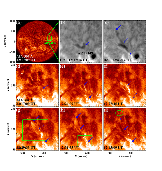
Figure 1.: SDO$/$AIA 304 Å and GONG H$\alpha$ images showing the evolution of the erupting filament on 30 August 2014 (a 304 Å movie is also available as electronic supplementary material). Blue arrows point to the analyzed filament. The green rectangle in panel (g) denotes the field of view (FOV) of Figures 3(a)-(b), and the green rectangle in panel (h) displays the FOV of the images in Figures 4 and 5. The green ellipse in panel (i) shows the counterclockwise rotation of the filament.Fig1

IRIS records spectra over three wavelength bands of the far ultraviolet (1332$-$1358 Å and 1389$-$1406 Å) and the near ultraviolet (2782$-$2834 Å), and also obtains slit-jaw images (SJIs) centered at 1330, 1400, 2796 and 2832 Å, with 0.33^′′$-$0.4^′′ spatial resolution (De Pontieu et al., 2014). For the analyzed event, the IRIS observation was taken from 11:12 UT to 17:13 UT on 30 August 2014. The SJIs are taken in the 1330 and 2796 Å channels. The 1330 Å channel best shows the flux rope and we focus on this channel in this study. The 1330 Å filter records emission coming from the C ii 1335.71 Å line and the UV continuum. The C ii 1335.71 Å line is formed in the lower TR and corresponds to a temperature of about 10^4.4 K (Tian et al., 2014; Li et al., 2014). The SJIs at 1330 Å have a cadence of $\approx$ 19 s and a sampling of 0.166^′′ pixel^-1. The spectral observations covering the strong emission line of C ii 1335.71 Å are analyzed in detail. The spectral data are taken in a sit-and-stare mode with 8 s exposure time and 9 s cadence. The present study uses IRIS level 2 data provided by the IRIS team. Dark current removal, flat-field and geometric correction have been taken into account in the level 2 data. The emission in the the IRIS spectral line of C ii is shifted along the IRIS slit, and this offset is achieved by checking the position of horizontal fiducial lines.

The SDO observations are also used here in order to analyze the filament evolution. The AIA takes full-disk images in 10 (E)UV channels at 1.5^′′ resolution and high cadence of 12 s. Among these channels, the high-cadence 171 and 304 Å observations are chosen. The 171 Å channel corresponds to a temperature of about 0.6 MK (Fe ix) and the channel of 304 Å (He ii) is at 0.05 MK (O’Dwyer et al., 2010). Moreover, we also use the full-disk line-of-sight (LOS) magnetic field data from the Helioseismic and Magnetic Imager (HMI; Scherrer et al., 2012) onboard SDO, with a cadence of $\approx$ 45 s and a sampling of 0.5^′′ pixel^-1. NSO$-$GONG H$\alpha$ data are used to investigate the chromospheric configuration of the filament. GONG collects H$\alpha$ data at seven sites around the world with a spatial resolution of 1.0^′′ pixel^-1 and a cadence of around 1 min (Harvey et al., 2011). The morphology of the flux rope reminds us of the CME event occurring on 2 June 1998. The Large Angle and Spectrometric Coronagraph (LASCO; Brueckner et al., 1995) experiment on board the Solar and Heliospheric Observatory (SOHO) records the CME with a “net-like cylinder” shape, similar to the flux rope observed by the IRIS.

3 Results

3.1 Failed Eruption of the Filament

The filament analyzed here is located in the north of NOAA active region (AR) 12149 near the coordinates (600^′′, 50^′′) around 12:20 UT on 30 August 2014 (Figure 1(a)). It has a length of about 50^′′, the typical length of a mini-filament (Zheng et al., 2012; Kumar and Cho, 2014). Before the activation, the filament appeared faint both in H$\alpha$ and EUV wavelengths (Figures 1(b) and (d)). At about 12:20 UT, the filament was activated and then it could be clearly observed at 304 Å. The associated EUV brightenings appeared at the west of the filament and increased until 12:27 UT (Figures 1(e)-(f); movies in 304 Å and 171 Å are available as electronic supplementary materials). The eruptive material moved northward with a velocity of about 100 km s^-1, and the northern part of the filament showed an evident counterclockwise rotation around the filament axis (Figures 1(g)-(i)). The filament was not clearly observed in H$\alpha$ images during the eruption process. This might be caused by the heating of the filament material. Until 12:43 UT, the filament material was cooled and thus the filament appeared again in H$\alpha$ images (Figure 1(c)).

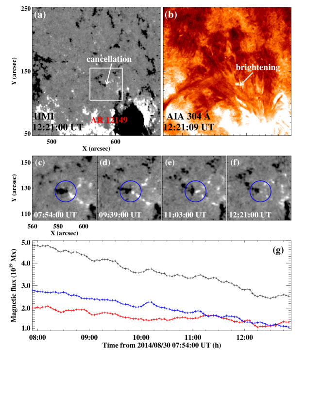
Figure 2.: SDO$/$AIA 304 Å image, HMI LOS magnetograms and temporal variations of the magnetic flux showing the brightening and cancellation process of magnetic fields nearby the filament. The white square in panel (a) displays the FOV of panels (c)-(f). Blue circles outline the area where the temporal evolution of magnetic flux is calculated. The black profile in panel (g) denotes the evolution of total magnetic flux and the red and blue profiles respectively denote the positive and negative magnetic flux.Fig2

Starting from about 08:00 UT, magnetic flux cancellation constantly took place underlying the northern part of the filament (Figure 2). The temporal variations of the cancelling magnetic flux in HMI magnetograms were measured and are displayed in Figure 2(g). We derotated all the magnetograms differentially to a reference time (11:10 UT). The area in which we calculated the magnetic flux is the blue circle in Figures 2(c)-(f). After selection, the pixels with magnetic fields weaker than 10.2 gauss (G) (the noise level determined by Liu et al., 2012) are eliminated. The temporal profiles of positive and negative magnetic flux show a consistent decreasing trend. The total magnetic flux decreased from 4.8$\times$10¹⁹ maxwell (Mx) at 07:54 UT to 2.5$\times$10¹⁹ Mx at 12:55 UT. The average rate of flux cancellation was approximately 1.3$\times$10¹⁵ Mx s^-1. At 12:21 UT, the initial EUV brightening was observed at the location of the cancelled flux and the filament started to erupt (Figure 2(b)).

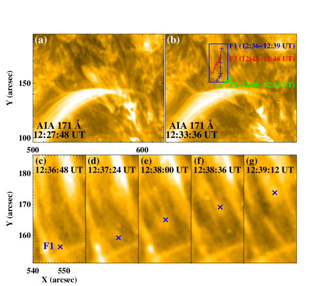
Figure 3.: SDO$/$AIA 171 Å images showing the counterclockwise rotation of the filament (a movie in 171 Å is available as electronic supplementary material). The plus symbols in panel (b) mark the tracks of rotating features (“F1”$-$“F3”). The times in parentheses are the start and end tracking times of the corresponding features. The blue rectangle in panel (b) denotes the FOV of panels (c)-(g). The cross symbols in panels (c)-(g) indicate the positions of “F1” at different times.Fig3

To reveal the rotation of the northern filament more clearly, we tracked three moving features (“F1”$-$“F3” in Figure 3(b)) between 12:36 UT to 12:46 UT. As an example, the evolution of “F1” was shown in Figures 3(c)-(g), exhibiting a helical upward motion. Each track of moving features from the eastern edge to the west corresponds to a rotation angle of about $\pi$, and thus the total twist angle was approximately 3$\pi$ in about 10 min. The average angular speed of the rotating plasma was about 15.7$\times$10^-3 rad s^-1. The filament material ultimately fell back to its initial location from 12:50 UT, and the eruption was failed.

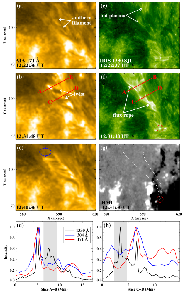
Figure 4.: Panels (a)-(c): helical evolution of the southern filament. The blue ellipse in panel (c) shows the counterclockwise rotation of the filament. Panels (e)-(g): appearance of the flux rope and the corresponding HMI magnetogram. The red circles in panels (f)-(g) outline the southern end of the flux rope. White dotted contour in panel (g) outlines the location of the flux rope. Panels (d) and (h): normalized intensity of the multi-wavelength cuts along slices “A$-$B” and “C$-$D” (red straight lines in panels (b) and (f)), respectively.Fig4

The southern part of the filament showed an obvious helical evolution during the eruption process (Figure 4). Before the appearance of EUV brightening, the southern filament looked linear and showed no helical shape (Figure 4(a)). Afterwards, it was activated and the helical structure gradually appeared (panel (b)). After 12:35 UT, the southern filament showed a rotation motion in the counterclockwise direction (panel (c)). IRIS observations showed that a flux rope with a helical shape appeared at the site of the southern filament (panels (e)-(f)). The comparison of the HMI magnetogram with the 1330 Å image shows that the southern end of the flux rope was rooted in the negative polarity fields of the AR (panels (f)-(g)). In order to compare the multi-wavelength appearances of the flux rope and filament material, the intensity plots along the cuts “A$-$B” and “C$-$D” (red straight lines in panels (b) and (f)) at 12:31:48 UT are presented in the bottom panels of Figure 4. All the cuts along slice “A$-$B” showed a strongest emission at about 5 Mm (first peak in panel (d)). The emission of 1330 Å had a secondary peak at about 7.5 Mm (gray section in panel (d)). However, the cuts of 304 Å and 171 Å show much weaker emissions at about 7.5 Mm. In the 1330 Å cut along slice “C$-$D”, the section corresponding to the filament material, i.e., the gray section in panel (h), showed an intensity enhancement while in the 304 Å and 171 Å cuts, there was a significantly lower emission at the corresponding section. This indicates a striking anti-correlation between the 1330 Å and EUV line intensities at the location of the filament, i.e., peaks of the former correspond to minimum of the latter.

3.2 Flux Rope Observed by the IRIS

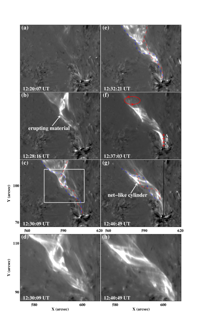
Figure 5.: IRIS base difference 1330 Å slit-jaw images showing the appearance of a flux rope and its helical evolution (a movie is available as electronic supplementary material). The base image is at 12:00 UT. The red and blue dashed curves in panels (c), (e) and (g) outline the fine-scale structures of the flux rope. The white rectangle in panel (c) displays the FOV of the zoomed images in panels (d) and (h). The red ellipse in panel (f) shows the unwinding motion of the flux rope. The four plus symbols (labeled “A”$-$“D”) along the slit in panel (f) mark the locations where we perform detailed analysis of the line profiles in Figure 6.Fig5

Starting from about 12:20 UT, the erupting material of the filament gradually moved southwardly and tracked out bright fine-scale features (Figures 5(a)-(b); a movie is available as electronic supplementary materials). At 12:28 UT, the initial flux rope looked like a funnel and the kink could not be clearly observed (Figure 5(b)). Subsequently, the fine threads were tangled and intertwined with each other. Two individual threads were selected to estimate the twist of the flux rope and they showed crossing several times in an image (red and blue dashed curves in Figure 5(c)). We estimated the amount of twist was about 4$\pi$ according to the geometry of the threads (panels (c)-(d)). At 12:32 UT, the bright plasma arrived at the southern end of the flux rope and illuminated the whole flux rope (panel (e)). The same amount of twist of about 4$\pi$ was visible at this time from the southern footpoint up to the northern part. The length of the visible flux rope was approximately 40^′′. The flux rope was not stable and underwent a counterclockwise rotation around its main axis after 12:35 UT (Figure 5(f)). Initially intertwined strands began to untangle and the morphology of the flux rope was changed evidently. The rotation of the flux rope was obviously the unwinding motion of the twisted magnetic field lines, consistent with the rotation direction of the filament (Figures 3 and 4). Associated with the unwinding motion, the flux rope finally evolved into a “net-like cylinder” (panel (g)), with the southern leg slightly thinner than top parts. The two zoomed images at 12:30 UT and 12:41 UT (panels (d) and (h)) clearly showed the twisted threads of the flux rope. Later on, the intensity of the flux rope decreased and the flux rope became invisible after 12:48 UT.

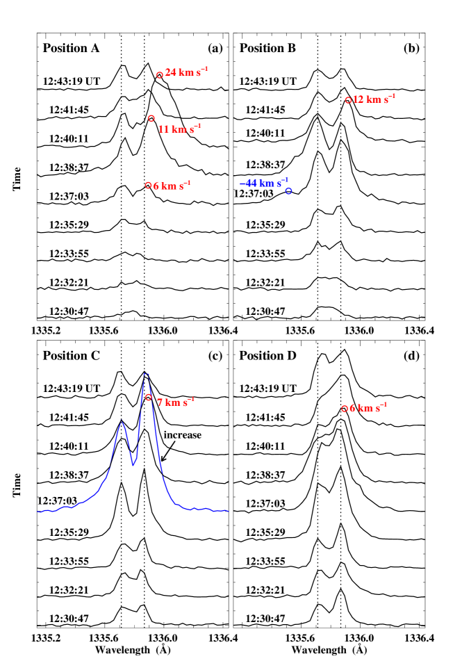
Figure 6.: IRIS line profile evolution of C ii 1335.71 Å at the locations of “A”$-$“D” marked in Figure 5(f). These profiles cover the wavelength range from 1335.14 Å to 1336.44 Å. Two dotted lines in each panel denote two line centers of 1335.71 Å and 1335.86 Å.Fig6

Figure 6 shows the line profile (C ii 1335.71 Å) evolution at different points (locations “A”$-$“D” in Figure 5(f)) along the slit. The slit was located at the southern leg of the flux rope in the SJIs (Figure 5). In the wavelength range of 1335.14$-$1336.44 Å, the line profiles mainly show two peaks at 1335.71 Å and 1335.86 Å. The emissions at locations “A” and “B” between 12:30:47 UT and 12:35:29 UT were relatively weak, compared to those at locations “C” and “D”. By checking the SJIs, we suggest that the weak line profiles of “A” and “B” in the early stage mostly came from the background plasma, and the emissions of southern locations “C” and “D” were from the plasma of the flux rope. Associated with the gradual expansion of the flux rope, the emission intensity of northern locations “A” and “B” increased between 12:37:03 UT and 12:40:11 UT due to the appearance of the flux rope at these locations.

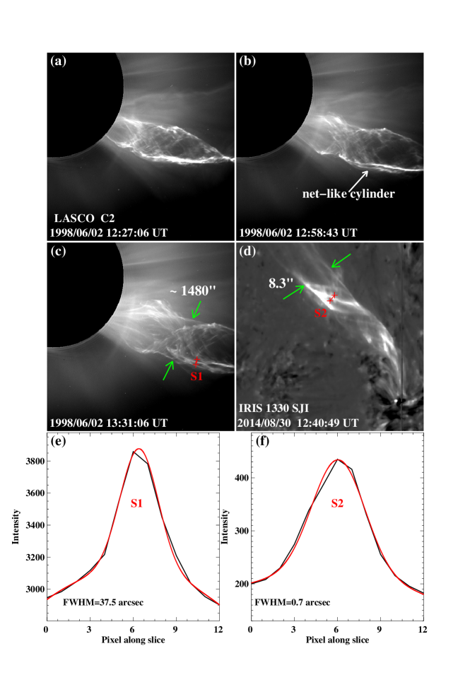
Figure 7.: LASCO/C2 images and IRIS 1330 SJI comparing the CME core on 2 June 1998 with the flux rope, and the Gaussian fitting profiles (panels (e) and (f)) showing the widths of fine-scale structures. Green arrows in panels (c) and (d) point to the location where the widths of the CME core and flux rope are obtained. The red curves in panels (e) and (f) are respectively the Gaussian fitting to the intensity profiles (black ones) along the red slices (Slices “S1” and “S2”) in panels (c) and (d).Fig7

At 12:37:03 UT, the line profile of location “A” showed a redshift of about 6 km s^-1 (panel (a)). Then the Doppler velocity increased to 24 km s^-1 about 3 min later. At 12:40:11 UT, the redshifts at locations “B”$-$“D” were also observed with Doppler velocity of 6$-$12 km s^-1 (panels (b)-(d)), smaller than that of “A”. Moreover, the line profile of location “B” at 12:37:03 UT showed a blue-wing excess (panel (b)), and the minor component contributing about 20% to the total emission. The wing excess corresponded to a strong blueshift of up to 44 km s^-1 (Peter, 2010). By investigating the SJIs, we found a jet-like activity occurred between 12:35:10 UT and 12:37:59 UT. The plasma from the jet possibly accounted for the blueshift at location “B”. For the line profile of location “C” at 12:37:03 UT, the emission intensity rapidly increased to 200% of the peak intensity at 12:35:29 UT (blue line in panel (c)). Meanwhile, the line width increased evidently. This might be caused by the transient heating process of the local plasma.

3.3 Comparison of the Flux Rope with the CME on 2 June 1998

The morphology of the flux rope reminded us of a CME on 2 June 1998. In LASCO/C2 observations, the CME core was composed of many fine-scale structures, which were crossed and tangled with each other (Figure 7(a)). The CME core had a cylindrical shape with helical field lines wrapping around it (Figures 7(b) and (c)), similar to the shape of the flux rope (Figure 7(d)). However, the scales of the CME core and the flux rope were greatly different. The CME core had a width of 1480^′′ (green arrows in Figure 7(c)), equal to 1.54 $R_{\odot}$. The width of the flux rope was approximately 8.3^′′ (green arrows in Figure 7(d)). We also measured the widths of fine structures (slices “S1” for the CME core and “S2” for the flux rope in Figures 7(c)-(d)) by using Gaussian function to fit the intensity profiles. The full width at half maximum (FWHW) of the Gaussian fitting profile was thought to be the width of fine-scale structure. The fine structure of the CME core had a width of 37.5^′′ (Figure 7(e)), about 4.5 times of the width of the entire flux rope (8.3^′′). The fine structure of the flux rope was only 0.7^′′ wide, nearly 4 pixels of IRIS images.

4 Summary and Discussion

We report the observations of a flux rope at TR temperatures made by IRIS on 30 August 2014 nearby AR 12149. The flux rope was located at the southern part of an erupting filament based on the SDO observations. Initially magnetic flux cancellation and obvious EUV brightenings were observed. Then the filament was activated and the bright material moved southward and filled in the body of the flux rope observed at 1330 Å. The fine structures of the flux rope were tangled with each other, and the total twist was estimated to be almost 4$\pi$. Afterwards, the flux rope exhibited a counterclockwise unwinding motion (when viewed top-down) around its main axis. Spectral observations displayed that the redshifts from several to more than 20 km s^-1 appeared at the southern leg of the flux rope in the late stage. The flux rope showed a helical structure, similar to the CME core of 2 June 1998. However, the spatial scales of the flux rope and the CME core are greatly different.

Magnetic flux cancellation constantly occurred in about 5 h before the appearance of the flux rope. We suggest that the magnetic flux cancellation initiated reconnection and some activation of the flux rope. The obvious EUV brightenings indicate that heating took place during the filament eruption. The heated plasma from the filament moved towards its southern end and illuminated the flux rope body in the 1330 Å channel. Thus the twisted structures of the flux rope were tracked out by filling it with hot and dense plasma. We suggest that part of the magnetic flux rope structures may exist in the space filled in by the flux ropes before the appearance of the flux rope. This is similar to the observations of Raouafi (2009) and Li and Zhang (2013b), who reported the brightening of flux ropes and the appearance of the fine structures due to the nearby flares or other activities.

The filament material showed the counterclockwise rotation motion along the helical flux rope structures in the late stage. The total twist (4$\pi$) of the flux rope is above the critical value (2.5$\pi$$-$3.5$\pi$; Hood and Priest, 1981), which indicates that kink instability possibly took place in this event. The rotation was obviously the unwinding motion of the twisted magnetic field lines. The stored twist and magnetic helicity of the flux rope were possibly transported to the ambient open fields (Liu et al., 2009; Chen et al., 2012; Zhang et al., 2015). The average angular speed (15.7$\times$10^-3 rad s^-1) of the flux rope is comparable to that of the unwinding jet (11.1$\times$10^-3 rad s^-1) presented by Shen et al. (2011). Koleva et al. (2012) reported the twist of an eruptive filament by 6$\pi$ and suggested that kink instability played a key role in the filament eruption.

The IRIS slit covered the fine-scale structures at the western side of the axis and the line profiles of C ii at these locations were mostly redshifted. The spectroscopic results are consistent with the above inferred counter-clockwise rotations, with dominant redshifts on the west. The redshifts at the northern locations are larger than the south (in positions “A” and “D”). There might be two reasons to explain the difference in the redshifts. The southern locations were near to the footpoints of the flux rope and had a smaller rotating radius. Moreover, the Doppler shifts at different locations along the same helical structure are different due to the projection effect, i.e., the points at the edge of the helical structure had the largest Doppler shifts and the points in the middle had the lower velocities. Su et al. (2014) revealed the opposite Doppler velocities of $\approx$ 5 km s^-1 at the two sides of the prominence, indicating the rotational motion of the magnetic structures in tornado-like prominences. Liu et al. (2015) investigated an eruptive prominence by using IRIS observations and found the blue to redshift transition with height and sinusoidal spectral variations along the slit during the counter-clockwise unwinding motions.

The small-scale flux rope (width of 8.3^′′) and the large-scale CME core (width of 1.54 $R_{\odot}$) on 2 June 1998 both showed a helical structure. They look very similar possibly because of low optical density, and the fine-scale structures at both sides of the flux rope are visible. This similarity shows the presence of flux ropes of different scales on the Sun. The fine structure of the flux rope is about 0.7^′′ wide, similar to the previous results. Li and Zhang (2013b) showed that the flux ropes in EUV wavelengths are composed of about 100 fine-scale structures, with an average width of about 1.6^′′. Yang et al. (2014) analyzed a flux rope in H$\alpha$ images and measured the average width of its individual threads of 1.11 Mm. The fine structure of the CME core has a width of about 37.5^′′, much thicker than that of the flux rope.

The comparison of multi-wavelength observations showed that some threads of the flux rope emitted only in spectral lines at TR temperatures, e.g., C ii. The structures of the flux rope could not be clearly observed in high-temperature wavelengths such as 171 and 304 Å. This suggests that some plasma of the flux rope is heated to only 25000 K, rather than a higher temperature. The comprehensive characteristics of flux ropes at TR temperatures need to be analyzed in further studies, together with the comparison of low- and high-temperature flux ropes.

Acknowledgements

IRIS is a NASA small explorer mission developed and operated by LMSAL with mission operations executed at NASA Ames Research center and major contributions to downlink communications funded by the Norwegian Space Center (NSC, Norway) through an ESA PRODEX contract. We acknowledge the SDO/AIA and HMI for providing data. This work is supported by the National Basic Research Program of China under grant 2011CB811403, the National Natural Science Foundations of China (11303050, 11025315, 11221063 and 11003026), the CAS Project KJCX2-EW-T07 and the Strategic Priority Research Program$-$The Emergence of Cosmological Structures of the Chinese Academy of Sciences, Grant No. XDB09000000.

References

- (1) Amari, T., Aly, J.-J., Mikic, Z., Linker, J.: 2010, ApJ 717, L26.
- (2) Aulanier, G., Török, T., Démoulin, P., DeLuca, E. E.: 2010, ApJ 708, 314.
- (3) Brueckner, G. E., Howard, R. A., Koomen, M. J., Korendyke, C. M., Michels, D. J., Moses, J. D., et al.: 1995, Sol. Phys. 162, 357.
- (4) Canou, A., Amari, T.: 2010, ApJ 715, 1566.
- (5) Chen, B., Bastian, T. S., Gary, D. E.: 2014a, ApJ 794, 149.
- (6) Chen, H., Zhang, J., Cheng, X., Ma, S., Yang, S., Li, T.: 2014b, ApJ 797, L15.
- (7) Chen, H.-D., Zhang, J., Ma, S.-L.: 2012, Res. Astron. Astrophys. 12, 573.
- (8) Cheng, X., Ding, M. D., Zhang, J., Sun, X. D., Guo, Y., Wang, Y. M., Kliem, B., Deng, Y. Y.: 2014, ApJ 789, 93.
- (9) De Pontieu, B., Title, A. M., Lemen, J. R., Kushner, G. D., Akin, D. J., Allard, B., et al.: 2014, Sol. Phys. 289, 2733.
- (10) Fan, Y.: 2005, ApJ 630, 543.
- (11) Fan, Y., Gibson, S. E.: 2004, ApJ 609, 1123.
- (12) Guo, Y., Ding, M. D., Schmieder, B., et al.: 2010, ApJ 725, L38.
- (13) Harvey, J. W., Bolding, J., Clark, R., Li, H., Török, T., Wiegelmann, T.: 2011, Bull. Am. Astron. Soc., 1745.
- (14) Hood, A. W., Priest, E. R.: 1981, Geophys. Astrophys. Fluid Dyn. 17, 297.
- (15) Ji, H., Wang, H., Schmahl, E. J., Moon, Y.-J., Jiang, Y.: 2003, ApJ 595, L135.
- (16) Joshi, N. C., Magara, T., Inoue, S.: 2014a, ApJ 795, 4.
- (17) Joshi, N. C., Srivastava, A. K., Filippov, B., Kayshap, P., Uddin, W., Chandra, R., Choudhary, D. P., Dwivedi, B. N.: 2014b, ApJ 787, 11.
- (18) Koleva, K., Madjarska, M. S., Duchlev, P., et al.: 2012, A&A 540, AA127.
- (19) Kumar, P., Cho, K.-S.: 2014, A&A 572, AA83.
- (20) Kumar, P., Srivastava, A. K., Filippov, B., Uddin, W.: 2010, Sol. Phys. 266, 39.
- (21) Lemen, J. R., Title, A. M., Akin, D. J., Boerner, P. F., Chou, C., Drake, J. F., et al.: 2012, Sol. Phys. 275, 17.
- (22) Li, L. P., Peter, H., Chen, F., Zhang, J.: 2014, A&A 570, 93.
- (23) Li, L., Zhang, J.: 2013a, A&A 552, L11.
- (24) Li, T., Zhang, J.: 2013b, ApJ 770, L25.
- (25) Li, T., Zhang, J.: 2013c, ApJ 778, L29.
- (26) Li, T., Zhang, J.: 2014, ApJ 791, L13.
- (27) Lites, B. W.: 2005, ApJ 622, 1275.
- (28) Liu, R., Alexander, D., Gilbert, H. R.: 2007, ApJ 661, 1260.
- (29) Liu, Y., Hoeksema, J. T., Scherrer, P. H., Schou, J., Couvidat, S., Bush, R. I., Duvall, T. L., Hayashi, K., Sun, X., Zhao, X.: 2012, Sol. Phys. 279, 295.
- (30) Liu, W., Berger, T. E., Title, A. M., Tarbell, T. D.: 2009, ApJ 707, L37.
- (31) Liu, W., De Pontieu, B., Vial, J.-C., Vial, J.-C., Title, A. M., Carlsson, M., et al.: 2015, ApJ 803, 85.
- (32) Moore, R. L., Sterling, A. C., Hudson, H. S., Lemen, J. R.: 2001, ApJ 552, 833.
- (33) O’Dwyer, B., Del Zanna, G., Mason, H. E., Weber, M. A., Tripathi, D.: 2010, A&A 521, 21.
- (34) Okamoto, T. J., Tsuneta, S., Lites, B. W., Kubo, M., Yokoyama, T., Berger, T. E., et al.: 2008, ApJ 673, L215.
- (35) Pesnell, W. D., Thompson, B. J., Chamberlin, P. C.: 2012, Sol. Phys. 275, 3.
- (36) Peter, H.: 2010, A&A 521, A51.
- (37) Pneuman, G. W.: 1983, Sol. Phys. 88, 219.
- (38) Raouafi, N.-E. 2009, ApJ 691, L128.
- (39) Rust, D. M., Kumar, A.: 1994, Sol. Phys. 155, 69.
- (40) Rust, D. M., LaBonte, B. J.: 2005, ApJ 622, L69.
- (41) Scherrer, P. H., Schou, J., Bush, R. I., Kosovichev, A. G., Bogart, R. S., Hoeksema, J. T., et al.: 2012, Sol. Phys. 275, 207.
- (42) Shen, Y., Liu, Y., Su, J., Ibrahim, A.: 2011, ApJ 735, L43.
- (43) Song, H. Q., Zhang, J., Chen, Y., Cheng, X.: 2014, ApJ 792, L40.
- (44) Srivastava, A. K., Zaqarashvili, T. V., Kumar, P., Khodachenko, M. L.: 2010, ApJ 715, 292.
- (45) Su, Y., Gömöry, P., Veronig, A., Temmer, M., Wang, T. J., Vanninathan, K., Gan, W. Q., Li, Y. P.: 2014, ApJ 785, L2.
- (46) Tian, H., DeLuca, E., Reeves, K. K., McKillop, S., De Pontieu, B., Martinez-Sykora, J., et al.: 2014, ApJ 786, 137.
- (47) Török, T., Kliem, B.: 2003, A&A 406, 1043.
- (48) Török, T., Kliem, B.: 2005, ApJ 630, L97.
- (49) van Ballegooijen, A. A., Martens, P. C. H.: 1989, ApJ 343, 971.
- (50) Vourlidas, A., Syntelis, P., Tsinganos, K.: 2012, Sol. Phys. 280, 509.
- (51) Yan, X. L., Xue, Z. K., Liu, J. H., Kong, D. F., Xu, C. L.: 2014, ApJ 782, 67.
- (52) Yang, S., Zhang, J., Liu, Z., Xiang, Y.: 2014, ApJ 784, L36.
- (53) Zhang, Q. M., Ning, Z. J., Guo, Y., Zhou, T. H., Cheng, X., Ji, H. S., Feng, L., Wiegelmann, T.: 2015, ApJ 805, 4.
- (54) Zheng, R., Jiang, Y., Yang, J., Bi, Y., Hong, J., Yang, D., Yang, B.: 2012, ApJ 753, 112.