Neutrino seesaw mechanism with texture zeros

Jiajun Liao1,3, D. Marfatia1,3, and K. Whisnant2,3

1Department of Physics and Astronomy, University of Hawaii at Manoa, Honolulu, HI 96822, USA
2Department of Physics and Astronomy, Iowa State University, Ames, IA 50011, USA
3Kavli Institute for Theoretical Physics, University of California, Santa Barbara, CA 93106, USA
Abstract

In the context of the Type I seesaw mechanism, we carry out a systematic study of the constraints that result from zeros in both the Dirac and right-handed Majorana neutrino mass matrices. We find that most constraints can be expressed in the standard form with one or two element/cofactor zeros alone, while there are 9 classes of nonstandard constraints. We show that all the constraints are stable under one-loop renormalization group running from the lightest right-handed neutrino mass scale to the electroweak scale. We study the predictions of the nonstandard constraints for the lightest neutrino mass, Dirac CP phase and neutrinoless double beta decay.

1 Introduction

Many Standard Model (SM) extensions predict the existence of right-handed (RH) Majorana neutrinos, which are often used to explain neutrino masses via the Type I seesaw mechanism [1]. The effective mass matrix of the light Majorana neutrinos is given by

M=MDMR1MDT,𝑀subscript𝑀𝐷superscriptsubscript𝑀𝑅1superscriptsubscript𝑀𝐷𝑇\displaystyle M=-M_{D}{M_{R}}^{-1}M_{D}^{T}\,, (1)

where MDsubscript𝑀𝐷M_{D} and MRsubscript𝑀𝑅M_{R} are the mass matrices for the Dirac and RH Majorana neutrinos, respectively.

In the basis where the charged lepton mass matrix is diagonal, the light neutrino mass matrix is described by 9 real parameters and can be written as [2]

M=Vdiag(m1,m2,m3)V,𝑀superscript𝑉diagsubscript𝑚1subscript𝑚2subscript𝑚3superscript𝑉M=V^{*}\text{diag}(m_{1},m_{2},m_{3})V^{\dagger}\,, (2)

where the misubscript𝑚𝑖m_{i} are real and nonnegative, V=Udiag(1,eiϕ2/2,eiϕ3/2)𝑉𝑈diag1superscript𝑒𝑖subscriptitalic-ϕ22superscript𝑒𝑖subscriptitalic-ϕ32V=U\text{diag}(1,e^{i\phi_{2}/2},e^{i\phi_{3}/2}), and

U=[c13c12c13s12s13eiδs12c23c12s23s13eiδc12c23s12s23s13eiδs23c13s12s23c12c23s13eiδc12s23s12c23s13eiδc23c13].𝑈matrixsubscript𝑐13subscript𝑐12subscript𝑐13subscript𝑠12subscript𝑠13superscript𝑒𝑖𝛿subscript𝑠12subscript𝑐23subscript𝑐12subscript𝑠23subscript𝑠13superscript𝑒𝑖𝛿subscript𝑐12subscript𝑐23subscript𝑠12subscript𝑠23subscript𝑠13superscript𝑒𝑖𝛿subscript𝑠23subscript𝑐13subscript𝑠12subscript𝑠23subscript𝑐12subscript𝑐23subscript𝑠13superscript𝑒𝑖𝛿subscript𝑐12subscript𝑠23subscript𝑠12subscript𝑐23subscript𝑠13superscript𝑒𝑖𝛿subscript𝑐23subscript𝑐13\displaystyle U=\begin{bmatrix}c_{13}c_{12}&c_{13}s_{12}&s_{13}e^{-i\delta}\\ -s_{12}c_{23}-c_{12}s_{23}s_{13}e^{i\delta}&c_{12}c_{23}-s_{12}s_{23}s_{13}e^{i\delta}&s_{23}c_{13}\\ s_{12}s_{23}-c_{12}c_{23}s_{13}e^{i\delta}&-c_{12}s_{23}-s_{12}c_{23}s_{13}e^{i\delta}&c_{23}c_{13}\end{bmatrix}\,. (3)

After decades of neutrino oscillation experiments, five parameters (three mixing angles and two mass-squared differences) in the neutrino sector have been determined to rather good precision. However, the hierarchy of the three light neutrino masses is still unknown, and there are two possibilities: (i) m1<m2<m3subscript𝑚1subscript𝑚2subscript𝑚3m_{1}<m_{2}<m_{3} for the normal hierarchy (NH) and (ii) m3<m1<m2subscript𝑚3subscript𝑚1subscript𝑚2m_{3}<m_{1}<m_{2} for the inverted hierarchy (IH). The remaining four unknown parameters may be taken as the lightest mass (m1subscript𝑚1m_{1} for the NH, or m3subscript𝑚3m_{3} for the IH), the Dirac CP phase δ𝛿\delta and two Majorana phases (ϕ1subscriptitalic-ϕ1\phi_{1} and ϕ2subscriptitalic-ϕ2\phi_{2}). The Dirac phase and the mass hierarchy will be measured in future neutrino oscillation experiments, and the lightest mass can in principle be determined from beta decay experiments and cosmological observations.

Of the many neutrino mixing models proposed in the literature, texture zero models [3] are attractive because of the simple relations on the matrix elements that are found in these models. Texture zero constraints can be imposed on the light neutrino mass matrix directly. However, in the context of the Type I seesaw mechanism, since the light mass matrix is a product of the Dirac mass matrix and the RH neutrino mass matrix, it is natural to consider texture zeros in the Dirac and RH neutrino mass matrices [4]. Zeros in the Dirac and RH neutrino mass matrix can be realized from discrete Nsubscript𝑁\mathbb{Z}_{N} symmetries with suitable scalar singlets [5].

In this paper, we carry out a systematic study of the constraints that result from various zero textures in both the Dirac and RH Majorana mass matrices in the context of the Type I seesaw mechanism. We find that most cases lead to the standard constraints which can be expressed in the form of just one or two element/cofactor zeros, which have been studied extensively in the literature [6, 7, 8, 9, 10, 11, 12]. However, there are also 9 classes of nonstandard constraints, i.e., constraints which are not described by simple texture or cofactor zeros in the light neutrino mass matrix. We first show that both the standard and nonstandard constraints are stable under one-loop renormalization group equation (RGE) running from the lightest RH neutrino mass scale M1subscript𝑀1M_{1} to the electroweak scale MZsubscript𝑀𝑍M_{Z}. Then we study the phenomenological implications of the nonstandard constraints using recent data measured by neutrino oscillation experiments. We find that some cases are excluded, and for the rest we obtain preferred values for the lightest mass and Dirac CP phase, which will be probed in the next generation of neutrino experiments. We also study neutrinoless double beta decay for the nonstandard constraints.

This paper is organized as follows. In Section 2, we explore the constraints of zero textures in the seesaw mechanism. In Section 3, we discuss RGE effects on the constraints. In Section 4, we study the phenomenological implications of the nonstandard constraints and summarize our results in Section 5.

2 Classes of constraints

We consider three generations of RH Majorana neutrinos and we assume MRsubscript𝑀𝑅M_{R} is not singular. Since the Majorana mass matrix is symmetric, there are 6 independent matrix elements in MRsubscript𝑀𝑅M_{R}, and 9 independent elements in MDsubscript𝑀𝐷M_{D}. For a case with NRsubscript𝑁𝑅N_{R} zeros in MRsubscript𝑀𝑅M_{R} and NDsubscript𝑁𝐷N_{D} zeros in MDsubscript𝑀𝐷M_{D}, there are should be at least N6𝑁6N-6 complex constraints on the elements of M𝑀M, where N=NR+ND𝑁subscript𝑁𝑅subscript𝑁𝐷N=N_{R}+N_{D} is the total number of zeros element. This may be understood as follows.

We start with 15=6+9156915=6+9 nonzero complex parameters in MRsubscript𝑀𝑅M_{R} and MDsubscript𝑀𝐷M_{D}, respectively. There are a total of N𝑁N zeros in MRsubscript𝑀𝑅M_{R} and MDsubscript𝑀𝐷M_{D}, so that leaves 15N15𝑁15-N independent complex parameters. We can always insert a diagonal matrix between MRsubscript𝑀𝑅M_{R} and MDsubscript𝑀𝐷M_{D} (and the same matrix between MRsubscript𝑀𝑅M_{R} and MDTsuperscriptsubscript𝑀𝐷𝑇M_{D}^{T}), which effectively absorbs 3 complex parameters (or, putting it another way, there are 3 relative normalizations that are redundant in the prediction of the light neutrino mass matrix from the seesaw mechanism). This leaves us with 12 - N independent complex parameters. In M𝑀M there are 6 independent elements, so the net number of constraints on the elements of M𝑀M is 6(12N)=N6612𝑁𝑁66-(12-N)=N-6. In terms of real parameters, we have 242N242𝑁24-2N, from which we can subtract 3 unphysical phases, leaving us with 212N212𝑁21-2N physical real parameters in M𝑀M. Since there are 9 real parameters in the neutrino sector and 5 of them are well determined, in general, if N9𝑁9N\geq 9, the model will be over constrained and if N6𝑁6N\leq 6, the model will be unconstrained.

This counting rule only gives the minimum number of constraints. There are accidental constraints that result from some special combinations of texture zeros in MDsubscript𝑀𝐷M_{D} and MRsubscript𝑀𝑅M_{R}, e.g., if MDsubscript𝑀𝐷M_{D} has a column or a submatrix composed of all zeros, then the constraint detM=0𝑀0\det M=0 always exists regardless of the counting rule. So in order to obtain all the constraints for a given zero structure of MDsubscript𝑀𝐷M_{D} and MRsubscript𝑀𝑅M_{R}, we have to make sure all of the independent constraints are obtained. Our analysis proceeds as follows.

We scan all possible texture zero structures for MDsubscript𝑀𝐷M_{D}. Since M𝑀M is invariant under a permutation of the columns and rows of MRsubscript𝑀𝑅M_{R} with a simultaneous permutation of the corresponding columns of MDsubscript𝑀𝐷M_{D}, we only consider one representative structure for each set of MRsubscript𝑀𝑅M_{R} that are equivalent under permutation. For each combination of MDsubscript𝑀𝐷M_{D} and MRsubscript𝑀𝑅M_{R}, we check all the elements and cofactors, and the determinant of M𝑀M using Eq. (1) and look for independent constraints. We write the constraints in terms of the elements, cofactors or determinant of M𝑀M in the simplest form. The experimental data does not allow more than two zeros in the elements or cofactors of the light mass matrix, hence we only consider cases that give less than three such zeros. The cases that give a block diagonal mass matrix are also ignored because they lead to a zero mixing angle, which is excluded by current experimental data. For the other cases, we analyze the elements of M𝑀M, and make sure we obtain all of the independent constraints. We find that most constraints can be expressed in the standard form that can be written in terms of just one or two element/cofactor zeros, but there are also nine nonstandard constraints, which are listed in Table 1. The structures that lead to the nonstandard constraints are provided in Appendix A. Classes 2, 3, 4 and 5 are discussed in Ref. [4], with constraint equations in a different (albeit equivalent) form. Classes 1 and 9 are subsets of well-known models with the additional constraint detM=0𝑀0\det M=0. Classes 6, 7 and 8 are new and not previously discussed in the literature.

Table 1: Classes of the nonstandard constraints that can not be expressed in terms of one or two element (Mαβsubscript𝑀𝛼𝛽M_{\alpha\beta}) or cofactor (Cαβsubscript𝐶𝛼𝛽C_{\alpha\beta}) zeros alone. Here αβγ𝛼𝛽𝛾\alpha\neq\beta\neq\gamma, and no sum is implied in the constraint equations.
Class NR+NDsubscript𝑁𝑅subscript𝑁𝐷N_{R}+N_{D} Nonstandard constraints No. of constraints
1 4+5454+5 Mαα=Mββ=0subscript𝑀𝛼𝛼subscript𝑀𝛽𝛽0M_{\alpha\alpha}=M_{\beta\beta}=0 and detM=0𝑀0\det M=0 3
2 4+4444+4, 3+5353+5, 3+4343+4, 2+5252+5 Mαα=0subscript𝑀𝛼𝛼0M_{\alpha\alpha}=0 and detM=0𝑀0\det M=0 3
3 3+5353+5 Mαβ=0subscript𝑀𝛼𝛽0M_{\alpha\beta}=0 and detM=0𝑀0\det M=0 3
4 4+4444+4 Mαα=0subscript𝑀𝛼𝛼0M_{\alpha\alpha}=0 and MββMαγ=2MαβMβγsubscript𝑀𝛽𝛽subscript𝑀𝛼𝛾2subscript𝑀𝛼𝛽subscript𝑀𝛽𝛾M_{\beta\beta}M_{\alpha\gamma}=2M_{\alpha\beta}M_{\beta\gamma} 6
5 3+5353+5 Cαα=0subscript𝐶𝛼𝛼0C_{\alpha\alpha}=0 and CββCαγ=2CαβCβγsubscript𝐶𝛽𝛽subscript𝐶𝛼𝛾2subscript𝐶𝛼𝛽subscript𝐶𝛽𝛾C_{\beta\beta}C_{\alpha\gamma}=2C_{\alpha\beta}C_{\beta\gamma} 6
6 4+3434+3, 3+4343+4, 2+5252+5 MααCαα=detMsubscript𝑀𝛼𝛼subscript𝐶𝛼𝛼𝑀M_{\alpha\alpha}C_{\alpha\alpha}=\det M 3
7 4+3434+3 Mαα2Cαα=4MαβMαγCβγsuperscriptsubscript𝑀𝛼𝛼2subscript𝐶𝛼𝛼4subscript𝑀𝛼𝛽subscript𝑀𝛼𝛾subscript𝐶𝛽𝛾M_{\alpha\alpha}^{2}C_{\alpha\alpha}=4M_{\alpha\beta}M_{\alpha\gamma}C_{\beta\gamma} 3
8 3+4343+4 MββdetM=Mαβ2Cααsubscript𝑀𝛽𝛽𝑀superscriptsubscript𝑀𝛼𝛽2subscript𝐶𝛼𝛼M_{\beta\beta}\det M=-M_{\alpha\beta}^{2}C_{\alpha\alpha} 6
9 4+3434+3, 3+4343+4, 2+5252+5 detM=0𝑀0\det M=0 1

3 Renormalization group running

The neutrino mixing parameters are measured at low energies, while the effective mass matrix of Eq. (1) can arise at a much high energy scale. The evolution of the light neutrino masses from the lightest RH neutrino mass scale M1subscript𝑀1M_{1} to the electroweak scale MZsubscript𝑀𝑍M_{Z} is described by the one-loop RGE [13],

16π2dMdt=κM+η[(YlYl)M+M(YlYl)T],16superscript𝜋2𝑑𝑀𝑑𝑡𝜅𝑀𝜂delimited-[]subscript𝑌𝑙superscriptsubscript𝑌𝑙𝑀𝑀superscriptsubscript𝑌𝑙superscriptsubscript𝑌𝑙𝑇16\pi^{2}\frac{dM}{dt}=\kappa M+\eta[(Y_{l}Y_{l}^{\dagger})M+M(Y_{l}Y_{l}^{\dagger})^{T}]\,, (4)

where t=ln(Λ/M1)𝑡Λsubscript𝑀1t=\ln(\Lambda/M_{1}), ΛΛ\Lambda is the renormalization scale and Yl=diag(ye,yμ,yτ)subscript𝑌𝑙diagsubscript𝑦𝑒subscript𝑦𝜇subscript𝑦𝜏Y_{l}=\text{diag}(y_{e},y_{\mu},y_{\tau}) with yαsubscript𝑦𝛼y_{\alpha} being the eigenvalues of the charged lepton Yukawa coupling matrix. In the SM,

η=32,κ3g22+6yt2+λ,formulae-sequence𝜂32𝜅3superscriptsubscript𝑔226superscriptsubscript𝑦𝑡2𝜆\displaystyle\eta=-\frac{3}{2}\,,\quad\kappa\approx-3g_{2}^{2}+6y_{t}^{2}+\lambda\,, (5)

and in the Minimal Supersymmetric Standard Model (MSSM),

η=1,κ65g126g22+6yt2,formulae-sequence𝜂1𝜅65superscriptsubscript𝑔126superscriptsubscript𝑔226superscriptsubscript𝑦𝑡2\displaystyle\eta=1\,,\quad\kappa\approx-\frac{6}{5}g_{1}^{2}-6g_{2}^{2}+6y_{t}^{2}\,, (6)

where g1,g2subscript𝑔1subscript𝑔2g_{1},g_{2} are the gauge couplings, ytsubscript𝑦𝑡y_{t} is the top quark Yukawa coupling, and λ𝜆\lambda is the Higgs self-coupling.

The solution to Eq. (4) can be written in the form [14],

M(MZ)=I0[Ie000Iμ000Iτ]M(M1)[Ie000Iμ000Iτ],𝑀subscript𝑀𝑍subscript𝐼0matrixsubscript𝐼𝑒000subscript𝐼𝜇000subscript𝐼𝜏𝑀subscript𝑀1matrixsubscript𝐼𝑒000subscript𝐼𝜇000subscript𝐼𝜏M(M_{Z})=I_{0}\begin{bmatrix}I_{e}&0&0\\ 0&I_{\mu}&0\\ 0&0&I_{\tau}\end{bmatrix}M(M_{1})\begin{bmatrix}I_{e}&0&0\\ 0&I_{\mu}&0\\ 0&0&I_{\tau}\end{bmatrix}, (7)

where

I0=exp[116π20ln(M1/MZ)κ(t)𝑑t],subscript𝐼0116superscript𝜋2superscriptsubscript0subscript𝑀1subscript𝑀𝑍𝜅𝑡differential-d𝑡I_{0}=\exp\left[-\frac{1}{16\pi^{2}}\int_{0}^{\ln(M_{1}/M_{Z})}\kappa(t)dt\right], (8)

and

Il=exp[η16π20ln(M1/MZ)yl2(t)𝑑t],subscript𝐼𝑙𝜂16superscript𝜋2superscriptsubscript0subscript𝑀1subscript𝑀𝑍superscriptsubscript𝑦𝑙2𝑡differential-d𝑡I_{l}=\exp\left[-\frac{\eta}{16\pi^{2}}\int_{0}^{\ln(M_{1}/M_{Z})}y_{l}^{2}(t)dt\right], (9)

for l=e,μ,τ𝑙𝑒𝜇𝜏l=e,\mu,\tau.

From Eq. (7), we see that RGE running can be described by multiplying the elements of the mass matrix by three factors, i.e.,

Mαβ=MαβI0IαIβ,subscript𝑀𝛼𝛽subscriptsuperscript𝑀𝛼𝛽subscript𝐼0subscript𝐼𝛼subscript𝐼𝛽\displaystyle M_{\alpha\beta}=M^{\prime}_{\alpha\beta}I_{0}I_{\alpha}I_{\beta}\,, (10)

where α,β=e,μ,τformulae-sequence𝛼𝛽𝑒𝜇𝜏\alpha,\beta=e,\mu,\tau, M𝑀M and Msuperscript𝑀M^{\prime} are the effective mass matrix at the electroweak scale and the lightest RH neutrino mass scale, respectively. Taking the inverse of Eq. (7), we get

(M1)αβ=(M1)αβ1I0IαIβ.subscriptsuperscript𝑀1𝛼𝛽subscriptsuperscript𝑀1𝛼𝛽1subscript𝐼0subscript𝐼𝛼subscript𝐼𝛽\displaystyle(M^{-1})_{\alpha\beta}=(M^{\prime-1})_{\alpha\beta}\frac{1}{I_{0}I_{\alpha}I_{\beta}}\,. (11)

Since Cαβ=detM(M1)αβsubscript𝐶𝛼𝛽𝑀subscriptsuperscript𝑀1𝛼𝛽C_{\alpha\beta}=\det M(M^{-1})_{\alpha\beta}, it is easy to verify that both the standard and nonstandard constraints are stable under one-loop renormalization group running from M1subscript𝑀1M_{1} to MZsubscript𝑀𝑍M_{Z}.

Note that above the lightest RH neutrino mass, one must consider seesaw threshold effects, which can lead to large corrections to θ12subscript𝜃12\theta_{12} and the Dirac and Majorana phases [13]. Due to these effects, some textures that are excluded by data may be allowed above the seesaw threshold [15]. Estimating the effect of RGE running above M1subscript𝑀1M_{1} on low-energy parameters is beyond the scope of this paper because additional assumptions about the Yukawa coupling matrix and the RH Majorana mass matrix need to be invoked [16].

It has been shown that the two-loop RGE can change the rank of the light neutrino mass matrix [17], which implies that the constraint detM=0𝑀0\det M=0 is not stable at two loop. In the SM, two-loop effects can be described by adding an additional term to Eq. (4[18], so that

16π2dMdt=κM+η[(YlYl)M+M(YlYl)T]+216π2(YlYl)M(YlYl)T.16superscript𝜋2𝑑𝑀𝑑𝑡𝜅𝑀𝜂delimited-[]subscript𝑌𝑙superscriptsubscript𝑌𝑙𝑀𝑀superscriptsubscript𝑌𝑙superscriptsubscript𝑌𝑙𝑇216superscript𝜋2subscript𝑌𝑙superscriptsubscript𝑌𝑙𝑀superscriptsubscript𝑌𝑙superscriptsubscript𝑌𝑙𝑇16\pi^{2}\frac{dM}{dt}=\kappa M+\eta[(Y_{l}Y_{l}^{\dagger})M+M(Y_{l}Y_{l}^{\dagger})^{T}]+\frac{2}{16\pi^{2}}(Y_{l}Y_{l}^{\dagger})M(Y_{l}Y_{l}^{\dagger})^{T}\,. (12)

The solution to the two-loop RGE is [19]

M(MZ)=I0[MeeIe2IeeMeμIeIμIeμMeτIeIτIeτMeμIeIμIeμMμμIμ2IμμMμτIμIτIμτMeτIeIτIeτMμτIμIτIμτMττIτ2Iττ],𝑀subscript𝑀𝑍subscript𝐼0matrixsubscriptsuperscript𝑀𝑒𝑒superscriptsubscript𝐼𝑒2subscript𝐼𝑒𝑒subscriptsuperscript𝑀𝑒𝜇subscript𝐼𝑒subscript𝐼𝜇subscript𝐼𝑒𝜇subscriptsuperscript𝑀𝑒𝜏subscript𝐼𝑒subscript𝐼𝜏subscript𝐼𝑒𝜏subscriptsuperscript𝑀𝑒𝜇subscript𝐼𝑒subscript𝐼𝜇subscript𝐼𝑒𝜇subscriptsuperscript𝑀𝜇𝜇superscriptsubscript𝐼𝜇2subscript𝐼𝜇𝜇subscriptsuperscript𝑀𝜇𝜏subscript𝐼𝜇subscript𝐼𝜏subscript𝐼𝜇𝜏subscriptsuperscript𝑀𝑒𝜏subscript𝐼𝑒subscript𝐼𝜏subscript𝐼𝑒𝜏subscriptsuperscript𝑀𝜇𝜏subscript𝐼𝜇subscript𝐼𝜏subscript𝐼𝜇𝜏subscriptsuperscript𝑀𝜏𝜏superscriptsubscript𝐼𝜏2subscript𝐼𝜏𝜏M(M_{Z})=I_{0}\begin{bmatrix}M^{\prime}_{ee}I_{e}^{2}I_{ee}&M^{\prime}_{e\mu}I_{e}I_{\mu}I_{e\mu}&M^{\prime}_{e\tau}I_{e}I_{\tau}I_{e\tau}\\ M^{\prime}_{e\mu}I_{e}I_{\mu}I_{e\mu}&M^{\prime}_{\mu\mu}I_{\mu}^{2}I_{\mu\mu}&M^{\prime}_{\mu\tau}I_{\mu}I_{\tau}I_{\mu\tau}\\ M^{\prime}_{e\tau}I_{e}I_{\tau}I_{e\tau}&M^{\prime}_{\mu\tau}I_{\mu}I_{\tau}I_{\mu\tau}&M^{\prime}_{\tau\tau}I_{\tau}^{2}I_{\tau\tau}\end{bmatrix}, (13)

where

Imn=exp[2(16π2)20ln(M1/MZ)ym2(t)yn2(t)𝑑t],subscript𝐼𝑚𝑛2superscript16superscript𝜋22superscriptsubscript0subscript𝑀1subscript𝑀𝑍superscriptsubscript𝑦𝑚2𝑡superscriptsubscript𝑦𝑛2𝑡differential-d𝑡I_{mn}=\exp\left[-\frac{2}{(16\pi^{2})^{2}}\int_{0}^{\ln(M_{1}/M_{Z})}y_{m}^{2}(t)y_{n}^{2}(t)dt\right], (14)

for m,n=e,μ,τformulae-sequence𝑚𝑛𝑒𝜇𝜏m,n=e,\mu,\tau. We see that the nonstandard constraints are not stable under two-loop running. However, as shown in Ref. [18], the two-loop correction to the lightest mass is of order 1013superscript101310^{-13} eV in the SM and 1010(tanβ/10)4superscript1010superscript𝛽10410^{-10}(\tan\beta/10)^{4} eV in the MSSM. Two-loop effects can also generate a tiny value for θ13subscript𝜃13\theta_{13} at the level of 10121014superscript1012superscript101410^{-12}-10^{-14} in the SM [19]. Considering current uncertainties in the oscillation parameters, two-loop corrections do not affect our numerical results.

4 Phenomenology of the nonstandard constraints

The phenomenology of the standard constraints have been studied extensively in the literature; for recent analyses, see Ref. [6] for one element zero, Ref. [7] for one off-diagonal element/cofactor zero, and Ref. [8] for one diagonal element/cofactor zero. The results for two element/cofactor zeros can be found in Ref. [9]; other recent analyses can be found in Ref. [10] for two element zeros, Ref. [11] for two cofactor zeros, and Ref. [12] for one element zero and one cofactor zero. Here we focus on the phenomenology of the nonstandard constraints.

4.1 Classes 1, 2, 3, 9: det M = 0

Structures with the constraint detM=0𝑀0\det M=0 are easiest to analyze. Since detM=0𝑀0\det M=0 is equivalent to m1=0subscript𝑚10m_{1}=0 (m3=0subscript𝑚30m_{3}=0) for the NH (IH), the oscillation parameters are not affected, and these models are the same as models that have already been studied, with the additional constraint that the lightest mass is zero. For Class 9, detM=0𝑀0\det M=0 is the only constraint and therefore any value of δ𝛿\delta is allowed (see Sec. 5 for a discussion of the possible constraints from neutrinoless double beta decay). For models with constraints besides detM=0𝑀0\det M=0, we only need to check the parameter space allowed by the additional constraints and see if m1=0subscript𝑚10m_{1}=0 (m3=0subscript𝑚30m_{3}=0) is allowed for the NH (IH).

Class 1 constraints have the same number of parameters as the most economical seesaw model [20]. From Ref. [9], we know that if two diagonal elements are both equal to zero, only Mμμ=Mττ=0subscript𝑀𝜇𝜇subscript𝑀𝜏𝜏0M_{\mu\mu}=M_{\tau\tau}=0 for the IH is allowed, but in this case the 2σ2𝜎2\sigma allowed region does not include m3=0subscript𝑚30m_{3}=0. Hence, Class 1 is not allowed by the experimental data at 2σ2𝜎2\sigma.

For Class 2, from Ref. [8] we know that only Mμμ=0subscript𝑀𝜇𝜇0M_{\mu\mu}=0 or Mττ=0subscript𝑀𝜏𝜏0M_{\tau\tau}=0 are allowed for the IH at 2σ2𝜎2\sigma when the lightest mass is zero. Similarly, for Class 3, from Ref. [7] we know that only Meμ=0subscript𝑀𝑒𝜇0M_{e\mu}=0 or Meτ=0subscript𝑀𝑒𝜏0M_{e\tau}=0 are allowed for the IH at 2σ2𝜎2\sigma when the lightest mass is zero. In all other cases with exactly one texture zero in the light neutrino mass matrix, a massless neutrino is excluded at 2σ2𝜎2\sigma. Hence only four cases in Class 2 and 3 are allowed for the IH at 2σ2𝜎2\sigma, and none for the NH. The allowed cases in Class 2 are: (i) Mμμ=0subscript𝑀𝜇𝜇0M_{\mu\mu}=0, and detM=0𝑀0\det M=0; (ii) Mττ=0subscript𝑀𝜏𝜏0M_{\tau\tau}=0, and detM=0𝑀0\det M=0. The allowed cases in Class 3 are: (i) Meμ=0subscript𝑀𝑒𝜇0M_{e\mu}=0, and detM=0𝑀0\det M=0; (ii) Meτ=0subscript𝑀𝑒𝜏0M_{e\tau}=0, and detM=0𝑀0\det M=0. We note that the Class 2 and 3 constraints have been noted in Ref. [4] as Eqs. (48) and (49). Our results for the allowed cases are consistent with Ref. [4].

Reference [4] also lists the conditions detM=0𝑀0\det M=0 and MααMββ(Mαβ)2=0subscript𝑀𝛼𝛼subscript𝑀𝛽𝛽superscriptsubscript𝑀𝛼𝛽20M_{\alpha\alpha}M_{\beta\beta}-(M_{\alpha\beta})^{2}=0 (as Eq. 50) and Mαα=Mαβ=0subscript𝑀𝛼𝛼subscript𝑀𝛼𝛽0M_{\alpha\alpha}=M_{\alpha\beta}=0 and (M1)αα=0subscriptsuperscript𝑀1𝛼𝛼0(M^{-1})_{\alpha\alpha}=0 (as Eq. 51) as new constraints. The structures that lead to these conditions have six and three cofactor zeros, respectively. We do not count them as nonstandard constraints because a light neutrino mass matrix with more than two cofactor zeros has already been shown to be excluded by experimental data.

4.2 Class 4

Our Class 4 constraints are equivalent to Mαα=0subscript𝑀𝛼𝛼0M_{\alpha\alpha}=0, Mββ(M1)ββ=1subscript𝑀𝛽𝛽subscriptsuperscript𝑀1𝛽𝛽1M_{\beta\beta}(M^{-1})_{\beta\beta}=1 and (M1)γγ0subscriptsuperscript𝑀1𝛾𝛾0(M^{-1})_{\gamma\gamma}\neq 0 obtained in Ref. [4] as Eq. (51). We demonstrate this equivalency below.

Since Mαα=0subscript𝑀𝛼𝛼0M_{\alpha\alpha}=0,

detM=2MαβMβγMαγ(Mαγ)2Mββ(Mαβ2)2Mγγ.𝑀2subscript𝑀𝛼𝛽subscript𝑀𝛽𝛾subscript𝑀𝛼𝛾superscriptsubscript𝑀𝛼𝛾2subscript𝑀𝛽𝛽superscriptsuperscriptsubscript𝑀𝛼𝛽22subscript𝑀𝛾𝛾\displaystyle\det M=2M_{\alpha\beta}M_{\beta\gamma}M_{\alpha\gamma}-(M_{\alpha\gamma})^{2}M_{\beta\beta}-(M_{\alpha\beta}^{2})^{2}M_{\gamma\gamma}\,. (15)

Plugging MββMαγ=2MαβMβγsubscript𝑀𝛽𝛽subscript𝑀𝛼𝛾2subscript𝑀𝛼𝛽subscript𝑀𝛽𝛾M_{\beta\beta}M_{\alpha\gamma}=2M_{\alpha\beta}M_{\beta\gamma} into the above equation, we get

detM=(Mαβ2)2Mγγ.𝑀superscriptsuperscriptsubscript𝑀𝛼𝛽22subscript𝑀𝛾𝛾\displaystyle\det M=-(M_{\alpha\beta}^{2})^{2}M_{\gamma\gamma}\,. (16)

Also, since Mαα=0subscript𝑀𝛼𝛼0M_{\alpha\alpha}=0, we have (M1)γγ=(Mαβ)2detMsubscriptsuperscript𝑀1𝛾𝛾superscriptsubscript𝑀𝛼𝛽2𝑀(M^{-1})_{\gamma\gamma}=-\frac{(M_{\alpha\beta})^{2}}{\det M}, and therefore

Mγγ(M1)γγ=1.subscript𝑀𝛾𝛾subscriptsuperscript𝑀1𝛾𝛾1\displaystyle M_{\gamma\gamma}(M^{-1})_{\gamma\gamma}=1\,. (17)

Together with Mαα=0subscript𝑀𝛼𝛼0M_{\alpha\alpha}=0 and Mββ0subscript𝑀𝛽𝛽0M_{\beta\beta}\neq 0 (which is implicitly included in our constraints), we see Class 4 constraints are consistent with the conditions (52) in Ref. [4]. The form of the constraint in Table 1 has the merit of being quadratic instead of cubic (as in Ref. [4]), which allows for easier numerical analysis.

The constraints Mαα=0subscript𝑀𝛼𝛼0M_{\alpha\alpha}=0 and MββMαγ=2MαβMβγsubscript𝑀𝛽𝛽subscript𝑀𝛼𝛾2subscript𝑀𝛼𝛽subscript𝑀𝛽𝛾M_{\beta\beta}M_{\alpha\gamma}=2M_{\alpha\beta}M_{\beta\gamma} can be written as

X1+σX2+ρX3=0,subscript𝑋1𝜎subscript𝑋2𝜌subscript𝑋30X_{1}+\sigma X_{2}+\rho X_{3}=0\,, (18)

and

A1+σ2A2+ρ2A3+σA12+ρA13+σρA23=0,subscript𝐴1superscript𝜎2subscript𝐴2superscript𝜌2subscript𝐴3𝜎subscript𝐴12𝜌subscript𝐴13𝜎𝜌subscript𝐴230A_{1}+\sigma^{2}A_{2}+\rho^{2}A_{3}+\sigma A_{12}+\rho A_{13}+\sigma\rho A_{23}=0\,, (19)

where σ=(m2/m1)eiϕ2𝜎subscript𝑚2subscript𝑚1superscript𝑒𝑖subscriptitalic-ϕ2\sigma=(m_{2}/m_{1})e^{-i\phi_{2}}, ρ=(m3/m1)eiϕ3𝜌subscript𝑚3subscript𝑚1superscript𝑒𝑖subscriptitalic-ϕ3\rho=(m_{3}/m_{1})e^{-i\phi_{3}}, Xi=Uαi2subscript𝑋𝑖superscriptsubscript𝑈𝛼𝑖absent2X_{i}=U_{\alpha i}^{*2}, Ai=Uβi2UαiUγisubscript𝐴𝑖superscriptsubscript𝑈𝛽𝑖absent2superscriptsubscript𝑈𝛼𝑖superscriptsubscript𝑈𝛾𝑖A_{i}=U_{\beta i}^{*2}U_{\alpha i}^{*}U_{\gamma i}^{*} and Aij=2UβiUβj(UαiUγj+UαjUγi)(Uβi2UαjUγj+Uβj2UαiUγi)subscript𝐴𝑖𝑗2superscriptsubscript𝑈𝛽𝑖superscriptsubscript𝑈𝛽𝑗superscriptsubscript𝑈𝛼𝑖superscriptsubscript𝑈𝛾𝑗superscriptsubscript𝑈𝛼𝑗superscriptsubscript𝑈𝛾𝑖superscriptsubscript𝑈𝛽𝑖absent2superscriptsubscript𝑈𝛼𝑗superscriptsubscript𝑈𝛾𝑗superscriptsubscript𝑈𝛽𝑗absent2superscriptsubscript𝑈𝛼𝑖superscriptsubscript𝑈𝛾𝑖A_{ij}=2U_{\beta i}^{*}U_{\beta j}^{*}(U_{\alpha i}^{*}U_{\gamma j}^{*}+U_{\alpha j}^{*}U_{\gamma i}^{*})-(U_{\beta i}^{*2}U_{\alpha j}^{*}U_{\gamma j}^{*}+U_{\beta j}^{*2}U_{\alpha i}^{*}U_{\gamma i}^{*}) for i=1,2,3𝑖123i=1,2,3. Since Eq. (19) is quadratic, it can be solved with Eq. (18). We get

ρ𝜌\displaystyle\rho =A23X1X2X3A13X22X32A2X1X32+A12X2X32±X2Λ2X3[A3X22+X3(A2X3A23X2)],absentplus-or-minussubscript𝐴23subscript𝑋1subscript𝑋2subscript𝑋3subscript𝐴13superscriptsubscript𝑋22subscript𝑋32subscript𝐴2subscript𝑋1superscriptsubscript𝑋32subscript𝐴12subscript𝑋2superscriptsubscript𝑋32subscript𝑋2Λ2subscript𝑋3delimited-[]subscript𝐴3superscriptsubscript𝑋22subscript𝑋3subscript𝐴2subscript𝑋3subscript𝐴23subscript𝑋2\displaystyle=\frac{A_{23}X_{1}X_{2}X_{3}-A_{13}X_{2}^{2}X_{3}-2A_{2}X_{1}X_{3}^{2}+A_{12}X_{2}X_{3}^{2}\pm X_{2}\sqrt{\Lambda}}{2X_{3}[A_{3}X_{2}^{2}+X_{3}(A_{2}X_{3}-A_{23}X_{2})]}\,, (20)
σ𝜎\displaystyle\sigma =A23X1X3+A13X2X32A3X1X2A12X32Λ2[A3X22+X3(A2X3A23X2)],absentminus-or-plussubscript𝐴23subscript𝑋1subscript𝑋3subscript𝐴13subscript𝑋2subscript𝑋32subscript𝐴3subscript𝑋1subscript𝑋2subscript𝐴12superscriptsubscript𝑋32Λ2delimited-[]subscript𝐴3superscriptsubscript𝑋22subscript𝑋3subscript𝐴2subscript𝑋3subscript𝐴23subscript𝑋2\displaystyle=\frac{A_{23}X_{1}X_{3}+A_{13}X_{2}X_{3}-2A_{3}X_{1}X_{2}-A_{12}X_{3}^{2}\mp\sqrt{\Lambda}}{2[A_{3}X_{2}^{2}+X_{3}(A_{2}X_{3}-A_{23}X_{2})]}\,, (21)

where Λ=[2A3X1X2+X3(A12X3A23X1A13X2)]24[A3X12+X3(A1X3A13X1)][A3X22+X3(A2X3A23X2)]Λsuperscriptdelimited-[]2subscript𝐴3subscript𝑋1subscript𝑋2subscript𝑋3subscript𝐴12subscript𝑋3subscript𝐴23subscript𝑋1subscript𝐴13subscript𝑋224delimited-[]subscript𝐴3superscriptsubscript𝑋12subscript𝑋3subscript𝐴1subscript𝑋3subscript𝐴13subscript𝑋1delimited-[]subscript𝐴3superscriptsubscript𝑋22subscript𝑋3subscript𝐴2subscript𝑋3subscript𝐴23subscript𝑋2\Lambda=[2A_{3}X_{1}X_{2}+X_{3}(A_{12}X_{3}-A_{23}X_{1}-A_{13}X_{2})]^{2}-4[A_{3}X_{1}^{2}+X_{3}(A_{1}X_{3}-A_{13}X_{1})][A_{3}X_{2}^{2}+X_{3}(A_{2}X_{3}-A_{23}X_{2})]. Taking the absolute values of σ𝜎\sigma and ρ𝜌\rho, we find m2/m1subscript𝑚2subscript𝑚1m_{2}/m_{1} and m3/m1subscript𝑚3subscript𝑚1m_{3}/m_{1}. Then m1subscript𝑚1m_{1} can be written as

m1subscript𝑚1\displaystyle m_{1} =δm2|σ|21=12δm2±Δm2|ρ|21,absent𝛿superscript𝑚2superscript𝜎21plus-or-minus12𝛿superscript𝑚2Δsuperscript𝑚2superscript𝜌21\displaystyle=\sqrt{\frac{\delta m^{2}}{|\sigma|^{2}-1}}=\sqrt{\frac{\frac{1}{2}\delta m^{2}\pm\Delta m^{2}}{|\rho|^{2}-1}}\,, (22)

where the plus (minus) sign in Eq. (22) is for the NH (IH).

Our numerical analysis proceeds as follows. Since there are 5 independent parameters in the light mass matrix in this case, we take them to be θ12subscript𝜃12\theta_{12}, θ23subscript𝜃23\theta_{23}, θ13subscript𝜃13\theta_{13}, δm2m22m12𝛿superscript𝑚2superscriptsubscript𝑚22superscriptsubscript𝑚12\delta m^{2}\equiv m_{2}^{2}-m_{1}^{2} and Δm2m32(m12+m22)/2Δsuperscript𝑚2superscriptsubscript𝑚32superscriptsubscript𝑚12superscriptsubscript𝑚222\Delta m^{2}\equiv m_{3}^{2}-(m_{1}^{2}+m_{2}^{2})/2. First, we choose a set of the five oscillation parameters within the 2σ2𝜎2\sigma range from a recent global fit [21]. Then we solve Eq. (22) by scanning over δ𝛿\delta from 0 to 360superscript360360^{\circ}. We sample 105superscript10510^{5} sets of oscillation parameters allowed at 2σ2𝜎2\sigma; by keeping the values of m1subscript𝑚1m_{1} and δ𝛿\delta that are allowed, we obtain the allowed regions in m1δsubscript𝑚1𝛿m_{1}-\delta (m3δsubscript𝑚3𝛿m_{3}-\delta) plane for the NH (IH).

The allowed cases in Class 4 are as follows:

  1. 1.

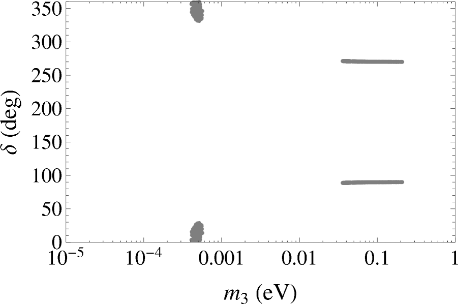
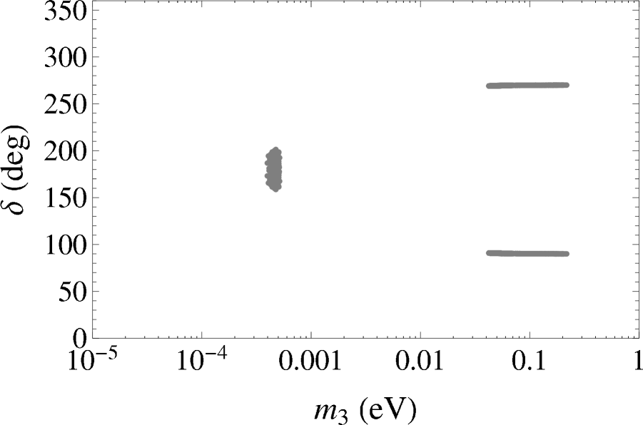
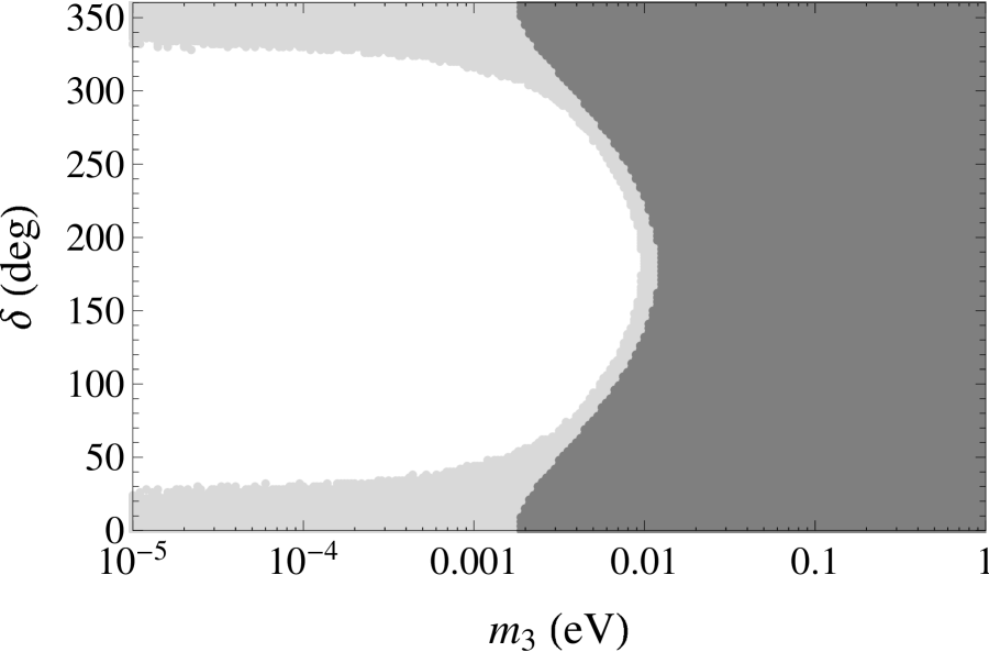
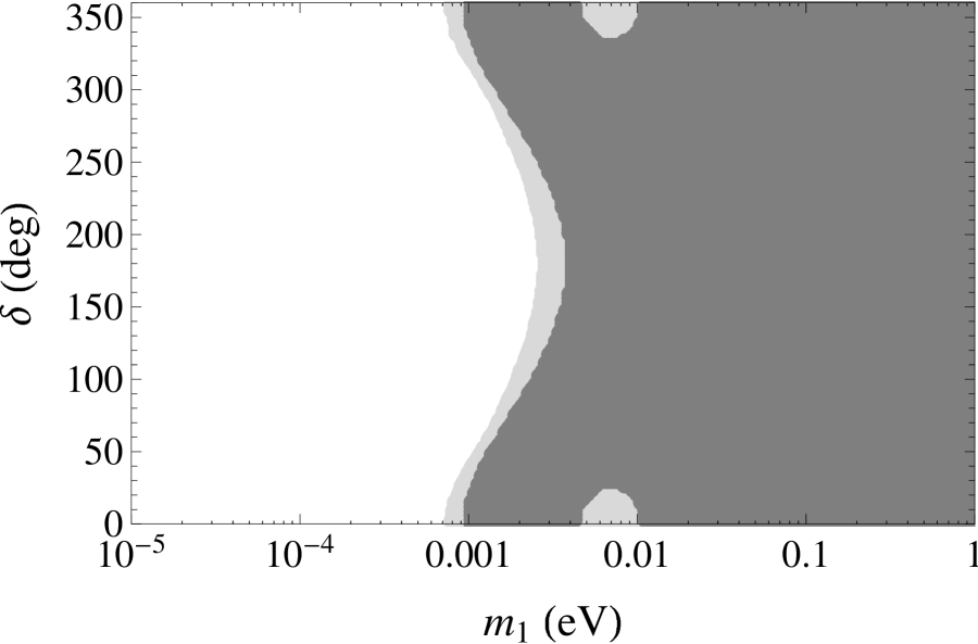
    Mμμ=0subscript𝑀𝜇𝜇0M_{\mu\mu}=0 and MττMeμ=2MμτMeτsubscript𝑀𝜏𝜏subscript𝑀𝑒𝜇2subscript𝑀𝜇𝜏subscript𝑀𝑒𝜏M_{\tau\tau}M_{e\mu}=2M_{\mu\tau}M_{e\tau}. This case is allowed for both hierarchies. The allowed regions are shown in Fig. 1.

    Refer to caption
    Refer to caption
    Figure 1: The 2σ2𝜎2\sigma allowed regions in the plane of the lightest mass and Dirac phase for the constraints, Mμμ=0subscript𝑀𝜇𝜇0M_{\mu\mu}=0 and MττMeμ=2MμτMeτsubscript𝑀𝜏𝜏subscript𝑀𝑒𝜇2subscript𝑀𝜇𝜏subscript𝑀𝑒𝜏M_{\tau\tau}M_{e\mu}=2M_{\mu\tau}M_{e\tau}. The left (right) panel is for the normal (inverted) hierarchy.
  2. 2.

    Mττ=0subscript𝑀𝜏𝜏0M_{\tau\tau}=0 and MμμMeτ=2MμτMeμsubscript𝑀𝜇𝜇subscript𝑀𝑒𝜏2subscript𝑀𝜇𝜏subscript𝑀𝑒𝜇M_{\mu\mu}M_{e\tau}=2M_{\mu\tau}M_{e\mu}. This case is allowed for both hierarchies. The allowed regions are shown in Fig. 2. They are similar to Fig. 1 with δδ+180𝛿𝛿superscript180\delta\rightarrow\delta+180^{\circ} for both hierarchies. The similarity is explained by the approximate μτ𝜇𝜏\mu-\tau symmetry of the experimental data.

Refer to caption
Refer to caption
Figure 2: Same as Fig. 1, except for Mττ=0subscript𝑀𝜏𝜏0M_{\tau\tau}=0 and MμμMeτ=2MμτMeμsubscript𝑀𝜇𝜇subscript𝑀𝑒𝜏2subscript𝑀𝜇𝜏subscript𝑀𝑒𝜇M_{\mu\mu}M_{e\tau}=2M_{\mu\tau}M_{e\mu}.

Note that these allowed regions are consistent with the results obtained in Ref. [4], in which 3σ𝜎\sigma ranges of each parameter are used as input.

4.3 Class 5

Similar to Class 4, Class 5 constraints are consistent with the conditions (M1)αα=0subscriptsuperscript𝑀1𝛼𝛼0(M^{-1})_{\alpha\alpha}=0, Mββ(M1)ββ=1subscript𝑀𝛽𝛽subscriptsuperscript𝑀1𝛽𝛽1M_{\beta\beta}(M^{-1})_{\beta\beta}=1 and Mγγ0subscript𝑀𝛾𝛾0M_{\gamma\gamma}\neq 0 in Eq. (53) of Ref. [4]. We find that it is easier to use the quadratic form of Class 5 constraints for the numerical analysis.

Similar to Eqs. (18) and (19), the two constraints Cαα=0subscript𝐶𝛼𝛼0C_{\alpha\alpha}=0 and CββCβγ=2CαβCαγsubscript𝐶𝛽𝛽subscript𝐶𝛽𝛾2subscript𝐶𝛼𝛽subscript𝐶𝛼𝛾C_{\beta\beta}C_{\beta\gamma}=2C_{\alpha\beta}C_{\alpha\gamma} can be written as

X1+X2/σ+X3/ρ=0,subscript𝑋1subscript𝑋2superscript𝜎subscript𝑋3superscript𝜌0X_{1}+X_{2}/\sigma^{*}+X_{3}/\rho^{*}=0\,, (23)

and

A1+A2/(σ)2+A3/(ρ)2+A12/σ+A13/ρ+A23/(σρ)=0,subscript𝐴1subscript𝐴2superscriptsuperscript𝜎2subscript𝐴3superscriptsuperscript𝜌2subscript𝐴12superscript𝜎subscript𝐴13superscript𝜌subscript𝐴23superscript𝜎superscript𝜌0A_{1}+A_{2}/(\sigma^{*})^{2}+A_{3}/(\rho^{*})^{2}+A_{12}/\sigma^{*}+A_{13}/\rho^{*}+A_{23}/(\sigma^{*}\rho^{*})=0\,, (24)

where ρ𝜌\rho, σ𝜎\sigma, Xisubscript𝑋𝑖X_{i}, Aisubscript𝐴𝑖A_{i} and Aijsubscript𝐴𝑖𝑗A_{ij} are defined after Eq. (19). The analysis of this case follows that of Class 4 with the replacements, σ1/σ𝜎1superscript𝜎\sigma\rightarrow 1/\sigma^{*} and ρ1/ρ𝜌1superscript𝜌\rho\rightarrow 1/\rho^{*}. The allowed cases in Class 5 are as follows:

  1. 1.

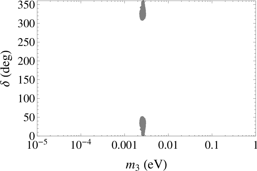
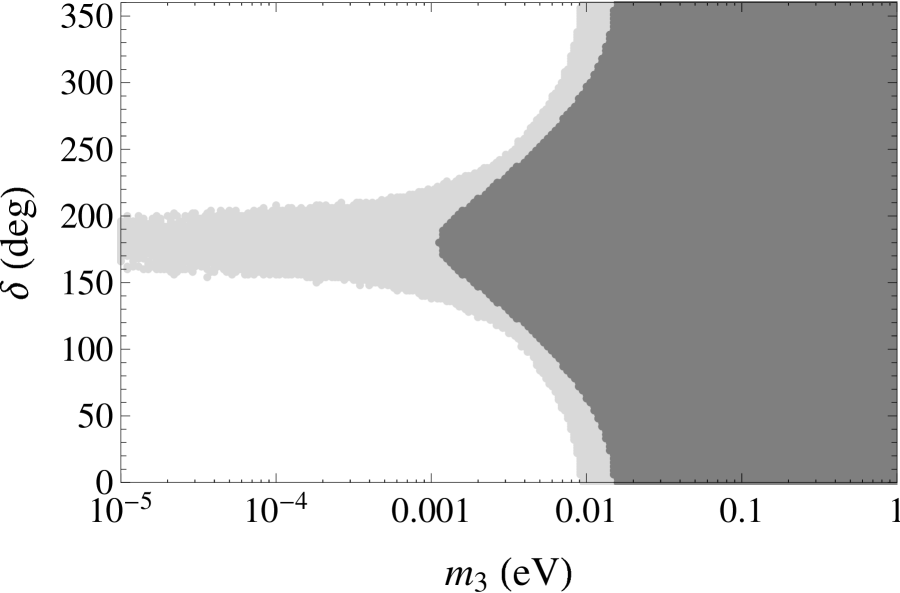
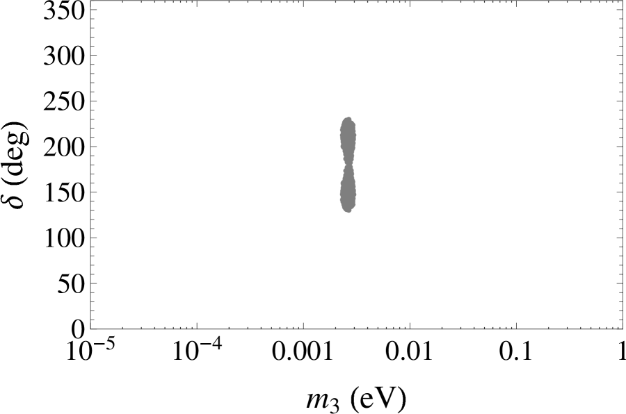
    Cee=0subscript𝐶𝑒𝑒0C_{ee}=0 and CμμCeτ=2CeμCμτsubscript𝐶𝜇𝜇subscript𝐶𝑒𝜏2subscript𝐶𝑒𝜇subscript𝐶𝜇𝜏C_{\mu\mu}C_{e\tau}=2C_{e\mu}C_{\mu\tau}. This case is allowed for the IH only. The allowed regions are shown in the left panel of Fig. 3.
    Refer to caption
    Refer to caption
    Figure 3: The 2σ2𝜎2\sigma allowed regions in the (m3,δ)subscript𝑚3𝛿(m_{3},\delta) plane for the inverted hierarchy. The left (right) panel shows the results for the constraints, Cee=0subscript𝐶𝑒𝑒0C_{ee}=0 and CμμCeτ=2CeμCμτsubscript𝐶𝜇𝜇subscript𝐶𝑒𝜏2subscript𝐶𝑒𝜇subscript𝐶𝜇𝜏C_{\mu\mu}C_{e\tau}=2C_{e\mu}C_{\mu\tau} (CττCeμ=2CeτCμτsubscript𝐶𝜏𝜏subscript𝐶𝑒𝜇2subscript𝐶𝑒𝜏subscript𝐶𝜇𝜏C_{\tau\tau}C_{e\mu}=2C_{e\tau}C_{\mu\tau}).
  2. 2.

    Cee=0subscript𝐶𝑒𝑒0C_{ee}=0 and CττCeμ=2CeτCμτsubscript𝐶𝜏𝜏subscript𝐶𝑒𝜇2subscript𝐶𝑒𝜏subscript𝐶𝜇𝜏C_{\tau\tau}C_{e\mu}=2C_{e\tau}C_{\mu\tau}. This case is allowed for the IH only. The allowed regions are shown in the right panel of Fig. 3, which is similar to the left panel with δδ+180𝛿𝛿superscript180\delta\rightarrow\delta+180^{\circ} because of the approximate μτ𝜇𝜏\mu-\tau symmetry.

  3. 3.

    Cμμ=0subscript𝐶𝜇𝜇0C_{\mu\mu}=0 and CττCeμ=2CμτCeτsubscript𝐶𝜏𝜏subscript𝐶𝑒𝜇2subscript𝐶𝜇𝜏subscript𝐶𝑒𝜏C_{\tau\tau}C_{e\mu}=2C_{\mu\tau}C_{e\tau}. This case is allowed for both hierarchies. The allowed regions are shown in Fig. 4.

    Refer to caption
    Refer to caption
    Figure 4: Same as Fig. 1, except for Cμμ=0subscript𝐶𝜇𝜇0C_{\mu\mu}=0 and CττCeμ=2CμτCeτsubscript𝐶𝜏𝜏subscript𝐶𝑒𝜇2subscript𝐶𝜇𝜏subscript𝐶𝑒𝜏C_{\tau\tau}C_{e\mu}=2C_{\mu\tau}C_{e\tau}.
  4. 4.

    Cττ=0subscript𝐶𝜏𝜏0C_{\tau\tau}=0 and CμμCeτ=2CμτCeμsubscript𝐶𝜇𝜇subscript𝐶𝑒𝜏2subscript𝐶𝜇𝜏subscript𝐶𝑒𝜇C_{\mu\mu}C_{e\tau}=2C_{\mu\tau}C_{e\mu}. This case is allowed for both hierarchies. The allowed regions are similar to Fig. 4 with δδ+180𝛿𝛿superscript180\delta\rightarrow\delta+180^{\circ} for both hierarchies. The similarity can be explained by the approximate μτ𝜇𝜏\mu-\tau symmetry of the experimental data.

Note that these allowed regions are consistent with the results obtained in Ref. [4]. Also, the Class 4 constraints are dual to the Class 5 constraints because they have the same functional form with the roles of elements and cofactors reversed [22]. From Ref. [22], we know that the allowed regions of Class 4 and 5 should be similar for opposite mass hierarchies when the lightest mass is larger than about 20 meV. This can be seen from the left panel of Fig. 1 and the right panel of Fig. 4, and from the right panel of Fig. 1 and the left panel of Fig. 4.

4.4 Class 6

Since detM0𝑀0\det M\neq 0, the constraint MααCαα=detMsubscript𝑀𝛼𝛼subscript𝐶𝛼𝛼𝑀M_{\alpha\alpha}C_{\alpha\alpha}=\det M is equivalent to Mαα(M1)αα=1subscript𝑀𝛼𝛼subscriptsuperscript𝑀1𝛼𝛼1M_{\alpha\alpha}(M^{-1})_{\alpha\alpha}=1, which can be written as

(m1Uα12+m2Uα22eiϕ2+m3Uα32eiϕ3)(m11Uα12+m21Uα22eiϕ2+m31Uα32eiϕ3)=1.subscript𝑚1superscriptsubscript𝑈𝛼1absent2subscript𝑚2superscriptsubscript𝑈𝛼2absent2superscript𝑒𝑖subscriptitalic-ϕ2subscript𝑚3superscriptsubscript𝑈𝛼3absent2superscript𝑒𝑖subscriptitalic-ϕ3superscriptsubscript𝑚11superscriptsubscript𝑈𝛼12superscriptsubscript𝑚21superscriptsubscript𝑈𝛼22superscript𝑒𝑖subscriptitalic-ϕ2superscriptsubscript𝑚31superscriptsubscript𝑈𝛼32superscript𝑒𝑖subscriptitalic-ϕ31\displaystyle(m_{1}U_{\alpha 1}^{*2}+m_{2}U_{\alpha 2}^{*2}e^{-i\phi_{2}}+m_{3}U_{\alpha 3}^{*2}e^{-i\phi_{3}})(m_{1}^{-1}U_{\alpha 1}^{2}+m_{2}^{-1}U_{\alpha 2}^{2}e^{i\phi_{2}}+m_{3}^{-1}U_{\alpha 3}^{2}e^{i\phi_{3}})=1\,. (25)

Defining Uαj=|Uαj|eiβjsubscript𝑈𝛼𝑗subscript𝑈𝛼𝑗superscript𝑒𝑖𝛽𝑗U_{\alpha j}=|U_{\alpha j}|e^{i\beta j} and ϕj=ϕj+2βj2β1,subscriptsuperscriptitalic-ϕ𝑗subscriptitalic-ϕ𝑗2subscript𝛽𝑗2subscript𝛽1\phi^{\prime}_{j}=\phi_{j}+2\beta_{j}-2\beta_{1}\,, we absorb the phases of the U𝑈U’s into ϕjsubscriptitalic-ϕ𝑗\phi_{j}’s and write Eq. (25) as

(m1|Uα1|2+m2|Uα2|2eiϕ2+m3|Uα3|2eiϕ3)(m11|Uα1|2+m21|Uα2|2eiϕ2+m31|Uα3|2eiϕ3)=1.subscript𝑚1superscriptsubscript𝑈𝛼12subscript𝑚2superscriptsubscript𝑈𝛼22superscript𝑒𝑖subscriptsuperscriptitalic-ϕ2subscript𝑚3superscriptsubscript𝑈𝛼32superscript𝑒𝑖subscriptsuperscriptitalic-ϕ3superscriptsubscript𝑚11superscriptsubscript𝑈𝛼12superscriptsubscript𝑚21superscriptsubscript𝑈𝛼22superscript𝑒𝑖superscriptitalic-ϕ2superscriptsubscript𝑚31superscriptsubscript𝑈𝛼32superscript𝑒𝑖superscriptitalic-ϕ31\displaystyle(m_{1}|U_{\alpha 1}|^{2}+m_{2}|U_{\alpha 2}|^{2}e^{-i\phi^{\prime}_{2}}+m_{3}|U_{\alpha 3}|^{2}e^{-i\phi^{\prime}_{3}})(m_{1}^{-1}|U_{\alpha 1}|^{2}+m_{2}^{-1}|U_{\alpha 2}|^{2}e^{i\phi^{\prime}2}+m_{3}^{-1}|U_{\alpha 3}|^{2}e^{i\phi^{\prime}3})=1\,. (26)

We now expand the above equation into real and imaginary parts, and after some simplification we get

|Uα1|4+|Uα2|4+|Uα3|4+|Uα2|2|Uα3|2(m2m3+m3m2)(cosϕ2cosϕ3+sinϕ2sinϕ3)superscriptsubscript𝑈𝛼14superscriptsubscript𝑈𝛼24superscriptsubscript𝑈𝛼34superscriptsubscript𝑈𝛼22superscriptsubscript𝑈𝛼32subscript𝑚2subscript𝑚3subscript𝑚3subscript𝑚2subscriptsuperscriptitalic-ϕ2subscriptsuperscriptitalic-ϕ3subscriptsuperscriptitalic-ϕ2subscriptsuperscriptitalic-ϕ3\displaystyle|U_{\alpha 1}|^{4}+|U_{\alpha 2}|^{4}+|U_{\alpha 3}|^{4}+|U_{\alpha 2}|^{2}|U_{\alpha 3}|^{2}\left(\frac{m_{2}}{m_{3}}+\frac{m_{3}}{m_{2}}\right)(\cos\phi^{\prime}_{2}\cos\phi^{\prime}_{3}+\sin\phi^{\prime}_{2}\sin\phi^{\prime}_{3})
+|Uα1|2|Uα2|2(m1m2+m2m1)cosϕ2+|Uα1|2|Uα3|2(m1m3+m3m1)cosϕ3=1,superscriptsubscript𝑈𝛼12superscriptsubscript𝑈𝛼22subscript𝑚1subscript𝑚2subscript𝑚2subscript𝑚1subscriptsuperscriptitalic-ϕ2superscriptsubscript𝑈𝛼12superscriptsubscript𝑈𝛼32subscript𝑚1subscript𝑚3subscript𝑚3subscript𝑚1subscriptsuperscriptitalic-ϕ31\displaystyle+|U_{\alpha 1}|^{2}|U_{\alpha 2}|^{2}\left(\frac{m_{1}}{m_{2}}+\frac{m_{2}}{m_{1}}\right)\cos\phi^{\prime}_{2}+|U_{\alpha 1}|^{2}|U_{\alpha 3}|^{2}\left(\frac{m_{1}}{m_{3}}+\frac{m_{3}}{m_{1}}\right)\cos\phi^{\prime}_{3}=1\,, (27)

for the real part and

|Uα1|2|Uα2|2(m1m2m2m1)sinϕ2+|Uα1|2|Uα3|2(m1m3m3m1)sinϕ3superscriptsubscript𝑈𝛼12superscriptsubscript𝑈𝛼22subscript𝑚1subscript𝑚2subscript𝑚2subscript𝑚1subscriptsuperscriptitalic-ϕ2superscriptsubscript𝑈𝛼12superscriptsubscript𝑈𝛼32subscript𝑚1subscript𝑚3subscript𝑚3subscript𝑚1subscriptsuperscriptitalic-ϕ3\displaystyle|U_{\alpha 1}|^{2}|U_{\alpha 2}|^{2}\left(\frac{m_{1}}{m_{2}}-\frac{m_{2}}{m_{1}}\right)\sin\phi^{\prime}_{2}+|U_{\alpha 1}|^{2}|U_{\alpha 3}|^{2}\left(\frac{m_{1}}{m_{3}}-\frac{m_{3}}{m_{1}}\right)\sin\phi^{\prime}_{3}
+|Uα2|2|Uα3|2(m3m2m2m3)(cosϕ3sinϕ2sinϕ3cosϕ2)=0,superscriptsubscript𝑈𝛼22superscriptsubscript𝑈𝛼32subscript𝑚3subscript𝑚2subscript𝑚2subscript𝑚3subscriptsuperscriptitalic-ϕ3subscriptsuperscriptitalic-ϕ2subscriptsuperscriptitalic-ϕ3subscriptsuperscriptitalic-ϕ20\displaystyle+|U_{\alpha 2}|^{2}|U_{\alpha 3}|^{2}\left(\frac{m_{3}}{m_{2}}-\frac{m_{2}}{m_{3}}\right)(\cos\phi^{\prime}_{3}\sin\phi^{\prime}_{2}-\sin\phi^{\prime}_{3}\cos\phi^{\prime}_{2})=0\,, (28)

for the imaginary part. The imaginary part can be put into the form

D=Acosϕ2+Bsinϕ2,𝐷𝐴subscriptsuperscriptitalic-ϕ2𝐵subscriptsuperscriptitalic-ϕ2\displaystyle D=A\cos\phi^{\prime}_{2}+B\sin\phi^{\prime}_{2}\,, (29)

where

A𝐴\displaystyle A =|Uα2|2|Uα3|2(m3m2m2m3)sinϕ3,absentsuperscriptsubscript𝑈𝛼22superscriptsubscript𝑈𝛼32subscript𝑚3subscript𝑚2subscript𝑚2subscript𝑚3subscriptsuperscriptitalic-ϕ3\displaystyle=-|U_{\alpha 2}|^{2}|U_{\alpha 3}|^{2}\left(\frac{m_{3}}{m_{2}}-\frac{m_{2}}{m_{3}}\right)\sin\phi^{\prime}_{3}\,,
B𝐵\displaystyle B =|Uα2|2|Uα3|2(m3m2m2m3)cosϕ3+|Uα1|2|Uα2|2(m1m2m2m1),absentsuperscriptsubscript𝑈𝛼22superscriptsubscript𝑈𝛼32subscript𝑚3subscript𝑚2subscript𝑚2subscript𝑚3subscriptsuperscriptitalic-ϕ3superscriptsubscript𝑈𝛼12superscriptsubscript𝑈𝛼22subscript𝑚1subscript𝑚2subscript𝑚2subscript𝑚1\displaystyle=|U_{\alpha 2}|^{2}|U_{\alpha 3}|^{2}\left(\frac{m_{3}}{m_{2}}-\frac{m_{2}}{m_{3}}\right)\cos\phi^{\prime}_{3}+|U_{\alpha 1}|^{2}|U_{\alpha 2}|^{2}\left(\frac{m_{1}}{m_{2}}-\frac{m_{2}}{m_{1}}\right)\,,
D𝐷\displaystyle D =|Uα1|2|Uα3|2(m1m3m3m1)sinϕ3.absentsuperscriptsubscript𝑈𝛼12superscriptsubscript𝑈𝛼32subscript𝑚1subscript𝑚3subscript𝑚3subscript𝑚1subscriptsuperscriptitalic-ϕ3\displaystyle=-|U_{\alpha 1}|^{2}|U_{\alpha 3}|^{2}\left(\frac{m_{1}}{m_{3}}-\frac{m_{3}}{m_{1}}\right)\sin\phi^{\prime}_{3}\,.

Equation (29) has the solution (as long as A2+B2D2superscript𝐴2superscript𝐵2superscript𝐷2A^{2}+B^{2}\geq D^{2}),

sinϕ2subscriptsuperscriptitalic-ϕ2\displaystyle\sin\phi^{\prime}_{2} =BD±AA2+B2D2A2+B2,absentplus-or-minus𝐵𝐷𝐴superscript𝐴2superscript𝐵2superscript𝐷2superscript𝐴2superscript𝐵2\displaystyle=\frac{BD\pm A\sqrt{A^{2}+B^{2}-D^{2}}}{A^{2}+B^{2}}\,, (30)
cosϕ2subscriptsuperscriptitalic-ϕ2\displaystyle\cos\phi^{\prime}_{2} =ADBA2+B2D2A2+B2.absentminus-or-plus𝐴𝐷𝐵superscript𝐴2superscript𝐵2superscript𝐷2superscript𝐴2superscript𝐵2\displaystyle=\frac{AD\mp B\sqrt{A^{2}+B^{2}-D^{2}}}{A^{2}+B^{2}}\,. (31)

For a given ϕ3subscriptsuperscriptitalic-ϕ3\phi^{\prime}_{3} we solve for ϕ2subscriptsuperscriptitalic-ϕ2\phi^{\prime}_{2} and plug that into Eq. (27). Then for a fixed set of δ𝛿\delta, m1subscript𝑚1m_{1} (m3subscript𝑚3m_{3}) for the NH (IH), and a given set of oscillation parameters, we scan ϕ3subscriptsuperscriptitalic-ϕ3\phi^{\prime}_{3} to see where (if) Eq. (27) is satisfied. We also ignore those values of ϕ3subscriptsuperscriptitalic-ϕ3\phi^{\prime}_{3} that have no real solution for ϕ2subscriptsuperscriptitalic-ϕ2\phi^{\prime}_{2}, i.e., A2+B2<D2superscript𝐴2superscript𝐵2superscript𝐷2A^{2}+B^{2}<D^{2}. If a solution is found, that point in m1δsubscript𝑚1𝛿m_{1}-\delta space is allowed for the corresponding set of oscillation parameters. With the value of ϕ3subscriptsuperscriptitalic-ϕ3\phi^{\prime}_{3} that gives the solution, ϕ2subscriptitalic-ϕ2\phi_{2} and ϕ3subscriptitalic-ϕ3\phi_{3} are also obtained.

The allowed cases in Class 6 are as follows:

  1. 1.

    MeeCee=detMsubscript𝑀𝑒𝑒subscript𝐶𝑒𝑒𝑀M_{ee}C_{ee}=\det M. This case is allowed for both hierarchies. There is no constraint on δ𝛿\delta in this case. For the best-fit oscillation parameters, the allowed range of the lightest mass is m1>0.0024subscript𝑚10.0024m_{1}>0.0024 eV for the NH and m3>0.00050subscript𝑚30.00050m_{3}>0.00050 eV for the IH. The allowed range at 2σ2𝜎2\sigma is m1>0.0020subscript𝑚10.0020m_{1}>0.0020 eV for the NH and m3>0.00037subscript𝑚30.00037m_{3}>0.00037 eV for the IH.

  2. 2.

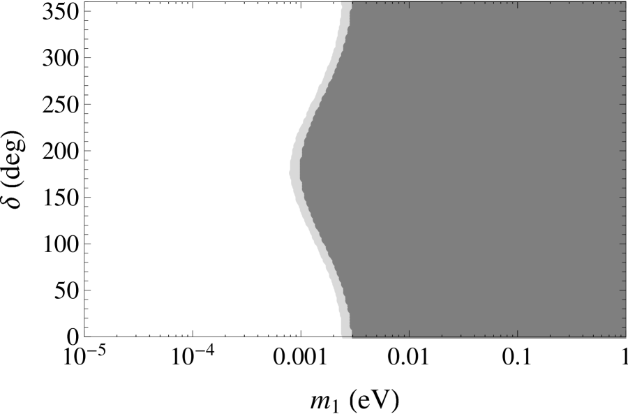
    MμμCμμ=detMsubscript𝑀𝜇𝜇subscript𝐶𝜇𝜇𝑀M_{\mu\mu}C_{\mu\mu}=\det M. This case is allowed for both hierarchies, and the allowed regions are shown in Fig. 5.

  3. 3.

    MττCττ=detMsubscript𝑀𝜏𝜏subscript𝐶𝜏𝜏𝑀M_{\tau\tau}C_{\tau\tau}=\det M. This case is allowed for both hierarchies, and the allowed regions are shown in Fig. 6. The allowed regions are similar to Fig. 5 with δδ+180𝛿𝛿superscript180\delta\rightarrow\delta+180^{\circ} for both hierarchies because of the approximate μτ𝜇𝜏\mu-\tau symmetry of the data.

Refer to caption
Refer to caption
Figure 5: The allowed regions for the constraint MμμCμμ=detMsubscript𝑀𝜇𝜇subscript𝐶𝜇𝜇𝑀M_{\mu\mu}C_{\mu\mu}=\det M. The left (right) panel is for the normal (inverted) hierarchy. The dark shaded regions correspond to the best-fit oscillation parameters, while the light shaded regions are allowed at 2σ2𝜎2\sigma.
Refer to caption
Refer to caption
Figure 6: Same as Fig. 5, except for MττCττ=detMsubscript𝑀𝜏𝜏subscript𝐶𝜏𝜏𝑀M_{\tau\tau}C_{\tau\tau}=\det M.

4.5 Class 7

With x=eiϕ2𝑥superscript𝑒𝑖subscriptitalic-ϕ2x=e^{-i\phi_{2}} and y=eiϕ3𝑦superscript𝑒𝑖subscriptitalic-ϕ3y=e^{-i\phi_{3}}, the constraint Mαα2Cαα=4MαβMαγCβγsuperscriptsubscript𝑀𝛼𝛼2subscript𝐶𝛼𝛼4subscript𝑀𝛼𝛽subscript𝑀𝛼𝛾subscript𝐶𝛽𝛾M_{\alpha\alpha}^{2}C_{\alpha\alpha}=4M_{\alpha\beta}M_{\alpha\gamma}C_{\beta\gamma} can be written as

ax3+bx2+cx+d=0,𝑎superscript𝑥3𝑏superscript𝑥2𝑐𝑥𝑑0ax^{3}+bx^{2}+cx+d=0\,, (32)

where

a=m22Uα22m1m3[(m1Uα32+m3Uα12y)Uα224(m1Uβ3Uγ3+m3Uβ1Uγ1y)Uβ2Uγ2],\displaystyle a=\frac{m_{2}^{2}U_{\alpha 2}^{*}{}^{2}}{m_{1}m_{3}}\left[(m_{1}U_{\alpha 3}^{2}+m_{3}U_{\alpha 1}^{2}y)U_{\alpha 2}^{*}{}^{2}-4(m_{1}U_{\beta 3}U_{\gamma 3}+m_{3}U_{\beta 1}U_{\gamma 1}y)U_{\beta 2}^{*}U_{\gamma 2}^{*}\right]\,, (33)
b𝑏\displaystyle b =m2Uα2m1m3{2m1(m1Uα32+m3Uα12y)Uα1Uα22\displaystyle=\frac{m_{2}U_{\alpha 2}^{*}}{m_{1}m_{3}}\left\{2m_{1}(m_{1}U_{\alpha 3}^{2}+m_{3}U_{\alpha 1}^{2}y)U_{\alpha 1}^{*}{}^{2}U_{\alpha 2}^{*}\right.
4m1(m1Uβ3Uγ3+m3Uβ1Uγ1y)Uα1(Uβ2Uγ1+Uβ1Uγ2)4subscript𝑚1subscript𝑚1subscript𝑈𝛽3subscript𝑈𝛾3subscript𝑚3subscript𝑈𝛽1subscript𝑈𝛾1𝑦superscriptsubscript𝑈𝛼1superscriptsubscript𝑈𝛽2superscriptsubscript𝑈𝛾1superscriptsubscript𝑈𝛽1superscriptsubscript𝑈𝛾2\displaystyle\left.-4m_{1}(m_{1}U_{\beta 3}U_{\gamma 3}+m_{3}U_{\beta 1}U_{\gamma 1}y)U_{\alpha 1}^{*}(U_{\beta 2}^{*}U_{\gamma 1}^{*}+U_{\beta 1}^{*}U_{\gamma 2}^{*})\right.
+m3y[m1Uα22Uα2+32Uα2(m1|Uα3|4+m3yUα12Uα322m1Uβ2Uγ2Uβ2Uγ2)\displaystyle\left.+m_{3}y\left[m_{1}U_{\alpha 2}^{2}U_{\alpha 2}^{*}{}^{3}+2U_{\alpha 2}^{*}(m_{1}|U_{\alpha 3}|^{4}+m_{3}yU_{\alpha 1}^{2}U_{\alpha 3}^{*}{}^{2}-2m_{1}U_{\beta 2}U_{\gamma 2}U_{\beta 2}^{*}U_{\gamma 2}^{*})\right.\right.
4(m1Uβ3Uγ3+m3yUβ1Uγ1)Uα3(Uβ3Uγ2+Uβ2Uγ3)]},\displaystyle\left.\left.-4(m_{1}U_{\beta 3}U_{\gamma 3}+m_{3}yU_{\beta 1}U_{\gamma 1})U_{\alpha 3}^{*}(U_{\beta 3}^{*}U_{\gamma 2}^{*}+U_{\beta 2}^{*}U_{\gamma 3}^{*})\right]\right\}\,, (34)
c𝑐\displaystyle c =1m1m3{m12(m1Uα32+m3Uα12y)Uα14\displaystyle=\frac{1}{m_{1}m_{3}}\left\{m_{1}^{2}(m_{1}U_{\alpha 3}^{2}+m_{3}U_{\alpha 1}^{2}y)U_{\alpha 1}^{*}{}^{4}\right.
+2m1Uα1[m3y(m1|Uα2|4+m1|Uα3|4+m3yUα12Uα3)22\displaystyle\left.+2m_{1}U_{\alpha 1}^{*}{}^{2}\left[m_{3}y(m_{1}|U_{\alpha 2}|^{4}+m_{1}|U_{\alpha 3}|^{4}+m_{3}yU_{\alpha 1}^{2}U_{\alpha 3}^{*}{}^{2})\right.\right.
2m1(m1Uβ3Uγ3+m3yUβ1Uγ1)Uβ1Uγ1]\displaystyle\left.\left.-2m_{1}(m_{1}U_{\beta 3}U_{\gamma 3}+m_{3}yU_{\beta 1}U_{\gamma 1})U_{\beta 1}^{*}U_{\gamma 1}^{*}\right]\right.
4m1m3yUα1[m1Uβ2Uγ2Uα2(Uβ2Uγ1+Uβ1Uγ2)\displaystyle-4m_{1}m_{3}yU_{\alpha 1}^{*}\left[m_{1}U_{\beta 2}U_{\gamma 2}U_{\alpha 2}^{*}(U_{\beta 2}^{*}U_{\gamma 1}^{*}+U_{\beta 1}^{*}U_{\gamma 2}^{*})\right.
+(m1Uβ3Uγ3+m3yUβ1Uγ1)Uα3(Uβ3Uγ1+Uβ1Uγ3)]\displaystyle\left.+(m_{1}U_{\beta 3}U_{\gamma 3}+m_{3}yU_{\beta 1}U_{\gamma 1})U_{\alpha 3}^{*}(U_{\beta 3}^{*}U_{\gamma 1}^{*}+U_{\beta 1}^{*}U_{\gamma 3}^{*})\right]
+m32y2Uα3[2m1|Uα2|4Uα34(m1Uβ3Uγ3+m3yUβ1Uγ1)Uα3Uβ3Uγ3\displaystyle\left.+m_{3}^{2}y^{2}U_{\alpha 3}^{*}\left[2m_{1}|U_{\alpha 2}|^{4}U_{\alpha 3}^{*}-4(m_{1}U_{\beta 3}U_{\gamma 3}+m_{3}yU_{\beta 1}U_{\gamma 1})U_{\alpha 3}^{*}U_{\beta 3}^{*}U_{\gamma 3}^{*}\right.\right.
+(m1Uα32+m3Uα12y)(Uα3)34m1Uβ2Uγ2Uα2(Uβ3Uγ2+Uβ2Uγ3)]},\displaystyle\left.\left.+(m_{1}U_{\alpha 3}^{2}+m_{3}U_{\alpha 1}^{2}y)(U_{\alpha 3}^{*})^{3}-4m_{1}U_{\beta 2}U_{\gamma 2}U_{\alpha 2}^{*}(U_{\beta 3}^{*}U_{\gamma 2}^{*}+U_{\beta 2}^{*}U_{\gamma 3}^{*})\right]\right\}\,, (35)
d𝑑\displaystyle d =ym2[m12Uα22Uα1+42m1Uα1(m3Uα22yUα322m1Uβ2Uγ2Uβ1Uγ1)2\displaystyle=\frac{y}{m_{2}}\left[m_{1}^{2}U_{\alpha 2}^{2}U_{\alpha 1}^{*}{}^{4}+2m_{1}U_{\alpha 1}^{*}{}^{2}(m_{3}U_{\alpha 2}^{2}yU_{\alpha 3}^{*}{}^{2}-2m_{1}U_{\beta 2}U_{\gamma 2}U_{\beta 1}^{*}U_{\gamma 1}^{*})\right.
4m1m3Uβ2Uγ2yUα1Uα3(Uβ3Uγ1+Uβ1Uγ3)+m32y2Uα3(Uα22Uα324Uβ2Uγ2Uβ3Uγ3)2].\displaystyle\left.-4m_{1}m_{3}U_{\beta 2}U_{\gamma 2}yU_{\alpha 1}^{*}U_{\alpha 3}^{*}(U_{\beta 3}^{*}U_{\gamma 1}^{*}+U_{\beta 1}^{*}U_{\gamma 3}^{*})+m_{3}^{2}y^{2}U_{\alpha 3}^{*}{}^{2}(U_{\alpha 2}^{2}U_{\alpha 3}^{*}{}^{2}-4U_{\beta 2}U_{\gamma 2}U_{\beta 3}^{*}U_{\gamma 3}^{*})\right]\,. (36)

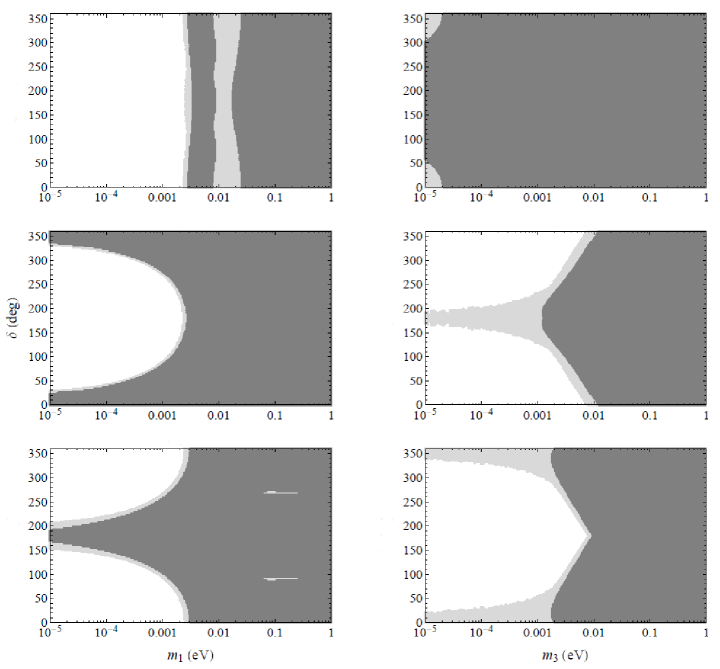
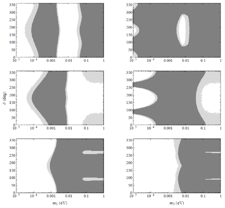
For a fixed set of δ𝛿\delta, m1subscript𝑚1m_{1} (m3subscript𝑚3m_{3}) for the NH (IH), and a given set of oscillation parameters, we solve the cubic equation (Eq. 32) to find x𝑥x as a function of y𝑦y, and then scan over ϕ3subscriptitalic-ϕ3\phi_{3} from 0 to 2π2𝜋2\pi to find where (if) |x|=1𝑥1|x|=1. If |x|=1𝑥1|x|=1 is found, there is a solution for ϕ2subscriptitalic-ϕ2\phi_{2} and ϕ3subscriptitalic-ϕ3\phi_{3}. By keeping the values of m1subscript𝑚1m_{1} (m3subscript𝑚3m_{3}) and δ𝛿\delta that have a solution, we obtain the allowed regions in the m1δsubscript𝑚1𝛿m_{1}-\delta (m3δsubscript𝑚3𝛿m_{3}-\delta) space for the NH (IH). All the cases in Class 7 are allowed for the both hierarchies, and the allowed regions are shown in Fig. 7. The 2σ𝜎\sigma allowed regions in the second row of Fig. 7 are similar to the third row of Fig. 7 with δδ+180𝛿𝛿superscript180\delta\rightarrow\delta+180^{\circ} for both hierarchies because of the approximate μτ𝜇𝜏\mu-\tau symmetry of the data.

Refer to caption
Figure 7: The first, second and third rows show the allowed regions for the constraints, Mee2Cee=4MeμMeτCμτsuperscriptsubscript𝑀𝑒𝑒2subscript𝐶𝑒𝑒4subscript𝑀𝑒𝜇subscript𝑀𝑒𝜏subscript𝐶𝜇𝜏M_{ee}^{2}C_{ee}=4M_{e\mu}M_{e\tau}C_{\mu\tau}, Mμμ2Cμμ=4MeμMμτCeτsuperscriptsubscript𝑀𝜇𝜇2subscript𝐶𝜇𝜇4subscript𝑀𝑒𝜇subscript𝑀𝜇𝜏subscript𝐶𝑒𝜏M_{\mu\mu}^{2}C_{\mu\mu}=4M_{e\mu}M_{\mu\tau}C_{e\tau} and Mττ2Cττ=4MeτMμτCeμsuperscriptsubscript𝑀𝜏𝜏2subscript𝐶𝜏𝜏4subscript𝑀𝑒𝜏subscript𝑀𝜇𝜏subscript𝐶𝑒𝜇M_{\tau\tau}^{2}C_{\tau\tau}=4M_{e\tau}M_{\mu\tau}C_{e\mu}, respectively. The dark shaded regions correspond to the best-fit oscillation parameters, while the light shaded regions are allowed at 2σ2𝜎2\sigma. The left (right) panels are for the normal (inverted) hierarchy.

4.6 Class 8

Since detM0𝑀0\det M\neq 0, the constraint MββdetM=Mαβ2Cααsubscript𝑀𝛽𝛽𝑀superscriptsubscript𝑀𝛼𝛽2subscript𝐶𝛼𝛼M_{\beta\beta}\det M=-M_{\alpha\beta}^{2}C_{\alpha\alpha} is equivalent to

Mββ=Mαβ2(M1)αα.subscript𝑀𝛽𝛽superscriptsubscript𝑀𝛼𝛽2subscriptsuperscript𝑀1𝛼𝛼M_{\beta\beta}=-M_{\alpha\beta}^{2}(M^{-1})_{\alpha\alpha}\,. (37)

Similar to Class 7, defining x=eiϕ2𝑥superscript𝑒𝑖subscriptitalic-ϕ2x=e^{-i\phi_{2}} and y=eiϕ3𝑦superscript𝑒𝑖subscriptitalic-ϕ3y=e^{-i\phi_{3}}, we can write the constraint as

ax3+bx2+cx+d=0,superscript𝑎superscript𝑥3superscript𝑏superscript𝑥2superscript𝑐𝑥superscript𝑑0a^{\prime}x^{3}+b^{\prime}x^{2}+c^{\prime}x+d^{\prime}=0\,, (38)

where

a=m22Uα2Uβ22(m1Uα32+m3yUα12)2m1m3,\displaystyle a^{\prime}=\frac{m_{2}^{2}U_{\text{$\alpha$2}}^{*}{}^{2}U_{\text{$\beta$2}}^{*}{}^{2}\left(m_{1}U_{\text{$\alpha$3}}^{2}+m_{3}yU_{\text{$\alpha$1}}^{2}\right)}{m_{1}m_{3}}\,, (39)
b=m2Uβ2[yUβ2(|Uα2|+41)+2Uα2(ym11Uα12+m31Uα32)(m1Uα1Uβ1+m3yUα3Uβ3)],\displaystyle b^{\prime}=m_{2}U_{\text{$\beta$2}}^{*}\left[yU_{\text{$\beta$2}}^{*}\left(\left|U_{\text{$\alpha$2}}\right|{}^{4}+1\right)+2U_{\text{$\alpha$2}}^{*}\left(ym_{1}^{-1}U_{\alpha 1}^{2}+m_{3}^{-1}U_{\alpha 3}^{2}\right)\left(m_{1}U_{\text{$\alpha$1}}^{*}U_{\text{$\beta$1}}^{*}+m_{3}yU_{\text{$\alpha$3}}^{*}U_{\text{$\beta$3}}^{*}\right)\right]\,, (40)
c=superscript𝑐absent\displaystyle c^{\prime}= y(m1Uβ1+2m3yUβ3)2+2yUα2Uβ2Uα22(m1Uα1Uβ1+m3yUα3Uβ3)\displaystyle y\left(m_{1}U_{\text{$\beta$1}}^{*}{}^{2}+m_{3}yU_{\text{$\beta$3}}^{*}{}^{2}\right)+2yU_{\text{$\alpha$2}}^{*}U_{\text{$\beta$2}}^{*}U_{\text{$\alpha$2}}^{2}\left(m_{1}U_{\text{$\alpha$1}}^{*}U_{\text{$\beta$1}}^{*}+m_{3}yU_{\text{$\alpha$3}}^{*}U_{\text{$\beta$3}}^{*}\right) (41)
+(m1Uα1Uβ1+m3yUα3Uβ3)2(ym11Uα12+m31Uα32),superscriptsubscript𝑚1superscriptsubscript𝑈α1superscriptsubscript𝑈β1subscript𝑚3𝑦superscriptsubscript𝑈α3superscriptsubscript𝑈β32𝑦superscriptsubscript𝑚11superscriptsubscript𝑈𝛼12superscriptsubscript𝑚31superscriptsubscript𝑈𝛼32\displaystyle+\left(m_{1}U_{\text{$\alpha$1}}^{*}U_{\text{$\beta$1}}^{*}+m_{3}yU_{\text{$\alpha$3}}^{*}U_{\text{$\beta$3}}^{*}\right)^{2}\left(ym_{1}^{-1}U_{\alpha 1}^{2}+m_{3}^{-1}U_{\alpha 3}^{2}\right)\,,
d=yUα22(m1Uα1Uβ1+m3Uα3Uβ3y)2m2.\displaystyle d^{\prime}=\frac{yU_{\text{$\alpha$2}}^{2}\left(m_{1}U_{\text{$\alpha$1}}^{*}U_{\text{$\beta$1}}^{*}+m_{3}U_{\text{$\alpha$3}}^{*}U_{\text{$\beta$3}}^{*}y\right){}^{2}}{m_{2}}\,. (42)

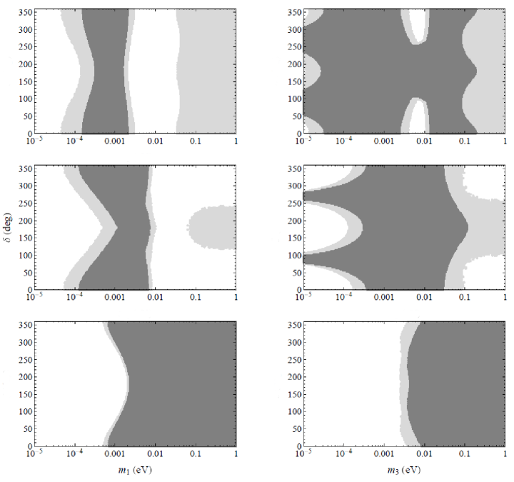
The solutions for ϕ2subscriptitalic-ϕ2\phi_{2} and ϕ3subscriptitalic-ϕ3\phi_{3} then proceed as in Class 7. We find all the cases in Class 8 are allowed for the both hierarchies and the allowed regions are shown in Figs. 8 and 9. Due to the approximate μτ𝜇𝜏\mu-\tau symmetry in the experimental data, the 2σ𝜎\sigma allowed regions in each row of Fig. 8 are similar to those in the corresponding row of Fig. 9 with δδ+180𝛿𝛿superscript180\delta\rightarrow\delta+180^{\circ} for both hierarchies.

Refer to caption
Figure 8: Same as Fig. 7, except that the first, second and third rows show the results for the constraints, MμμdetM=Meμ2Ceesubscript𝑀𝜇𝜇𝑀superscriptsubscript𝑀𝑒𝜇2subscript𝐶𝑒𝑒M_{\mu\mu}\det M=-M_{e\mu}^{2}C_{ee}, MeedetM=Meμ2Cμμsubscript𝑀𝑒𝑒𝑀superscriptsubscript𝑀𝑒𝜇2subscript𝐶𝜇𝜇M_{ee}\det M=-M_{e\mu}^{2}C_{\mu\mu} and MττdetM=Mμτ2Cμμsubscript𝑀𝜏𝜏𝑀superscriptsubscript𝑀𝜇𝜏2subscript𝐶𝜇𝜇M_{\tau\tau}\det M=-M_{\mu\tau}^{2}C_{\mu\mu}, respectively.
Refer to caption
Figure 9: Same as Fig. 7, except that the first, second and third rows show the results for the constraints, MττdetM=Meτ2Ceesubscript𝑀𝜏𝜏𝑀superscriptsubscript𝑀𝑒𝜏2subscript𝐶𝑒𝑒M_{\tau\tau}\det M=-M_{e\tau}^{2}C_{ee}, MeedetM=Meτ2Cττsubscript𝑀𝑒𝑒𝑀superscriptsubscript𝑀𝑒𝜏2subscript𝐶𝜏𝜏M_{ee}\det M=-M_{e\tau}^{2}C_{\tau\tau} and MμμdetM=Mμτ2Cττsubscript𝑀𝜇𝜇𝑀superscriptsubscript𝑀𝜇𝜏2subscript𝐶𝜏𝜏M_{\mu\mu}\det M=-M_{\mu\tau}^{2}C_{\tau\tau}, respectively.

5 Discussion and conclusion

We carried out a systematic study of zeros in the Dirac and RH Majorana neutrino mass matrices in the context of the Type I seesaw mechanism. We derived complex constraints on the light neutrino mass matrix for various textures in both the Dirac and RH Majorana neutrino mass matrices. There are 9 nonstandard constraints besides the standard ones that can be expressed in the form of one or two element/cofactor zeros alone. We showed that both the standard and nonstandard constraints are stable under one-loop RGE running from the lightest RH neutrino mass scale M1subscript𝑀1M_{1} to the electroweak scale MZsubscript𝑀𝑍M_{Z}. In addition, we studied the phenomenological implications for the nonstandard constraints, and found that some cases for the normal or inverted hierarchy are excluded, and for the rest we obtain the allowed regions for the lightest mass and Dirac CP phase, which will be probed in the next generation of neutrino experiments. We found 12 new models (Classes 6, 7 and 8) not previously discussed in the literature which are allowed at 2σ2𝜎2\sigma for both the normal and inverted hierarchies.

Once the lightest neutrino mass and Dirac CP phase are determined, the rate for neutrinoless double beta decay (0νββ0𝜈𝛽𝛽0\nu\beta\beta), which depends on the magnitude of the νeνesubscript𝜈𝑒subscript𝜈𝑒\nu_{e}-\nu_{e} element of the neutrino mass matrix,

|Mee|=|m1c122c132+m2eiϕ2s122c132+m3eiϕ3s132e2iδ|,subscript𝑀𝑒𝑒subscript𝑚1superscriptsubscript𝑐122superscriptsubscript𝑐132subscript𝑚2superscript𝑒𝑖subscriptitalic-ϕ2superscriptsubscript𝑠122superscriptsubscript𝑐132subscript𝑚3superscript𝑒𝑖subscriptitalic-ϕ3superscriptsubscript𝑠132superscript𝑒2𝑖𝛿|M_{ee}|=|m_{1}c_{12}^{2}c_{13}^{2}+m_{2}e^{-i\phi_{2}}s_{12}^{2}c_{13}^{2}+m_{3}e^{-i\phi_{3}}s_{13}^{2}e^{2i\delta}|\,, (43)

is fixed.

In Table 2, we list the minimum and maximum values of |Mee|subscript𝑀𝑒𝑒|M_{ee}| at the 2σ2𝜎2\sigma level for Class 2, 3, 4 and 5 constraints. In Table 3, we list the minimum values for Class 6, 7, 8 and 9 constraints with the best-fit oscillation parameters and the 2σ2𝜎2\sigma lower bounds. The maximum values for Class 6, 7, 8 and 9 constraints are all above 1000 meV. The most stringent experimental upper limit on the effective mass |Mee|subscript𝑀𝑒𝑒|M_{ee}| is 120250120250120-250 meV at 90% C.L. [23]. Some cases in Class 3, 4 and 5 could be ruled out once the sensitivities to |Mee|subscript𝑀𝑒𝑒|M_{ee}| reach about 50 meV for the currently running 0νββ0𝜈𝛽𝛽0\nu\beta\beta experiments [24]. Nevertheless, the minimum values of |Mee|subscript𝑀𝑒𝑒|M_{ee}| for Class 6, 7, 8 and 9 constraints are all below 505050 meV and can be completely probed only if the sensitivity of future 0νββ0𝜈𝛽𝛽0\nu\beta\beta experiments is significantly improved. Note that the minimum value of |Mee|subscript𝑀𝑒𝑒|M_{ee}| is about 15 meV for the IH and 0 for the NH. The mass hierarchy will also be determined if |Mee|subscript𝑀𝑒𝑒|M_{ee}| can be pushed to 15 meV in the future.

Recent global fits [21, 25, 26] indicate a slight preference for a nonzero Dirac CP phase, with a preferred value δ270similar-to𝛿superscript270\delta\sim 270^{\circ}. Also, combined T2K and reactor analyses show a weak hint for the normal hierarchy [27]. Most viable cases of the nonstandard constraints allow δ=270𝛿superscript270\delta=270^{\circ}, except for two cases in Class 5: Cee=0subscript𝐶𝑒𝑒0C_{ee}=0, CμμCeτ=2CeμCμτsubscript𝐶𝜇𝜇subscript𝐶𝑒𝜏2subscript𝐶𝑒𝜇subscript𝐶𝜇𝜏C_{\mu\mu}C_{e\tau}=2C_{e\mu}C_{\mu\tau} and Cee=0subscript𝐶𝑒𝑒0C_{ee}=0, CττCeμ=2CeτCμτsubscript𝐶𝜏𝜏subscript𝐶𝑒𝜇2subscript𝐶𝑒𝜏subscript𝐶𝜇𝜏C_{\tau\tau}C_{e\mu}=2C_{e\tau}C_{\mu\tau}. These two cases may be ruled out if future measurements find δ𝛿\delta to be close to 270superscript270270^{\circ}. If the hint for the normal hierarchy is confirmed, Classes 2 and 3, and the IH cases in the other classes will be ruled out.

Class Constraints Hierarchy Minimum Maximum
2 Mμμ=0subscript𝑀𝜇𝜇0M_{\mu\mu}=0 and detM=0𝑀0\det M=0 IH 15 18
2 Mττ=0subscript𝑀𝜏𝜏0M_{\tau\tau}=0 and detM=0𝑀0\det M=0 IH 15 17
3 Meμ=0subscript𝑀𝑒𝜇0M_{e\mu}=0 and detM=0𝑀0\det M=0 IH 46 48
3 Meτ=0subscript𝑀𝑒𝜏0M_{e\tau}=0 and detM=0𝑀0\det M=0 IH 46 48
4 Mμμ=0subscript𝑀𝜇𝜇0M_{\mu\mu}=0 and MττMeμ=2MμτMeτsubscript𝑀𝜏𝜏subscript𝑀𝑒𝜇2subscript𝑀𝜇𝜏subscript𝑀𝑒𝜏M_{\tau\tau}M_{e\mu}=2M_{\mu\tau}M_{e\tau} NH 41 278
4 Mμμ=0subscript𝑀𝜇𝜇0M_{\mu\mu}=0 and MττMeμ=2MμτMeτsubscript𝑀𝜏𝜏subscript𝑀𝑒𝜇2subscript𝑀𝜇𝜏subscript𝑀𝑒𝜏M_{\tau\tau}M_{e\mu}=2M_{\mu\tau}M_{e\tau} IH 16 214
4 Mττ=0subscript𝑀𝜏𝜏0M_{\tau\tau}=0 and MμμMeτ=2MμτMeμsubscript𝑀𝜇𝜇subscript𝑀𝑒𝜏2subscript𝑀𝜇𝜏subscript𝑀𝑒𝜇M_{\mu\mu}M_{e\tau}=2M_{\mu\tau}M_{e\mu} NH 65 277
4 Mττ=0subscript𝑀𝜏𝜏0M_{\tau\tau}=0 and MμμMeτ=2MμτMeμsubscript𝑀𝜇𝜇subscript𝑀𝑒𝜏2subscript𝑀𝜇𝜏subscript𝑀𝑒𝜇M_{\mu\mu}M_{e\tau}=2M_{\mu\tau}M_{e\mu} IH 15 223
5 Cee=0subscript𝐶𝑒𝑒0C_{ee}=0 and CμμCeτ=2CeμCμτsubscript𝐶𝜇𝜇subscript𝐶𝑒𝜏2subscript𝐶𝑒𝜇subscript𝐶𝜇𝜏C_{\mu\mu}C_{e\tau}=2C_{e\mu}C_{\mu\tau} IH 19 23
5 Cee=0subscript𝐶𝑒𝑒0C_{ee}=0 and CττCeμ=2CeτCμτsubscript𝐶𝜏𝜏subscript𝐶𝑒𝜇2subscript𝐶𝑒𝜏subscript𝐶𝜇𝜏C_{\tau\tau}C_{e\mu}=2C_{e\tau}C_{\mu\tau} IH 19 24
5 Cμμ=0subscript𝐶𝜇𝜇0C_{\mu\mu}=0 and CττCeμ=2CμτCeτsubscript𝐶𝜏𝜏subscript𝐶𝑒𝜇2subscript𝐶𝜇𝜏subscript𝐶𝑒𝜏C_{\tau\tau}C_{e\mu}=2C_{\mu\tau}C_{e\tau} NH 64 278
5 Cμμ=0subscript𝐶𝜇𝜇0C_{\mu\mu}=0 and CττCeμ=2CμτCeτsubscript𝐶𝜏𝜏subscript𝐶𝑒𝜇2subscript𝐶𝜇𝜏subscript𝐶𝑒𝜏C_{\tau\tau}C_{e\mu}=2C_{\mu\tau}C_{e\tau} IH 65 222
5 Cττ=0subscript𝐶𝜏𝜏0C_{\tau\tau}=0 and CμμCeτ=2CμτCeμsubscript𝐶𝜇𝜇subscript𝐶𝑒𝜏2subscript𝐶𝜇𝜏subscript𝐶𝑒𝜇C_{\mu\mu}C_{e\tau}=2C_{\mu\tau}C_{e\mu} NH 39 268
5 Cττ=0subscript𝐶𝜏𝜏0C_{\tau\tau}=0 and CμμCeτ=2CμτCeμsubscript𝐶𝜇𝜇subscript𝐶𝑒𝜏2subscript𝐶𝜇𝜏subscript𝐶𝑒𝜇C_{\mu\mu}C_{e\tau}=2C_{\mu\tau}C_{e\mu} IH 61 219
Table 2: The minimum and maximum values of |Mee|subscript𝑀𝑒𝑒|M_{ee}| (in meV) for Class 2, 3, 4 and 5 constraints at 2σ2𝜎2\sigma.
Class Constraints Best-fit 2σ2𝜎2\sigma lower bound
NH IH NH IH
6 MeeCee=detMsubscript𝑀𝑒𝑒subscript𝐶𝑒𝑒𝑀M_{ee}C_{ee}=\det M 3.2 17.9 2.6 15.1
6 MμμCμμ=detMsubscript𝑀𝜇𝜇subscript𝐶𝜇𝜇𝑀M_{\mu\mu}C_{\mu\mu}=\det M 0.2 17.9 0.0 14.9
6 MττCττ=detMsubscript𝑀𝜏𝜏subscript𝐶𝜏𝜏𝑀M_{\tau\tau}C_{\tau\tau}=\det M 0.8 17.9 0.0 15.0
7 Mee2Cee=4MeμMeτCμτsuperscriptsubscript𝑀𝑒𝑒2subscript𝐶𝑒𝑒4subscript𝑀𝑒𝜇subscript𝑀𝑒𝜏subscript𝐶𝜇𝜏M_{ee}^{2}C_{ee}=4M_{e\mu}M_{e\tau}C_{\mu\tau} 0.0 41.4 0.0 39.6
7 Mμμ2Cμμ=4MμτMeμCeτsuperscriptsubscript𝑀𝜇𝜇2subscript𝐶𝜇𝜇4subscript𝑀𝜇𝜏subscript𝑀𝑒𝜇subscript𝐶𝑒𝜏M_{\mu\mu}^{2}C_{\mu\mu}=4M_{\mu\tau}M_{e\mu}C_{e\tau} 0.9 17.9 0.6 15.0
7 Mττ2Cττ=4MeτMμτCeμsuperscriptsubscript𝑀𝜏𝜏2subscript𝐶𝜏𝜏4subscript𝑀𝑒𝜏subscript𝑀𝜇𝜏subscript𝐶𝑒𝜇M_{\tau\tau}^{2}C_{\tau\tau}=4M_{e\tau}M_{\mu\tau}C_{e\mu} 0.8 17.9 0.5 15.0
8 MμμdetM=Meμ2Ceesubscript𝑀𝜇𝜇𝑀superscriptsubscript𝑀𝑒𝜇2subscript𝐶𝑒𝑒M_{\mu\mu}\det M=-M_{e\mu}^{2}C_{ee} 1.6 18.0 1.3 14.9
8 MττdetM=Meτ2Ceesubscript𝑀𝜏𝜏𝑀superscriptsubscript𝑀𝑒𝜏2subscript𝐶𝑒𝑒M_{\tau\tau}\det M=-M_{e\tau}^{2}C_{ee} 1.7 17.9 1.4 14.9
8 MeedetM=Meμ2Cμμsubscript𝑀𝑒𝑒𝑀superscriptsubscript𝑀𝑒𝜇2subscript𝐶𝜇𝜇M_{ee}\det M=-M_{e\mu}^{2}C_{\mu\mu} 0.0 21.7 0.0 18.1
8 MττdetM=Mμτ2Cμμsubscript𝑀𝜏𝜏𝑀superscriptsubscript𝑀𝜇𝜏2subscript𝐶𝜇𝜇M_{\tau\tau}\det M=-M_{\mu\tau}^{2}C_{\mu\mu} 0.5 17.9 0.2 15.0
8 MeedetM=Meτ2Cττsubscript𝑀𝑒𝑒𝑀superscriptsubscript𝑀𝑒𝜏2subscript𝐶𝜏𝜏M_{ee}\det M=-M_{e\tau}^{2}C_{\tau\tau} 0.0 20.3 0.0 18.6
8 MμμdetM=Mμτ2Cττsubscript𝑀𝜇𝜇𝑀superscriptsubscript𝑀𝜇𝜏2subscript𝐶𝜏𝜏M_{\mu\mu}\det M=-M_{\mu\tau}^{2}C_{\tau\tau} 0.5 17.9 0.2 15.0
9 detM=0𝑀0\det M=0 1.4 17.9 1.2 14.8
Table 3: The minimum values of |Mee|subscript𝑀𝑒𝑒|M_{ee}| (in meV) for Class 6, 7, 8 and 9 constraints for the best-fit oscillation parameters, and the 2σ2𝜎2\sigma lower bounds.

Acknowledgements. This research was supported by the DOE under grant No. DE-SC0010504 and by the Kavli Institute for Theoretical Physics under NSF grant No. PHY11-25915.

Appendix A Textures for the nonstandard constraints

We list all possible structures that lead to the nonstandard constraints for N=NR+ND7𝑁subscript𝑁𝑅subscript𝑁𝐷7N=N_{R}+N_{D}\geq 7. Also we do not consider ND7subscript𝑁𝐷7N_{D}\geq 7 because it has one row of zeros in MDsubscript𝑀𝐷M_{D}, which leads to three zeros in M𝑀M, which is excluded by experimental data. Following Ref. [9], we define Class X constraints on M𝑀M or Cdet(M)M1𝐶𝑀superscript𝑀1C\equiv\det(M)M^{-1} as one zero on diagonal and one off-diagonal zero sharing column and row, Class Y constraints as one zero on diagonal and one off-diagonal zero not sharing column and row, and Class Z constraints as two zeros on diagonal.

A.1 𝑵𝑹=𝟒subscript𝑵𝑹4\bm{N_{R}=4}

For NR=4subscript𝑁𝑅4N_{R}=4, there is only one structure for MRsubscript𝑀𝑅M_{R},

MR=[×0000×0×0],subscript𝑀𝑅matrix000000\displaystyle M_{R}=\begin{bmatrix}\times&0&0\\ 0&0&\times\\ 0&\times&0\end{bmatrix}\,, (44)

where the symbol ×\times denotes a nonzero matrix element. All other structures of MRsubscript𝑀𝑅M_{R} can be obtained by a permutation of the columns and rows of the above structure. If MDsubscript𝑀𝐷M_{D} has more than 5 zeros, M𝑀M or C𝐶C would have at least three zeros, so here we only consider ND5subscript𝑁𝐷5N_{D}\leq 5.

  1. 1.

    𝑵𝑫=𝟓subscript𝑵𝑫5\bm{N_{D}=5}. Of the 126 different structures of MDsubscript𝑀𝐷M_{D} in this case, 120 lead to at least three zeros in M𝑀M or C𝐶C, and only 6 structures lead to Class 1 nonstandard constraints. The 6 structures are:

    MD=[0×000×0××],[00×0×00××],subscript𝑀𝐷matrix00000matrix00000\displaystyle M_{D}=\begin{bmatrix}0&\times&0\\ 0&0&\times\\ 0&\times&\times\end{bmatrix}\,,\quad\quad\begin{bmatrix}0&0&\times\\ 0&\times&0\\ 0&\times&\times\end{bmatrix}\,, (45)

    which lead to the constraints, Mee=Mμμ=0subscript𝑀𝑒𝑒subscript𝑀𝜇𝜇0M_{ee}=M_{\mu\mu}=0 and detM=0𝑀0\det M=0;

    MD=[0×00××00×],[00×0××0×0],subscript𝑀𝐷matrix00000matrix00000\displaystyle M_{D}=\begin{bmatrix}0&\times&0\\ 0&\times&\times\\ 0&0&\times\end{bmatrix}\,,\quad\quad\begin{bmatrix}0&0&\times\\ 0&\times&\times\\ 0&\times&0\end{bmatrix}\,, (46)

    which lead to the constraints, Mee=Mττ=0subscript𝑀𝑒𝑒subscript𝑀𝜏𝜏0M_{ee}=M_{\tau\tau}=0 and detM=0𝑀0\det M=0;

    MD=[0××0×000×],[0××00×0×0],subscript𝑀𝐷matrix00000matrix00000\displaystyle M_{D}=\begin{bmatrix}0&\times&\times\\ 0&\times&0\\ 0&0&\times\end{bmatrix}\,,\quad\quad\begin{bmatrix}0&\times&\times\\ 0&0&\times\\ 0&\times&0\end{bmatrix}\,, (47)

    which lead to the constraints, Mμμ=Mττ=0subscript𝑀𝜇𝜇subscript𝑀𝜏𝜏0M_{\mu\mu}=M_{\tau\tau}=0 and detM=0𝑀0\det M=0.

  2. 2.

    𝑵𝑫=𝟒subscript𝑵𝑫4\bm{N_{D}=4}. Of the 126 different structures of MDsubscript𝑀𝐷M_{D} in this case, 39 lead to at least three zeros in M𝑀M or C𝐶C, 3 lead to a block diagonal matrix for M𝑀M, 36 lead to Class X constraints on M𝑀M, 6 lead to Class Z constraints on M𝑀M, 6 lead to Class Z constraints on C𝐶C, and 18 lead to one zero in M𝑀M and one zero in C𝐶C. In addition, there are 6 structures of MDsubscript𝑀𝐷M_{D} that lead to Class 2 nonstandard constraints:

    MD=[0×00××0××],[00×0××0××],subscript𝑀𝐷matrix0000matrix0000\displaystyle M_{D}=\begin{bmatrix}0&\times&0\\ 0&\times&\times\\ 0&\times&\times\end{bmatrix}\,,\quad\quad\begin{bmatrix}0&0&\times\\ 0&\times&\times\\ 0&\times&\times\end{bmatrix}\,, (48)

    which lead to the constraints, Mee=0subscript𝑀𝑒𝑒0M_{ee}=0 and detM=0𝑀0\det M=0;

    MD=[0××0×00××],[0××00×0××],subscript𝑀𝐷matrix0000matrix0000\displaystyle M_{D}=\begin{bmatrix}0&\times&\times\\ 0&\times&0\\ 0&\times&\times\end{bmatrix}\,,\quad\quad\begin{bmatrix}0&\times&\times\\ 0&0&\times\\ 0&\times&\times\end{bmatrix}\,, (49)

    which lead to the constraints, Mμμ=0subscript𝑀𝜇𝜇0M_{\mu\mu}=0 and detM=0𝑀0\det M=0;

    MD=[0××0××0×0],[0××0××00×],subscript𝑀𝐷matrix0000matrix0000\displaystyle M_{D}=\begin{bmatrix}0&\times&\times\\ 0&\times&\times\\ 0&\times&0\end{bmatrix}\,,\quad\quad\begin{bmatrix}0&\times&\times\\ 0&\times&\times\\ 0&0&\times\end{bmatrix}\,, (50)

    which lead to the constraints, Mττ=0subscript𝑀𝜏𝜏0M_{\tau\tau}=0 and detM=0𝑀0\det M=0.

    The remaining 12 structures lead to Class 4 nonstandard constraints:

    MD=[0×00×××0×],[00×0××××0],subscript𝑀𝐷matrix0000matrix0000\displaystyle M_{D}=\begin{bmatrix}0&\times&0\\ 0&\times&\times\\ \times&0&\times\end{bmatrix}\,,\quad\quad\begin{bmatrix}0&0&\times\\ 0&\times&\times\\ \times&\times&0\end{bmatrix}\,, (51)

    which lead to the constraints, Mee=0subscript𝑀𝑒𝑒0M_{ee}=0 and MμμMeτ=2MeμMμτsubscript𝑀𝜇𝜇subscript𝑀𝑒𝜏2subscript𝑀𝑒𝜇subscript𝑀𝜇𝜏M_{\mu\mu}M_{e\tau}=2M_{e\mu}M_{\mu\tau};

    MD=[0×0×0×0××],[00×××00××],subscript𝑀𝐷matrix0000matrix0000\displaystyle M_{D}=\begin{bmatrix}0&\times&0\\ \times&0&\times\\ 0&\times&\times\end{bmatrix}\,,\quad\quad\begin{bmatrix}0&0&\times\\ \times&\times&0\\ 0&\times&\times\end{bmatrix}\,, (52)

    which lead to the constraints, Mee=0subscript𝑀𝑒𝑒0M_{ee}=0 and MττMeμ=2MeτMμτsubscript𝑀𝜏𝜏subscript𝑀𝑒𝜇2subscript𝑀𝑒𝜏subscript𝑀𝜇𝜏M_{\tau\tau}M_{e\mu}=2M_{e\tau}M_{\mu\tau};

    MD=[0××0×0×0×],[0××00×××0],subscript𝑀𝐷matrix0000matrix0000\displaystyle M_{D}=\begin{bmatrix}0&\times&\times\\ 0&\times&0\\ \times&0&\times\end{bmatrix}\,,\quad\quad\begin{bmatrix}0&\times&\times\\ 0&0&\times\\ \times&\times&0\end{bmatrix}\,, (53)

    which lead to the constraints, Mμμ=0subscript𝑀𝜇𝜇0M_{\mu\mu}=0 and MeeMμτ=2MeμMeτsubscript𝑀𝑒𝑒subscript𝑀𝜇𝜏2subscript𝑀𝑒𝜇subscript𝑀𝑒𝜏M_{ee}M_{\mu\tau}=2M_{e\mu}M_{e\tau};

    MD=[×0×0×00××],[××000×0××],subscript𝑀𝐷matrix0000matrix0000\displaystyle M_{D}=\begin{bmatrix}\times&0&\times\\ 0&\times&0\\ 0&\times&\times\end{bmatrix}\,,\quad\quad\begin{bmatrix}\times&\times&0\\ 0&0&\times\\ 0&\times&\times\end{bmatrix}\,, (54)

    which lead to the constraints, Mμμ=0subscript𝑀𝜇𝜇0M_{\mu\mu}=0 and MττMeμ=2MμτMeτsubscript𝑀𝜏𝜏subscript𝑀𝑒𝜇2subscript𝑀𝜇𝜏subscript𝑀𝑒𝜏M_{\tau\tau}M_{e\mu}=2M_{\mu\tau}M_{e\tau};

    MD=[×0×0××0×0],[××00××00×],subscript𝑀𝐷matrix0000matrix0000\displaystyle M_{D}=\begin{bmatrix}\times&0&\times\\ 0&\times&\times\\ 0&\times&0\end{bmatrix}\,,\quad\quad\begin{bmatrix}\times&\times&0\\ 0&\times&\times\\ 0&0&\times\end{bmatrix}\,, (55)

    which lead to the constraints, Mττ=0subscript𝑀𝜏𝜏0M_{\tau\tau}=0 and MμμMeτ=2MeμMμτsubscript𝑀𝜇𝜇subscript𝑀𝑒𝜏2subscript𝑀𝑒𝜇subscript𝑀𝜇𝜏M_{\mu\mu}M_{e\tau}=2M_{e\mu}M_{\mu\tau};

    MD=[0×××0×0×0],[0××××000×],subscript𝑀𝐷matrix0000matrix0000\displaystyle M_{D}=\begin{bmatrix}0&\times&\times\\ \times&0&\times\\ 0&\times&0\end{bmatrix}\,,\quad\quad\begin{bmatrix}0&\times&\times\\ \times&\times&0\\ 0&0&\times\end{bmatrix}\,, (56)

    which lead to the constraints, Mττ=0subscript𝑀𝜏𝜏0M_{\tau\tau}=0 and MeeMμτ=2MeμMeτsubscript𝑀𝑒𝑒subscript𝑀𝜇𝜏2subscript𝑀𝑒𝜇subscript𝑀𝑒𝜏M_{ee}M_{\mu\tau}=2M_{e\mu}M_{e\tau}.

  3. 3.

    𝑵𝑫=𝟑subscript𝑵𝑫3\bm{N_{D}=3}. Of the 84 different structures of MDsubscript𝑀𝐷M_{D} in this case, 5 lead to at least three zeros in M𝑀M or C𝐶C, 12 lead to Class X constraints on M𝑀M, 24 lead to one diagonal zero in M𝑀M, 6 lead to one off-diagonal zero in M𝑀M and 24 lead to one diagonal zero in C𝐶C. In addition, there are 6 structures that lead to Class 6 nonstandard constraints:

    MD=[××00××0××],[×0×0××0××],subscript𝑀𝐷matrix000matrix000\displaystyle M_{D}=\begin{bmatrix}\times&\times&0\\ 0&\times&\times\\ 0&\times&\times\end{bmatrix}\,,\quad\quad\begin{bmatrix}\times&0&\times\\ 0&\times&\times\\ 0&\times&\times\end{bmatrix}\,, (57)

    which lead to the constraint, MeeCee=detMsubscript𝑀𝑒𝑒subscript𝐶𝑒𝑒𝑀M_{ee}C_{ee}=\det M;

    MD=[0××××00××],[0×××0×0××],subscript𝑀𝐷matrix000matrix000\displaystyle M_{D}=\begin{bmatrix}0&\times&\times\\ \times&\times&0\\ 0&\times&\times\end{bmatrix}\,,\quad\quad\begin{bmatrix}0&\times&\times\\ \times&0&\times\\ 0&\times&\times\end{bmatrix}\,, (58)

    which lead to the constraint, MμμCμμ=detMsubscript𝑀𝜇𝜇subscript𝐶𝜇𝜇𝑀M_{\mu\mu}C_{\mu\mu}=\det M;

    MD=[0××0××××0],[0××0×××0×],subscript𝑀𝐷matrix000matrix000\displaystyle M_{D}=\begin{bmatrix}0&\times&\times\\ 0&\times&\times\\ \times&\times&0\end{bmatrix}\,,\quad\quad\begin{bmatrix}0&\times&\times\\ 0&\times&\times\\ \times&0&\times\end{bmatrix}\,, (59)

    which lead to the constraint, MττCττ=detMsubscript𝑀𝜏𝜏subscript𝐶𝜏𝜏𝑀M_{\tau\tau}C_{\tau\tau}=\det M.

    Also, there are 6 structures lead to Class 7 nonstandard constraints:

    MD=[0××××0×0×],[0×××0×××0],subscript𝑀𝐷matrix000matrix000\displaystyle M_{D}=\begin{bmatrix}0&\times&\times\\ \times&\times&0\\ \times&0&\times\end{bmatrix}\,,\quad\quad\begin{bmatrix}0&\times&\times\\ \times&0&\times\\ \times&\times&0\end{bmatrix}\,, (60)

    which lead to the constraint, Mee2Cee=4MeμMeτCμτsuperscriptsubscript𝑀𝑒𝑒2subscript𝐶𝑒𝑒4subscript𝑀𝑒𝜇subscript𝑀𝑒𝜏subscript𝐶𝜇𝜏M_{ee}^{2}C_{ee}=4M_{e\mu}M_{e\tau}C_{\mu\tau};

    MD=[××00×××0×],[×0×0××××0],subscript𝑀𝐷matrix000matrix000\displaystyle M_{D}=\begin{bmatrix}\times&\times&0\\ 0&\times&\times\\ \times&0&\times\end{bmatrix}\,,\quad\quad\begin{bmatrix}\times&0&\times\\ 0&\times&\times\\ \times&\times&0\end{bmatrix}\,, (61)

    which lead to the constraint, Mμμ2Cμμ=4MeμMμτCeτsuperscriptsubscript𝑀𝜇𝜇2subscript𝐶𝜇𝜇4subscript𝑀𝑒𝜇subscript𝑀𝜇𝜏subscript𝐶𝑒𝜏M_{\mu\mu}^{2}C_{\mu\mu}=4M_{e\mu}M_{\mu\tau}C_{e\tau};

    MD=[××0×0×0××],[×0×××00××],subscript𝑀𝐷matrix000matrix000\displaystyle M_{D}=\begin{bmatrix}\times&\times&0\\ \times&0&\times\\ 0&\times&\times\end{bmatrix}\,,\quad\quad\begin{bmatrix}\times&0&\times\\ \times&\times&0\\ 0&\times&\times\end{bmatrix}\,, (62)

    which lead to the constraint, Mττ2Cττ=4MeτMμτCeμsuperscriptsubscript𝑀𝜏𝜏2subscript𝐶𝜏𝜏4subscript𝑀𝑒𝜏subscript𝑀𝜇𝜏subscript𝐶𝑒𝜇M_{\tau\tau}^{2}C_{\tau\tau}=4M_{e\tau}M_{\mu\tau}C_{e\mu}.

    The remaining one structure leads to the Class 9 constraint, detM=0𝑀0\det M=0:

    MD=[0××0××0××].subscript𝑀𝐷matrix000\displaystyle M_{D}=\begin{bmatrix}0&\times&\times\\ 0&\times&\times\\ 0&\times&\times\end{bmatrix}\,. (63)

A.2 𝑵𝑹=𝟑subscript𝑵𝑹3\bm{N_{R}=3}

For NR=3subscript𝑁𝑅3N_{R}=3, there are four structures of MRsubscript𝑀𝑅M_{R} that are not equivalent under permutation. They are

MR1=[×000××0×0],MR2=[×0×00×××0],formulae-sequencesubscript𝑀𝑅1matrix00000subscript𝑀𝑅2matrix0000\displaystyle M_{R1}=\begin{bmatrix}\times&0&0\\ 0&\times&\times\\ 0&\times&0\end{bmatrix}\,,\quad M_{R2}=\begin{bmatrix}\times&0&\times\\ 0&0&\times\\ \times&\times&0\end{bmatrix}\,,
MR3=[0×××0×××0],MR4=[×000×000×].formulae-sequencesubscript𝑀𝑅3matrix000subscript𝑀𝑅4matrix000000\displaystyle M_{R3}=\begin{bmatrix}0&\times&\times\\ \times&0&\times\\ \times&\times&0\end{bmatrix}\,,\quad M_{R4}=\begin{bmatrix}\times&0&0\\ 0&\times&0\\ 0&0&\times\end{bmatrix}\,. (64)

All other structures of MRsubscript𝑀𝑅M_{R} can be obtained by a permutation of the columns and rows of the above structure. If MDsubscript𝑀𝐷M_{D} has more than 5 zeros, M𝑀M or C𝐶C would have at least three zeros for all three structures of MRsubscript𝑀𝑅M_{R}, so here we only consider ND5subscript𝑁𝐷5N_{D}\leq 5.

A.2.1 𝑴𝑹𝟏subscript𝑴𝑹1\bm{M_{R1}}

  1. 1.

    𝑵𝑫=𝟓subscript𝑵𝑫5\bm{N_{D}=5}. Of the 126 different structures of MDsubscript𝑀𝐷M_{D} in this case, 84 lead to at least three zeros in M𝑀M or C𝐶C, 6 lead to a block diagonal matrix for M𝑀M, 12 lead to Class X constraints on M𝑀M, and 12 lead to one zero in M𝑀M and one zero in C𝐶C. In addition, there are 6 structures that lead to Class 2 nonstandard constraints:

    MD=[0×00××00×],[0×000×0××],subscript𝑀𝐷matrix00000matrix00000\displaystyle M_{D}=\begin{bmatrix}0&\times&0\\ 0&\times&\times\\ 0&0&\times\end{bmatrix}\,,\quad\quad\begin{bmatrix}0&\times&0\\ 0&0&\times\\ 0&\times&\times\end{bmatrix}\,, (65)

    which lead to the constraints, Mee=0subscript𝑀𝑒𝑒0M_{ee}=0 and detM=0𝑀0\det M=0;

    MD=[0××0×000×],[00×0×00××],subscript𝑀𝐷matrix00000matrix00000\displaystyle M_{D}=\begin{bmatrix}0&\times&\times\\ 0&\times&0\\ 0&0&\times\end{bmatrix}\,,\quad\quad\begin{bmatrix}0&0&\times\\ 0&\times&0\\ 0&\times&\times\end{bmatrix}\,, (66)

    which lead to the constraints, Mμμ=0subscript𝑀𝜇𝜇0M_{\mu\mu}=0 and detM=0𝑀0\det M=0;

    MD=[00×0××0×0],[0××00×0×0],subscript𝑀𝐷matrix00000matrix00000\displaystyle M_{D}=\begin{bmatrix}0&0&\times\\ 0&\times&\times\\ 0&\times&0\end{bmatrix}\,,\quad\quad\begin{bmatrix}0&\times&\times\\ 0&0&\times\\ 0&\times&0\end{bmatrix}\,, (67)

    which lead to the constraints, Mττ=0subscript𝑀𝜏𝜏0M_{\tau\tau}=0 and detM=0𝑀0\det M=0.

    The remaining 6 structures lead to Class 3 nonstandard constraints:

    MD=[×0000××0×],[00××00×0×],subscript𝑀𝐷matrix00000matrix00000\displaystyle M_{D}=\begin{bmatrix}\times&0&0\\ 0&0&\times\\ \times&0&\times\end{bmatrix}\,,\quad\quad\begin{bmatrix}0&0&\times\\ \times&0&0\\ \times&0&\times\end{bmatrix}\,, (68)

    which lead to the constraints, Meμ=0subscript𝑀𝑒𝜇0M_{e\mu}=0 and detM=0𝑀0\det M=0;

    MD=[×00×0×00×],[00××0××00],subscript𝑀𝐷matrix00000matrix00000\displaystyle M_{D}=\begin{bmatrix}\times&0&0\\ \times&0&\times\\ 0&0&\times\end{bmatrix}\,,\quad\quad\begin{bmatrix}0&0&\times\\ \times&0&\times\\ \times&0&0\end{bmatrix}\,, (69)

    which lead to the constraints, Meτ=0subscript𝑀𝑒𝜏0M_{e\tau}=0 and detM=0𝑀0\det M=0;

    MD=[×0××0000×],[×0×00××00],subscript𝑀𝐷matrix00000matrix00000\displaystyle M_{D}=\begin{bmatrix}\times&0&\times\\ \times&0&0\\ 0&0&\times\end{bmatrix}\,,\quad\quad\begin{bmatrix}\times&0&\times\\ 0&0&\times\\ \times&0&0\end{bmatrix}\,, (70)

    which lead to the constraints, Mμτ=0subscript𝑀𝜇𝜏0M_{\mu\tau}=0 and detM=0𝑀0\det M=0.

  2. 2.

    𝑵𝑫=𝟒subscript𝑵𝑫4\bm{N_{D}=4}. Of the 126 different structures of MDsubscript𝑀𝐷M_{D} in this case, 33 lead to at least three zeros in M𝑀M or C𝐶C, 3 lead to a block diagonal matrix for M𝑀M, 18 lead to Class X constraints on M𝑀M, and 6 lead to one zero in M𝑀M and one zero in C𝐶C, 15 lead to one diagonal zero in M𝑀M, 12 lead to one off-diagonal zero in M𝑀M, 9 lead to one diagonal zero in C𝐶C, and 6 lead to one off-diagonal zero in C𝐶C. In addition, there are 3 structures that lead to Class 2 nonstandard constraints:

    MD=[0×00××0××],subscript𝑀𝐷matrix0000\displaystyle M_{D}=\begin{bmatrix}0&\times&0\\ 0&\times&\times\\ 0&\times&\times\end{bmatrix}\,, (71)

    which leads to the constraints, Mee=0subscript𝑀𝑒𝑒0M_{ee}=0 and detM=0𝑀0\det M=0;

    MD=[0××0×00××],subscript𝑀𝐷matrix0000\displaystyle M_{D}=\begin{bmatrix}0&\times&\times\\ 0&\times&0\\ 0&\times&\times\end{bmatrix}\,, (72)

    which leads to the constraints, Mμμ=0subscript𝑀𝜇𝜇0M_{\mu\mu}=0 and detM=0𝑀0\det M=0;

    MD=[0××0××0×0],subscript𝑀𝐷matrix0000\displaystyle M_{D}=\begin{bmatrix}0&\times&\times\\ 0&\times&\times\\ 0&\times&0\end{bmatrix}\,, (73)

    which leads to the constraints, Mττ=0subscript𝑀𝜏𝜏0M_{\tau\tau}=0 and detM=0𝑀0\det M=0.

    Also, there are 6 structures that lead to Class 6 nonstandard constraints:

    MD=[××00××00×],[××000×0××],subscript𝑀𝐷matrix0000matrix0000\displaystyle M_{D}=\begin{bmatrix}\times&\times&0\\ 0&\times&\times\\ 0&0&\times\end{bmatrix}\,,\quad\quad\begin{bmatrix}\times&\times&0\\ 0&0&\times\\ 0&\times&\times\end{bmatrix}\,, (74)

    which lead to the constraint, MeeCee=detMsubscript𝑀𝑒𝑒subscript𝐶𝑒𝑒𝑀M_{ee}C_{ee}=\det M;

    MD=[0××××000×],[00×××00××],subscript𝑀𝐷matrix0000matrix0000\displaystyle M_{D}=\begin{bmatrix}0&\times&\times\\ \times&\times&0\\ 0&0&\times\end{bmatrix}\,,\quad\quad\begin{bmatrix}0&0&\times\\ \times&\times&0\\ 0&\times&\times\end{bmatrix}\,, (75)

    which lead to the constraint, MμμCμμ=detMsubscript𝑀𝜇𝜇subscript𝐶𝜇𝜇𝑀M_{\mu\mu}C_{\mu\mu}=\det M;

    MD=[0××00×××0],[00×0××××0],subscript𝑀𝐷matrix0000matrix0000\displaystyle M_{D}=\begin{bmatrix}0&\times&\times\\ 0&0&\times\\ \times&\times&0\end{bmatrix}\,,\quad\quad\begin{bmatrix}0&0&\times\\ 0&\times&\times\\ \times&\times&0\end{bmatrix}\,, (76)

    which lead to the constraint, MττCττ=detMsubscript𝑀𝜏𝜏subscript𝐶𝜏𝜏𝑀M_{\tau\tau}C_{\tau\tau}=\det M.

    There are 6 structures lead to Class 8 nonstandard constraints:

    MD=[××000××0×],subscript𝑀𝐷matrix0000\displaystyle M_{D}=\begin{bmatrix}\times&\times&0\\ 0&0&\times\\ \times&0&\times\end{bmatrix}\,, (77)

    which leads to the constraint, MμμdetM=Meμ2Ceesubscript𝑀𝜇𝜇𝑀superscriptsubscript𝑀𝑒𝜇2subscript𝐶𝑒𝑒M_{\mu\mu}\det M=-M_{e\mu}^{2}C_{ee};

    MD=[××0×0×00×],subscript𝑀𝐷matrix0000\displaystyle M_{D}=\begin{bmatrix}\times&\times&0\\ \times&0&\times\\ 0&0&\times\end{bmatrix}\,, (78)

    which leads to the constraint, MττdetM=Meτ2Ceesubscript𝑀𝜏𝜏𝑀superscriptsubscript𝑀𝑒𝜏2subscript𝐶𝑒𝑒M_{\tau\tau}\det M=-M_{e\tau}^{2}C_{ee};

    MD=[00×××0×0×],subscript𝑀𝐷matrix0000\displaystyle M_{D}=\begin{bmatrix}0&0&\times\\ \times&\times&0\\ \times&0&\times\end{bmatrix}\,, (79)

    which leads to the constraint, MeedetM=Meμ2Cμμsubscript𝑀𝑒𝑒𝑀superscriptsubscript𝑀𝑒𝜇2subscript𝐶𝜇𝜇M_{ee}\det M=-M_{e\mu}^{2}C_{\mu\mu};

    MD=[×0×××000×],subscript𝑀𝐷matrix0000\displaystyle M_{D}=\begin{bmatrix}\times&0&\times\\ \times&\times&0\\ 0&0&\times\end{bmatrix}\,, (80)

    which leads to the constraint, MττdetM=Mμτ2Cμμsubscript𝑀𝜏𝜏𝑀superscriptsubscript𝑀𝜇𝜏2subscript𝐶𝜇𝜇M_{\tau\tau}\det M=-M_{\mu\tau}^{2}C_{\mu\mu};

    MD=[×0×00×××0],subscript𝑀𝐷matrix0000\displaystyle M_{D}=\begin{bmatrix}\times&0&\times\\ 0&0&\times\\ \times&\times&0\end{bmatrix}\,, (81)

    which leads to the constraint, MμμdetM=Mμτ2Cττsubscript𝑀𝜇𝜇𝑀superscriptsubscript𝑀𝜇𝜏2subscript𝐶𝜏𝜏M_{\mu\mu}\det M=-M_{\mu\tau}^{2}C_{\tau\tau};

    MD=[00××0×××0],subscript𝑀𝐷matrix0000\displaystyle M_{D}=\begin{bmatrix}0&0&\times\\ \times&0&\times\\ \times&\times&0\end{bmatrix}\,, (82)

    which leads to the constraint, MeedetM=Meτ2Cττsubscript𝑀𝑒𝑒𝑀superscriptsubscript𝑀𝑒𝜏2subscript𝐶𝜏𝜏M_{ee}\det M=-M_{e\tau}^{2}C_{\tau\tau}.

    The remaining 9 structures lead to the Class 9 constraint, detM=0𝑀0\det M=0:

    MD=[×0××0××00],[×0××00×0×],[×00×0××0×],subscript𝑀𝐷matrix0000matrix0000matrix0000\displaystyle M_{D}=\begin{bmatrix}\times&0&\times\\ \times&0&\times\\ \times&0&0\end{bmatrix}\,,\quad\quad\begin{bmatrix}\times&0&\times\\ \times&0&0\\ \times&0&\times\end{bmatrix}\,,\quad\quad\begin{bmatrix}\times&0&0\\ \times&0&\times\\ \times&0&\times\end{bmatrix}\,, (83)
    [×0××0×00×],[×0×00××0×],[00××0××0×],matrix0000matrix0000matrix0000\displaystyle\begin{bmatrix}\times&0&\times\\ \times&0&\times\\ 0&0&\times\end{bmatrix}\,,\quad\quad\begin{bmatrix}\times&0&\times\\ 0&0&\times\\ \times&0&\times\end{bmatrix}\,,\quad\quad\begin{bmatrix}0&0&\times\\ \times&0&\times\\ \times&0&\times\end{bmatrix}\,, (84)
    [0××0××00×],[0××00×0××],[00×0××0××].matrix0000matrix0000matrix0000\displaystyle\begin{bmatrix}0&\times&\times\\ 0&\times&\times\\ 0&0&\times\end{bmatrix}\,,\quad\quad\begin{bmatrix}0&\times&\times\\ 0&0&\times\\ 0&\times&\times\end{bmatrix}\,,\quad\quad\begin{bmatrix}0&0&\times\\ 0&\times&\times\\ 0&\times&\times\end{bmatrix}\,. (85)

A.2.2 𝑴𝑹𝟐subscript𝑴𝑹2\bm{M_{R2}}

  1. 1.

    𝑵𝑫=𝟓.subscript𝑵𝑫5\bm{N_{D}=5.} Of the 126 different structures of MDsubscript𝑀𝐷M_{D} in this case, 90 lead to at least three zeros in M𝑀M or C𝐶C, 12 lead to Class X constraints on M𝑀M, 6 lead to Class Z constraints on C𝐶C, and 6 lead to one zero in M𝑀M and one zero in C𝐶C. In addition, there are 6 structures that lead to Class 2 nonstandard constraints:

    MD=[00×0×00××],[00×0××0×0],subscript𝑀𝐷matrix00000matrix00000\displaystyle M_{D}=\begin{bmatrix}0&0&\times\\ 0&\times&0\\ 0&\times&\times\end{bmatrix}\,,\quad\quad\begin{bmatrix}0&0&\times\\ 0&\times&\times\\ 0&\times&0\end{bmatrix}\,, (86)

    which lead to the constraints, Mee=0subscript𝑀𝑒𝑒0M_{ee}=0 and detM=0𝑀0\det M=0;

    MD=[0×000×0××],[0××00×0×0],subscript𝑀𝐷matrix00000matrix00000\displaystyle M_{D}=\begin{bmatrix}0&\times&0\\ 0&0&\times\\ 0&\times&\times\end{bmatrix}\,,\quad\quad\begin{bmatrix}0&\times&\times\\ 0&0&\times\\ 0&\times&0\end{bmatrix}\,, (87)

    which lead to the constraints, Mμμ=0subscript𝑀𝜇𝜇0M_{\mu\mu}=0 and detM=0𝑀0\det M=0;

    MD=[0×00××00×],[0××0×000×],subscript𝑀𝐷matrix00000matrix00000\displaystyle M_{D}=\begin{bmatrix}0&\times&0\\ 0&\times&\times\\ 0&0&\times\end{bmatrix}\,,\quad\quad\begin{bmatrix}0&\times&\times\\ 0&\times&0\\ 0&0&\times\end{bmatrix}\,, (88)

    which lead to the constraints, Mττ=0subscript𝑀𝜏𝜏0M_{\tau\tau}=0 and detM=0𝑀0\det M=0.

    The remaining 6 structures lead to Class 5 nonstandard constraints:

    MD=[0××0×0×00],subscript𝑀𝐷matrix00000\displaystyle M_{D}=\begin{bmatrix}0&\times&\times\\ 0&\times&0\\ \times&0&0\end{bmatrix}\,, (89)

    which leads to the constraints, Cee=0subscript𝐶𝑒𝑒0C_{ee}=0 and CμμCeτ=2CeμCμτsubscript𝐶𝜇𝜇subscript𝐶𝑒𝜏2subscript𝐶𝑒𝜇subscript𝐶𝜇𝜏C_{\mu\mu}C_{e\tau}=2C_{e\mu}C_{\mu\tau};

    MD=[0×××000×0],subscript𝑀𝐷matrix00000\displaystyle M_{D}=\begin{bmatrix}0&\times&\times\\ \times&0&0\\ 0&\times&0\end{bmatrix}\,, (90)

    which leads to the constraints, Cee=0subscript𝐶𝑒𝑒0C_{ee}=0 and CττCeμ=2CeτCμτsubscript𝐶𝜏𝜏subscript𝐶𝑒𝜇2subscript𝐶𝑒𝜏subscript𝐶𝜇𝜏C_{\tau\tau}C_{e\mu}=2C_{e\tau}C_{\mu\tau};

    MD=[0×00×××00],subscript𝑀𝐷matrix00000\displaystyle M_{D}=\begin{bmatrix}0&\times&0\\ 0&\times&\times\\ \times&0&0\end{bmatrix}\,, (91)

    which leads to the constraints, Cμμ=0subscript𝐶𝜇𝜇0C_{\mu\mu}=0 and CeeCμτ=2CeμCeτsubscript𝐶𝑒𝑒subscript𝐶𝜇𝜏2subscript𝐶𝑒𝜇subscript𝐶𝑒𝜏C_{ee}C_{\mu\tau}=2C_{e\mu}C_{e\tau};

    MD=[×000××0×0],subscript𝑀𝐷matrix00000\displaystyle M_{D}=\begin{bmatrix}\times&0&0\\ 0&\times&\times\\ 0&\times&0\end{bmatrix}\,, (92)

    which leads to the constraints, Cμμ=0subscript𝐶𝜇𝜇0C_{\mu\mu}=0 and CττCeμ=2CμτCeτsubscript𝐶𝜏𝜏subscript𝐶𝑒𝜇2subscript𝐶𝜇𝜏subscript𝐶𝑒𝜏C_{\tau\tau}C_{e\mu}=2C_{\mu\tau}C_{e\tau};

    MD=[×000×00××],subscript𝑀𝐷matrix00000\displaystyle M_{D}=\begin{bmatrix}\times&0&0\\ 0&\times&0\\ 0&\times&\times\end{bmatrix}\,, (93)

    which leads to the constraints, Cττ=0subscript𝐶𝜏𝜏0C_{\tau\tau}=0 and CμμCeτ=2CμτCeμsubscript𝐶𝜇𝜇subscript𝐶𝑒𝜏2subscript𝐶𝜇𝜏subscript𝐶𝑒𝜇C_{\mu\mu}C_{e\tau}=2C_{\mu\tau}C_{e\mu};

    MD=[0×0×000××],subscript𝑀𝐷matrix00000\displaystyle M_{D}=\begin{bmatrix}0&\times&0\\ \times&0&0\\ 0&\times&\times\end{bmatrix}\,, (94)

    which leads to the constraints, Cττ=0subscript𝐶𝜏𝜏0C_{\tau\tau}=0 and CeeCμτ=2CeτCeμsubscript𝐶𝑒𝑒subscript𝐶𝜇𝜏2subscript𝐶𝑒𝜏subscript𝐶𝑒𝜇C_{ee}C_{\mu\tau}=2C_{e\tau}C_{e\mu}.

  2. 2.

    𝑵𝑫=𝟒.subscript𝑵𝑫4\bm{N_{D}=4.} Of the 126 different structures of MDsubscript𝑀𝐷M_{D} in this case, 39 lead to at least three zeros in M𝑀M or C𝐶C, 6 lead to Class Z constraints in C𝐶C, 18 lead to Class X constraints on M𝑀M, and 3 lead to one zero in M𝑀M and one zero in C𝐶C, 12 lead to one diagonal zero in M𝑀M, and 33 lead to one diagonal zero in C𝐶C. In addition, there are 3 structures that lead to Class 2 nonstandard constraints:

    MD=[00×0××0××],subscript𝑀𝐷matrix0000\displaystyle M_{D}=\begin{bmatrix}0&0&\times\\ 0&\times&\times\\ 0&\times&\times\end{bmatrix}\,, (95)

    which leads to the constraints, Mee=0subscript𝑀𝑒𝑒0M_{ee}=0 and detM=0𝑀0\det M=0;

    MD=[0××00×0××],subscript𝑀𝐷matrix0000\displaystyle M_{D}=\begin{bmatrix}0&\times&\times\\ 0&0&\times\\ 0&\times&\times\end{bmatrix}\,, (96)

    which leads to the constraints, Mμμ=0subscript𝑀𝜇𝜇0M_{\mu\mu}=0 and detM=0𝑀0\det M=0;

    MD=[0××0××00×],subscript𝑀𝐷matrix0000\displaystyle M_{D}=\begin{bmatrix}0&\times&\times\\ 0&\times&\times\\ 0&0&\times\end{bmatrix}\,, (97)

    which leads to the constraints, Mττ=0subscript𝑀𝜏𝜏0M_{\tau\tau}=0 and detM=0𝑀0\det M=0.

    Also, there are 9 structures leads to Class 6 nonstandard constraints:

    MD=[×0×0××0×0],[×0×0×00××],[×000××0××],subscript𝑀𝐷matrix0000matrix0000matrix0000\displaystyle M_{D}=\begin{bmatrix}\times&0&\times\\ 0&\times&\times\\ 0&\times&0\end{bmatrix}\,,\quad\quad\begin{bmatrix}\times&0&\times\\ 0&\times&0\\ 0&\times&\times\end{bmatrix}\,,\quad\quad\begin{bmatrix}\times&0&0\\ 0&\times&\times\\ 0&\times&\times\end{bmatrix}\,, (98)

    which lead to the constraint, MeeCee=detMsubscript𝑀𝑒𝑒subscript𝐶𝑒𝑒𝑀M_{ee}C_{ee}=\det M;

    MD=[0×××0×0×0],[0×0×0×0××],[0×××000××],subscript𝑀𝐷matrix0000matrix0000matrix0000\displaystyle M_{D}=\begin{bmatrix}0&\times&\times\\ \times&0&\times\\ 0&\times&0\end{bmatrix}\,,\quad\quad\begin{bmatrix}0&\times&0\\ \times&0&\times\\ 0&\times&\times\end{bmatrix}\,,\quad\quad\begin{bmatrix}0&\times&\times\\ \times&0&0\\ 0&\times&\times\end{bmatrix}\,, (99)

    which lead to the constraint, MμμCμμ=detMsubscript𝑀𝜇𝜇subscript𝐶𝜇𝜇𝑀M_{\mu\mu}C_{\mu\mu}=\det M;

    MD=[0××0×0×0×],[0×00×××0×],[0××0×××00],subscript𝑀𝐷matrix0000matrix0000matrix0000\displaystyle M_{D}=\begin{bmatrix}0&\times&\times\\ 0&\times&0\\ \times&0&\times\end{bmatrix}\,,\quad\quad\begin{bmatrix}0&\times&0\\ 0&\times&\times\\ \times&0&\times\end{bmatrix}\,,\quad\quad\begin{bmatrix}0&\times&\times\\ 0&\times&\times\\ \times&0&0\end{bmatrix}\,, (100)

    which lead to the constraint, MττCττ=detMsubscript𝑀𝜏𝜏subscript𝐶𝜏𝜏𝑀M_{\tau\tau}C_{\tau\tau}=\det M.

    The remaining 3 structures lead to the Class 9 constraint, detM=0𝑀0\det M=0:

    MD=[0××0××0×0],[0××0×00××],[0×00××0××].subscript𝑀𝐷matrix0000matrix0000matrix0000\displaystyle M_{D}=\begin{bmatrix}0&\times&\times\\ 0&\times&\times\\ 0&\times&0\end{bmatrix}\,,\quad\quad\begin{bmatrix}0&\times&\times\\ 0&\times&0\\ 0&\times&\times\end{bmatrix}\,,\quad\quad\begin{bmatrix}0&\times&0\\ 0&\times&\times\\ 0&\times&\times\end{bmatrix}\,. (101)

A.2.3 𝑴𝑹𝟑subscript𝑴𝑹3\bm{M_{R3}}

  1. 1.

    𝑵𝑫=𝟓subscript𝑵𝑫5\bm{N_{D}=5}. Of the 126 different structures of MDsubscript𝑀𝐷M_{D} in this case, 90 lead to at least three zeros in M𝑀M or C𝐶C and 36 lead to Class Z constraints on C𝐶C.

  2. 2.

    𝑵𝑫=𝟒subscript𝑵𝑫4\bm{N_{D}=4}. Of the 126 different structures of MDsubscript𝑀𝐷M_{D} in this case, 45 lead to at least three zeros in M𝑀M or C𝐶C, 18 lead to Class Z constraints on C𝐶C, and 63 lead to one diagonal zero in C𝐶C.

A.2.4 𝑴𝑹𝟒subscript𝑴𝑹4\bm{M_{R4}}

  1. 1.

    𝑵𝑫=𝟓subscript𝑵𝑫5\bm{N_{D}=5}. Of the 126 different structures of MDsubscript𝑀𝐷M_{D} in this case, 72 lead to at least three zeros in M𝑀M or C𝐶C and 36 lead to a block diagonal matrix for M𝑀M. The remaining 18 structures lead to Class 3 nonstandard constraints:

    MD=[×000×0××0],[×0000××0×],[0×000×0××],subscript𝑀𝐷matrix00000matrix00000matrix00000\displaystyle M_{D}=\begin{bmatrix}\times&0&0\\ 0&\times&0\\ \times&\times&0\end{bmatrix}\,,\quad\quad\begin{bmatrix}\times&0&0\\ 0&0&\times\\ \times&0&\times\end{bmatrix}\,,\quad\quad\begin{bmatrix}0&\times&0\\ 0&0&\times\\ 0&\times&\times\end{bmatrix}\,, (102)
    [0×0×00××0],[00××00×0×],[00×0×00××],matrix00000matrix00000matrix00000\displaystyle\begin{bmatrix}0&\times&0\\ \times&0&0\\ \times&\times&0\end{bmatrix}\,,\quad\quad\begin{bmatrix}0&0&\times\\ \times&0&0\\ \times&0&\times\end{bmatrix}\,,\quad\quad\begin{bmatrix}0&0&\times\\ 0&\times&0\\ 0&\times&\times\end{bmatrix}\,, (103)

    which lead to the constraints, Meμ=0subscript𝑀𝑒𝜇0M_{e\mu}=0 and detM=0𝑀0\det M=0;

    MD=[×00××00×0],[×00×0×00×],[0×00××00×],subscript𝑀𝐷matrix00000matrix00000matrix00000\displaystyle M_{D}=\begin{bmatrix}\times&0&0\\ \times&\times&0\\ 0&\times&0\end{bmatrix}\,,\quad\quad\begin{bmatrix}\times&0&0\\ \times&0&\times\\ 0&0&\times\end{bmatrix}\,,\quad\quad\begin{bmatrix}0&\times&0\\ 0&\times&\times\\ 0&0&\times\end{bmatrix}\,, (104)
    [0×0××0×00],[00××0××00],[00×0××0×0],matrix00000matrix00000matrix00000\displaystyle\begin{bmatrix}0&\times&0\\ \times&\times&0\\ \times&0&0\end{bmatrix}\,,\quad\quad\begin{bmatrix}0&0&\times\\ \times&0&\times\\ \times&0&0\end{bmatrix}\,,\quad\quad\begin{bmatrix}0&0&\times\\ 0&\times&\times\\ 0&\times&0\end{bmatrix}\,, (105)

    which lead to the constraints, Meτ=0subscript𝑀𝑒𝜏0M_{e\tau}=0 and detM=0𝑀0\det M=0;

    MD=[××00×0×00],[×0×00××00],[0××00×0×0],subscript𝑀𝐷matrix00000matrix00000matrix00000\displaystyle M_{D}=\begin{bmatrix}\times&\times&0\\ 0&\times&0\\ \times&0&0\end{bmatrix}\,,\quad\quad\begin{bmatrix}\times&0&\times\\ 0&0&\times\\ \times&0&0\end{bmatrix}\,,\quad\quad\begin{bmatrix}0&\times&\times\\ 0&0&\times\\ 0&\times&0\end{bmatrix}\,, (106)
    [××0×000×0],[×0××0000×],[0××0×000×],matrix00000matrix00000matrix00000\displaystyle\begin{bmatrix}\times&\times&0\\ \times&0&0\\ 0&\times&0\end{bmatrix}\,,\quad\quad\begin{bmatrix}\times&0&\times\\ \times&0&0\\ 0&0&\times\end{bmatrix}\,,\quad\quad\begin{bmatrix}0&\times&\times\\ 0&\times&0\\ 0&0&\times\end{bmatrix}\,, (107)

    which lead to the constraints, Mμτ=0subscript𝑀𝜇𝜏0M_{\mu\tau}=0 and detM=0𝑀0\det M=0.

  2. 2.

    𝑵𝑫=𝟒subscript𝑵𝑫4\bm{N_{D}=4}. Of the 126 different structures of MDsubscript𝑀𝐷M_{D} in this case, 27 lead to at least three zeros in M𝑀M or C𝐶C, 9 lead to a block diagonal matrix for M𝑀M, 54 lead to one off-diagonal zero in M𝑀M, and 18 lead to one off-diagonal zero in C𝐶C. The remaining 18 structures lead to the Class 9 constraint, detM=0𝑀0\det M=0:

    MD=[××0××0×00],[××0×00××0],[×00××0××0],subscript𝑀𝐷matrix0000matrix0000matrix0000\displaystyle M_{D}=\begin{bmatrix}\times&\times&0\\ \times&\times&0\\ \times&0&0\end{bmatrix}\,,\quad\quad\begin{bmatrix}\times&\times&0\\ \times&0&0\\ \times&\times&0\end{bmatrix}\,,\quad\quad\begin{bmatrix}\times&0&0\\ \times&\times&0\\ \times&\times&0\end{bmatrix}\,, (108)
    [××0××00×0],[××00×0××0],[0×0××0××0],matrix0000matrix0000matrix0000\displaystyle\begin{bmatrix}\times&\times&0\\ \times&\times&0\\ 0&\times&0\end{bmatrix}\,,\quad\quad\begin{bmatrix}\times&\times&0\\ 0&\times&0\\ \times&\times&0\end{bmatrix}\,,\quad\quad\begin{bmatrix}0&\times&0\\ \times&\times&0\\ \times&\times&0\end{bmatrix}\,, (109)
    [×0××0××00],[×0××00×0×],[×00×0××0×],matrix0000matrix0000matrix0000\displaystyle\begin{bmatrix}\times&0&\times\\ \times&0&\times\\ \times&0&0\end{bmatrix}\,,\quad\quad\begin{bmatrix}\times&0&\times\\ \times&0&0\\ \times&0&\times\end{bmatrix}\,,\quad\quad\begin{bmatrix}\times&0&0\\ \times&0&\times\\ \times&0&\times\end{bmatrix}\,, (110)
    [×0××0×00×],[×0×00××0×],[00××0××0×],matrix0000matrix0000matrix0000\displaystyle\begin{bmatrix}\times&0&\times\\ \times&0&\times\\ 0&0&\times\end{bmatrix}\,,\quad\quad\begin{bmatrix}\times&0&\times\\ 0&0&\times\\ \times&0&\times\end{bmatrix}\,,\quad\quad\begin{bmatrix}0&0&\times\\ \times&0&\times\\ \times&0&\times\end{bmatrix}\,, (111)
    [0××0××0×0],[0××0×00××],[0×00××0××],matrix0000matrix0000matrix0000\displaystyle\begin{bmatrix}0&\times&\times\\ 0&\times&\times\\ 0&\times&0\end{bmatrix}\,,\quad\quad\begin{bmatrix}0&\times&\times\\ 0&\times&0\\ 0&\times&\times\end{bmatrix}\,,\quad\quad\begin{bmatrix}0&\times&0\\ 0&\times&\times\\ 0&\times&\times\end{bmatrix}\,, (112)
    [0××0××00×],[0××00×0××],[00×0××0××].matrix0000matrix0000matrix0000\displaystyle\begin{bmatrix}0&\times&\times\\ 0&\times&\times\\ 0&0&\times\end{bmatrix}\,,\quad\quad\begin{bmatrix}0&\times&\times\\ 0&0&\times\\ 0&\times&\times\end{bmatrix}\,,\quad\quad\begin{bmatrix}0&0&\times\\ 0&\times&\times\\ 0&\times&\times\end{bmatrix}\,. (113)

    Since MRsubscript𝑀𝑅M_{R} is diagonal in this case, the constraints mainly come from four zeros in MDsubscript𝑀𝐷M_{D}, and they are consistent with the results discussed in Refs. [7, 28].

A.3 𝑵𝑹=𝟐subscript𝑵𝑹2\bm{N_{R}=2}

If MRsubscript𝑀𝑅M_{R} has two zeros, there are four structures of MRsubscript𝑀𝑅M_{R} that are not equivalent under permutation. They are

MRa=[00×0×××××],MRb=[0××××0×0×],formulae-sequencesubscript𝑀𝑅𝑎matrix000subscript𝑀𝑅𝑏matrix000\displaystyle M_{Ra}=\begin{bmatrix}0&0&\times\\ 0&\times&\times\\ \times&\times&\times\end{bmatrix}\,,\quad M_{Rb}=\begin{bmatrix}0&\times&\times\\ \times&\times&0\\ \times&0&\times\end{bmatrix}\,,
MRc=[×000××0××],MRd=[××××0×××0].formulae-sequencesubscript𝑀𝑅𝑐matrix0000subscript𝑀𝑅𝑑matrix00\displaystyle M_{Rc}=\begin{bmatrix}\times&0&0\\ 0&\times&\times\\ 0&\times&\times\end{bmatrix}\,,\quad M_{Rd}=\begin{bmatrix}\times&\times&\times\\ \times&0&\times\\ \times&\times&0\end{bmatrix}\,. (114)

All other structures of MRsubscript𝑀𝑅M_{R} can be obtained by a permutation of the columns and rows of the above structure. If MDsubscript𝑀𝐷M_{D} have more than 6 zeros, M𝑀M or C𝐶C would have at least three zeros for all three structures of MRsubscript𝑀𝑅M_{R}, so here we only consider ND6subscript𝑁𝐷6N_{D}\leq 6.

A.3.1 𝑴𝑹𝒂subscript𝑴𝑹𝒂\bm{M_{Ra}}

  1. 1.

    𝑵𝑫=𝟔subscript𝑵𝑫6\bm{N_{D}=6}. Of the 84 different structures of MDsubscript𝑀𝐷M_{D} in this case, 78 lead to at least three zeros in M𝑀M or C𝐶C, and 6 lead to Class X constraints for M𝑀M.

  2. 2.

    𝑵𝑫=𝟓subscript𝑵𝑫5\bm{N_{D}=5}. Of the 126 different structures of MDsubscript𝑀𝐷M_{D} in this case, 78 lead to at least three zeros in M𝑀M or C𝐶C, 18 lead to Class X constraints on M𝑀M, 6 lead to one diagonal zero in M𝑀M, and 6 lead to one diagonal zero in C𝐶C. In addition, there are 6 structures that lead to Class 2 nonstandard constraints:

    MD=[00××0××00],[00××00×0×],subscript𝑀𝐷matrix00000matrix00000\displaystyle M_{D}=\begin{bmatrix}0&0&\times\\ \times&0&\times\\ \times&0&0\end{bmatrix}\,,\quad\quad\begin{bmatrix}0&0&\times\\ \times&0&0\\ \times&0&\times\end{bmatrix}\,, (115)

    which lead to the constraints, Mee=0subscript𝑀𝑒𝑒0M_{ee}=0 and detM=0𝑀0\det M=0;

    MD=[×0×00××00],[×0000××0×],subscript𝑀𝐷matrix00000matrix00000\displaystyle M_{D}=\begin{bmatrix}\times&0&\times\\ 0&0&\times\\ \times&0&0\end{bmatrix}\,,\quad\quad\begin{bmatrix}\times&0&0\\ 0&0&\times\\ \times&0&\times\end{bmatrix}\,, (116)

    which lead to the constraints, Mμμ=0subscript𝑀𝜇𝜇0M_{\mu\mu}=0 and detM=0𝑀0\det M=0;

    MD=[×0××0000×],[×00×0×00×],subscript𝑀𝐷matrix00000matrix00000\displaystyle M_{D}=\begin{bmatrix}\times&0&\times\\ \times&0&0\\ 0&0&\times\end{bmatrix}\,,\quad\quad\begin{bmatrix}\times&0&0\\ \times&0&\times\\ 0&0&\times\end{bmatrix}\,, (117)

    which lead to the constraints, Mττ=0subscript𝑀𝜏𝜏0M_{\tau\tau}=0 and detM=0𝑀0\det M=0.

    Also, there are 6 structures lead to Class 6 nonstandard constraints:

    MD=[0×0×0××00],[0×0×00×0×],subscript𝑀𝐷matrix00000matrix00000\displaystyle M_{D}=\begin{bmatrix}0&\times&0\\ \times&0&\times\\ \times&0&0\end{bmatrix}\,,\quad\quad\begin{bmatrix}0&\times&0\\ \times&0&0\\ \times&0&\times\end{bmatrix}\,, (118)

    which lead to the constraint, MeeCee=detMsubscript𝑀𝑒𝑒subscript𝐶𝑒𝑒𝑀M_{ee}C_{ee}=\det M;

    MD=[×0×0×0×00],[×000×0×0×],subscript𝑀𝐷matrix00000matrix00000\displaystyle M_{D}=\begin{bmatrix}\times&0&\times\\ 0&\times&0\\ \times&0&0\end{bmatrix}\,,\quad\quad\begin{bmatrix}\times&0&0\\ 0&\times&0\\ \times&0&\times\end{bmatrix}\,, (119)

    which lead to the constraint, MμμCμμ=detMsubscript𝑀𝜇𝜇subscript𝐶𝜇𝜇𝑀M_{\mu\mu}C_{\mu\mu}=\det M;

    MD=[×00×0×0×0],[×0××000×0],subscript𝑀𝐷matrix00000matrix00000\displaystyle M_{D}=\begin{bmatrix}\times&0&0\\ \times&0&\times\\ 0&\times&0\end{bmatrix}\,,\quad\quad\begin{bmatrix}\times&0&\times\\ \times&0&0\\ 0&\times&0\end{bmatrix}\,, (120)

    which lead to the constraint, MττCττ=detMsubscript𝑀𝜏𝜏subscript𝐶𝜏𝜏𝑀M_{\tau\tau}C_{\tau\tau}=\det M.

    The remaining 6 structures lead to the Class 9 constraint, detM=0𝑀0\det M=0:

    MD=[××0×000×0],[××00×0×00],[×00××00×0],subscript𝑀𝐷matrix00000matrix00000matrix00000\displaystyle M_{D}=\begin{bmatrix}\times&\times&0\\ \times&0&0\\ 0&\times&0\end{bmatrix}\,,\quad\quad\begin{bmatrix}\times&\times&0\\ 0&\times&0\\ \times&0&0\end{bmatrix}\,,\quad\quad\begin{bmatrix}\times&0&0\\ \times&\times&0\\ 0&\times&0\end{bmatrix}\,, (121)
    [×000×0××0],[0×0××0×00],[0×0×00××0].matrix00000matrix00000matrix00000\displaystyle\begin{bmatrix}\times&0&0\\ 0&\times&0\\ \times&\times&0\end{bmatrix}\,,\quad\quad\begin{bmatrix}0&\times&0\\ \times&\times&0\\ \times&0&0\end{bmatrix}\,,\quad\quad\begin{bmatrix}0&\times&0\\ \times&0&0\\ \times&\times&0\end{bmatrix}\,. (122)

A.3.2 𝑴𝑹𝒃subscript𝑴𝑹𝒃\bm{M_{Rb}}

  1. 1.

    𝑵𝑫=𝟔subscript𝑵𝑫6\bm{N_{D}=6}. Of the 84 different structures of MDsubscript𝑀𝐷M_{D} in this case, 78 lead to at least three zeros in M𝑀M or C𝐶C, and 6 lead to Class Y constraints on C𝐶C.

  2. 2.

    𝑵𝑫=𝟓subscript𝑵𝑫5\bm{N_{D}=5}. Of the 126 different structures of MDsubscript𝑀𝐷M_{D} in this case, 78 lead to at least three zeros in M𝑀M or C𝐶C, 24 lead to one diagonal zero in C𝐶C, and 12 lead to one off-diagonal zero in C𝐶C. The remaining 12 structures lead to the Class 9 constraint, detM=0𝑀0\det M=0:

    MD=[××0×000×0],[××00×0×00],[×00××00×0],subscript𝑀𝐷matrix00000matrix00000matrix00000\displaystyle M_{D}=\begin{bmatrix}\times&\times&0\\ \times&0&0\\ 0&\times&0\end{bmatrix}\,,\quad\quad\begin{bmatrix}\times&\times&0\\ 0&\times&0\\ \times&0&0\end{bmatrix}\,,\quad\quad\begin{bmatrix}\times&0&0\\ \times&\times&0\\ 0&\times&0\end{bmatrix}\,, (123)
    [×000×0××0],[0×0××0×00],[0×0×00××0],matrix00000matrix00000matrix00000\displaystyle\begin{bmatrix}\times&0&0\\ 0&\times&0\\ \times&\times&0\end{bmatrix}\,,\quad\quad\begin{bmatrix}0&\times&0\\ \times&\times&0\\ \times&0&0\end{bmatrix}\,,\quad\quad\begin{bmatrix}0&\times&0\\ \times&0&0\\ \times&\times&0\end{bmatrix}\,, (124)
    [×0××0000×],[×0×00××00],[×00×0×00×],matrix00000matrix00000matrix00000\displaystyle\begin{bmatrix}\times&0&\times\\ \times&0&0\\ 0&0&\times\end{bmatrix}\,,\quad\quad\begin{bmatrix}\times&0&\times\\ 0&0&\times\\ \times&0&0\end{bmatrix}\,,\quad\quad\begin{bmatrix}\times&0&0\\ \times&0&\times\\ 0&0&\times\end{bmatrix}\,, (125)
    [×0000××0×],[00××0××00],[00××00×0×].matrix00000matrix00000matrix00000\displaystyle\begin{bmatrix}\times&0&0\\ 0&0&\times\\ \times&0&\times\end{bmatrix}\,,\quad\quad\begin{bmatrix}0&0&\times\\ \times&0&\times\\ \times&0&0\end{bmatrix}\,,\quad\quad\begin{bmatrix}0&0&\times\\ \times&0&0\\ \times&0&\times\end{bmatrix}\,. (126)

A.3.3 𝑴𝑹𝒄subscript𝑴𝑹𝒄\bm{M_{Rc}}

  1. 1.

    𝑵𝑫=𝟔subscript𝑵𝑫6\bm{N_{D}=6}. Of the 84 different structures of MDsubscript𝑀𝐷M_{D} in this case, 78 lead to at least three zeros in M𝑀M or C𝐶C, and 6 lead to a block diagonal matrix for M𝑀M.

  2. 2.

    𝑵𝑫=𝟓subscript𝑵𝑫5\bm{N_{D}=5}. Of the 126 different structures of MDsubscript𝑀𝐷M_{D} in this case, 72 lead to at least three zeros in M𝑀M or C𝐶C, 12 lead to a block diagonal matrix for M𝑀M, 24 lead to one off-diagonal zero in M𝑀M, and 12 lead to one off-diagonal zero in C𝐶C. The remaining 6 structures lead to the Class 9 constraint, detM=0𝑀0\det M=0:

    MD=[0××0×000×],[0××00×0×0],[0×00××00×],subscript𝑀𝐷matrix00000matrix00000matrix00000\displaystyle M_{D}=\begin{bmatrix}0&\times&\times\\ 0&\times&0\\ 0&0&\times\end{bmatrix}\,,\quad\quad\begin{bmatrix}0&\times&\times\\ 0&0&\times\\ 0&\times&0\end{bmatrix}\,,\quad\quad\begin{bmatrix}0&\times&0\\ 0&\times&\times\\ 0&0&\times\end{bmatrix}\,, (127)
    [0×000×0××],[00×0××0×0],[00×0×00××].matrix00000matrix00000matrix00000\displaystyle\begin{bmatrix}0&\times&0\\ 0&0&\times\\ 0&\times&\times\end{bmatrix}\,,\quad\quad\begin{bmatrix}0&0&\times\\ 0&\times&\times\\ 0&\times&0\end{bmatrix}\,,\quad\quad\begin{bmatrix}0&0&\times\\ 0&\times&0\\ 0&\times&\times\end{bmatrix}\,. (128)

A.3.4 𝑴𝑹𝒅subscript𝑴𝑹𝒅\bm{M_{Rd}}

  1. 1.

    𝑵𝑫=𝟔subscript𝑵𝑫6\bm{N_{D}=6}. Of the 84 different structures of MDsubscript𝑀𝐷M_{D} in this case, 78 lead to at least three zeros in M𝑀M or C𝐶C, and 6 lead to Class Z constraints on M𝑀M.

  2. 2.

    𝑵𝑫=𝟓subscript𝑵𝑫5\bm{N_{D}=5}. Of the 126 different structures of MDsubscript𝑀𝐷M_{D} in this case, 84 lead to at least three zeros in M𝑀M or C𝐶C, 12 lead to Class Z constraints on C𝐶C, and 24 lead to one diagonal zero in C𝐶C. The remaining 6 structures lead to the Class 9 constraint, detM=0𝑀0\det M=0:

    MD=[0××0×000×],[0××00×0×0],[0×00××00×],subscript𝑀𝐷matrix00000matrix00000matrix00000\displaystyle M_{D}=\begin{bmatrix}0&\times&\times\\ 0&\times&0\\ 0&0&\times\end{bmatrix}\,,\quad\quad\begin{bmatrix}0&\times&\times\\ 0&0&\times\\ 0&\times&0\end{bmatrix}\,,\quad\quad\begin{bmatrix}0&\times&0\\ 0&\times&\times\\ 0&0&\times\end{bmatrix}\,, (129)
    [0×000×0××],[00×0××0×0],[00×0×00××].matrix00000matrix00000matrix00000\displaystyle\begin{bmatrix}0&\times&0\\ 0&0&\times\\ 0&\times&\times\end{bmatrix}\,,\quad\quad\begin{bmatrix}0&0&\times\\ 0&\times&\times\\ 0&\times&0\end{bmatrix}\,,\quad\quad\begin{bmatrix}0&0&\times\\ 0&\times&0\\ 0&\times&\times\end{bmatrix}\,. (130)

A.4 𝑵𝑹=𝟏subscript𝑵𝑹1\bm{N_{R}=1}

For ND=6subscript𝑁𝐷6N_{D}=6, of the 84 different structures of MDsubscript𝑀𝐷M_{D} in this case, 78 lead to more than three zeros in M𝑀M or C𝐶C, and 6 lead to one diagonal or off-diagonal zero in C𝐶C.

References

  • [1] P. Minkowski, Phys. Lett. B 67 (1977) 421; T. Yanagida, in Proceedings of the Workshop on the Unified Theory and the Baryon Number in the Universe, eds. O. Sawada et al., (KEK Report 79-18, Tsukuba, 1979), p. 95; M. Gell-Mann, P. Ramond and R. Slansky, in Supergravity, eds. P. van Nieuwenhuizen et al., (North-Holland, 1979), p. 315; S.L. Glashow, in Quarks and Leptons, Cargèse, eds. M. L évy et al., (Plenum, 1980), p. 707; R. N. Mohapatra and G. Senjanović, Phys. Rev. Lett.  44 (1980) 912.
  • [2] K. A. Olive et al. [Particle Data Group Collaboration], Chin. Phys. C 38, 090001 (2014).
  • [3] P. H. Frampton, S. L. Glashow and D. Marfatia, Phys. Lett. B 536, 79 (2002) [hep-ph/0201008]; Z.-z. Xing, Phys. Lett. B 530, 159 (2002) [hep-ph/0201151]; Phys. Lett. B 539, 85 (2002) [hep-ph/0205032]; L. Lavoura, Phys. Lett. B 609, 317 (2005) [hep-ph/0411232]; E. I. Lashin and N. Chamoun, Phys. Rev. D 78, 073002 (2008) [arXiv:0708.2423 [hep-ph]]; S. Dev, S. Verma, S. Gupta and R. R. Gautam, Phys. Rev. D 81, 053010 (2010) [arXiv:1003.1006 [hep-ph]]. T. Araki, J. Heeck and J. Kubo, JHEP 1207, 083 (2012) [arXiv:1203.4951 [hep-ph]]; R. Gonzalez Felipe and H. Serodio, Nucl. Phys. B 886, 75 (2014) [arXiv:1405.4263 [hep-ph]].
  • [4] L. Lavoura, arXiv:1502.03008 [hep-ph].
  • [5] W. Grimus, A. S. Joshipura, L. Lavoura and M. Tanimoto, Eur. Phys. J. C 36, 227 (2004) [hep-ph/0405016].
  • [6] E. I. Lashin and N. Chamoun, Phys. Rev. D 85, 113011 (2012) [arXiv:1108.4010 [hep-ph]].
  • [7] J. Liao, D. Marfatia and K. Whisnant, Phys. Rev. D 87, 073013 (2013) [arXiv:1302.2372 [hep-ph]].
  • [8] J. Liao, D. Marfatia and K. Whisnant, Phys. Rev. D 88, 033011 (2013) [arXiv:1306.4659 [hep-ph]].
  • [9] J. Liao, D. Marfatia and K. Whisnant, JHEP 1409, 013 (2014) [arXiv:1311.2639 [hep-ph]].
  • [10] H. Fritzsch, Z.-z. Xing and S. Zhou, JHEP 1109, 083 (2011) [arXiv:1108.4534 [hep-ph]]; P. O. Ludl, S. Morisi and E. Peinado, Nucl. Phys. B 857, 411 (2012) [arXiv:1109.3393 [hep-ph]]; D. Meloni, A. Meroni and E. Peinado, Phys. Rev. D 89, no. 5, 053009 (2014) [arXiv:1401.3207 [hep-ph]]; S. Dev, R. R. Gautam, L. Singh and M. Gupta, Phys. Rev. D 90, no. 1, 013021 (2014) [arXiv:1405.0566 [hep-ph]]; L. M. Cebola, D. Emmanuel-Costa and R. G. Felipe, arXiv:1504.06594 [hep-ph]; S. Dev, L. Singh and D. Raj, arXiv:1506.04951 [hep-ph]; R. Sinha, R. Samanta and A. Ghosal, arXiv:1508.05227 [hep-ph].
  • [11] S. Verma, Nucl. Phys. B 854, 340 (2012) [arXiv:1109.4228 [hep-ph]]; S. Dev, S. Gupta, R. R. Gautam and L. Singh, Phys. Lett. B 706, 168 (2011) [arXiv:1111.1300 [hep-ph]]; S. Dev, L. Singh and D. Raj, arXiv:1506.04951 [hep-ph].
  • [12] S. Dev, S. Verma, S. Gupta and R. R. Gautam, Phys. Rev. D 81, 053010 (2010) [arXiv:1003.1006 [hep-ph]]; W. Wang and D. J. Zhang, arXiv:1311.6944 [hep-ph]; R. R. Gautam, M. Singh and M. Gupta, arXiv:1506.04868 [hep-ph].
  • [13] S. Antusch, J. Kersten, M. Lindner, M. Ratz and M. A. Schmidt, JHEP 0503, 024 (2005) [hep-ph/0501272].
  • [14] J. R. Ellis and S. Lola, Phys. Lett. B 458, 310 (1999) [hep-ph/9904279]; P. H. Chankowski and S. Pokorski, Int. J. Mod. Phys. A 17, 575 (2002) [hep-ph/0110249]; J.-w. Mei and Z.-z. Xing, Phys. Rev. D 69, 073003 (2004) [hep-ph/0312167].
  • [15] C. Hagedorn, J. Kersten and M. Lindner, Phys. Lett. B 597, 63 (2004) [hep-ph/0406103].
  • [16] T. Ohlsson and S. Zhou, Nature Commun.  5, 5153 (2014) [arXiv:1311.3846 [hep-ph]].
  • [17] S. T. Petcov and S. T. Toshev, Phys. Lett. B 143, 175 (1984).
  • [18] S. Davidson, G. Isidori and A. Strumia, Phys. Lett. B 646, 100 (2007) [hep-ph/0611389].
  • [19] S. Ray, W. Rodejohann and M. A. Schmidt, Phys. Rev. D 83, 033002 (2011) [arXiv:1010.1206 [hep-ph]].
  • [20] P. H. Frampton, S. L. Glashow and T. Yanagida, Phys. Lett. B 548, 119 (2002) [hep-ph/0208157].
  • [21] F. Capozzi, G. L. Fogli, E. Lisi, A. Marrone, D. Montanino and A. Palazzo, arXiv:1312.2878 [hep-ph].
  • [22] J. Liao, D. Marfatia and K. Whisnant, Phys. Rev. D 89, no. 1, 013009 (2014) [arXiv:1308.1368 [hep-ph]].
  • [23] A. Gando et al. [KamLAND-Zen Collaboration], Phys. Rev. Lett.  110, no. 6, 062502 (2013) [arXiv:1211.3863 [hep-ex]].
  • [24] W. Rodejohann, J. Phys. G 39, 124008 (2012) [arXiv:1206.2560 [hep-ph]].
  • [25] D. V. Forero, M. Tortola and J. W. F. Valle, Phys. Rev. D 90, no. 9, 093006 (2014) [arXiv:1405.7540 [hep-ph]].
  • [26] M. C. Gonzalez-Garcia, M. Maltoni and T. Schwetz, JHEP 1411, 052 (2014) [arXiv:1409.5439 [hep-ph]].
  • [27] K. Abe et al. [T2K Collaboration], Phys. Rev. D 91, no. 7, 072010 (2015) [arXiv:1502.01550 [hep-ex]].
  • [28] G. C. Branco, D. Emmanuel-Costa, M. N. Rebelo and P. Roy, Phys. Rev. D 77, 053011 (2008) [arXiv:0712.0774 [hep-ph]].