Ulysses and IBEX Constraints on the Interstellar Neutral Helium Distribution

Abstract

We relax the usual assumption of Maxwellian velocity distributions in the interstellar medium (ISM) in the analysis of neutral He particle data from Ulysses and the Interstellar Boundary Explorer (IBEX). For Ulysses, the possibility that a narrow component from heavy neutrals is contaminating the He signal is considered, which could potentially explain the lower ISM temperature measured by Ulysses compared to IBEX. The expected heavy element contribution is about an order of magnitude too small to resolve that discrepancy. For IBEX, we find that modest asymmetries in the ISM velocity distribution can potentially improve the quality of fit to the first two years of data, and perhaps improve agreement with the Ulysses measurements.

1 Introduction

The current Interstellar Boundary EXplorer (IBEX) and now defunct Ulysses spacecraft both have observed neutral helium from the interstellar medium (ISM) flowing through the inner solar system, which can be used to establish the nature of the undisturbed ISM surrounding the Sun. Analysis of these particle data generally involves a forward modeling procedure assuming a Maxwellian He velocity distribution at infinity, which is then propagated into the inner heliosphere under the influence of gravity, where the resulting distribution can then be used to confront actual observations. It is possible, however, that the particle flows encountered by Ulysses and IBEX may not arise from strictly Maxwellian distributions, and we here report on some initial efforts to explore whether evidence can be found for this in the data.

We consider both Ulysses and IBEX data here, but the nature of the non-Maxwellian behavior that we look for is very different for the two. For Ulysses, which unlike IBEX is not able to distinguish between different species of atomic neutrals, we investigate whether the primary He distribution might be contaminated by a weak, narrower distribution from heavy elements. Such contamination could potentially lead to an underestimate of the ISM temperature. Correcting for this would therefore increase the Ulysses temperature measurements, potentially improving agreement with IBEX measurements (McComas et al. 2015). For IBEX, with its superior signal-to-noise, we assess the detectability of asymmetries in the ISM velocity distribution.

2 Heavy Element Contamination of Ulysses Data

The most recent analyses of IBEX data have reported an ISM He velocity vector consistent with that measured from Ulysses data, but with a rather high temperature of $T=8710^{+440}_{-680}$ K (Leonard et al. 2015; Möbius et al. 2015; McComas et al. 2015), though Schwadron et al. (2015) report a somewhat lower $T=8000\pm 1300$ K. These measurements are higher than the $T=6300\pm 340$ K temperature reported by Witte (2004) from Ulysses measurements. A more recent analysis of Ulysses data has revised this temperature upwards to $T=7260\pm 270$ K (Wood et al. 2015a), consistent with an independent reanalysis from Bzowski et al. (2014). This is closer to the desired IBEX temperature, but still a bit low. Wood et al. (2015b) recently studied whether consideration of heavy element contamination to the Ulysses data could lead to a further revision upwards.

After He, the most abundant ISM neutrals detectable by Ulysses should be O and Ne. The heavier weights of these atoms will yield narrower velocity distributions than that of He. Thus, the effect of O and Ne contamination on the observed particle beam is to narrow it, thereby leading to an underestimate in the temperature. If the real ISM temperature is $T\approx 8500$ K as IBEX suggests, the question is how much O and Ne contamination there has to be in Ulysses data for $T=7000-7500$ K to be perceived instead, when fitting the data assuming the signal is 100% He, $T=7000-7500$ K being the actual temperature measured by Bzowski et al. (2014) and Wood et al. (2015a).

The degree of heavy element contribution can be quantified as

$$R=\left(\frac{A_{O}}{A_{He}}\cdot\frac{S_{O}}{S_{He}}+\frac{A_{Ne}}{A_{He}}\cdot\frac{S_{Ne}}{S_{He}}\right)\frac{D_{ONe}}{D_{He}},$$ (1)

where the neutral abundances of He, O, and Ne in the ISM are indicated by $A_{He}$, $A_{O}$, and $A_{Ne}$, respectively. Interstellar neutrals suffer ionization as they travel through the heliosphere, particularly photoionization by solar EUV photons, and the various $S$ parameters in the equation are the survival probabilities for He, O, and Ne. The $D_{ONe}/D_{He}$ factor is the ratio of detection efficiencies of O and Ne relative to He. We assume the energy dependence of detection efficiency is about the same for all these elements and that $D_{ONe}(E)$ therefore can be approximated as a simple scalar multiple of $D_{He}(E)$ (Banaszkiewicz et al. 1996; Yamamura & Tawara 1996). Assuming $\frac{D_{ONe}}{D_{He}}\approx 3$ for the detection efficiency ratio (Banaszkiewicz et al. 1996; Yamamura & Tawara 1996), $\frac{A_{O}}{A_{He}}=3.2\times 10^{-3}$ and $\frac{A_{Ne}}{A_{He}}=3.9\times 10^{-4}$ for the ISM neutral abundance ratios (Slavin & Frisch 2008), and $\frac{S_{O}}{S_{He}}\approx 0.20$ and $\frac{S_{Ne}}{S_{He}}\approx 0.45$ for the survival probability ratios (Bzowski et al. 2013) leads to a value of $R=0.0025$ from equation (1).

Assuming $T=8500$ K, Figure 1 shows simulated data for a Ulysses observation from 2001 December 12. Maps are shown for $R=0.003$, $R=0.03$, and $R=0.1$. The beam becomes noticably narrower as $R$ increases, corresponding to more O and Ne contamination. These simulated data are fitted using the same methods as described by Wood et al. (2015a), not only for this particular Ulysses observation but for a total of 20 separate Ulysses observations from different parts of its orbit, as defined by an orbital phase $\phi$, where $\phi=0.5$ corresponds to the ecliptic plane crossing near solar perihelion (see Wood et al. 2015a). The results are shown in Figure 2. For low $R$ the actual $T=8500$ K value is recovered, as there is insufficient contamination from O and Ne to affect the synthetic data, but $T$ starts to lower significantly for $R\geq 0.003$. By $R\approx 0.03$, temperatures consistent with the measurements of the real Ulysses data are being observed, with some orbital phase dependence being apparent.

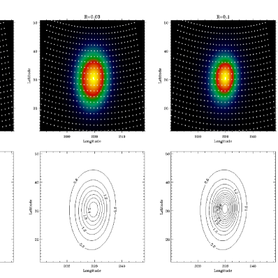
Figure 1: Simulations of an actual Ulysses/GAS particle beam map from 2001 December 12 (in ecliptic coordinates), shown in both image (top) and contour plot (bottom) formats (Wood et al. 2015b). The maps are generated assuming the best-fit He flow vector from Wood et al. (2015a) and a temperature of $T=8500$ K. The color scale in the images is rescaled in each panel so that the maximum is always bright yellow. Maps are computed assuming three different degrees of contamination from O and Ne, corresponding to $R=0.003$ (left), $R=0.03$ (middle), and $R=0.1$ (right).

Figure 2: Single map fits have been performed on synthetic Ulysses particle beam maps, computed assuming various values of R (measuring contamination of O and Ne flux), with map sampling based on 20 real observations (Wood et al. 2015b). For each of the 20 cases, the measured temperature is plotted versus R, with different symbols and line styles indicating different ranges of orbital phase, $\phi$.

The question is then whether $R\approx 0.03$ is low enough to be a plausible value. This is about an order of magnitude higher than the $R=0.0025$ value estimated above based on our best estimates of the quantities in equation (1). Thus, we conclude that heavy element contamination of Ulysses data is unlikely to be the primary cause of the ISM temperature discrepancy between Ulysses and IBEX (Wood et al. 2015b).

3 The Effects of Velocity Distribution Asymmetries on IBEX Data

The IBEX spacecraft is designed to produce a sky map of energetic neutral atom fluxes once every 6 months. In its highly elliptical orbit around Earth, the spinning spacecraft allows its detectors to scan a roughly $14^{\circ}$ wide swath of sky in a given orbit. The spin axis is kept pointed roughly towards the Sun, meaning data from each individual IBEX orbit provides a plot of count rate versus ecliptic latitude. After 7-8 days the orbit is changed so that the new scan plane is rotated typically $7^{\circ}-8^{\circ}$ in longitude. In this way, IBEX gradually covers the entire sky every 6 months.

Figure 3: The first two years of IBEX observations of ISM neutral He. Each panel is a plot of count rate versus ecliptic latitude for a given orbit, with each orbit representing a different longitudinal plane. Green lines are a fit to the data assuming that the source distribution is a simple Maxwellian far from the Sun, while red lines are a fit assuming the distribution far from the Sun is the sum of two Maxwellians, with a separation between the two Maxwellians of $\Delta V=0.4$ km s^-1. Residuals are shown below each panel for both fits.

The interstellar neutrals are only observable at one time each year, with peak fluxes from early January to late February (Möbius et al. 2012). Figure 3 shows the first two years of IBEX observations of the He beam. These are the same data analyzed by Möbius et al. (2012) and Bzowski et al. (2012) in the first assessments of the He flow vector from IBEX. We have fitted these data with an analysis approach essentially identical to that used to analyze Ulysses data (Wood et al. 2015a). Our best fit is shown in Figure 3.

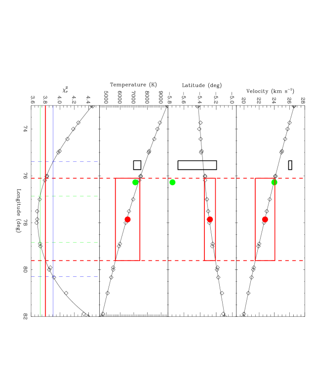
Figure 4: The diamonds show the results of various fits to the first two years of IBEX observations of the ISM He flow, assuming a simple Maxwellian distribution far from the Sun, with one of the four fit parameters held constant in each fit. The upper three panels plot ISM velocity, flow latitude, and temperature versus flow longitude, and the bottom panel plots $\chi^{2}$ versus flow longitude. Horizontal lines in the bottom panel indicate 1, 3, and 5 $\sigma$ confidence levels. The 3$\sigma$ level is used to define the IBEX error boxes in red in the upper 3 panels, which can be compared with the Ulysses error boxes in black, from Wood et al. (2015a). Red circles indicate the best single-Maxwellian IBEX fit, while the green circles indicate the best fit assuming the He flow far from the Sun is the sum of two closely-spaced Maxwellians.

The four free parameters of the fit are flow velocity ($V_{ISM}$), temperature ($T$), flow longitude ($\lambda$), and flow latitude ($\beta$). As shown in Figure 4, the four fit parameters are highly correlated, so you have long tubes in four-dimensional chi-squared space where the fits are reasonably good (Bzowski et al. 2012; Möbius et al. 2012; McComas et al. 2012). Nevertheless, the bottom panel of Figure 4 shows that there is a well-defined $\chi^{2}$ minimum, allowing clear best-fit values and error bars to be computed. Following the example of Wood et al. (2015a) in the analysis of Ulysses data, we use 3$\sigma$ confidence intervals to define the error bounds, leading to the red error boxes in the figure, corresponding to the following values: $V_{ISM}=22.8\pm 1.3$ km s^-1, $\lambda=77.9\pm 1.8^{\circ}$, $\beta=-5.3\pm 0.1^{\circ}$ deg, and $T=6550\pm 890$ K.

These values are basically in agreement with the best-fit values reported by Bzowski et al. (2012), who analyzed these data with a similar forward modeling approach. They can also be compared with our Ulysses measurements ($V_{ISM}=26.08\pm 0.21$ km s^-1, $\lambda=75.54\pm 0.19^{\circ}$, $\beta=-5.44\pm 0.24^{\circ}$, and $T=7260\pm 270$ K), which are shown as black boxes in Figure 4. The apparent inconsistency between the Ulysses and IBEX measurements was initially an issue of much debate, though consideration of more recent observations from IBEX seems to have yielded IBEX measurements more consistent with those of Ulysses (McComas et al. 2015; Leonard et al. 2015; Möbius et al. 2015), with the possible exception of temperature, as discussed in Section 2. The cause of the discrepancy with the first two years of IBEX data seen in Figure 4 has not been explained. However, we note here that if we used 5$\sigma$ error boxes instead of 3$\sigma$, the Ulysses and IBEX boxes would overlap, except for $V_{ISM}$. In any case, our analysis combined with that of Wood et al. (2015a) suggests the Ulysses analysis provides more precise measurements of the flow vector than the IBEX analysis, as indicated by the smaller size of the Ulysses boxes relative to IBEX. The reason for this lies in the ability of Ulysses to observe the He beam from different locations, above and below the ecliptic. This breaks the parameter degeneracies that bedevil IBEX, which can only observe the He beam from one location (Wood et al. 2015a).

The analysis of IBEX data just presented relies on the usual assumption that the ISM He distribution far from the Sun is a simple Maxwellian. The best fit in Figure 3 has $\chi^{2}=3.7$, well above the ideal value of $\chi^{2}\approx 1$, indicating that there is significant room for improvement with regards to how well we are fitting the IBEX data. Perhaps inaccuracies in the single Maxwellian assumption may be at least partly responsible for this. A non-Maxwellian distribution could also potentially affect the best-fit He flow parameters that we have derived. Solar wind distributions are often found to have significant asymmetries (Marsch et al. 1982), so perhaps ISM distributions might as well.

In order to explore the effects of a non-Maxwellian distribution on the IBEX analysis, we experiment with a distribution that is the sum of two closely spaced identical Maxwellians, oriented along the ISM magnetic field line. This is meant to approximate a bi-Maxwellian distribution with $T_{\parallel}>T_{\perp}$. We assume the ISM field is oriented as suggested by the IBEX ribbon, towards ($\lambda$,$\beta$)=($221^{\circ}$,$39^{\circ}$) (Funsten et al. 2009). Fits are then performed to the IBEX data assuming different velocity separations for the two Maxwellians. Figure 5 shows how $\chi^{2}$ varies with assumed separation. The $\chi^{2}$ drops from 3.7 to 2.7 when the separation is increased from $\Delta V=0$ to $\Delta V=0.4$ km s^-1, a surprisingly large amount considering just how small an asymmetry this shift induces in the overall distribution. For comparison, the thermal width of the He distribution for an 8000 K He gas is 5.7 km s^-1. However, Figure 5 also shows that $\chi^{2}$ starts increasing for even larger separations (i.e., larger asymmetries).

Figure 5: The $\chi^{2}$ statistic is plotted versus Maxwellian velocity separation, for fits to the first two years of IBEX data assuming the He flow far from the Sun can be represented as the sum of two closely-spaced Maxwellians.

Figure 3 shows the fit to the data for the $\Delta V=0.4$ km s^-1 fit, and Figure 4 shows the new best-fit He flow parameters that result from the $\Delta V=0.4$ km s^-1 assumption ($V_{ISM}=24.0$ km s^-1, $\lambda=76.3^{\circ}$, $\beta=-5.7^{\circ}$, and $T=7120$ K). We find a lack of robustness for fits assuming these two-Maxwellian distributions, meaning such fits do not have as clean and smooth a $\chi^{2}$ curve as seen in the bottom panel of Figure 4 for the simple Maxwellian fit. The cause of this is uncertain, but as a consequence we do not try to quote error bars for the two-Maxwellian fits at this time. Nevertheless, it is interesting to note from Figure 4 that the best-fit parameters have changed significantly for the $\Delta V=0.4$ km s^-1 fit, and they have actually moved conveniently in the direction of the Ulysses values.

We conclude from this excercise that small asymmetries in the ISM velocity distribution can potentially affect both the quality of fit and the best-fit parameters in analyses of IBEX data. It is therefore worthwhile to explore further the possible effects of non-Maxwellian distributions, which may influence the consistency of parameters derived by IBEX and Ulysses. Future work should involve actual bi-Maxwellian distributions rather than the two-Maxwellian summation approximation.

This work has been supported by NASA award NNH13AV19I to the Naval Research Laboratory.

References

Banaszkiewicz, M., Witte, M., & Rosenbauer, H. 1996, A&AS, 120, 587

Bzowski, M., et al. 2012, ApJS, 198, 12

Bzowski, M., Sokół, J. M., Kubiak, M. A., & Kucharek, H. 2013, A&A, 557, A50

Bzowski, M., Kubiak, M. A., Hłond, M., Sokół, J. M., Banaszkiewicz, M., & Witte, M. 2014, A&A, 569, A8

Funsten, H. O., et al. 2009, Science, 326, 964

Leonard, T. W., et al. 2015, ApJ, 804, 42

Marsch, E., Mühlhäuser, K. -H., Schwenn, R., Rosenbauer, H., Pilipp, W., & Neubauer, F. M. 1982, J. Geophys. Res., 87, 52

McComas, D. J., et al. 2012, Science, 336, 1291

McComas, D. J., et al. 2015, ApJ, 801, 28

Möbius, E., et al. 2012, ApJS, 198, 11

Möbius, E., et al. 2015, ApJS, submitted

Schwadron, N., et al. 2015, ApJS, submitted

Slavin, J. D., & Frisch, P. C. 2008, A&A, 491, 53

Witte, M. 2004, A&A, 426, 835

Wood, B. E., Müller, H. -R., Bzowski, M., Sokół, J. M., Möbius, E., Witte, M., & McComas, D. J. 2015b, ApJS, in press

Wood, B. E., Müller, H. -R., & Witte, M. 2015a, ApJ, 801, 62

Yamamura, Y., & Tawara, H. 1996, Atomic Data and Nuclear Data Tables, 62, 149