Cosmic variance in the nanohertz gravitational wave background

Abstract

We use large N-body simulations and empirical scaling relations between dark matter halos, galaxies, and supermassive black holes to estimate the formation rates of supermassive black hole binaries and the resulting low-frequency stochastic gravitational wave background (gwb). We find this gwb to be relatively insensitive ($\lesssim 10\%$) to cosmological parameters, with only slight variation between wmap5 and Planck cosmologies. We find that uncertainty in the astrophysical scaling relations changes the amplitude of the gwb by a factor of $\sim 2$. Current observational limits are already constraining this predicted range of models. We investigate the Poisson variance in the amplitude of the gwb for randomly-generated populations of supermassive black holes, finding a scatter of order unity per frequency bin below $10$ nHz, and increasing to a factor of $\sim 10$ near $100$ nHz. This variance is a result of the rarity of the most massive binaries, which dominate the signal, and acts as a fundamental uncertainty on the amplitude of the underlying power law spectrum. This Poisson uncertainty dominates at $\gtrsim 20$ nHz, while at lower frequencies the dominant uncertainty is related to our poor understanding of the astrophysical scaling relations, although very low frequencies may be dominated by uncertainties related to the final parsec problem and the processes which drive binaries to the gravitational wave dominated regime. Cosmological effects are negligible at all frequencies.

* Email: ]roebbere@physics.mcgill.ca

1. Introduction

Supermassive black holes, with masses $\gtrsim 10^{6}M_{\odot}$, appear to reside at the center of nearly every moderate to massive galaxy (Kormendy & Richstone, 1995). Mergers between galaxies are relatively common (Lotz et al., 2011), suggesting that the formation of binary supermassive black holes (smbbhs) should also occur regularly (Begelman et al., 1980). Such smbbhs should produce considerable gravitational radiation in a frequency band of $\sim 10^{-9}$–$10^{-7}$ Hz (e.g. Thorne, 1987; Maggiore, 2008). Careful monitoring of arrival times of radio pulses from a large number of individual pulsars could allow detection of this gravitational radiation. This idea is implemented in pulsar timing arrays (ptas) (Hellings & Downs, 1983; Foster & Backer, 1990; Shannon et al., 2015; Arzoumanian et al., 2015; Lentati et al., 2015). Recent estimates (e.g. Sesana, 2013b; McWilliams et al., 2014; Ravi et al., 2015; Rosado et al., 2015) suggest that detection of gravitational radiation with ptas may occur in the near future.

The gravitational radiation due to smbbhs is expected to form an approximately isotropic stochastic background, with a spectrum at relatively low frequencies set by the well-known rate at which the binary’s orbit decays due to emission of gravitational radiation (Phinney, 2001). The amplitude is set by the total population of emitting smbbhs, which can be estimated from the current understanding of galaxy merger rates and the apparent ubiquity of supermassive black holes in galaxies of at least moderate size.

The amplitude of gravitational radiation produced by smbbhs also depends on a large number of environmentally dependent and often poorly-understood astrophysical variables: the characteristic masses of black holes in the centers of galaxies (Lauer et al., 2007; Kormendy & Ho, 2013); merger rates of the relevant galaxies; dynamical friction (Chandrasekhar, 1943; Boylan-Kolchin et al., 2008); the physical mechanisms removing sufficient energy and angular momentum from the binary system (e.g. Kocsis & Sesana, 2011; Ravi et al., 2014) to bring the black holes close enough to eventually merge through the emission of gravitational radiation (the ‘final parsec problem,’ see Merritt & Milosavljević, 2005); the eccentricity of the binary black hole orbits (Peters & Mathews, 1963); and the evolution of all of these effects as a function of cosmic time.

There have been many predictions of the expected gravitational wave background (hereafter gwb) produced by smbbhs, with a variety of approaches used: semi-analytic predictions with merger rates based on the Press-Schechter formalism (Wyithe & Loeb, 2003; Enoki et al., 2004; Enoki & Nagashima, 2007; Sesana et al., 2004, 2008; Rosado, 2011); N-body simulations dressed with black holes using prescriptions for how various types of galaxies form (Sesana et al., 2009; Kocsis & Sesana, 2011; Kulier et al., 2015; Ravi et al., 2014); and empirically-based estimates of the galaxy merger rate from observed numbers of close pairs (Jaffe & Backer, 2003; Sesana, 2013b; Ravi et al., 2015). In all cases, uncertainties in how black holes populate galaxies lead to a large theoretical uncertainty in the expected gwb level.

In this paper we use very large cosmological N-body simulations (dark matter only) with up-to-date cosmological parameters and recent estimates of various scaling relations to relate dark matter halo mass with black hole mass and calculate the expected gwb. We will briefly explore the uncertainty in these astrophysical scaling relations, but will primarily focus on the fundamental scatter in the gwb due to Poisson statistics in the population of smbbhs.

The organization of the paper is as follows: In Section 2 we describe our procedure for calculating the gwb starting with merger trees from N-body simulations. We explain our prescription for placing galaxies within dark matter halos and black holes within galaxies, as well as our Monte Carlo sampling of the population of smbbhs and subsequent calculation of the gwb. In Section 3 we discuss the characteristics of our predicted signal. This includes the amplitude of the signal, differences between simulations, exploration of the effects of astrophysical uncertainties, as well as the scatter in the amplitude as a function of frequency for many different Monte Carlo realizations. Section 4 presents our conclusions and discussion of future directions.

2. Calculating the Gravitational Wave Background

In this section, we explain how we generate a representative population of smbbhs beginning with dark matter merger trees from N-body simulations, and calculate the gwb produced by this population in the pta frequency band. In the subsections below we discuss the dark matter simulations used, describe how we populate dark matter halos with black holes, explain our prescription for calculating binary black hole formation rates from halo merger trees, review the calculation of gravitational wave strain from smbbhs, and finally put all these pieces together to describe how we produce individual realizations of the population of smbbhs and calculate the resulting gwb.

2.1. N-body Simulations

	Dark Sky	MultiDark
$\Omega_{m}$	0.32	0.27
$\Omega_{\Lambda}$	0.68	0.73
$h$	0.67	0.7
$\sigma_{8}$	0.83	0.82
Box volume $(\text{Mpc}^{3}/h^{3})$	$1000^{3}$	$1000^{3}$
Particle mass ($M_{\odot}/h$)	$10^{10}$	$9\times 10^{9}$
Number of particles	$2048^{3}$	$2048^{3}$
Number of snapshots	13	43
Longest timestep (Myr)	1600	500
Shortest timestep (Myr)	470	110
Lowest snapshot redshift	0	0
Highest snapshot redshift	4	10

Table 1Properties of the simulations and their merger trees

We begin our calculation with merger trees from two recent large-scale dark matter simulations. Their properties are summarized in Table 1. The first is the Dark Sky simulation (Warren, 2013), which uses a set of cosmological parameters based on Planck (Planck Collaboration XVI, 2014). The second is MultiDark, or Big Bolshoi (Riebe et al., 2011; Prada et al., 2012), which uses the same initial conditions as the Bolshoi simulation (Klypin et al., 2011), and is consistent with wmap5 parameters (Komatsu et al., 2009), and remains consistent with wmap9 (Hinshaw et al., 2013). The wmap5 and Planck cosmologies are similar, particularly for the value of $\sigma_{8}$, which is important for structure formation. Differences remain, especially for the parameters $\Omega_{m}$ and $h$. Both of these cosmologies are significantly different from that chosen for the Millennium simulation, which is consistent with the wmap1 cosmology (Springel et al., 2005).

We use merger trees produced from these simulations by the halo finder Rockstar (Behroozi et al., 2013c) and merger tree code Consistent Trees (Behroozi et al., 2013b). Throughout this work, we will use the term “halo” to mean any subhalo or host halo listed in the merger trees.

Halo mass functions for Dark Sky and MultiDark at $z=0$ and $z=1$ are shown in the top left panel of Figure 1. The two simulations have similar volumes and mass resolutions. Both mass functions are essentially complete between $\sim 10^{12}M_{\odot}$ and $\sim 10^{15}M_{\odot}$ at low redshift. The slight offset in the amplitudes of the halo mass functions is a result of their different cosmologies. In addition to the cosmology, the two simulations differ in their time resolution and the redshift range in which the snapshots are taken. We will consider the effects of these differences throughout our calculation.

2.2. Populating Halos with Black Holes

Supermassive black holes are correlated with properties of their host galaxies (for a review, see Kormendy & Ho, 2013). In order to make predictions about the population of supermassive black holes, we first need to characterize the population of galaxies inhabiting the dark matter halos in each simulation. We use the scaling relation between halo mass and galaxy stellar mass calculated by Behroozi et al. (2013a) to derive the stellar masses of galaxies inside the halos.

This relation was derived by requiring consistency between abundance matching calibrated to observed galaxy stellar mass functions and calculations of the star formation rate. They fit the stellar mass–halo mass relation to a 5-parameter model which behaves as a power law at low mass and a subpower law at high mass and varies as a function of redshift between $0<z<8$. This form was chosen to provide a better fit to the observed stellar mass function than the commonly-used double power law (Behroozi et al., 2013a). Their relation also contains an evolving intrinsic scatter in the stellar mass at low redshifts.

We use this relation to populate halos in our two simulations with galaxies. The intrinsic scatter is accounted for by randomly drawing from a normal distribution with the appropriate standard deviation. The resulting stellar mass functions are shown in the bottom left panel of Figure 1. The evolution of the stellar mass function at masses above $10^{11}M_{\odot}$ is not significant at redshifts $0<z<1$, which will turn out to be the redshift range of most interest for our results. Below $10^{11}M_{\odot}$, the stellar mass function begins to drop due to the minimum halo mass resolved in the simulations. A small offset between the two simulations remains, but is less significant than in the halo mass functions.

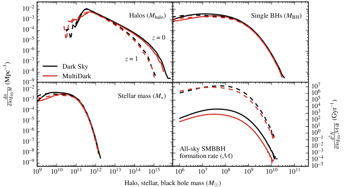
Figure 1.— Halo, stellar, black hole, and smbbh mass functions calculated for the Dark Sky and MultiDark merger trees as described in the text. Solid lines show the mass functions at $z=0$ and dashed lines represent $z=1$, except for binaries, for which solid lines represent an interval of $0\lesssim z\lesssim 0.05$ and dashed lines represent $1\lesssim z\lesssim 1.5$. The resolution limit can be clearly seen in the peaks of the halo mass functions between $10^{11}M_{\odot}$ and $10^{12}M_{\odot}$. This limit is then propagated with scatter to the galaxy, single black hole, and smbbh mass functions. The smbbh formation rates represent the number of binaries produced per Gyr, integrated over the volume in each redshift bin. The shift in amplitude between the two redshift intervals is primarily due to the much greater volume at $1<z<1.5$ than at $0<z<0.05$.

We model different populations of galaxies by splitting galaxies between ‘quiescent’ and ‘star-forming’ populations based on the evolving mass functions from Moustakas et al. (2013). After this split, we calculate bulge masses for each population based on the relations shown in Figure 1 of Lang et al. (2014). Our model does not take into account environmental dependence or merger history, but is calculated for the population as a whole.

With this calculation of the galaxy bulge mass, we can determine the distribution of black holes. We place black holes inside the galaxies using the Kormendy & Ho (2013) stellar bulge mass–black hole mass scaling relation, randomly drawing the black hole masses according to the intrinsic scatter:

$$\left(\frac{M_{\text{BH}}}{10^{9}M_{\odot}}\right)=0.049\left(\frac{M_{\star}}{10^{11}M_{\odot}}\right)^{1.16}\mkern-5.0mu plus -5.0mu\mkern-5.0mu plus -5.0mu,\quad\text{scatter}=0.29\text{ dex}.$$ (1)

This relation incorporates recent measurements and recalculations of black hole masses, especially for the largest black holes present in brightest cluster galaxies, which may have been systematically underestimated previously (e.g. Gebhardt et al., 2011; Hlavacek-Larrondo et al., 2012; McConnell et al., 2012; Rusli et al., 2013). Additionally, they restrict the sample of black holes to those with host galaxies that are ellipticals and spirals with so-called classical bulges in order to form a clean sample of “objects that are sufficiently similar in formation and structure” (Kormendy & Ho, 2013).

We do not apply any explicit prescriptions for black hole mass growth through accretion (or mergers). Instead, we assume that this scaling relation applies at all redshifts, implicitly requiring that black holes grow along with their host galaxies. For merging halos, the scaling relations are applied at the timestep before merger. The resulting black hole mass functions are shown in the top right panel of Figure 1. The mass functions are remarkably consistent for $M_{\text{BH}}\gtrsim 10^{9}M_{\odot}$ for $0<z<1$. For $M_{\text{BH}}\lesssim 10^{8}M_{\odot}$, the differences between simulations are once more due to the mass resolution of the simulations. The point at which the two simulations deviate shows where the mass functions become untrustworthy. This mass changes somewhat with redshift, but remains of order $10^{8}M_{\odot}$.

In addition to the uncertainty in our mass functions due to the simulation resolution, we expect additional error due to our choice of scaling relations. In particular, the relationship between stellar mass and bulge mass, which is related to galaxy morphology, is not well known. Moreover, the distribution of ellipticals versus spirals depends strongly on environment through the well-studied morphology–density relation (Dressler, 1980). Accurate modeling of the merger rate for each galactic morphological type would require detailed semi-analytic models, so we treat the relation between total stellar mass and bulge mass as an astrophysical uncertainty in our calculations.

The uncertainty in the $M_{\text{bulge}}$–$M_{\text{BH}}$ relations increases at both high and low black hole mass. For the latter case, there is a significant population of black holes which no longer be fit tight scaling relations (Kormendy & Ho, 2013). As a result, our scaling relations are inaccurate for $M_{\text{BH}}\lesssim 10^{8}M_{\odot}$ and for $M_{\text{BH}}\gtrsim 10^{10}M_{\odot},$ but the effect of this on the signal is likely to be smaller than that due to the mass resolution.

2.3. Black Hole Binaries Form When Halos Merge

We use the supermassive black hole mass functions calculated in the previous section to assign smbbhs to merging halos identified by the merger trees. Consistent Trees (Behroozi et al., 2013b) builds merger trees by tracking halos across multiple timesteps. It uses this history to determine when a halo (typically a subhalo) has merged into a larger halo (the halo creating the strongest tidal field). We use the halo masses calculated at the timestep before merger to calculate black hole masses.

For each halo merger we calculate the masses of the black holes residing in the two largest dark matter halo progenitors, and assign an equivalent binary to the descendant halo. We remove minor mergers from our list by performing a cut in the stellar mass ratio of progenitors such that $M_{\star,2}/M_{\star,1}\geq 0.05$, where $M_{\star,1}$ is the progenitor with the larger stellar mass and $M_{\star,2}$ is the progenitor with the smaller stellar mass. We assume that dynamical friction proceeds quickly (see Dotti et al., 2007) and that the final parsec problem is solved in all cases, so that all black holes form a binary as soon as the progenitor halos merge. We do not consider any accretion onto either black hole during the galaxy merger or the possibility of triple systems.

With these assumptions, we can calculate the mass function of smbbhs formed between snapshots for each simulation. We parameterize the mass of black hole binaries using the chirp mass:

$$\mathcal{M}\equiv\mu^{3/5}M_{\text{tot}}^{2/5}=\frac{(m_{1}m_{2})^{3/5}}{(m_{1}+m_{2})^{1/5}}$$ (2)

and the black hole mass ratio

$$q=\frac{m_{2}}{m_{1}},\quad m_{1}>m_{2},$$ (3)

where $m_{1}$ and $m_{2}$ are the masses of the black holes in the binary. We allow a mass range of $10^{6}M_{\odot}<\mathcal{M}<10^{10.5}M_{\odot}$ and a black hole mass ratio range of $5\times 10^{-4}<q<1$ to ensure that all binaries producing significant signal are included. The mass function is logarithmically binned in both $\mathcal{M}$ and $q$, with bin sizes chosen so that bins are always less than $10\%$ of each quantity.

In order to ensure a smooth distribution which accounts for the intrinsic scatter in the scaling relations, we repopulate the merging halos in each simulation 10,000 times and use the average to calculate the final mass function of smbbhs. Although we are able to account for the scatter in the scaling relations this way, we only have a single set of merger trees for each simulation, and so cannot similarly calculate the scatter in the merger rates of halos. We do not expect this to significantly affect our results, since most halos hosting black holes of interest are well-represented in the simulation boxes.

The rate at which smbbhs of different masses are produced is shown in the bottom right panel of Figure 1. Rates are derived by counting the number of mergers per chirp mass bin, integrating over volume, and dividing by the time elapsed for each redshift range. We show the intervals $0\lesssim z\lesssim 0.05$ and $1\lesssim z\lesssim 1.5$, which correspond to single timesteps for Dark Sky and the sum of multiple timesteps for MultiDark. Dark Sky has a slightly higher binary black hole production rate than MultiDark at low redshift, which largely disappears by $z\sim 1$. This is due to a higher halo merger rate at low redshifts.

2.4. Gravitational Radiation from Black Hole Binaries

At separations $\ll 1$ pc, the evolution of smbbhs becomes dominated by emission of gravitational radiation. As it emits gravitational waves, the radius of a binary will shrink and the orbit will circularize. For a binary in a circular orbit, the gravitational radiation emitted will be at a single frequency $f_{\text{emit}}=2f_{\text{orbit}}$. If the binary is at cosmological distances, the frequency seen by an observer will be redshifted such that

$$f_{\text{obs}}=\frac{f_{\text{emit}}}{1+z}=\frac{2f_{\text{orbit}}}{1+z}.$$ (4)

As it emits, the binary’s orbit will decay and the frequency will increase as (e.g. Thorne, 1987; Cutler & Flanagan, 1994; Wyithe & Loeb, 2003; Sesana et al., 2008)

$$\frac{df_{\text{emit}}}{dt}=\frac{96}{5}\frac{(G\mathcal{M})^{5/3}}{\pi c^{5}}(\pi f_{\text{emit}})^{11/3},$$ (5)

or equivalently, the relationship between the emitted frequency at a time $t$ after the binary begins emitting at frequency $f_{0}$ can be written as

$$(\pi f_{0})^{-8/3}-(\pi f_{\text{emit}})^{-8/3}=\frac{256}{5}\frac{(G\mathcal{M})^{5/3}}{c^{5}}\,t.$$ (6)

We consider binaries in circular orbits emitting gravitational waves at frequencies between the initial frequency where gravitational radiation becomes the dominant mechanism bringing the black holes together, and a final frequency just before coalescence.

We choose our initial frequency based on the Quinlan (1996) estimate for when gravitational radiation becomes efficient:

$$f_{\text{0}}=2.2\text{ nHz}\left(\frac{m_{1}+m_{2}}{2\times 10^{8}M_{\odot}}\right)^{1/5}\left(\frac{(10^{8}M_{\odot})^{2}}{m_{1}m_{2}}\right)^{3/10}\mkern-5.0mu plus -5.0mu.$$ (7)

Although the exact frequency where gravitational radiation dominates over other processes bringing the binary together depends on how the final parsec problem is solved, changing our initial frequency does not significantly affect our results, provided it is neither well inside the visible frequency range, nor sufficiently low that most binaries will not merge within a Hubble time. Both of these situations could be reproduced by astrophysical processes related to the final parsec problem. The first might be caused by high eccentricities or environmental effects which dominate even when the binaries emit significant gravitational radiation (e.g. Enoki & Nagashima, 2007; Kocsis & Sesana, 2011; Ravi et al., 2014). The second would occur if the final parsec problem is not solved for all binaries (e.g. McWilliams et al., 2014).

Following Hughes (2002), we estimate the final frequency from the innermost stable circular orbit for a Schwarzschild black hole of equivalent mass:

$$f_{\text{{isco}}}=22\,\mu\text{Hz}\left(\frac{2\times 10^{8}M_{\odot}}{m_{1}+m_{2}}\right).$$ (8)

Since the orbit of the binary decays extremely rapidly towards the end of its lifetime, the exact value chosen for this frequency does not significantly affect the total lifetime of the binary nor the range of frequencies over which it is observed.

Using Equation (missing) 6 and the above initial and final frequencies, we can write the emitted frequency as a function of time more simply:

$$f_{\text{emit}}(t)=\frac{1}{\pi}\left[\left(1-\frac{t}{T}\right)(\pi f_{0})^{-8/3}+\frac{t}{T}\left(\pi f_{\text{{isco}}}\right)^{-8/3}\right]^{-3/8}$$ (9)

where $T$ is the lifetime of the binary, namely the time that passes between when the binary begins emitting at $f_{0}$ and when it reaches $f_{\text{{isco}}}$. We will use this relation in the next section to randomly sample the frequency distribution of gravitational wave sources.

The amplitude of gravitational waves produced by a single binary at this characteristic frequency, averaged over angle and polarization, is given by (e.g. Thorne, 1987):

$$h(f_{\text{emit}})=\sqrt{\frac{32}{5}}\frac{(G\mathcal{M})^{5/3}}{c^{4}R(z)}(\pi f_{\text{emit}})^{2/3},$$ (10)

where $R(z)$ is the comoving distance to the smbbh.

2.5. The GWB Produced by a Population of Binaries

The gwb is the result of an incoherent sum of many gravitational wave signals and depends on the properties of the population which produces it. We wish to investigate the gwb from a statistical point of view, so we will use Monte Carlo selection to generate many different realizations of the population of binaries observed to be emitting gravitational radiation.

In particular, for each redshift interval $\Delta z_{i}$, we will convert the comoving number density of binaries produced within the simulation box, $n(\mathcal{M},q,\Delta z_{i})$, into the distribution $N^{\text{obs}}_{i}(\mathcal{M},q)$ representing the population of smbbhs seen by an observer in a universe with the same underlying distributions as the simulation. We will draw from this distribution to simulate the population of smbbhs out to $z\sim 4$ in an individual realization of the universe. This process is analogous to that done by e.g. Sesana et al. (2008).

To begin, we calculate the comoving number density of binaries with $\mathcal{M}\geq 10^{6}M_{\odot}$ formed between each snapshot in the simulation, as described in Section 2.3. We write the comoving number density as $n(\mathcal{M},q,\Delta z_{i})$. We then convert this to the expected number of binaries formed within the volume of the shell corresponding to the redshift interval $\Delta z_{i}$:

$$N_{i}(\mathcal{M},q)=n(\mathcal{M},q,\Delta z_{i})V_{c}(\Delta z_{i}).$$ (11)

Next, we account for the fact that binaries of different masses have different lifespans, and therefore are not equally likely to be observed. As a result of the mass dependence in Equation (missing) 5, heavier binaries merge much more quickly than light ones, and so any observation of the smbbh population will tend to see a smaller percentage of heavy binaries than would naively be expected from the bottom right panel of Figure 1.

We use this property to transform the distribution of binaries formed within a redshift shell to the distribution of binaries seen to be emitting gravitational radiation by an observer at $z=0$:

$$N^{\text{obs}}_{i}(\mathcal{M},q)=N_{i}(\mathcal{M},q)\times\text{min}\left(\frac{T(\mathcal{M},q)}{\Delta t_{i}},1\right),$$ (12)

where $T(\mathcal{M},q)$ is the lifetime of binaries in the bin and $\Delta t_{i}$ is the time between snapshots. This distribution represents the number of sources present on our lightcone. We will draw from this population of smbbhs to produce the gwb.

For each redshift interval $z_{i}$, we Poisson sample the distribution $N^{\text{obs}}_{i}(\mathcal{M},q)$ to produce a single realization of the population. This is necessary since many bins of $N^{\text{obs}}_{i}(\mathcal{M},q)$ have less than one source on average, particularly at low redshifts and high masses where the resulting gravitational signal is brightest.

Having drawn the masses of the binaries in our population, we select corresponding redshifts and frequencies at which the binaries emit. Since all binaries are already on our lightcone, we choose frequencies by drawing randomly from within each binary’s lifetime, and then converting that time to a frequency according to Equation (missing) 9. We choose redshifts by drawing from a volume-weighted distance distribution corresponding to the redshift interval, and then converting the distance to a redshift. This is important at low redshifts in order to avoid spurious sources at redshifts very close to zero. We calculate the properties of the population of binaries anew for each timestep, neglecting any binaries which might still exist in the next, since most timesteps are longer than the lifetimes of the binaries producing most of the signal.

With this population of observed binaries we can calculate the total strain in the gwb for a single realization of the universe. To allow comparison with pta upper limits, we bin the signal by the inverse of the total observation time. The minimum frequency is likewise set by the total observation time and the maximum frequency is set by the cadence. To illustrate, we will assume a pta observation time of 25 years with observations occurring every six weeks. The frequency bins therefore have widths

$$\Delta f=\frac{1}{T_{\text{obs}}}=(\text{25 years})^{-1}\approx 1.3\text{ nHz},$$ (13)

and are located between $f_{\text{min}}\approx 1.3$ nHz and

$$f_{\text{max}}=\frac{1}{2}(\text{6 weeks})^{-1}\approx 100\text{ nHz}.$$ (14)

We will test the effect of these assumptions in Section 3.4.

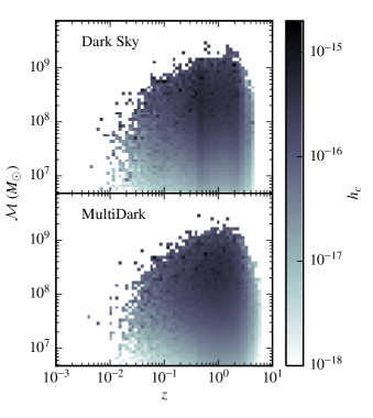
Figure 2.— A single Monte Carlo realization for each simulation of the total strain produced by a population of smbbhs as a function of chirp mass and redshift. We include all binaries with frequencies between $f_{\text{min}}$ and $f_{\text{max}}$. Varying strain amplitude between adjacent bins is mostly due to sources emitting gravitational waves at different frequencies.

We calculate the gravitational radiation produced by each binary according to Equation (missing) 10. The characteristic strain $h_{c}$ in each bin $f_{n}$ is given by a weighted sum over the squared strain of all sources observed at frequencies $f_{n}<f_{i}^{\text{obs}}<f_{n}+\Delta f$ (Thorne, 1987):

$$h_{c}(f_{n})=\left(\sum_{i}h_{i}^{2}\!\left(f_{i}^{\text{emit}}\right)f_{i}^{\text{obs}}t_{i}^{\text{bin}}\right)^{1/2},$$ (15)

where $t_{i}^{\text{bin}}\leq T_{\text{obs}}$ is the total time that the binary is observed at a frequency within bin $f_{n}$. The vast majority of sources will remain in the same frequency bin for the entire observation. For these binaries, $t_{i}^{\text{bin}}=T_{\text{obs}}$, and the extra factor in Equation (missing) 15 becomes the standard $f_{i}^{\text{obs}}/\Delta f$.

However, for the frequency range and binning that we consider, we cannot neglect evolving binaries despite their rarity. For a binary to be shrinking quickly enough to change frequency bins over the course of the observation time, it must typically have a high mass and be very tight. From Equation (missing) 10 it is clear that such binaries can produce particularly strong signals. We therefore calculate the redshifted frequency for each source at a time $t+T_{\text{obs}}$. For those binaries which have changed in frequency by at least one bin, we calculate the time spent in each bin, and divide up the signal accordingly.

A single realization of the gwb for each simulation as a function of $\mathcal{M}$ and $z$ is shown in Figure 2. Although most binaries are at moderate mass and high redshift, most of the strain comes from binaries with $\mathcal{M}\gtrsim 10^{8}M_{\odot}$ and $0.1\lesssim z\lesssim 2$. Both simulations become incomplete for masses below $10^{8}M_{\odot}$, but the strain produced by low mass binaries primarily decreases due to the scaling of $h\sim\mathcal{M}^{5/3}$, as can be seen at low redshifts where the bins are populated by individual binaries. On the other end of the scale, black holes with $\mathcal{M}\sim 10^{10}M_{\odot}$ only rarely appear in individual realizations. Neither the increased inaccuracy of the scaling relations at low or very high black hole mass nor the missing low-mass binaries due to the simulation resolution should significantly affect the total strain.

3. Discussion

In this section we present our calculated amplitude of the gwb and compare with other recent predictions. We discuss two forms of uncertainty on the amplitude of the gwb: that due to uncertainty in the astrophysical scaling relations and the variance of the gwb spectrum between individual realizations of the smbbh population. Finally, we discuss the dependence of the realization-to-realization variance on the choice of frequency bins.

3.1. Amplitude of the Characteristic Strain Spectrum

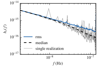
Figure 3.— Three separate realizations of the gwb for MultiDark along with the median and rms gwb calculated for the entire sample of 5,000 realizations. At high frequencies, the median signal drops below the canonical power law, and the amplitudes in adjacent bins become increasingly uncorrelated for non-evolving sources.

The form of the gwb strain spectrum was calculated analytically by Phinney (2001), who determined that any sufficiently large isotropic population of compact objects in circular orbits decaying due to the emission of gravitational radiation should produce a stochastic background with a $2/3$ power law frequency spectrum. In the real universe, the finite population of black holes will prevent the gwb from attaining power-law behavior, but a power law is expected to be approximately accurate for a subset of frequencies and represents the expected spectrum for an unobservable ensemble of realizations of the gwb (Sesana et al., 2008). Pulsar timing arrays often search for a power law stochastic signal, and report constraints on the amplitude $A$ given by

$$h_{c}(f)=A\left(\frac{f}{1\text{ yr}^{-1}}\right)^{-2/3}.$$ (16)

To date, the strongest upper bound on a power law frequency spectrum come from Shannon et al. (2015) who rule out a power law gwb with amplitude $A>1\times 10^{-15}$ at 95% confidence. Other ptas (Arzoumanian et al., 2015; Lentati et al., 2015) report similar constraints.

We generate 5,000 separate realizations of the gwb for each simulation, as described in Section 2.4. Using the ensemble of spectra for each simulation, we calculate the rms and median strain. An example is shown in Figure 3, where we plot three individual realizations of the spectrum, along with the rms and median strain. As in Sesana et al. (2008), at frequencies $\lesssim 10$ nHz the gravitational wave spectra are smooth and very similar to both the rms and median signals. For frequencies $\gtrsim 20$ nHz, the amplitudes in each frequency bin vary widely and the median strain drops noticeably below the rms strain.

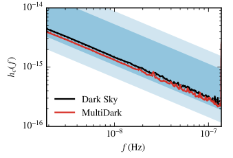
Figure 4.— Rms amplitudes (solid lines) for the gwb in both simulations, as calculated for 5,000 realizations assuming a 25 year observation time. The dotted lines represent best-fit $2/3$ power laws for Dark Sky (black) and MultiDark (red). Shaded regions show $95\%$ confidence intervals on other recent predictions of the gwb. The larger pale blue region represents the Sesana (2013b) predictions when using the McConnell & Ma (2013) scaling relations, which are most comparable to our choice. The smaller blue shaded region shows the Ravi et al. (2015) prediction.

The rms spectrum (see Figure 4) is very similar to the expected $2/3$ power law, but with occasional spikes due to the presence of an extremely rare and bright source in that bin for one of the 5,000 realizations. The best fit $2/3$ power laws have amplitudes $A_{D}=6.84\times 10^{-16}$ and $A_{M}=6.14\times 10^{-16}$.

We also calculate the semi-analytic amplitude for each simulation by direct integration (Phinney, 2001):

$$h_{c}^{2}(f)=\frac{4G}{\pi c^{2}f^{2}}\int_{0}^{\infty}\text{d}z\int_{0}^{\infty}\text{d}\mathcal{M}\,\frac{\text{d}^{2}n}{\text{d}z\,\text{d}\mathcal{M}}\frac{1}{1+z}\frac{\text{d}E_{\textsc{gw}}}{\text{d}\ln f_{\text{emit}}},$$ (17)

where $n$ is the comoving number density and

$$\frac{\text{d}E_{\textsc{gw}}}{\text{d}\ln f_{\text{emit}}}=\frac{\pi}{3G}\frac{(G\mathcal{M})^{5/3}}{(\pi f_{\text{emit}})^{1/3}}.$$ (18)

The resulting semi-analytic amplitudes are $A_{\text{D, SA}}=6.89\times 10^{-16}$ and $A_{\text{M, SA}}=6.13\times 10^{-16}$, consistent with their respective Monte Carlo counterparts. The slightly larger difference for Dark Sky is likely due to its coarser redshift resolution.

The difference in amplitude between the simulations is small but consistent with differences due to the initial halo mass functions and halo merger rates at low redshift. Our rms amplitudes are a factor of $\sim 2$ below the latest power law upper limits from nanograv (Arzoumanian et al., 2015), and a factor of $\sim 1.5$ below the recent best upper limits from ppta (Shannon et al., 2015). Our rms amplitudes are consistent with the predictions of Sesana (2013b) and Ravi et al. (2015), despite the different approaches used.

3.2. Astrophysical Uncertainty

In this section, we briefly explore the effect of uncertainty in our astrophysical assumptions. In particular, astrophysical uncertainties affect our calculations within the:

• halo mass–stellar mass scaling relations,

• calculation of the bulge mass as a fraction of the total galaxy stellar mass,

• bulge mass–black hole mass scaling relation,

• galaxy merger rates, and

• processes used to form smbbhs and overcome the final parsec problem.

The effect of the final parsec problem and of the putative astrophysical processes which allow it to be overcome is a question of considerable scope. We will leave its exploration for later work. Additionally, we use the halo merger rates from the simulations to determine galaxy merger rates. Some uncertainty in the merger rate can be associated with the difference in amplitude between simulations, but we do not explore uncertainty in the galaxy merger rate further. In what follows, we focus on the uncertainties due to the other three astrophysical processes listed above. Results are shown in Figure 5.

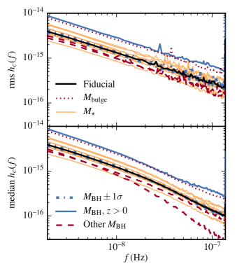
Figure 5.— Rms and median strain of our fiducial MultiDark model (black). Other lines show models with varying astrophysical scaling relations. The single dotted red line represents a model where bulge mass equals stellar mass for all galaxies. The thin yellow lines show 10 randomly selected points in the parameter space of the Behroozi et al. (2013a) stellar mass–halo mass relations. The dash-dotted blue lines very close to the fiducial model are the $\pm 1\sigma$ Kormendy & Ho (2013) $M_{\text{bulge}}$–$M_{\text{BH}}$ relations. The dashed red lines represent the McConnell & Ma (2013) (upper) and Graham (2012) (lower) $M_{\text{bulge}}$–$M_{\text{BH}}$ relation. The solid blue line is the Kormendy & Ho (2013) relation, but incorporating redshift evolution as in Bennert et al. (2010).

Our basic model for the galaxy stellar mass function uses the halo mass functions of the two simulations and the best-fit parameters of the Behroozi et al. (2013a) stellar mass–halo mass scaling relation. To explore the uncertainty in this scaling relation, we repeat the calculation of the gwb, using 10 randomly chosen points from the allowed parameter space in the stellar mass–halo mass relation (P. Behroozi, private communication). The results are shown as the thin yellow lines in Figure 5. Although most of the models have amplitudes very close to that of our basic model, outliers in both directions differ by a factor of $\sim 2$.

As discussed in Section 2.2 our fiducial model calculates the bulge mass of galaxies by first assigning them to ‘quiescent’ or ‘star-forming’ populations and then using a population-dependent relationship between bulge mass and stellar mass. This approach neglects the effects of environment and merger history. To estimate the effect of our assumptions on the amplitude of the gwb, we use an alternate model in which the bulge mass equals the stellar mass for all galaxies, effectively assuming that all galaxies are elliptical. This is not particularly plausible–for nearby galaxies with stellar masses $\gtrsim 10^{11}M_{\odot}$, elliptical and lenticular galaxies appear to make up roughly 40% of the total population (Hoyle et al., 2012; Wilman & Erwin, 2012). Instead, we use this as an upper limit on the amplitude that could be produced by varying this relation. The resulting gwb is shown as a dotted red line in Figure 5, and has an amplitude a factor of 2 above the fiducial model.

To estimate the uncertainty on the gwb amplitude due to the black hole scaling relations, we repeat our calculations using the $\pm 1\sigma$ parameters from the Kormendy & Ho (2013) $M_{\text{bulge}}$–$M_{\text{BH}}$ scaling relations. The resulting spectra are shown as dot-dashed blue lines in Figure 5. They remain close to the original model. The two dashed red lines are calculated using the McConnell & Ma (2013) and the Graham (2012) $M_{\text{bulge}}$–$M_{\text{BH}}$ scaling relations. They are both within a factor of 2 of the amplitude in our fiducial model, although the Graham (2012) broken power law model noticeably changes the shape of the median at high frequencies, and the rms spectrum is slower to converge to the expected shape. This is not surprising given that this scaling relation produces relatively more low-mass binaries; see the discussion in Section 3.3.

We explore the possibility of evolution in the black hole scaling relation with redshift by applying the Bennert et al. (2010) scaling of $M_{\text{BH}}/M_{\text{bulge}}\propto(1+z)^{1.4}.$ This produces an amplitude a factor of $\sim 2$ above our standard model, shown as the solid blue line in Figure 5. However, this model might be better formulated to include a variant bulge mass model, since Bennert et al. (2010) do not see any evolution with total galaxy luminosity, suggesting that bulge evolution plays a significant role in any evolution of the black hole scaling relation.

The primary effect of the different parameter choices for the varying relations is a vertical shift in amplitude in all bins; the shape of the spectrum is not strongly affected unless the black hole mass function changes significantly. The range of amplitudes produced by astrophysical variants overlaps the Ravi et al. (2015) and Sesana (2013b) 95% limits shown in Figure 4. The dominant effects appear in the stellar bulge mass calculation, but this may be modified by black holes growing at different eras from bulges. Uncertainties in the stellar mass scaling relations and black hole scaling relations are smaller but of the same order of magnitude.

The range in amplitudes suggested by our models for the astrophysical uncertainty is significantly constrained by pta measurements. The ppta upper limit on a power law gwb is within a factor of two of our fiducial amplitude, and rules out our variant models with either an evolving $M_{\text{BH}}$–$M_{\text{bulge}}$ relation or an all-elliptical galaxy population. The nanograv upper limit does not directly rule out any model presented here, but is in tension with the highest models.

3.3. Variance from a Finite Number of Sources

In this section we discuss variance in the amplitude and shape of the gwb spectrum resulting from only having a single realization of the population of smbbhs. In contrast to the effect of unknown astrophysics discussed in the previous section, this scatter is innate: it is the result of having only a single observation of the gwb, and is directly analogous to the well-known effect of cosmic variance in the analysis of the cosmic microwave background power spectrum. It has been discussed previously in e.g. Ravi et al. (2012); Cornish & Sesana (2013), with earlier related work by Jaffe & Backer (2003) and Sesana et al. (2008).

The two forms of variance affect the spectrum of the gwb differently. The astrophysical effects discussed in the previous section produce a systematic offset in the amplitude, while maintaining a power law spectrum. In contrast, the variance due to only having a single realization does not produce a systematic offset in amplitude, but rather changes the spectrum away from a power law and adds an uncorrelated component to the amplitudes of the gwb in individual frequency bins.

In Figure 3 we show three realizations of the gwb along with the rms and median strains calculated for the full set of 5,000 realizations. Although the rms strain can be described by a power law, the shape of each realization cannot. Each spectrum contains many spikes and dips due to the presence (or lack thereof) of bright individual sources (cf. Rajagopal & Romani, 1995; Jaffe & Backer, 2003; Sesana et al., 2008; Kocsis & Sesana, 2011). At frequencies $\gtrsim 20$ nHz the rms signal is mostly due to these rare, high-amplitude events. The median amplitude, as was originally found by Sesana et al. (2008), dips below the rms signal. At high frequencies, the scatter in the possible values of the amplitude increases, and the spectrum becomes very noisy.

In Figure 6 we plot the scatter in the amplitude of the gravitational wave spectrum in each frequency bin for all 5,000 realizations. The scatter is represented by confidence intervals around the median amplitude for each frequency bin across our frequency range of interest. In the lowest frequency bins, $99\%$ of all amplitudes differ by less than a factor of $2$, but by the highest frequency bins the spread between the ceiling and the floor of possible amplitudes has grown by more than an order of magnitude. The third panel of Figure 6 shows the deviation of the ensemble of observed spectra from the underlying power law spectrum, and represents the cosmic variance in the gwb.

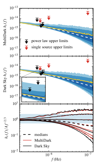
Figure 6.— Scatter in the amplitude of the gwb spectrum calculated for 5,000 realizations assuming a 25 year observation time. Contours contain 68%, 95%, and 99% of all amplitudes in each frequency bin, measured from the median. Top two panels: white dashed lines show the median, and yellow solid lines show the rms amplitude. From left to right, the black upper limits represent the epta (Lentati et al., 2015), ppta (Shannon et al., 2015), and nanograv (Arzoumanian et al., 2015) upper bounds on a $2/3$ power law gwb. The red upper limits represent the epta (Babak et al., 2016), Zhu et al. (2014), and Yi et al. (2014) upper limits on single sources. Bottom panel: the contours and medians shown above, but normalized by the best fit power law for each simulation. This is the cosmic variance of the gwb around the underlying power law spectrum. The pale blue band shows the extent of the astrophysical uncertainty from Figure 5.

The increased variance with frequency is primarily a result of Equation (missing) 5: heavy binaries have much shorter lifetimes than light binaries, and all binaries spend most of their lives at low frequencies. As a result, the signal in the lowest bins is dominated by the largest binaries ($\mathcal{M}\sim 10^{9}M_{\odot}$), but they pass through higher frequencies sufficiently quickly that they are unlikely to be seen in these bins. Signals at higher frequencies are primarily due to lower mass binaries which have larger populations and live longer, but occasionally a high-mass binary will be observed. These rare events have a significantly greater amplitude than is produced by the stable population of lower mass binaries, thereby increasing the scatter in the expected amplitude.

Individual realizations of the gwb at low frequencies have a relatively smooth signal close to the $2/3$ power law, with few individually resolvable sources. This is related to our choice of initial conditions for the binaries. Binaries are assumed to have initially circular orbits, with initial frequencies consistently chosen outside the observation window. These assumptions are required to derive a power law behavior as in Phinney (2001). However, in the real universe, smbbhs will likely have some initial eccentricity before circularizing, and the mechanism used to solve the final parsec problem may move the black holes to higher frequencies than we have assumed. Other astrophysical effects may also change the behavior of binaries at low frequencies, likely leading to a decrease in total signal. Calculations that take these factors into consideration (e.g. Enoki & Nagashima, 2007; Kocsis & Sesana, 2011; Sesana, 2013a; Ravi et al., 2014) generally see a significant departure from power-law behavior at low frequencies.

At higher frequencies the spectrum may vary significantly from bin to bin and will generally fall below the $2/3$ power law, but with some spikes rising above it. Individually resolvable sources are more likely to be observed—note that the contour for the brightest $2.5\%$ of sources at $10^{-7}$ Hz is a factor of 2 higher than the rms power law and a factor of 5 above the median.

Additionally, evolving binaries become more frequent at high frequencies. Binaries whose observed frequencies evolve through multiple bins over the course of the observation are rare events. Since this can occur only near the end of the binary’s lifetime, evolving binaries can be bright and represent a class of potentially resolvable events. Sources that experience significant evolution produce a $2/3$ power law spectrum over the period of observations for the same reason as the overall population: although the amplitude of the signal increases as $f^{2/3}$, the time spent in each bin goes as $\sqrt{f^{-8/3}}$. At frequencies $\gtrsim 50$ nHz for observations $\gtrsim 10$ years, evolving binaries dominate the bright end of the space of possible amplitudes, and help ensure the power law behavior of the rms signal.

In addition to searching for a power-law background, pta searches for individual (continuous wave) sources have been made (Jenet et al., 2004; Yardley et al., 2010; Arzoumanian et al., 2014; Zhu et al., 2014; Yi et al., 2014; Babak et al., 2016). At low frequencies, the strongest constraints are due to Babak et al. (2016), whose most robust $95\%$ upper limit on the strain amplitude is $h_{c}=9\times 10^{-15}$ at a frequency of 6 nHz. This is within a factor of 2 of our $99\%$ upper limit and roughly a factor of 3 of our median or rms amplitude for both simulations. At high frequencies, Yi et al. (2014) put upper limits on individual sources using high cadence observations of a single pulsar. For randomly located sources, their upper limit on the strain amplitude is $h_{c}=1.53\times 10^{-11}$ at $10^{-7}$ Hz, which is 4 orders of magnitude higher than our $99\%$ upper limits. The constraint on optimally located sources improves to $h_{c}=4.99\times 10^{-14}$, although this remains more than an order of magnitude higher than our $99\%$ upper limits.

The probability distribution of the cosmic variance within a single frequency bin is non-Gaussian, agreeing with the conclusions of Ravi et al. (2012) and Cornish & Sesana (2013). This can be seen clearly in Figure 6 and Figure 7, where a tail to high frequencies is readily apparent. Indeed, from Equation (missing) 15, the distribution of the power in each frequency bin is given by the sum of Poisson distributions, where each distribution is scaled by $h^{2}\propto\mathcal{M}^{10/3}$. Sources drawn from the tails of these distributions will therefore dominate the signal in that frequency bin.

As discussed in Sesana et al. (2008), the exact shape of the median signal depends on the smbbh mass function. Similarly, the amount of scatter in the amplitude at different frequency bins between possible realizations of the gwb will be sensitive to the relative quantities of smbbh of different masses. In particular, the highest-mass binaries produce the strongest signal, but are extremely rare, so their relative abundance will affect the upper limits on the possible amplitudes of the signal for all frequency bins. Smaller mass bhs are much more common and have much longer lifetimes, so there should be a population of them emitting in a wide range of frequencies in any single observation. They produce vastly less signal ($h\propto\mathcal{M}^{5/3}$) than higher-mass binaries, so the lower limits on the scatter in possible amplitudes will be set by the highest-mass population of binaries commonplace in each frequency bin. This is the reason for the significant increase in scatter as frequencies increase; at a few nHz, the very largest binaries have $\mathcal{M}\sim 10^{9}M_{\odot}$, but there are also enough binaries of this size that the highest-mass binaries which are common at that frequency are only slightly smaller. Near 100 nHz, the largest binaries have $\mathcal{M}\gtrsim 10^{8}M_{\odot}$ ($\mathcal{M}\sim 10^{9}M_{\odot}$ binaries are uncommon enough that they will rarely be seen at these frequencies), but the floor is produced by binaries with $\mathcal{M}\sim 10^{7}M_{\odot}$–$10^{8}M_{\odot}$.

The dependence of the floor on the largest commonplace population of binaries can be seen by comparing the lower bounds at high frequencies for the two simulations in Figure 6, along with the median in the Graham (2012) model in Figure 5. The latter two show a noticeable drop at frequencies of a few $\times 10^{-8}$ Hz, whereas the fiducial MultiDark model shows a more gentle decline. Although their mass functions are similar overall, MultiDark has more binaries at the lowest masses than Dark Sky. Similarly, the Graham (2012) broken power law $M_{\text{BH}}$–$M_{\text{bulge}}$ model naturally leads to a smaller population of moderate mass binaries (and subsequently more low mass binaries) than our fiducial model. The missing binaries lead to a calculated gwb with bins at high frequencies where binaries of moderate masses that should be commonplace are instead relatively rare. At these frequencies, the lower limits on the scatter in amplitude will decrease significantly. A similar, but milder effect is behind the downward turn of the $95\%$ and $99\%$ lower limits in MultiDark near $3\times 10^{-8}$ Hz. This situation is unphysical: we are unable to accurately model binaries with $\mathcal{M}<10^{8}M_{\odot}$, which are the binaries that we expect to define the floor of the scatter in the gwb at high frequencies. We therefore expect less scatter to low strain than predicted by Figure 6.

This argument only applies to the lower bounds, since the population producing the ceiling on the scatter in the gwb is well-defined. It is unlikely that even a significant population of missing lower-mass binaries would be able to affect the upper bounds; a binary at $z=0.1$ with $\mathcal{M}=10^{7}M_{\odot}$ would only add a strain of $h_{c}\sim 10^{-17}$ to a frequency bin at $10^{-7}$ Hz. Since Equation (missing) 15 varies as $\sqrt{n}$, it would take $\sim 100$ such missing binaries per frequency bin in every realization of the gwb to affect the median amplitude. A few missing binaries in each bin near $10^{-7}$ Hz in every realization, however, could bring the lower contours of Dark Sky into agreement with MultiDark. The effect of smaller binaries is even further reduced. A similar binary with $\mathcal{M}=10^{6}M_{\odot}$ would produce a strain of $h_{c}\sim 10^{-19}$, which means that $10^{4}$ such sources would be required to have the same effect as a single binary with $\mathcal{M}=10^{7}M_{\odot}$.

3.4. Effect of bin size on scatter

Thus far we have assumed a fixed set of frequency bins for all our calculations. This is of little importance for the calculation of the expected amplitude, but is not negligible when considering the scatter between realizations. We repeat our calculations of the cosmic variance for MultiDark with a fiducial set of astrophysical parameters, but assuming different total observation period $T_{\text{obs}}$, and therefore a different frequency bin width $\Delta f=1/T_{\text{obs}}$. Results are shown in Figure 7.

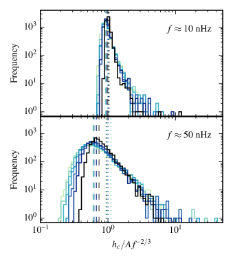
Figure 7.— The cosmic variance shown at two different frequencies, calculated assuming different bin sizes. From dark to light, histograms represent $\Delta f=1/5$ yr, $1/10$ yr, $1/15$ yr, $1/25$ yr, $1/30$ yr, $1/35$ yr. Dashed lines show the median and dotted lines show the rms amplitudes for each histogram.

As $T_{\text{obs}}$ increases ($\Delta f$ decreases), the distributions broaden. The broadening is most obvious to lower amplitudes (away from the tail), but the high-amplitude tails become broader as well. This is unsurprising, given that the original source of this scatter is Poisson noise in the smbbh mass functions. Narrower frequency bins will have fewer sources per bin, so the relative Poisson noise increases. This is quite similar to the broadening of the distribution from low frequencies to high frequencies discussed in Section 3.3. The rms amplitude remains approximately the same, since, as shown in Equation (missing) 15, the characteristic amplitude is normalized by bin width, which is a proxy for the expected number of sources per bin.

Additionally, at frequencies near 100 nHz evolving sources begin to be important for spectra calculated with long observation times (narrow frequency bins). The effect is to induce a correlation between neighboring bins. Sources that move through many bins produce local $2/3$ power law spectra. This in turn leads to a leveling of the cosmic variance contours, as can be seen in the third panel of Figure 6 at frequencies $\gtrsim 70$ nHz. Since longer observation times and narrower frequency bins allow the evolution of more sources to be observed, this effect increases with longer $T_{\text{obs}}$, but it remains unimportant at low frequencies for all observation times discussed.

4. Conclusion

We have used recent large-scale N-body simulations along with empirically calibrated scaling relations between dark matter halos and galaxies and between galaxy bulges and central black holes to calculate the expected gwb at low frequencies. This approach is complementary to the recent calculations of the gwb based on empirical galaxy merger rates. It also allows comparison with similar calculations based on the Millennium simulation, which is now over a decade old. Our calculations of the gwb have only dealt with the sky-averaged signal, but can be readily extended to create mock sky maps encompassing direction and polarization information. Such maps could be used to explore signal recovery by simulated ptas.

We have calculated the amplitude of the canonical $2/3$ power law GW spectrum to be $\log A=-15.2^{+0.4}_{-0.2}$, where the error represents the range of our variant astrophysical models and is not a $1\sigma$ Gaussian error. As shown in Figure 4, this range is consistent with amplitudes proposed by recent empirically-based calculations (Sesana, 2013b; Ravi et al., 2015). Our central amplitude is at the $3\sigma$ lower limits of the McWilliams et al. (2014) model, which assumes a high merger rate at low redshifts in order to reproduce the supermassive black hole mass function with mass growth through black hole mergers. Our model is also inconsistent with that of Kulier et al. (2015), which is calculated from hydrodynamical simulations of a galaxy cluster and a void. These works make different assumptions about merger rates of galaxies, leading to the discrepant amplitudes and highlighting the strong dependence of the signal on astrophysical effects that are only beginning to be explored.

We have estimated the uncertainty in the amplitude of the gravitational wave spectrum due to our incomplete understanding of the astrophysical effects involved. In particular, we investigated the halo mass–stellar mass relation, the $z=0$ and evolving black hole mass–stellar bulge mass, and the effect of a maximal model for the stellar bulge mass. The resulting range of amplitudes varies from our original model by a factor of $\sim 2$, and the shape of the spectrum remains essentially unchanged. We also verified that the difference in amplitude produced by independent simulations assuming different recent cosmological parameters sets is much smaller than the variance due to astrophysical uncertainties. This range in amplitude has already been constrained by the recent ppta (Shannon et al., 2015) and nanograv results (Arzoumanian et al., 2015), ruling out power law amplitudes within a factor of two above our fiducial model.

We have also characterized the scatter in amplitude expected for a single realization of the gwb. This scatter represents a fundamental uncertainty in the amplitude expected in each frequency bin due to shot noise in the source population and the fact that only a single realization of the gwb can be observed. As a result, the observed gwb will not follow a power law at all frequencies. At frequencies $\gtrsim 20$ nHz, the median amplitude becomes considerably lower than the power-law rms amplitude, with large scatter, suggesting that the gwb on average should be much harder to observe at these high frequencies. However, rare bright sources also bring the signal in the corresponding frequency bins well above the $2/3$ power-law amplitude, so it might be possible to find individual sources at high frequencies.

The two forms of uncertainty on the gwb investigated here—astrophysical and scatter between individual realizations—are fundamentally different. Astrophysical uncertainty reflects our imperfect knowledge of the physics involved, and produces a systematic change in the amplitude of the gwb, without significantly affecting the underlying power-law shape of the spectrum. On the other hand, the scatter between individual realizations of the gwb is fundamental, much like cosmic variance in the study of the cosmic microwave background power spectrum. Its presence will limit the degree to which the ‘true’ underlying amplitude and shape of the gwb can be reconstructed, even with precise measurements. In contrast with the astrophysical uncertainty, the scatter between realizations is strongly frequency dependent. As a result, we can expect that the dominant uncertainty at frequencies $\lesssim 10$ nHz is astrophysical, and any single realization of the spectrum should look close to a power law at these frequencies, although this becomes less true as observation times lengthen and frequency bins narrow.

One class of astrophysical uncertainties retains the potential to muddy this distinction. Mechanisms that allow the final parsec problem to be solved may continue to produce environmental effects on binaries that are in the process of emitting gravitational radiation. This affects the rate at which the orbits decay, typically suppressing the low-frequency amplitude of the gwb (Kocsis & Sesana, 2011; Sesana, 2013a; Ravi et al., 2014). Such environmental effects change the number of binaries common at a given separation, as would the presence of stalled binaries, potentially affecting the scatter in the amplitude, and depressing the low-frequency end of the gwb below the nearly power-law behavior shown in Figure 6. As previously shown by e.g. Ravi et al. (2014); Enoki & Nagashima (2007), another possible environmental effect is increased eccentricity at wide separations, which suppresses the low-frequency gwb since eccentric binaries emit gravitational radiation in a series of harmonics rather than at a single frequency.

Such effects would not only affect the amplitude of the gwb, but would also change its underlying form away from a power law, and would likely increase the scatter between individual realizations at low frequencies. In this case, the separation of the spectrum into a power law frequency band, where astrophysical uncertainties dominate, and a shot noise-dominated band may be complicated. There are three potential scenarios:

• The first is our default assumption in this paper and that made by most pta searches: all energy and angular momentum loss is due to gravitational wave emission and binaries are circular. The spectrum will separate into power law and shot noise-dominated regions.

• The second is of particular interest in studying the final parsec problem. In this scenario, binaries may be elliptical and the binary may lose energy and angular momentum due to processes other than gravitational wave emission, but only at the lowest frequencies measured. The spectrum would then be composed of non-power law behavior or increased scatter at the lowest frequencies, the standard power law at moderate frequencies, and shot noise at the highest frequencies.

• In the third scenario, the effects of ellipticity or other processes continue well into band, resulting in the absence of a clear power law region. This scenario would likely produce spectra that are more difficult to measure and analyze, since they are likely to be noisy and have a low amplitude at all frequencies.

Once gravitational radiation in the nHz regime has been detected, measuring its spectrum will be of much interest. We find that the effects of Poisson statistics dominate the uncertainties at the high frequency ($\gtrsim 20$ nHz) regime, while the astrophysical uncertainties dominate at lower frequencies. The solution to the final parsec problem will be encoded into the shape of the spectrum of the stochastic gwb, but the recovery of its underlying form from the measured spectrum may require characterization of the astrophysical uncertainties and an understanding of the effects of cosmic variance in the gravitational wave background.

References

- Arzoumanian et al. (2014) Arzoumanian, Z., Brazier, A., Burke-Spolaor, S., et al. 2014, ApJ, 794, 141
- Arzoumanian et al. (2015) —. 2015, arXiv:1508.03024
- Babak et al. (2016) Babak, S., Petiteau, A., Sesana, A., et al. 2016, MNRAS, 455, 1665
- Begelman et al. (1980) Begelman, M. C., Blandford, R. D., & Rees, M. J. 1980, Nature, 287, 307
- Behroozi et al. (2013a) Behroozi, P. S., Wechsler, R. H., & Conroy, C. 2013a, ApJ, 770, 57
- Behroozi et al. (2013c) Behroozi, P. S., Wechsler, R. H., & Wu, H.-Y. 2013c, ApJ, 762, 109
- Behroozi et al. (2013b) Behroozi, P. S., Wechsler, R. H., Wu, H.-Y., et al. 2013b, ApJ, 763, 18
- Bennert et al. (2010) Bennert, V. N., Treu, T., Woo, J.-H., et al. 2010, ApJ, 708, 1507
- Boylan-Kolchin et al. (2008) Boylan-Kolchin, M., Ma, C.-P., & Quataert, E. 2008, MNRAS, 383, 93
- Chandrasekhar (1943) Chandrasekhar, S. 1943, ApJ, 97, 255
- Cornish & Sesana (2013) Cornish, N. J., & Sesana, A. 2013, Classical and Quantum Gravity, 30, 224005
- Cutler & Flanagan (1994) Cutler, C., & Flanagan, É. E. 1994, Phys. Rev. D, 49, 2658
- Dotti et al. (2007) Dotti, M., Colpi, M., Haardt, F., & Mayer, L. 2007, MNRAS, 379, 956
- Dressler (1980) Dressler, A. 1980, ApJ, 236, 351
- Enoki et al. (2004) Enoki, M., Inoue, K. T., Nagashima, M., & Sugiyama, N. 2004, ApJ, 615, 19
- Enoki & Nagashima (2007) Enoki, M., & Nagashima, M. 2007, Prog. Theor. Phys., 117, 241
- Foster & Backer (1990) Foster, R. S., & Backer, D. C. 1990, ApJ, 361, 300
- Gebhardt et al. (2011) Gebhardt, K., Adams, J., Richstone, D., et al. 2011, ApJ, 729, 119
- Graham (2012) Graham, A. W. 2012, ApJ, 746, 113
- Hellings & Downs (1983) Hellings, R. W., & Downs, G. S. 1983, ApJ, 265, L39
- Hinshaw et al. (2013) Hinshaw, G., Larson, D., Komatsu, E., et al. 2013, ApJS, 208, 19
- Hlavacek-Larrondo et al. (2012) Hlavacek-Larrondo, J., Fabian, A. C., Edge, A. C., & Hogan, M. T. 2012, MNRAS, 424, 224
- Hoyle et al. (2012) Hoyle, B., Masters, K. L., Nichol, R. C., Jimenez, R., & Bamford, S. P. 2012, MNRAS, 423, 3478
- Hughes (2002) Hughes, S. A. 2002, MNRAS, 331, 805
- Jaffe & Backer (2003) Jaffe, A. H., & Backer, D. C. 2003, ApJ, 583, 616
- Jenet et al. (2004) Jenet, F. A., Lommen, A., Larson, S. L., & Wen, L. 2004, ApJ, 606, 799
- Klypin et al. (2011) Klypin, A. A., Trujillo-Gomez, S., & Primack, J. 2011, ApJ, 740, 102
- Kocsis & Sesana (2011) Kocsis, B., & Sesana, A. 2011, MNRAS, 411, 1467
- Komatsu et al. (2009) Komatsu, E., Dunkley, J., Nolta, M. R., et al. 2009, ApJS, 180, 330
- Kormendy & Ho (2013) Kormendy, J., & Ho, L. C. 2013, ARA&A, 51, 511
- Kormendy & Richstone (1995) Kormendy, J., & Richstone, D. 1995, ARA&A, 33, 581
- Kulier et al. (2015) Kulier, A., Ostriker, J. P., Natarajan, P., Lackner, C. N., & Cen, R. 2015, ApJ, 799, 178
- Lang et al. (2014) Lang, P., Wuyts, S., Somerville, R. S., et al. 2014, ApJ, 788, 11
- Lauer et al. (2007) Lauer, T. R., Faber, S. M., Richstone, D., et al. 2007, ApJ, 662, 808
- Lentati et al. (2015) Lentati, L., Taylor, S. R., Mingarelli, C. M. F., et al. 2015, MNRAS, 453, 2576
- Lotz et al. (2011) Lotz, J. M., Jonsson, P., Cox, T. J., et al. 2011, ApJ, 742, 103
- Maggiore (2008) Maggiore, M. 2008, Gravitational Waves, Vol. 1 (Oxford University Press)
- McConnell & Ma (2013) McConnell, N. J., & Ma, C.-P. 2013, ApJ, 764, 184
- McConnell et al. (2012) McConnell, N. J., Ma, C.-P., Murphy, J. D., et al. 2012, ApJ, 756, 179
- McWilliams et al. (2014) McWilliams, S. T., Ostriker, J. P., & Pretorius, F. 2014, ApJ, 789, 156
- Merritt & Milosavljević (2005) Merritt, D., & Milosavljević, M. 2005, Living Rev. Relativity, 8, 8
- Moustakas et al. (2013) Moustakas, J., Coil, A. L., Aird, J., et al. 2013, ApJ, 767, 50
- Peters & Mathews (1963) Peters, P. C., & Mathews, J. 1963, Phys. Rev., 131, 435
- Phinney (2001) Phinney, E. S. 2001, arXiv:astro-ph/0108028
- Planck Collaboration XVI (2014) Planck Collaboration XVI. 2014, A&A, 571, A16
- Prada et al. (2012) Prada, F., Klypin, A. A., Cuesta, A. J., Betancort-Rijo, J. E., & Primack, J. 2012, MNRAS, 423, 3018
- Quinlan (1996) Quinlan, G. D. 1996, New Astron., 1, 35
- Rajagopal & Romani (1995) Rajagopal, M., & Romani, R. W. 1995, ApJ, 446, 543
- Ravi et al. (2012) Ravi, V., Wyithe, J. S. B., Hobbs, G., et al. 2012, ApJ, 761, 84
- Ravi et al. (2015) Ravi, V., Wyithe, J. S. B., Shannon, R. M., & Hobbs, G. 2015, MNRAS, 447, 2772
- Ravi et al. (2014) Ravi, V., Wyithe, J. S. B., Shannon, R. M., Hobbs, G., & Manchester, R. N. 2014, MNRAS, 442, 56
- Riebe et al. (2011) Riebe, K., Partl, A. M., Enke, H., et al. 2011, arXiv:1109.0003
- Rosado (2011) Rosado, P. A. 2011, Phys. Rev. D, 84, 084004
- Rosado et al. (2015) Rosado, P. A., Sesana, A., & Gair, J. 2015, MNRAS, 451, 2417
- Rusli et al. (2013) Rusli, S. P., Thomas, J., Saglia, R. P., et al. 2013, AJ, 146, 45
- Sesana (2013a) Sesana, A. 2013a, Class. Quantum Grav., 30, 224014
- Sesana (2013b) —. 2013b, MNRAS, 433, L1
- Sesana et al. (2004) Sesana, A., Haardt, F., Madau, P., & Volonteri, M. 2004, ApJ, 611, 623
- Sesana et al. (2008) Sesana, A., Vecchio, A., & Colacino, C. N. 2008, MNRAS, 390, 192
- Sesana et al. (2009) Sesana, A., Vecchio, A., & Volonteri, M. 2009, MNRAS, 394, 2255
- Shannon et al. (2015) Shannon, R. M., Ravi, V., Lentati, L. T., et al. 2015, Science, 349, 1522
- Springel et al. (2005) Springel, V., White, S. D. M., Jenkins, A., et al. 2005, Nature, 435, 629
- Thorne (1987) Thorne, K. S. 1987, in Three Hundred Years of Gravitation, ed. S. W. Hawking & W. Israel (Cambridge University Press)
- Warren (2013) Warren, M. S. 2013, in Proceedings of SC ’13 (New York, NY, USA: ACM), 72:1
- Wilman & Erwin (2012) Wilman, D. J., & Erwin, P. 2012, ApJ, 746, 160
- Wyithe & Loeb (2003) Wyithe, J. S. B., & Loeb, A. 2003, ApJ, 590, 691
- Yardley et al. (2010) Yardley, D. R. B., Hobbs, G. B., Jenet, F. A., et al. 2010, MNRAS, 407, 669
- Yi et al. (2014) Yi, S., Stappers, B. W., Sanidas, S. A., et al. 2014, MNRAS, 445, 1245
- Zhu et al. (2014) Zhu, X.-J., Hobbs, G., Wen, L., et al. 2014, MNRAS, 444, 3709