Analysis of Jeans Instability from the Boltzmann Equation

Abstract

The dynamics of self-gravitating fluids is analyzed within the framework of a collisionless Boltzmann equation in the presence of gravitational fields and Poisson equation. Two cases are analyzed: a system with baryonic and dark matter in a static universe and a single system in an expanding universe. The amplitudes of the perturbed distribution functions are considered as a linear combination of the collision invariants of the Boltzmann equation. For the system of baryonic and dark matter, the Jeans mass of the combined system is smaller than the one of the single system indicating that a smaller mass is needed to initiate the collapse. For the single system in an expanding universe it is not necessary to make use of Jeans ”swindle”and it shown that for small wavelengths the density contrast oscillates while for large wavelengths it grows with time and the Jeans instability emerges.

1 Introduction

The search for structure formation from gas clouds is an old subject that goes back to 1902 when Jeans [1] used the system of phenomenological equations of mass and momentum densities together with the Poisson equation and showed that small perturbations in the mass density, pressure, velocity and gravitational potential in a static background with wavenumber smaller than the Jeans wavenumber could evolve with time. In terms of balance of forces the fluctuations can grow in time if the inwards directed gravitational force is larger than the outwards directed internal pressure of the gas.

Jeans theory describes the gravitational instability of self-gravitating systems by searching for conditions that small perturbations can grow and leads to a collapse of the system [2, 3, 4, 5, 6, 8, 9, 10]. It was formulated before the knowledge of the Universe expansion and one has to take into account the Jeans “swindle”, which imposes that the Poisson equation is valid only for the perturbations, since the background solution of constant mass density, pressure, gravitational potential and vanishing velocity satisfy the balance equations of mass and momentum densities, but not the Poisson equation.

The analysis of the small perturbations by using the same phenomenological equations of Jeans but taking into account the expansion of the Universe was due to Bonnor [7] in 1957. The background solutions in this case satisfy the balance equations of mass and momentum densities and Poisson equation. In this context there is no necessity to invoke Jeans “swindle” (see e.g. [2, 4, 7]).

Another way to examine Jeans instability is to consider the system of equations composed by the Newtonian version of the Boltzmann equation and Poisson equation (see e.g. [4, 5, 11, 12, 13, 14]). In these works it is considered a static Universe and Jeans “swindle”. The dispersion relation follows by taking into account small perturbations of the equilibrium values of the distribution function and gravitational potential.

Today it is well known that the matter content of the Universe is composed by baryonic matter which comprises atoms of all categories and dark matter which does not emit or interact with electromagnetic radiation. The ratio baryonic matter to dark matter estimated is about one to five. Dark matter plays a key role in structure formation because it feels only the force of gravity: the gravitational Jeans instability which allows compact structures to form is not opposed by any force, such as radiation pressure. As a result, dark matter begins to collapse into a complex network of dark matter halos well before ordinary matter, which is impeded by pressure forces. Without dark matter, the epoch of galaxy formation would occur substantially later in the universe than is observed.

The aim of this work is to obtain the collapse criterion from the Newtonian version of the Boltzmann equation and Poisson equation for a system of baryonic matter and dark matter and for a single system in an expanding spatially flat Universe. In both cases the amplitudes of the perturbed distribution functions are taken as a linear combination of the collision invariants of the Boltzmann equation. For the system of baryonic and dark matter it is shown that the mass needed to initiate the collapse is smaller than the one of a single constituent and that the ratio of the dispersion velocities have a significant role in the structure formation. For the single system the equilibrium distribution function is written in a comoving frame which takes into account Hubble’s law. Furthermore, the mass density is a solution the Friedmann and acceleration equations for a pressureless fluid. There is no necessity to use Jeans “swindle”, since the equilibrium distribution function and gravitational potential satisfy both the Boltzmann and Poisson equations. For this case the Jeans instability is connected with the growth of the density contrast for large wavelengths, which is a parameter related with the local increase of matter density.

2 Basic equations

In the phase space spanned by the space and velocity coordinates $(\mathbf{r},\mathbf{v})$ a state of a non-relativistic gas is characterized by the one-particle distribution function $f\equiv f(\mathbf{r},\mathbf{v},t)$, such that $f(\mathbf{r},\mathbf{v},t)d^{3}rd^{3}v$ gives the number of the particles in the volume element $d^{3}r$ about the position $\mathbf{r}$ and with velocity in the range $d^{3}v$ about $\mathbf{v}$. The Boltzmann equation governs the space-time evolution of the one-particle distribution function $f$ in the phase space. In the presence of a gravitational potential $\Phi$ and in the absence of collisions between the particles, the Boltzmann equation is given by (see e.g. [16, 15])

$$\partial_{t}f+\mathbf{v}\cdot\nabla f-\nabla\Phi\cdot\partial_{\mathbf{v}}f=0.$$ (1)

Here the force per unit mass which acts on a particle is only of gravitational nature ${\bf F}=-\nabla\Phi$.

The Boltzmann equation (1) follows also from a relativistic version of it in the presence of gravitational fields, where a one-particle distribution function $f\equiv f(\mathbf{r},\mathbf{p},t)$ in the phase space spanned by the space coordinates and momenta $(\mathbf{r},\mathbf{p})$ satisfies the Boltzmann equation (see e.g. [17])

$$p^{\mu}\partial_{\mu}f-\Gamma_{\mu\nu}^{i}p^{\mu}p^{\nu}\partial_{p^{i}}f=0.$$ (2)

Above the mass-shell condition $p^{\mu}p_{\mu}=m^{2}c^{2}$ – with $m$ denoting the particle rest mass – was considered. In the non-relativistic Newtonian limiting case $p^{0}\rightarrow mc$, $\mathbf{p}\rightarrow m\mathbf{v}$ and the Christoffel symbol $\Gamma_{00}^{i}\rightarrow\nabla^{i}\Phi/c^{2}$ so that (2) reduces to (1).

The connection of the gravitational potential with the one-particle distribution function is given by Poisson equation

$$\nabla^{2}\Phi=4\pi G\rho=4\pi G\int mfd^{3}v,$$ (3)

where $G$ denotes the gravitational constant and $\rho$ is the mass density of the fluid.

The analysis of cosmological problems is based on the cosmological principle which states that the Universe at large scales is spatially homogeneous and isotropic. The metric which satisfies this principle is the Friedmann-Lamaître-Robertson-Walker metric. For a spatially flat Universe the line element in this metric is written as $ds^{2}=(cdt)^{2}-a(t)^{2}\left(dx^{2}+dy^{2}+dz^{2}\right),$ where $a(t)$ is the cosmic scale factor.

Einstein’s field equations for a Universe dominated by a perfect fluid reduce to two coupled differential equations (see e.g. [2, 3, 4])

$$\left(\frac{\dot{a}}{a}\right)^{2}=\frac{8\pi G}{3}\rho,\qquad\frac{\ddot{a}}{a}=-\frac{4\pi G}{3}\left(\rho+\frac{p}{c^{2}}\right),$$ (4)

which are known as the Friedmann and acceleration equations, respectively. Above the dot denotes the derivative with respect to time and $\rho,p$ are the mass density and the pressure of the sources of the gravitational field, respectively.

In this work we are interested in matter dominated Universe, where the sources of the gravitational field are pressureless $p=0$. In this case equations (4) can be solved for the mass density as a function of the cosmic scale factor, yielding

$$\rho=\rho_{0}\left(\frac{a_{0}}{a}\right)^{3},$$ (5)

where $\rho_{0}$ and $a_{0}$ are the values of the mass density and cosmic scale factor at $t=0$, respectively.

Another relationship which will be used below is Hubble’s law $\dot{\mathbf{r}}=(\dot{a}/a)\mathbf{r}$ which relates the recession velocity of an object $\dot{\mathbf{r}}$ with its physical distance $\mathbf{r}$ in an expanding Universe. The quantity $H=\dot{a}/a$ is known as Hubble parameter.

3 Jeans instability for systems of one component

We start by analyzing the Jeans instability for systems with one component. This subject was discussed in some books, see e.g. [4, 5], but here a new methodology is introduced, which is based on the collision invariants of the Boltzmann equation [15]. The collisionless Boltzmann (1) and Poisson (3) equations imply a coupled system of equations for the distribution function $f(\mathbf{r},\mathbf{v},t)$ and gravitational potential $\Phi(\mathbf{r},t)$, which we reproduce below:

$$\partial_{t}f+\mathbf{v}\cdot\nabla f-\nabla\Phi\cdot\partial_{\mathbf{v}}f=0,\qquad\nabla^{2}\Phi=4\pi G\int mfd^{3}v.$$ (6)

At equilibrium the distribution function and the gravitational potential of a self-gravitating system do not depend on time and the collisionless Boltzmann equation (6)₁ is satisfied if the distribution function depends only of the velocity of the particles $f_{0}(\mathbf{v})$ and the gravitational potential gradient vanishes $\nabla\Phi_{0}=0$. Note that the condition $\nabla\Phi_{0}=0$ may follow from symmetry considerations, because in a homogeneous system there is no preference in the direction of the gravitational potential gradient. The same restriction for the gravitational potential gradient is also considered for a system described by the balance equations of mass density and fluid velocity, since constant values of pressure and density and vanishing fluid velocity and gravitational potential gradient satisfy these equations. However, the condition $\nabla\Phi_{0}=0$ does not satisfy the Poisson equation (6)₂ due to the fact that its right-hand side refers to the mass density of the self-gravitating system. In order to remove this inconsistency one makes use of the Jeans “swindle”, which considers that the Poisson equation is valid only for the perturbed distribution function and perturbed gravitational potential.

We require that the equilibrium state is subjected to small perturbations $h(\mathbf{r},\mathbf{v},t)$ and $\Phi_{1}(\mathbf{r},t)$:

$$f(\mathbf{r},\mathbf{v},t)=f_{0}(\mathbf{v})\left[1+h(\mathbf{r},\mathbf{v},t)\right],\qquad\Phi(\mathbf{r},t)=\Phi_{0}+\Phi_{1}(\mathbf{r},t).$$ (7)

The equilibrium value of the gravitational potential is considered as a constant in order to fulfill the condition $\nabla\Phi_{0}=0$ and the equilibrium distribution function is the Maxwellian one

$$f_{0}(\mathbf{v})=\frac{\rho}{m}\frac{e^{-{v^{2}}/{2\sigma^{2}}}}{(2\pi\sigma^{2})^{3/2}},$$ (8)

where $\sigma=\sqrt{kT/m}$ is the dispersion (thermal) velocity and $k$, $T$ denote the Boltzmann constant and the temperature of the system, respectively. Note that the collisionless Boltzmann equation (6)₁ is a differential equation for the distribution function and its solution depends on the problem we are analyzing. Here we are interested in analyzing disturbances which can be represented by plane waves so that we have required that the distribution function is a sum of an equilibrium distribution function plus an arbitrary function which characterizes a plane wave solution of small amplitude.

We insert the representations (7) into the Boltzmann and Poisson equations (6) and get the following system of equations for the perturbed quantities $h$ and $\Phi_{1}$:

$$f_{0}\left[\partial_{t}h+\mathbf{v}\cdot\nabla h\right]-\nabla\Phi_{1}\cdot\partial_{\mathbf{v}}f_{0}=0,\qquad\nabla^{2}\Phi_{1}=4\pi G\int mf_{0}hd^{3}v.$$ (9)

In (9)₁ we have neglected products of $\nabla\Phi_{1}$ with $h$ and $\partial_{\mathbf{v}}h$, since $h$ and $\Phi_{1}$ are supposed as small quantities. Furthermore, we have considered that the Poisson equation refers only to the perturbed values of the distribution function and gravitational potential and taken $\nabla\Phi_{0}=0$.

The perturbations $h$ and $\Phi_{1}$ are now represented by plane waves of frequency $\omega$ and wavenumber vector $\mathbf{k}$ such that

$$h(\mathbf{r},\mathbf{v},t)=h_{1}(\mathbf{v})\exp\left[i\left(\mathbf{k}\cdot\mathbf{r}-\omega t\right)\right],\qquad\Phi_{1}(\mathbf{r},t)=\phi\exp\left[i\left(\mathbf{k}\cdot\mathbf{r}-\omega t\right)\right].$$ (10)

In the above equations $\phi$ is a constant amplitude while $h_{1}(\mathbf{v})$ is given as a combination of the collision invariants of the Boltzmann equation, namely: 1, $\mathbf{v}$ and $\mathbf{v}^{2}$ (see e.g. [15, 16]). Its expression is written as

$$h_{1}(\mathbf{v})=A+\mathbf{B}\cdot\mathbf{v}+D\mathbf{v}^{2},$$ (11)

where $A$, $\bf B$ and $D$ are unknown constants.

The insertion of (10) and (11) together with (8) into the perturbed Boltzmann and Poisson equations (9) lead to

$$\left(A+\mathbf{B}\cdot\mathbf{v}+D\mathbf{v}^{2}\right)\left[\omega-\mathbf{k}\cdot\mathbf{v}\right]-\mathbf{k}\cdot\mathbf{v}\frac{\phi}{\sigma^{2}}=0,\qquad\textsf{k}^{2}\phi+4\pi G\left(A+3\sigma^{2}D\right)\rho=0,$$ (12)

where $\textsf{k}=|\mathbf{k}|$.

Now a system of equations for $A$, $B=\bf B\cdot k$, $D$ and $\phi$ can be obtained from the multiplication of (12)₁ by the collision invariants $\left(1,\mathbf{v},\mathbf{v}^{2}\right)$ and integration of the resulting equations, yielding

$$\omega\left(A+3\sigma^{2}D\right)-\sigma^{2}B=0,\qquad\omega B-\left[A+5\sigma^{2}D+\frac{\phi}{\sigma^{2}}\right]\textsf{k}^{2}=0,\qquad\omega\left(3A+15\sigma^{2}D\right)-5\sigma^{2}B=0.$$ (13)

The system of equations (13) together with (12)₂ has a non-trivial solution if the determinant of the coefficients $A$, $B$, $D$ and $\phi$ vanishes, which implies the dispersion relation:

$$\omega_{*}\left(1-\textsf{k}_{*}^{2}+\omega_{*}^{2}\right)=0.$$ (14)

Above the dimensionless wavenumber modulus $\textsf{k}_{*}$ and frequency $\omega_{*}$ are given by the relationships

$$\textsf{k}_{*}=\frac{v_{s}\textsf{k}}{\sqrt{4\pi G\rho}}=\frac{\textsf{k}}{\textsf{k}_{J}},\qquad\omega_{*}=\frac{\omega}{\sqrt{4\pi G\rho}}.$$ (15)

Here we have introduced the adiabatic sound speed $v_{s}=\sqrt{5/3}\,\sigma$ and the Jeans wavenumber $\textsf{k}_{J}=\sqrt{4\pi G\rho}/v_{s}$.

We have the following solutions for the dimensionless frequency from the dispersion relation (14): $\omega_{*}=0$ and

$$\omega_{*}=\pm\sqrt{\frac{\textsf{k}^{2}}{\textsf{k}_{J}^{2}}-1}.$$ (16)

From the above equation we may infer that for $\textsf{k}>\textsf{k}_{J}$ (small wavelengths), $\omega_{*}$ is a real quantity and the perturbations – due to the factor $\exp\left(-i\omega t\right)$ – will propagate as harmonic waves in time. However, if $\textsf{k}<\textsf{k}_{J}$ (big wavelengths), $\omega_{*}$ is a pure imaginary quantity and one of the perturbations will grow with time, while the other will decay with time. The perturbation which grows with time is associated with Jeans instability.

A very simple model is described in the literature to understand the Jeans instability. Consider a mass $M$ enclosed in a spherical volume of radius $\lambda$ in which there exists a mass density inhomogeneity. This inhomogeneity will grow if the gravity force $F_{G}$ per unit mass is greater than the opposed pressure force $F_{P}$ per unit of mass, i.e.,

$$F_{G}=\frac{GM}{\lambda^{2}}\propto\frac{G\rho\lambda^{3}}{\lambda^{2}}=G\rho\lambda>F_{P}\propto\frac{p\lambda^{2}}{\rho\lambda^{3}}\propto\frac{v_{s}^{2}}{\lambda},\qquad\hbox{since}\qquad v_{s}^{2}\propto\frac{p}{\rho}.$$ (17)

Now identifying the Jeans wavelength in terms of the Jeans wavenumber $\lambda_{J}=2\pi/\textsf{k}_{J}={2\pi v_{s}}/{\sqrt{4\pi G\rho}}$ and $\lambda=2\pi/\textsf{k}$, the inequality $\textsf{k}<\textsf{k}_{J}$ follows.

4 Jeans instability for systems with two components

In this section we shall analyze Jeans instability by taking into account two collisionless Boltzmann equations, one for the baryonic matter and another for the dark matter which are connected with the Poisson equation. We shall use the indices $b$ and $d$ for the baryonic and dark matter, respectively. The corresponding evolution equations for the distribution functions of baryonic matter $f_{b}\equiv f(\mathbf{x},\mathbf{v}_{b},t)$ and dark matter $f_{d}\equiv f(\mathbf{x},\mathbf{v}_{d},t)$ are given by the collisionless Boltzmann equations

$$\partial_{t}f_{b}+\mathbf{v}_{b}\cdot\nabla f_{b}-\nabla\Phi\cdot\partial_{\mathbf{v}_{b}}f_{b}=0,\qquad\partial_{t}f_{d}+\mathbf{v}_{d}\cdot\nabla f_{d}-\nabla\Phi\cdot\partial_{\mathbf{v}_{d}}f_{d}=0,$$ (18)

which are connected with the Poisson equation

$$\nabla^{2}\Phi=4\pi G\left(\int m_{b}f_{b}d^{3}v_{b}+\int m_{d}f_{d}d^{3}v_{d}\right)=4\pi G(\rho_{b}+\rho_{d}).$$ (19)

Above $(m_{b},m_{d})$ and $(\rho_{b},\rho_{d})$ are the masses and mass densities of the baryonic and dark matter, respectively.

Following the same methodology of the previous section we suppose that the distribution functions $f(\mathbf{x},\mathbf{v}_{b},t)$, $f(\mathbf{x},\mathbf{v}_{d},t)$ and the potential $\Phi$ are subjected to small perturbations $h_{b}(\mathbf{r},\mathbf{v}_{b},t)$, $h_{d}(\mathbf{r},\mathbf{v}_{d},t)$ and $\Phi_{1}(\mathbf{r},t)$ from their equilibrium values $f_{b}^{0}({\bf v}_{b})$, $f_{d}^{0}({\bf v}_{d})$ and $\Phi_{0}$, respectively. Hence we write

$$f(\mathbf{r},\mathbf{v}_{b},t)=f_{b}^{0}({\bf v}_{b})\left[1+h_{b}(\mathbf{r},\mathbf{v}_{b},t)\right],\qquad f(\mathbf{r},\mathbf{v}_{d},t)=f_{d}^{0}({\bf v}_{d})\left[1+h_{d}(\mathbf{r},\mathbf{v}_{d},t)\right],\qquad\Phi(\mathbf{r},t)=\Phi_{0}+\Phi_{1}(\mathbf{r},t).$$ (20)

where the equilibrium distribution functions are the Maxwellians

$$f_{b}^{0}(\mathbf{r},\mathbf{v}_{b},t)=\frac{\rho_{b}}{m_{b}}\frac{e^{-\mathbf{v}_{b}^{2}/2\sigma_{b}^{2}}}{(2\pi\sigma_{b}^{2})^{3/2}},\qquad f_{d}^{0}(\mathbf{r},\mathbf{v}_{d},t)=\frac{\rho_{d}}{m_{d}}\frac{e^{-\mathbf{v}_{d}^{2}/2\sigma_{d}^{2}}}{(2\pi\sigma_{d}^{2})^{3/2}}.$$ (21)

Here $\sigma_{b}=\sqrt{kT_{b}/m_{b}}$ and $\sigma_{d}=\sqrt{kT_{d}/m_{d}}$ are the dispersion velocities of the baryonic and dark matter which are associated with their temperatures $T_{b}$ and $T_{d}$, respectively.

From the insertion of the representations (20) into the Boltzmann (18) and Poisson (19) equations yields

$$f_{b}^{0}\left[\partial_{t}h_{b}+\mathbf{v}_{b}\cdot\nabla h_{b}\right]-\nabla\Phi_{1}\cdot\partial_{\mathbf{v}_{b}}f_{b}^{0}=0,\qquad f_{d}^{0}\left[\partial_{t}h_{d}+\mathbf{v}_{d}\cdot\nabla h_{d}\right]-\nabla\Phi_{1}\cdot\partial_{\mathbf{v}_{d}}f_{d}^{0}=0,$$ (22)

$$\nabla^{2}\Phi_{1}=4\pi G\left(\int m_{b}f_{b}^{0}h_{b}d^{3}v_{b}+\int m_{d}f_{d}^{0}h_{d}d^{3}v_{d}\right).$$ (23)

Here we followed the same methodology which was used to obtain the system of equations (9) and considered the Jeans ”swindle”.

We represent the perturbations as plane waves of frequency $\omega$ and wavenumber vector ${\bf k}$

$$h_{b}(\mathbf{r},\mathbf{v}_{b},t)=h_{b}^{1}(\mathbf{v}_{b})\exp\left(i\mathbf{k}\cdot\mathbf{r}-i\omega t\right),\quad h_{d}(\mathbf{r},\mathbf{v}_{d},t)=h_{d}^{1}(\mathbf{v}_{d})\exp\left(i\mathbf{k}\cdot\mathbf{r}-i\omega t\right),\quad\Phi_{1}(\mathbf{r},t)=\phi\exp\left(i\mathbf{k}\cdot\mathbf{r}-i\omega t\right),$$ (24)

where the amplitude $\phi$ is constant, while $h_{b}^{1}$ and $h_{d}^{1}$ are given in terms of the collision invariants of the Boltzmann equations $\left(1,\mathbf{v}_{b},\mathbf{v}_{b}^{2}\right)$ and $\left(1,\mathbf{v}_{d},\mathbf{v}_{d}^{2}\right)$:

$$h_{b}^{1}({\bf v}_{b})=A_{b}+\mathbf{B}_{b}\cdot\mathbf{v}_{b}+D_{b}\mathbf{v}_{b}^{2},\qquad h_{d}^{1}({\bf v}_{d})=A_{d}+\mathbf{B}_{d}\cdot\mathbf{v}_{d}+D_{d}\mathbf{v}_{d}^{2}.$$ (25)

Above $A_{b},A_{d},\mathbf{B}_{b},\mathbf{B}_{d},D_{b},D_{d}$ are constants

Now the insertion of (24) together with (25) and (21) into (22) and (23) leads to

$$\left(A_{\alpha}+\mathbf{B}_{\alpha}\cdot\mathbf{v}_{\alpha}+D_{\alpha}\mathbf{v}_{\alpha}^{2}\right)\left[\omega-\mathbf{k}\cdot\mathbf{v}_{\alpha}\right]-\mathbf{k}\cdot\mathbf{v}_{\alpha}\frac{\phi}{\sigma_{\alpha}^{2}}=0,\qquad\alpha=b,d$$ (26)

$$\textsf{k}^{2}\phi+4\pi G\left[\left(A_{b}+3\sigma_{b}^{2}D_{b}\right)\rho_{b}+\left(A_{d}+3\sigma_{d}^{2}D_{d}\right)\rho_{d}\right]=0.$$ (27)

In order to get a system of algebraic equations for $A_{b},A_{d},B_{b}=\mathbf{B}_{b}\cdot\mathbf{k},B_{d}=\mathbf{B}_{d}\cdot\mathbf{k},D_{b},D_{d}$ and $\phi$ we multiply (26) by the collision invariants $\left(1,\mathbf{v}_{b},\mathbf{v}_{b}^{2}\right)$ and $\left(1,\mathbf{v}_{d},\mathbf{v}_{d}^{2}\right)$, respectively, and integrate the resulting equations, yielding for $(\alpha=b,d)$

$$\omega\left(A_{\alpha}+3\sigma_{\alpha}^{2}D_{\alpha}\right)-B_{\alpha}\sigma_{\alpha}^{2}=0,\qquad\omega B_{\alpha}-\left[A_{\alpha}+5\sigma_{\alpha}^{2}D_{\alpha}+\frac{\phi}{\sigma_{\alpha}^{2}}\right]\textsf{k}^{2}=0,\qquad\omega\left(3A_{\alpha}+15\sigma_{\alpha}^{2}D_{\alpha}\right)-5B_{\alpha}\sigma_{\alpha}^{2}=0.$$ (28)

A non-trivial solution of the system of equations (27) and (28) is found if the determinant of the coefficients $A_{b},A_{d},B_{b},B_{d},D_{b},D_{d}$, $\phi$ vanishes, which implies the dispersion relation:

$$\omega_{*}^{4}+\left[1+\frac{\rho_{b}}{\rho_{d}}-\left(1+\frac{\sigma_{b}^{2}}{\sigma_{d}^{2}}\right)\textsf{k}_{*}^{2}\right]\omega_{*}^{2}+\frac{\sigma_{b}^{2}}{\sigma_{d}^{2}}\left[\textsf{k}_{*}^{2}-1-\frac{\rho_{b}\sigma_{d}^{2}}{\rho_{d}\sigma_{b}^{2}}\right]\textsf{k}_{*}^{2}=0.$$ (29)

Here we have introduced the dimensionless wavenumber $\textsf{k}_{*}$ and frequency $\omega_{*}$ defined in terms of the dark matter Jeans wavenumber $\textsf{k}_{J}^{d}=\sqrt{4\pi G\rho_{d}}/v_{s}^{d}$ – with $v_{s}^{d}=\sqrt{5/3}\,\sigma_{d}$ denoting the dark matter sound speed – since as it was explained in the introduction the dark matter begins to collapse into a complex network of dark matter halos well before ordinary matter. The dimensionless wavenumber and frequency read

$$\textsf{k}_{\ast}=\frac{\textsf{k}}{\textsf{k}_{J}^{d}}=\frac{\textsf{k}\,v_{s}^{d}}{\sqrt{4\pi G\rho_{d}}},\qquad\omega_{\ast}=\frac{\omega}{\sqrt{4\pi G\rho_{d}}}.$$ (30)

We note that the dispersion relation (29) is a function of two ratios $\rho_{d}/\rho_{b}$ and $\sigma_{d}/\sigma_{b}$. The mass density ratio $\rho_{d}/\rho_{b}$ can be associated with the present value of the density parameter ratio $\rho_{d}/\rho_{b}=\Omega_{d}/\Omega_{b}\approx 5.5$ [18], since this ratio has not changed considerably during the evolution of the universe. For the dispersion velocities ratio $\sigma_{d}/\sigma_{b}$ there is no fixed value. One value we shall use is taken from Ref. [19] where Milky Way-like galaxy simulations including both baryonic and dark matter were performed. From this work we have inferred that in one of the simulations where Maxwellian distributions are considered the ratio is given by $\sigma_{d}/\sigma_{b}=170/93\approx 1.83$.

From the dispersion relation (29) we have the following solutions for the dimensionless frequency:

$$\omega_{*} = \pm\frac{\sigma_{b}}{\sqrt{2}\sigma_{d}}\sqrt{\textsf{k}_{*}^{2}\left(1+\frac{\sigma_{d}^{2}}{\sigma_{b}^{2}}\right)-\frac{\sigma_{d}^{2}}{\sigma_{b}^{2}}\left(1+\frac{\rho_{b}}{\rho_{d}}\right)\pm\Delta},$$ (31)

$$\Delta = \sqrt{\left[\textsf{k}_{*}^{2}\left(1+\frac{\sigma_{d}^{2}}{\sigma_{b}^{2}}\right)-\frac{\sigma_{d}^{2}}{\sigma_{b}^{2}}\left(1+\frac{\rho_{b}}{\rho_{d}}\right)\right]^{2}-4\frac{\sigma_{d}^{2}}{\sigma_{b}^{2}}\left[\textsf{k}_{*}^{4}-\left(1+\frac{\rho_{b}\sigma_{d}^{2}}{\rho_{d}\sigma_{b}^{2}}\right)\textsf{k}_{*}^{2}\right]}.$$ (32)

Without the baryonic matter, i.e. for $\rho_{b}=\sigma_{b}=0$, the dispersion relation (29) reduces to:

$$\omega_{*}^{4}+\left[1-\textsf{k}_{*}^{2}\right]\omega_{*}^{2}=0,$$ (33)

which has the solutions $\omega_{*}=0$ and $\omega_{*}=\pm\sqrt{\textsf{k}^{2}/\textsf{k}_{J}^{2}-1}$, i. e., we recover the Jeans solution for one component.

Two solutions of (31) provide real values for $\omega_{*}$ for any $\textsf{k}_{*}$ so that we have harmonic waves in time for these two solutions. However the other two solutions furnish imaginary values for $\omega_{*}$ for some values of $\textsf{k}_{*}$ so that instead of harmonic waves the amplitude of the disturbance will grow or decay. The one which grows is associated with Jeans instability. The value of $\textsf{k}_{*}$ where $\omega_{*}$ changes from the imaginary value to the real value is obtained by taking $\omega_{*}$ equal to zero in (29) and we get

$$\textsf{k}_{*}=\frac{\textsf{k}_{J}^{\rm db}}{\textsf{k}_{J}^{\rm d}}=\sqrt{1+\frac{\rho_{b}\sigma_{d}^{2}}{\rho_{d}\sigma_{b}^{2}}}=\frac{\lambda_{J}^{\rm d}}{\lambda_{J}^{\rm db}}.$$ (34)

This equation is interpreted as the ratio of two Jeans wavenumbers, the one $\textsf{k}_{J}^{\rm db}$ refers to the system dark-baryonic matter while $\textsf{k}_{J}^{\rm d}$ to the dark matter.

We can also analyze the amount of mass which is necessary to initiate the collapse, which is the Jeans mass contained in a sphere of diameter equal to the wavelength $\lambda=2\pi/\textsf{k}$. Hence, we can build the ratio of Jeans masses, one for the system dark-baryonic matter $M_{J}^{\rm db}$ and another for the dark matter alone $M_{J}^{\rm d}$, namely

$$\frac{M_{J}^{\rm db}}{M_{J}^{\rm d}}=\frac{\rho_{b}+\rho_{d}}{\rho_{d}}\left(\frac{\lambda_{J}^{\rm db}}{\lambda_{J}^{\rm d}}\right)^{3}=\left(1+\frac{\rho_{b}}{\rho_{d}}\right)\left(\sqrt{1+\frac{\rho_{b}\sigma_{d}^{2}}{\rho_{d}\sigma_{b}^{2}}}\right)^{-3}.$$ (35)

$\sigma_{d}/\sigma_{b}$	1.00	1.20	1.40	1.60	1.83	2.00	2.20
$M_{J}^{\rm db}/M_{J}^{\rm d}$	0.9199	0.8338	0.7481	0.6662	0.5791	0.5206	0.4585

Table 1: Ratio of Jeans masses $M_{J}^{\rm db}/M_{J}^{\rm d}$ as function of the ratio of the dispersion velocities $\sigma_{d}/\sigma_{b}$ for $\rho_{d}/\rho_{b}=5.5$.

In Table 1 the ratio of the Jeans masses of the system baryonic-dark matter and dark matter are given as functions of the dispersion velocities ratio for fixed values of the mass densities ratio. From this table we infer that if we increase the dispersion velocities ratio, the mass needed to begin the collapse becomes smaller in comparison with the mass where only one constituent is present. This can be understood, since when the ratio $\sigma_{d}/\sigma_{b}$ is large the dispersion velocity of the baryonic matter is smaller than the one of the dark matter and the baryonic matter hardly overcome the escape velocity of a given gravitational field.

5 Jeans instability in an expanding Universe

In this section we shall analyze Jeans instability by taking into account the collisionless Boltzmann and Poisson equations (9) but in an expanding Universe where a pressureless fluid is the source of the gravitational field.

Now the equilibrium distribution function is written in a comoving frame as

$$f_{0}(\mathbf{r},\mathbf{v},t)=\frac{\rho}{m}\frac{1}{(2\pi\sigma^{2})^{3/2}}\exp\left(-\frac{\left(\mathbf{v}-\frac{\dot{a}}{a}\mathbf{r}\right)^{2}}{2\sigma^{2}}\right),$$ (36)

thanks to Hubble’s law $\dot{\mathbf{r}}=(\dot{a}/a)\mathbf{r}$. Note that according to (5) the mass density $\rho$ is only a function of time.

The gravitational potential function

$$\Phi_{0}(\mathbf{r},t)=\frac{2\pi}{3}G\rho r^{2},$$ (37)

and the equilibrium distribution function (36) satisfy the Poisson and Boltzmann equations

$$\nabla^{2}\Phi_{0}=4\pi G\int mf_{0}d^{3}v=4\pi G\rho,\qquad\partial_{t}f_{0}+\mathbf{v}\cdot\nabla f_{0}-\nabla\Phi_{0}\cdot\partial_{\mathbf{v}}f_{0}=0,$$ (38)

by taking into account the Friedmann and acceleration equations (4) and provided that the dispersion velocity is proportional to the inverse of the cosmic scale factor and does not depend on the spatial coordinates, namely $\sigma(t)\propto 1/a(t)$.

As in the previous sections we require that the equilibrium state defined by the distribution function (36) and gravitational potential (37) is subjected to small perturbations characterized by $h(\mathbf{r},\mathbf{v},t)$ and $\Phi_{1}(\mathbf{r},t)$ such that

$$f(\mathbf{r},\mathbf{v},t)=f_{0}(\mathbf{r},\mathbf{v},t)\left[1+h(\mathbf{r},\mathbf{v},t)\right],\qquad\Phi(\mathbf{r},t)=\Phi_{0}(\mathbf{r},t)+\Phi_{1}(\mathbf{r},t).$$ (39)

Note that (39) is similar to (7), the difference between them lies in the dependence of the equilibrium distribution function and gravitational potential at equilibrium, which now are functions of the space-time coordinates.

Now the insertion of (39) into the collisionless Boltzmann and Poisson equations (6) leads the system of equations for $h$ and $\Phi_{1}$:

$$f_{0}\left[\partial_{t}h+\mathbf{v}\cdot\nabla h-\underline{\nabla\Phi_{0}\cdot\partial_{\mathbf{v}}h}\right]-\nabla\Phi_{1}\cdot\partial_{\mathbf{v}}f_{0}=0,\qquad\nabla^{2}\Phi_{1}=4\pi G\int mf_{0}hd^{3}v.$$ (40)

Note that the underlined term above does not show up in (9), since it was supposed that $\nabla\Phi_{0}=0$. Above the products of $\nabla\Phi_{1}$ with $h$ and $\partial_{\mathbf{v}}h$ were also neglected.

The perturbations $h$ and $\Phi_{1}$ represented by plane waves of wavenumber vector ${\bf q}/a(t)$, reads

$$h(\mathbf{r},\mathbf{v},t)=h_{1}(\mathbf{r},\mathbf{v},t)\exp\left(i\frac{\mathbf{q}\cdot\mathbf{r}}{a(t)}\right),\qquad\Phi_{1}(\mathbf{r},t)=\phi(t)\exp\left(i\frac{\mathbf{q}\cdot\mathbf{r}}{a(t)}\right).$$ (41)

The factor $1/a(t)$ in the wavenumber reflects the fact that the wavelength is stretched out in an expanding Universe. Here we cannot assume a harmonic wave in time, since the factors of the equations depend on time. Hence, $\phi(t)$ is an amplitude that depends on time, while $h_{1}(\mathbf{r},\mathbf{v},t)$ is given as a combination of the collision invariants of the Boltzmann equation in a comoving frame, i.e., 1, $\mathbf{v}-\frac{\dot{a}}{a}\mathbf{r}$ and $\left(\mathbf{v}-\frac{\dot{a}}{a}\mathbf{r}\right)^{2}$:

$$h_{1}(\mathbf{r},\mathbf{v},t)=A(t)+\mathbf{B}(t)\cdot\left(\mathbf{v}-\frac{\dot{a}}{a}\mathbf{r}\right)+D(t)\left(\mathbf{v}-\frac{\dot{a}}{a}\mathbf{r}\right)^{2},$$ (42)

where $A(t)$, ${\bf B}(t)$ and $D(t)$ are also functions of time.

The methodology used here is the same as in the previous sections. We insert (41) and (42) together with (36) and (37) into the perturbed Boltzmann and Poisson equations (40) and multiply the resulting equation from the Boltzmann equation by the collision invariants $\left(1,\mathbf{v}-\frac{\dot{a}}{a}\mathbf{r},\left(\mathbf{v}-\frac{\dot{a}}{a}\mathbf{r}\right)^{2}\right)$ and integrate. Hence we get the following system of differential equations:

$$\frac{dA(t)}{dt}+3\sigma^{2}\frac{dD(t)}{dt}+i\frac{\sigma^{2}}{a}B(t)-6\frac{\dot{a}}{a}\sigma^{2}D(t)=0,\qquad\frac{dB(t)}{dt}+i\frac{q^{2}}{a}\left[A(t)+5\sigma^{2}D(t)+\frac{\phi(t)}{\sigma^{2}}\right]-\frac{\dot{a}}{a}B(t)=0,\qquad$$ (43)

$$3\frac{dA(t)}{dt}+15\sigma^{2}\frac{dD(t)}{dt}+i5\frac{\sigma^{2}}{a}B(t)-30\frac{\dot{a}}{a}\sigma^{2}D(t)=0,\qquad\frac{q^{2}}{a^{2}}\phi(t)+4\pi G\left[A(t)+3\sigma^{2}D(t)\right]\rho=0.$$ (44)

Above we have introduced $B(t)=\mathbf{B}(t)\cdot\mathbf{q}$.

In galaxy formation is usual to introduce the density contrast which is a parameter that indicates where there are local increase in the matter density. It is defined by the ratio of perturbed and unperturbed mass densities $\delta_{\rho}=\overline{\rho}/\rho$. Here the density contrast reads $\delta_{\rho}=A(t)+3\sigma^{2}D(t)$, and we can obtain from the system of differential equations (43) and (44) that $A$ is a constant (say $A=1$) and the following differential equation for the density contrast

$$\tau^{2}\,\delta_{\rho}^{\prime\prime}+\frac{4}{3}\tau\,\delta_{\rho}^{\prime}-\frac{2}{3}\left(1-\frac{3\lambda_{J}^{2}}{5\lambda_{0}^{2}\tau^{\frac{2}{3}}}\right)\delta_{\rho}-\frac{4\lambda_{J}^{2}}{25\lambda_{0}^{2}\tau^{\frac{2}{3}}}=0,\qquad\hbox{where}\qquad\lambda_{0}=\frac{2\pi a_{0}}{q},\qquad\lambda_{J}=\frac{10\pi\sigma_{0}}{3\sqrt{4\pi G\rho_{0}}}.$$ (45)

In the above equation we have used the relationship $a=a_{0}(6\pi G\rho_{0}t^{2})^{1/3}$ which follows from the integration of (4). Furthermore, $\tau=t\sqrt{6\pi G\rho_{0}}$ is a dimensionless time and the primes are derivatives with respect to $\tau$. The solution of (45) is given in terms of Bessel functions of first kind $J_{\pm\frac{5}{2}}(\Lambda/\tau^{\frac{1}{3}})$ and reads

$$\delta_{\rho}=\tau^{-\frac{1}{6}}\left[C_{1}J_{\frac{5}{2}}\left(\frac{\Lambda}{\tau^{\frac{1}{3}}}\right)+C_{2}J_{-\frac{5}{2}}\left(\frac{\Lambda}{\tau^{\frac{1}{3}}}\right)\right]+\underline{\frac{2}{5}\left(1+\frac{5\tau^{\frac{2}{3}}}{3\Lambda^{2}}\right)},\qquad\hbox{where}\qquad\Lambda=\sqrt{\frac{18}{5}}\frac{\lambda_{J}}{\lambda_{0}}.$$ (46)

The solution (46) differs from the one that comes from the analysis of the balance equations for mass, momentum and entropy densities in an expanding universe (see e.g. [4]) due to the underlined term which refers to the time evolution of the density contrast in a matter dominated universe. For large values of the ratio $\lambda_{J}/\lambda_{0}$ (small wavelengths) the Bessel functions imply oscillations of the density contrast while for small values of $\lambda_{J}/\lambda_{0}$ (large wavelengths) the first term in (46) furnishes two solutions one decaying according to $1/\tau$ and another growing with $\tau^{2/3}$. However due to the underlined term with $\tau^{2/3}$ the density contrast will grow with time for small values of $\lambda_{J}/\lambda_{0}$ and this solution corresponds to Jeans instability. In Fig. 1 it is shown the time evolution of the density contrast for different values of $\Lambda$, i.e. for different values of the ratio $\lambda_{J}/\lambda_{0}$.

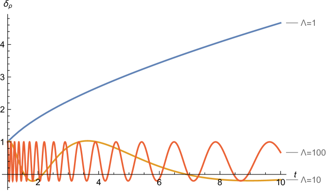
Figure 1: (color online) Density contrast $\delta_{\rho}$ as function of time $\tau$ for different values of the ratio $\Lambda=\sqrt{18/5}\lambda_{J}/\lambda_{0}$.

6 Conclusions

In this work we have analyzed Jeans instability using the collisionless Boltzmann and Poisson equations for a system of baryonic and dark matter in a static universe and a system of a single constituent in an expanding universe. For the system baryonic-dark matter the Jeans mass of the system is smaller than that of a single component indicating that the structures are formed earlier than in the latter case. Furthermore, the dispersion velocities ratio dark-matter/baryonic-matter has influence of the Jeans masses, since small dispersion velocity of the baryonic matter in comparison with the one of the dark matter implies that the baryonic matter hardly overcome the escape velocity of a given gravitational field. For the single component in an expanding Universe the background solutions for the distribution function and gravitational potential satisfy both Boltzmann and Poisson equations without the introduction of Jeans “swindle”. The equilibrium distribution function is written in a comoving frame that takes into account Hubble’s law and the mass density is a solution of Friedmann and acceleration equations for a pressureless fluid. The Jeans instability is connected with a parameter that indicates the local increase in the matter density, the so-called density contrast. It is shown that for large wavelengths the density contrast grows with time.

References

• [1] J. H. Jeans, Phil. Trans. Royal Soc. London 199, 1 (1902).
• [2] S. Weinberg, Gravitation and Cosmology, Principles and Applications of the General Theory of Relativity (John Wiley & Sons, New York, 1972).
• [3] J. A. Peacock, Cosmological Physics (Cambridge University Press, Cambridge, 1999).
• [4] P. Coles and F. Lucchin, The Origin and Evolution of Cosmic Structure, 2nd. edn., (John Wiley, Chichester, 2002).
• [5] J. Binney and S. Tremaine, Galatic Dynamics, 2nd. edn., (Princeton University Press, Princeton, 2008).
• [6] M. L. Longair, Galaxy Formation, 2nd. edn., (Springer, Berlin, 2008).
• [7] W. B. Bonnor, MNRAS 117, 104 (1957).
• [8] C. Low and D. Lynden-Bell, MNRAS 176, 367 (1976).
• [9] J. M. Owen and J. V. Villumsen, ApJ 481, 1 (1997).
• [10] D. Tsiklauri, ApJ 507, 226 (1998).
• [11] S. A. Trigger, A. I. Ershkovich, G. J. F. van Heijst and P. P. J. M. Schram, Phys. Rev. E 69, 066403 (2004).
• [12] S. Capozziello, M. De Laurentis, I. De Martino, M. Formisano and S. D. Odintsov,Phys. Rev. D 85, 044022 (2012).
• [13] R. André and G. M. Kremer, “Collisionless self-gravitating systems in $f(R)$-gravity within Palatini approach and relativistic Boltzmann equation in the Newtonian approach” in Proceedings of the 2nd Argentinian-Brazilian Meeting on Gravitation, Relativistic Astrophysics and Cosmology, edited by G. S. Vila, F. L. Vieyro and J. C. Fabris, AAA Workshop Series Volume 7, Asociación Argentina de Astronomía, La Plata, 2015, pp. 69–74.
• [14] G. M. Kremer and R. André, Int. J. Mod. Phys. D 25, 1650012 (2016).
• [15] C. Cercignani, The Boltzmann Equation and its Applications (Springer, New York, 1988).
• [16] G. M. Kremer, An Introduction to the Boltzmann Equation and Transport Processes in Gases (Springer, Berlin, 2010).
• [17] C. Cercignani and G. M. Kremer, The Relativistic Boltzmann Equation: Theory and Applications (Birkhäuser, Basel, 2002).
• [18] K. A. Olive, et. al. , Chin. Phys. C 38, 090001 (2014), Section 22.
• [19] F. -S. Ling, E. Nezri, E. Athanassoulab and R. Theyssie, J. Cosmol. Astropart. Phys. 02, 012 (2010).