Consensus Convergence with Stochastic Effects

Abstract

We consider a stochastic, continuous state and time opinion model where each agent’s opinion locally interacts with other agents’ opinions in the system, and there is also exogenous randomness. The interaction tends to create clusters of common opinion. By using linear stability analysis of the associated nonlinear Fokker-Planck equation that governs the empirical density of opinions in the limit of infinitely many agents, we can estimate the number of clusters, the time to cluster formation and the critical strength of randomness so as to have cluster formation. We also discuss the cluster dynamics after their formation, the width and the effective diffusivity of the clusters. Finally, the long term behavior of clusters is explored numerically. Extensive numerical simulations confirm our analytical findings.

1 Introduction

Opinion dynamics models have attracted a lot of attention and there are many analytical and numerical studies that consider different models arising from many different fields. In much of the literature, an opinion dynamics model is a system with a large number of opinion variables, $x_{i}(t)$, $i=1,\ldots,N$, taking values in $\mathbb{R}^{n}$. The time evolution of the opinion variables is governed by an attractive interaction between any two opinion variables, often taken to be a nonnegative function of the Euclidean distance of the two opinion variables and may also be time dependent. The most interesting feature of such a model is that opinions only interact locally and the influence function is compactly supported, interpreted as bounded confidence. In this case, it is of interest to know whether the system will exhibit consensus convergence, which means that all the opinion variables converge to the same point as time tends to infinity. Except for some specific consensus models, a broad sufficient condition to have consensus convergence for a general class of models is not known. However, several studies have shown that for a variety of different types of consensus building interactions, and without external forces or randomness, the opinions will converge to possibly several clusters. In this case, the distance between distinct clusters should be larger than the support of the influence region. But it is not known, in general, how to determine the number of clusters.

A more realistic way to model opinion dynamics is to add external randomness to the system. In this case, the model becomes a system of $N$ stochastic processes and usually the randomness in the model is independent from one opinion holder or agent to another. Many deterministic techniques can also be used in the stochastic case, but some methods, such as the use of master equations, are particularly useful in stochastic models. When the external noise is large in the stochastic models then the tendency to cluster is effectively eliminated as the system is dominated by the noise. This is a phenomenon seen elsewhere in statistical physics as well. The strength of the noise or randomness must be below a critical value in order for cluster formation to emerge and evolve.

The literature in opinion dynamics is very extensive so we mention only a few papers that have guided our own work. Hegselmann and Krause Hegselmann2002 consider a discrete-time evolution model, in which the opinions in the next step are the average of the current opinions within a specified range of the influence region. Pineda et al. Pineda2013 add noise to the Hegselmann-Krause model and determine the critical strength of the noise so as to have cluster formation, using a master equation approach and linear stability analysis. The same method is also used in Pineda2009 Pineda2011 on the Deffuant-Weisbuch model Deffuant2000 . In Canuto2012 , the authors take the limit as the number of opinions goes to infinity and consider the distribution of the opinions (the Eulerian approach), instead of tracking every single opinion in the Hegselmann-Krause model (the Lagrangian approach), and Mirtabatabaei2014 further discuss the case with external forces. The long time behavior and a sufficient condition for consensus convergence of the Hegselmann-Krause model are considered in Blondel2005 Blondel2007 Yang2012 . The long time behavior of the Hegselmann-Krause model with a general influence function is discussed in Jabin2014 Motsch2014 . The Hegselmann-Krause model involving different types of agents is considered in Hegselmann2015 . Some recent development of the study of opinion dynamics are in LORENZ2007 Motsch2014 . Other, related relevant works are Ha2008 Duering2009 Maes2010 Como2011 GOMEZ-SERRANO2012 Carro2013 Huang2013 Lanchier2013 Baccelli2014 .

Our contributions in this paper are the following. We consider a stochastic opinion model where every opinion is influenced by an independent Brownian motion. By the mean field limit theory, the empirical probability measure of the opinions converges, as the size of the population goes to infinity, to a solution of a nonlinear Fokker-Planck equation. Using a linear stability analysis, we estimate the number of clusters, the time to cluster formation and the critical strength of the Brownian motions to have cluster formation. The linear stability analysis can be applied to both deterministic and stochastic models. We also discuss the behavior of the system after the initial cluster formation but before further cluster consolidation, where the centers of the clusters are expected to behave like independent Brownian motions. Finally, we consider the long time behavior of the system. Once clusters are formed, their centers behave like Brownian motions until further merging. After consensus convergence, where there is only one cluster, there is a small probability that all the opinions inside the limit cluster will spread out and the system will become an independent agent evolution. Extensive numerical simulations are carried out to support our analysis and remarks about cluster formation and evolution.

The paper is organized as follows. The interacting agent model is presented in section 2. The mean field limit is presented briefly in section 3. The linearized stability analysis of the governing nonlinear Fokker-Planck equation is presented in section 4 when there is no external noise. The results of numerical simulations are also presented in this section. In section 5 we extend the analysis of the previous section to the stochastic case when there are external noise influences. We also present the results of numerical simulations in the stochastic case. In section 6 we comment briefly about the long time behavior in the stochastic case when there is clustering. We end with a brief summary and conclusions in section 7.

2 The interacting agent model

The opinion model we consider in this paper is (see (Motsch2014, , Eq. (1.2a))):

$$dx_{i}=-\frac{1}{N}\sum_{j=1}^{N}a_{ij}(x_{i}-x_{j})dt+\sigma dW^{i}(t),$$ (1)

where $x_{i}(t)$ is the agent $i$’s opinion modeled as real valued process, where $t$ is time and $i=1,\ldots,N$. The coefficients $a_{ij}$ denote the strength of the interaction between $x_{i}$ and $x_{j}$ and they are a function of the distance between $x_{i}$ and $x_{j}$:

$$a_{ij}=\phi(|x_{i}-x_{j}|).$$ (2)

The interesting case is when the influence function $\phi$ is non-negative and compactly supported. In other words, the interactions are attractive and the agent $i$ affects only the other agents that have similar opinions. Here we assume that $\phi$ is compactly supported in $[0,R_{0}]$

$$\phi(r)=\phi_{0}\left(\frac{r}{R_{0}}\right)$$ (3)

where $\mathrm{supp}(\phi_{0})=[0,1]$.

The $W^{i}(t)$, $i=1,\ldots,N$ are independent standard Brownian motions that model the uncertainties of the agents’ opinions, and $\sigma$ is a non-negative constant quantifying the strength of the uncertainties. If $\sigma=0$, then there is no randomness in this model and (1) is a deterministic system, while if $\sigma>0$, the system becomes stochastic.

For the purposes of the analysis below, we consider the model (1) on the torus $[0,L]$ instead of the real line $\mathbb{R}$. i.e. we consider the model in the bounded space $[0,L]$ with periodic boundary conditions. The assumption of periodic boundary conditions is mostly for simplifying the analysis. Although this assumption may not be appropriate in some applications, we found that the results obtained using it are numerically consistent with the same model in full space or in a finite interval with reflecting boundary conditions. The later two are in general more realistic for many applications. We note that the same periodicity assumption for the analysis of the opinion dynamics is also used in Pineda2009 Pineda2011 Pineda2013 .

3 The mean field limit

At time $t$, we consider the empirical probability measure $\rho^{N}(t,dx)$ of the opinions of all the agents:

$$\rho^{N}(t,dx)=\frac{1}{N}\sum_{j=1}^{N}\delta_{x_{j}(t)}(dx).$$ (4)

Here $\delta_{x}(dx)$ is the Dirac measure with the point mass at $x$. The empirical probability measure $\rho^{N}(t,dx)$ is a measure valued stochastic process. We assume that as $N\to\infty$, $\rho^{N}(0,dx)$ converges weakly, in probability to $\rho_{0}(dx)$ which is a deterministic measure with density $\rho_{0}(x)$. By using the well known mean field asymptotic theory (see, for example, Dawson1983 Gartner1988 Kurtz1999 ), it can be shown that as $N\to\infty$, $\rho^{N}(t,dx)$ converges weakly, in probability to $\rho(t,dx)$, for $0\leq t\leq T<\infty$, a deterministic probability measure. Under suitable conditions the limit measure has a density $\rho(t,x)$ which satisfies (in a weak sense) the nonlinear Fokker-Plank equation:

$$\frac{\partial\rho}{\partial t}(t,x)=\frac{\partial}{\partial x}\left\{\left[\int\rho(t,x-y)y\phi(|y|)dy\right]\rho(t,x)\right\}+\frac{\sigma^{2}}{2}\frac{\partial^{2}\rho}{\partial x^{2}}(t,x),$$ (5)

with given initial density $\rho_{0}(x)$. In particular, if $x_{1}(0),\ldots,x_{N}(0)$ are sampled independently and identically according to the uniform measure over $[0,L]$, then the result holds true and the initial measure has constant density $\rho_{0}(x)=1/L$.

In this paper, we assume that $N$ is large and view the mean field limit as the defining problem. Therefore, we will analyze the overall behavior of the opinion dynamics, $x_{1}(t),\ldots,x_{N}(t)$, by analyzing instead the nonlinear Fokker-Planck equation (5).

4 Deterministic consensus convergence: $\sigma=0$

We will follow a modulational instability approach to study the mean field limit when ($\sigma=0$), also analyzed in Motsch2014 Jabin2014 . We look for conditions so as to have consensus convergence where all the opinions converge to a cluster as $t\to\infty$. We also analyze the number of clusters if there is no consensus convergence and the time to cluster formation, that is, the onset of cluster formation.

4.1 Linear stability analysis

We first linearize the Fokker-Planck equation (5) with $\sigma=0$ by assuming that $\rho(t,x)=\rho_{0}+\rho_{1}(t,x)=1/L+\rho_{1}(t,x)$. Substituting $\rho(t,x)=\rho_{0}+\rho_{1}(t,x)$ into (5) and assuming that $\rho_{1}$ is a small perturbation of $\rho$ so that the $O(\rho_{1}^{2})$ term is negligible, we find that $\rho_{1}(t,x)$ satisfies:

$$\frac{\partial\rho_{1}}{\partial t}(t,x) =\frac{\partial}{\partial x}\left[\int\rho_{0}y\phi(|y|)dy\rho_{1}(t,x)\right]+\frac{\partial}{\partial x}\left[\int\rho_{1}(t,x-y)y\phi(|y|)dy\rho_{0}\right]$$ (6)

$$=\rho_{0}\int\frac{\partial\rho_{1}}{\partial x}(t,x-y)y\phi(|y|)dy.$$

The last equality in (6) holds because $\phi(|y|)$ is an even function and therefore $\int y\phi(|y|)dy=0$.

By taking the Fourier transform in $x$, $\hat{\rho}_{1}(t,k)=\int_{0}^{L}\rho_{1}(t,x)e^{-ikx}dx$, with the discrete set of frequencies $k$ in

$$\mathcal{K}=\{2\pi n/L,n\in\mathbb{Z}\},$$ (7)

we find from (6) that

$$\frac{\partial\hat{\rho}_{1}}{\partial t}(t,k)=\left[i\rho_{0}k\int e^{-iky}y\phi(|y|)dy\right] \hat{\rho}_{1}(t,k),$$ (8)

which gives the growth rates of the modes:

$$\gamma_{k}=\mathrm{Re}\left[i\rho_{0}k\int e^{-iky}y\phi(|y|)dy\right]=\rho_{0}k\int\sin(ky)y\phi(|y|)dy.$$ (9)

We can see that for each $k$, $|\hat{\rho}_{1}(t,k)|=|\hat{\rho}_{1}(0,k)|\exp(\gamma_{k}t)$. By replacing $\phi$ with $\phi_{0}$ (see (3)), we can rewrite $\gamma_{k}$ as

$$\gamma_{k}=\rho_{0}R_{0}\psi(kR_{0}),\quad\psi(q)=2q\int_{0}^{1}\phi_{0}(s)s\sin(qs)ds.$$ (10)

The growth rate $\gamma_{k}$ is maximal for $k=\pm k_{\max}$ with $k_{\max}:=q_{\max}/R_{0}$, more exactly, for $k$ equal to plus or minus the discrete frequency $k_{\max}$ in the set ${\cal K}$ that maximizes $\psi(kR_{0})$, which is close to $q_{\max}/R_{0}$. Here

$$q_{\max}=\underset{q>0}{\arg\max}\left[\psi(q)\right]=\underset{q>0}{\arg\max}\left[2q\int_{0}^{1}\phi_{0}(s)s\sin(qs)ds\right]$$ (11)

The optimal (continuous) frequency $q_{\max}$ is positive and finite under general conditions since $\psi(q)\simeq 2q^{2}\int_{0}^{1}s^{2}\phi_{0}(s)ds$ for $0\leq q\ll 1$ and $\psi(q)$ is bounded or decays to zero at infinity depending on the regularity of $\phi_{0}$.

4.2 Fluctuation theory

By the central limit theorem, if we assume that the initial opinions $x_{1}(0),\ldots,x_{N}(0)$ are sampled identically according to the uniform distribution over the domain $[0,L]$, then

$$\rho^{N}_{1}(t=0,dx):=\sqrt{N}\left(\rho^{N}(t=0,dx)-\rho_{0}(dx)\right)=\sqrt{N}\left(\frac{1}{N}\sum_{i=1}^{N}\delta_{x_{i}(0)}(dx)-\frac{dx}{L}\right)$$

converges in distribution as $N\to\infty$ to the measure $\rho_{1}(t=0,dx)$, whose frequency components, for $k\in{\cal K}\backslash\{0\}$,

$$\hat{\rho}_{1}(t=0,k) =\lim_{N\to\infty}\int_{0}^{L}\sqrt{N}e^{-ikx}\left(\frac{1}{N}\sum_{j=1}^{N}\delta_{x_{j}(0)}(dx)-\frac{dx}{L}\right)$$

$$=\lim_{N\to\infty}\sqrt{N}\left(\frac{1}{N}\sum_{j=1}^{N}e^{-ikx_{j}(0)}-\int_{0}^{L}\frac{1}{L}e^{-ikx}dx\right)$$

$$=\lim_{N\to\infty}\sqrt{N}\left(\frac{1}{N}\sum_{j=1}^{N}e^{-ikx_{j}(0)}\right)$$

are independent and identically distributed with complex circular Gaussian random variables with mean zero and variance $1$:

$$\mathbb{E}\left[\hat{\rho}_{1}(t=0,k)\right]=0,\quad\mathbb{E}\left[\hat{\rho}_{1}(t=0,k)\overline{\hat{\rho}_{1}(t=0,k^{\prime})}\right]=\delta_{kk^{\prime}},\quad k,k^{\prime}\in{\cal K}\backslash\{0\},$$

$\hat{\rho}_{1}(t=0,-k)=\overline{\hat{\rho}_{1}(t=0,k)}$, while $\hat{\rho}_{1}(t=0,k=0)=0$.

For any $T$, the measure-valued process

$$\rho^{N}_{1}(t,dx):=\sqrt{N}\left(\rho^{N}(t,dx)-\rho_{0}(dx)\right),\quad t\in[0,T]$$ (12)

converges in distribution as $N\to\infty$ to a measure-valued process $\rho_{1}(t,dx)$ whose density $\rho_{1}(t,x)$ satisfies the deterministic PDE

$$\frac{\partial\rho_{1}}{\partial t}(t,x)=\rho_{0}\int\frac{\partial\rho_{1}}{\partial x}(t,x-y)y\phi(|y|)dy$$ (13)

with the random initial condition described above.

Consequently, combining with (8) and (9), at any time $t$, the frequency components $\hat{\rho}_{1}(t,k)$, $k\in{\cal K}\backslash\{0\}$, are independent complex circular Gaussian random variables, with mean zero and variance $\exp(2\gamma_{k}t)$:

$$\mathbb{E}\left[\hat{\rho}_{1}(t,k)\overline{\hat{\rho}_{1}(t,k^{\prime})}\right]=\delta_{kk^{\prime}}\exp(2\gamma_{k}t),\quad k,k^{\prime}\in{\cal K}\backslash\{0\},$$ (14)

$\hat{\rho}_{1}(t,-k)=\overline{\hat{\rho}_{1}(t,k)}$, while $\hat{\rho}_{1}(t,k=0)=0$. Therefore,

$$\mathbb{E}\left[\rho_{1}(t,x)\rho_{1}(t,x^{\prime})\right]=\mathbb{E}\left[\sum_{k}\hat{\rho}_{1}(t,k)\frac{e^{ikx}}{L}\sum_{k}\hat{\rho}_{1}(t,k)\frac{e^{ikx^{\prime}}}{L}\right]$$

$$\quad=\sum_{k}\mathbb{E}\left[\hat{\rho}_{1}(t,k)\frac{e^{ikx}}{L}\hat{\rho}_{1}(t,-k)\frac{e^{-ikx^{\prime}}}{L}\right]=\frac{1}{L^{2}}\sum_{k\neq 0}e^{2\gamma_{k}t}e^{ik(x-x^{\prime})}.$$

For large times, the spectrum of $\rho_{1}(t,x)$ becomes concentrated around the optimal wavenumber $k_{\max}$. We can expand $\gamma_{k}=\gamma_{\max}+\frac{1}{2}\gamma_{\max}^{\prime\prime}(k-k_{\max})^{2}$ for $k$ around $k_{\max}$ and use a continuum approximation for the discrete sum:

$$\mathbb{E}\left[\rho_{1}(t,x)\rho_{1}(t,x^{\prime})\right]=\frac{1}{L^{2}}\sum_{k\neq 0}e^{2\gamma_{k}t}e^{ik(x-x^{\prime})}\simeq\frac{1}{L^{2}}\int_{-\infty}^{\infty}e^{2\gamma_{k}t}e^{ik(x-x^{\prime})}\frac{L}{2\pi}dk$$

$$=\frac{1}{2\pi L}\int_{-\infty}^{\infty}e^{2\gamma_{k}t}e^{ik(x-x^{\prime})}dk\simeq\frac{1}{\pi L}{\rm Re}\left(\int_{0}^{\infty}e^{2(\gamma_{\max}+\frac{1}{2}\gamma_{\max}^{\prime\prime}(k-k_{\max})^{2})t}e^{ik(x-x^{\prime})}dk\right)$$

$$=\frac{1}{\pi L}{\rm Re}\left(e^{2\gamma_{\max}t}\int_{0}^{\infty}e^{\gamma_{\max}^{\prime\prime}(k-k_{\max})^{2}t}e^{ik(x-x^{\prime})}dk\right)$$

$$=\left(\frac{1}{L}e^{2\gamma_{\max}t}\cos(k_{\max}(x-x^{\prime}))\right)\left(\frac{1}{\sqrt{\pi|\gamma_{\max}^{\prime\prime}|t}}e^{-\frac{(x-x^{\prime})^{2}}{4|\gamma_{\max}^{\prime\prime}|t}}\right).$$ (15)

A typical realization of $\rho_{1}(t,x)$ is a modulation with the carrier spatial frequency $k_{\max}$ and a slowly varying envelope with stationary Gaussian statistics, mean zero, and Gaussian covariance function. This is valid provided $L^{2}\gg 4|\gamma_{\max}^{\prime\prime}|t$. If $L^{2}\ll 4|\gamma_{\max}^{\prime\prime}|t$, then the continuum approximation is not valid and we have

$$\mathbb{E}\left[\rho_{1}(t,x)\rho_{1}(t,x^{\prime})\right] =\frac{1}{L^{2}}\sum_{k\neq 0}e^{2\gamma_{k}t}e^{ik(x-x^{\prime})}=\frac{2}{L^{2}}\sum_{k>0}e^{2\gamma_{k}t}\cos(k(x-x^{\prime}))$$

$$\simeq\frac{2}{L^{2}}e^{2\gamma_{\max}t}\cos\left(k_{\max}(x-x^{\prime})\right).$$ (16)

A typical realization of $\rho_{1}(t,x)$ is a modulation with the carrier spatial frequency $k_{\max}$.

Because $\gamma_{\max}>0$, the linear system (13) is unstable and therefore the central limit theorem cannot be extended to arbitrarily large times. In fact the theorem is limited to times $t$ such that $\rho_{1}(t,x)/\sqrt{N}$ is smaller than $\rho_{0}=1/L$ so that the linearization around $\rho_{0}$ is valid. Therefore the time up to the onset of clustering is when the perturbation $\rho_{1}$ becomes of the same order as $\sqrt{N}\rho_{0}$, that is to say when $\mathbb{E}\big{[}\rho_{1}(t_{\rm clu},x)^{2}\big{]}\simeq NL^{-2}$, which is approximately (up to terms smaller than $\ln N$):

$$t_{clu}\simeq\frac{1}{2\gamma_{\max}}\ln N\simeq\frac{1}{2\rho_{0}R_{0}\psi(q_{\max})}\ln N$$

when $N\gg 1$.

We note that the fact that a random initial distribution gives rise to a quasi-deterministic subsequent evolution by spectral gain selection occurs in many fields, for instance in fluid mechanics (hydrodynamic instabilities) or in nonlinear optics (beam filamentation).

4.3 Consensus convergence

The linear stability analysis shows that the opinion dynamics, starting from a uniform distribution of agents, gives clustering with a mean distance between clusters equal to $2\pi/k_{\max}$ (see (15) and (16)). Once clustering has occurred, two types of dynamical evolutions are possible:

1. If $2\pi/k_{\max}>R_{0}$, then the clusters do not interact with each other because they are beyond the range of the influence function. Therefore, the situation is frozen and there is no consensus convergence.

2. If $2\pi/k_{\max}<R_{0}$, then the clusters interact with each other. There may be consensus convergence. However, consensus convergence is not guaranteed as clusters may merge by packets, and the centers of the new clusters may be separated by a distance larger than $2\pi/k_{\max}$, and then global consensus convergence does not happen. The number of mega-clusters formed by this dynamic is not easy to predict.

If we neglect the rounding and consider $k_{\max}=q_{\max}/R_{0}$, which is possible if $q_{\max}L/R_{0}\gg 1$, then the criterion $2\pi/k_{\max}>$ or $<R_{0}$ does not depend on $R_{0}$, as it reads $2\pi/q_{\max}>$ or $<1$, which depends only on the normalized influence function $\phi_{0}$ by (10) and (11).

These two dynamics can be observed in the examples of Figure 1.1 in Motsch2014 :

1. If $\phi(r)={\bf 1}_{[0,1]}(r)$, then $q_{\max}\simeq 2.75$ and the mean distance between clusters is about $2.3$, that is beyond the range $1$ of the influence function, and there is no consensus convergence.

2. If $\phi(r)=0.1\times{\bf 1}_{[0,1/\sqrt{2}]}(r)+{\bf 1}_{[1/\sqrt{2},1]}(r)$, then $q_{\max}\simeq 9.1$ and the mean distance between clusters is about $0.7$, that is within the range of the influence function, and there is consensus convergence.

These predictions are quantitatively in very good agreement with the numerical simulations (distance between clusters and so on).

To summarize, the main result in the noiseless case $\sigma=0$ is as follows. In the regime $N\to\infty$, there is no consensus convergence if $q_{\max}<2\pi$. There may be consensus convergence if $q_{\max}>2\pi$. Of course this stability analysis and the result that follow can be extended easily to the multi-dimensional case, and to other types of opinions or flocking dynamics.

4.4 Numerical simulations

We use the explicit Euler scheme to simulate the deterministic opinion dynamic (1) when $\sigma=0$:

$$x_{i}^{n+1}=x_{i}^{n}-\frac{1}{N}\sum_{j=1}^{N}\phi(|x_{i}^{n}-x_{j}^{n}|)(x_{i}^{n}-x_{j}^{n})\Delta t,\quad\phi(s)=\phi_{0}(s/R_{0}).$$ (17)

Although our analysis is on the torus $[0,L]$, we still simulate (17) on the full space. The simulation results indicate, however, that the analysis under periodic conditions is still consistent with the numerics with different boundary conditions. As it is shown in Motsch2014 Jabin2014 , if $x_{1}(0),\ldots,x_{N}(0)$ are in the interval $[0,L]$, then $x_{1}(t),\ldots,x_{N}(t)\in[0,L]$ for any $t\geq 0$.

We test for the influence functions studied in Motsch2014 Jabin2014 :

$$\phi_{0}^{1}(s) =\mathbf{1}_{[0,1/\sqrt{2}]}(s)+0.1\times\mathbf{1}_{(1/\sqrt{2},1]}(s)$$

$$\phi_{0}^{2}(s) =\mathbf{1}_{[0,1]}(s)$$

$$\phi_{0}^{3}(s) =0.5\times\mathbf{1}_{[0,1/\sqrt{2}]}(s)+\mathbf{1}_{(1/\sqrt{2},1]}(s)$$

$$\phi_{0}^{4}(s) =0.1\times\mathbf{1}_{[0,1/\sqrt{2}]}(s)+\mathbf{1}_{(1/\sqrt{2},1]}(s)$$

$$\phi_{0}^{5}(s) =(1-s)^{3}\times\mathbf{1}_{[0,1]}(s)$$

$$\phi_{0}^{6}(s) =(1-s)^{6}\times\mathbf{1}_{[0,1]}(s),$$

and their plots are shown in Figure 1.

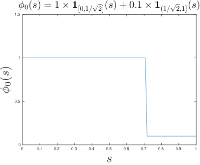
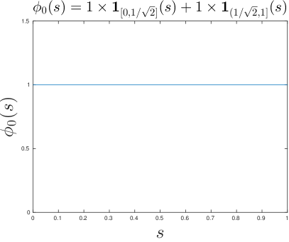
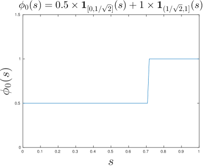
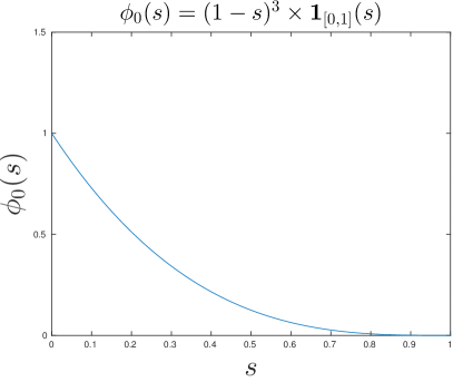
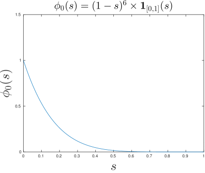
Figure 1: The plots of the influence functions $\phi_{0}(s)$.

We compute the key quantity $q_{\mathrm{max}}$ by exploring all possible $q$ in $[0,100]$:

$$q_{\max}=\underset{R_{0}q\in\mathcal{K},0<q\leq 100}{\arg\max}\left[2q\int_{0}^{1}\phi_{0}(s)s\sin(qs)ds\right].$$

We find that for the cases of $\phi_{0}^{3}$ and $\phi_{0}^{4}$, $q_{\max}$ are not unique and the non-uniqueness of $q_{\max}$ will greatly affect the results of the consensus convergence. The parameters we use for the simulation are $\Delta t=0.1$, $L=10$, $R_{0}=1$ and $N=500$. For each $\phi_{0}$, we also plot the function $\psi(s)=2q\int_{0}^{1}\phi_{0}(s)s\sin(qs)ds$; the stars in the plots are the values of $\psi(s)$ at $R_{0}q\in\mathcal{K}$ and the lines are the continuum approximation.

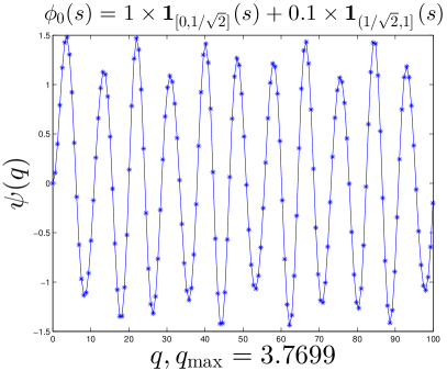
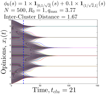
Figure 2: Simulation for $\phi_{0}(s)=\phi^{1}_{0}(s)$. Left: $\psi(q)$ evaluated at $R_{0}q\in\mathcal{K}$. Right: Simulations of (17). The vertical dashed line is at $t=t_{clu}$.

From Figure 2, we can see that there is a unique $q_{\mathrm{max}}=3.7699$. From our analysis, we do not expect to have consensus convergence because $q_{\mathrm{max}}=3.7699<2\pi$. The distance between clusters is $2\pi R_{0}/q_{\mathrm{max}}=1.67$, and therefore we should have roughly $L/1.67=5.99$ clusters, and indeed we have 6 clusters in our simulation. In addition, $t_{clu}=\ln N/(2\rho_{0}R_{0}\psi(q_{\mathrm{max}}))=21$ (the vertical blue dashed line) also correctly predicts the time to cluster formation.

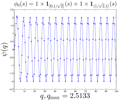
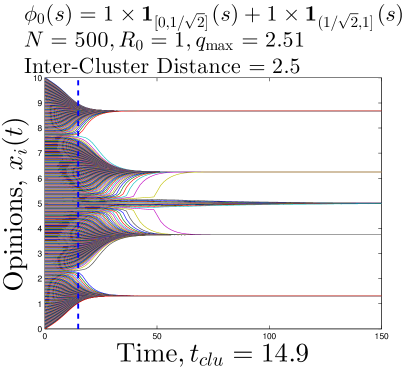
Figure 3: Simulation for $\phi_{0}(s)=\phi^{2}_{0}(s)$. Left: $\psi(q)$ evaluated at $R_{0}q\in\mathcal{K}$. Right: Simulations of (17). The vertical dashed line is at $t=t_{clu}$.

In Figure 3, if $\phi_{0}(s)=\mathbf{1}_{[0,1]}(s)$, then $\psi(q)$ has a unique $q_{\mathrm{max}}=2.51$ but it also has many suboptimal $q$ where $\psi(q)$ is very close to $\psi(q_{\mathrm{max}})$. Note that $q_{\mathrm{max}}<2\pi$ means that there is no consensus convergence. The inter-cluster distance is $2.5$, which is correct for the top and the bottom clusters. However, the central clusters are affected by the suboptimal $q$ and therefore their inter-cluster distances are different. We also note that $t_{clu}=\ln N/(2\rho_{0}R_{0}\psi(q_{\mathrm{max}}))=14.9$ (the vertical blue dashed line) correctly estimates the time to the formation of the top and bottom clusters.

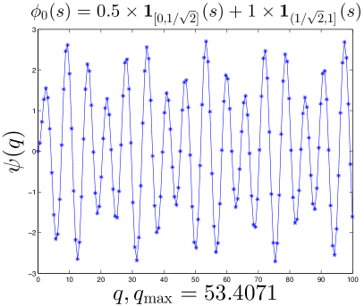
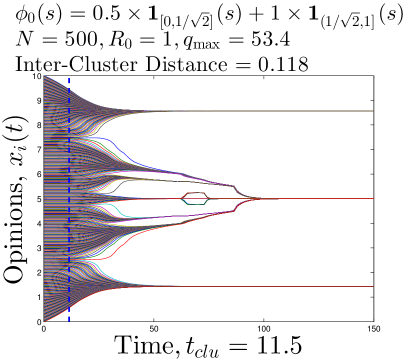
Figure 4: Simulation for $\phi_{0}(s)=\phi^{3}_{0}(s)$. Left: $\psi(q)$ evaluated at $R_{0}q\in\mathcal{K}$. Right: Simulations of (17). The vertical dashed line is at $t=t_{clu}$.

We see an interesting result in Figure 4 for $\phi_{0}(s)=0.5\times\mathbf{1}_{[0,1/\sqrt{2}]}(s)+\mathbf{1}_{(1/\sqrt{2},1]}(s)$. From the plot of $\psi(q)$, we can see that $q_{\mathrm{max}}$ might not be unique and the first few local maximizers are $q=2.5133$, $9.4248$, $15.7080,\ldots$, and the corresponding inter-cluster distances are $2.5$, $0.6667$, $0.4000,\ldots$. We can see from the simulation that there are two noticeable inter-cluster distances: $2.5$ and $0.6667$. For $R_{0}q\in\mathcal{K}$, $0\leq q\leq 100$, $q_{\mathrm{max}}=53.4071$ so that the necessary condition to have the consensus convergence $q_{\mathrm{max}}>2\pi$ is satisfied. However, we do not have consensus convergence in this case because $q_{\mathrm{max}}>2\pi$ is not a sufficient condition. We notice that although $q_{\mathrm{max}}$ might not be unique, $t_{clu}=11.5$ still predicts the time to cluster formation because it is related to $\psi(q_{\mathrm{max}})$ not $q_{\mathrm{max}}$ and thus the non-uniqueness of $q_{\mathrm{max}}$ does not affect $t_{clu}$.

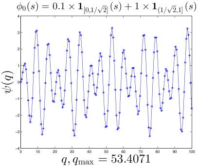
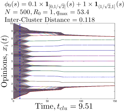
Figure 5: Simulation for $\phi_{0}(s)=\phi^{4}_{0}(s)$. Left: $\psi(q)$ evaluated at $R_{0}q\in\mathcal{K}$. Right: Simulations of (17) for $t\leq 150$. The vertical dashed line is at $t=t_{clu}$.

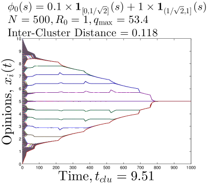
Figure 6: Simulation for $\phi_{0}(s)=\phi^{4}_{0}(s)$. Simulations of (17) for $t\leq 1000$.

In Figure 5 and 6, we see consensus convergence. From the plot of $\psi(q)$, we can see that $q_{\max}$ might not be unique and the first few local maximizers are $q=2.5133$, $9.4248$, $16.3363,\ldots$, and the corresponding inter-cluster distances are $2.5$, $0.6667$, $0.3846,\ldots$. In this case, the only noticeable inter-cluster distance is $0.6667$ and we do not observe the inter-cluster distance of $2.5$, because $\psi(2.5133)\ll\psi(9.4248)$. For $R_{0}q\in\mathcal{K}$, $0\leq q\leq 100$, $q_{\max}=53.4071$ so that the necessary condition to have the consensus convergence $q_{\max}>2\pi$ is satisfied and indeed we see form Figure 6 that we have consensus convergence in this case.

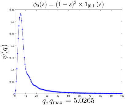
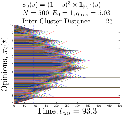
Figure 7: Simulation for $\phi_{0}(s)=\phi^{5}_{0}(s)$. Left: $\psi(q)$ evaluated at $R_{0}q\in\mathcal{K}$. Right: Simulations of (17). The vertical dashed line is at $t=t_{clu}$.

In Figure 7, we choose $\phi_{0}(s)$ so that $\psi(s)$ has a unique local maximum and $q_{\max}=5.0265$. In this case, $q_{\max}<2\pi$ and therefore there is no consensus convergence. The inter-distance is $1.25$ and $L/1.25=8$ which is exactly the number of clusters in this case. Again, $t_{clu}$ predicts the time to cluster formation very well.

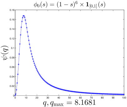
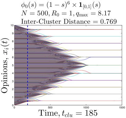
Figure 8: Simulation for $\phi_{0}(s)=\phi^{6}_{0}(s)$. Left: $\psi(q)$ evaluated at $R_{0}q\in\mathcal{K}$. Right: Simulations of (17). The vertical dashed line is at $t=t_{clu}$.

Finally, Figure 8 considers $\phi_{0}(s)$ so that $\psi(s)$ has a unique local maximum, but with a larger exponent, $q_{\max}=8.1681>2\pi$. The inter-cluster distance corresponding to $q_{\max}=8.1681$ is $0.769$, which is consistent with the actual inter-cluster distance. The quantity $L/0.769=13$ gives a good approximation for the actual number of clusters, which is $11$. As in all the previous cases, $t_{clu}=185$ predicts the time to cluster formation well. Here, $q_{\max}>2\pi$, so we could expect to observe consensus convergence. However the inter-cluster distance $0.769$ is such that $\phi(0.769)\sim 10^{-4}$, so we cannot see cluster evolution for the time horizon of the simulation.

5 Stochastic consensus convergence: $\sigma>0$

In this section, we consider the case that $\sigma>0$ in (1). In other words, the system is stochastic and we are dealing with a nonlinear Fokker-Planck equation.

5.1 Linear stability analysis

As in the deterministic case, we linearize the Fokker-Planck equation (5) with $\sigma>0$ by assuming that $\rho(t,x)=\rho_{0}+\rho_{1}(t,x)=1/L+\rho_{1}(t,x)$. Substituting $\rho(t,x)=\rho_{0}+\rho_{1}(t,x)$ into (5) and assuming that $\rho_{1}$ is a small perturbation of $\rho$ so that the $O(\rho_{1}^{2})$ term is negligible, we find that $\rho_{1}(t,x)$ satisfies:

$$\frac{\partial\rho_{1}}{\partial t}(t,x)=\rho_{0}\int\frac{\partial\rho_{1}}{\partial x}(t,x-y)y\phi(|y|)dy+\frac{\sigma^{2}}{2}\frac{\partial^{2}\rho_{1}}{\partial x^{2}}(t,x).$$ (18)

In the Fourier domain:

$$\frac{\partial\hat{\rho}_{1}}{\partial t}(t,k)=\left[i\rho_{0}k\int e^{-iky}y\phi(|y|)dy-\frac{\sigma^{2}k^{2}}{2}\right] \hat{\rho}_{1}(t,k),$$ (19)

which gives the growth rates of the modes:

$$\gamma_{k}=\mathrm{Re}\left[i\rho_{0}k\int e^{-iky}y\phi(|y|)dy-\frac{\sigma^{2}k^{2}}{2}\right]=\rho_{0}k\int\sin(ky)y\phi(|y|)dy-\frac{\sigma^{2}k^{2}}{2}.$$ (20)

We can rewrite the growth rate $\gamma_{k}=\rho_{0}R_{0}\psi_{\sigma}(kR_{0})$, where

$$\psi_{\sigma}(q)=2q\int_{0}^{1}\phi_{0}(s)s\sin(qs)ds-\frac{\sigma^{2}q^{2}}{2\rho_{0}R_{0}^{3}}.$$ (21)

The optimal positive frequency is $k_{\max}$ that is the element of $\mathcal{K}=\{2\pi n/L,n\in\mathbb{N}\}$ that maximizes $\psi_{\sigma}(kR_{0})$, that is close to $q_{\max}/R_{0}$, where

$$q_{\max}=\underset{q>0}{\arg\max}\left[\psi_{\sigma}(q)\right].$$ (22)

There is a critical value $\sigma_{c}$ of $\sigma$ such that the system has a completely different overall behavior for $\sigma<\sigma_{c}$ and for $\sigma>\sigma_{c}$. We can view $\sigma$ as the magnitude of the noise energy or temperature of the system. There are two types of forces in the system (1): the attractive interaction $-a_{ij}(x_{i}-x_{j})$ and the random force $\sigma dW^{i}(t)$. If $\sigma<\sigma_{c}$, then the attractive interaction dominates the random force and thus the system is a perturbation of the deterministic system. If $\sigma>\sigma_{c}$, then the random force dominates, the attractive interaction is negligible, and therefore the overall system behaves like a system of $N$ independent random processes.

The above observations can be articulated mathematically. Let

$$\sigma_{c}^{2} =\max_{q>0}\left[\frac{4\rho_{0}R_{0}^{3}}{q}\int_{0}^{1}\phi_{0}(s)s\sin(qs)ds\right]$$

$$=\max_{q>0}\left[4\rho_{0}R_{0}^{3}\int_{0}^{1}\phi_{0}(s)s^{2}\frac{\sin(qs)}{qs}ds\right]=4\rho_{0}R_{0}^{3}\int_{0}^{1}s^{2}\phi_{0}(s)ds.$$

If $\sigma<\sigma_{c}$, then from (21) we find that

$$\max_{q>0}\psi_{\sigma}(q)>0,$$ (23)

and $\hat{\rho}(t,k_{\max})$ has positive growth rate $\gamma_{\max}=\rho_{0}R_{0}\psi_{\sigma}(k_{\max}R_{0})$. The linear system (19) is unstable, which is analogous to the deterministic case.

If $\sigma>\sigma_{c}$, then all of $\hat{\rho}(t,k)$ have negative growth rates. In other words, the constant density is linearly stable and therefore the overall system is stable, since this is what linear stability implies in this case.

We note that the same technique for computing $\sigma_{c}$, with linear stability analysis for different noisy opinion models, is also used in Pineda2009 Pineda2011 Pineda2013 .

5.2 Fluctuation theory

Since our goal is to analyze the behavior of clusters, we suppose from now on that $\sigma<\sigma_{c}$.

The fluctuation analysis of the stochastic model is similar to that of the deterministic case. If $x_{1}(0),\ldots,x_{N}(0)$ are independent, uniform random variables in $[0,L]$, then

$$\rho^{N}_{1}(t=0,dx):=\sqrt{N}\left(\rho^{N}(t=0,dx)-\rho_{0}(dx)\right)=\sqrt{N}\left(\frac{1}{N}\sum_{j=1}^{N}\delta_{x_{j}(0)}(dx)-\frac{dx}{L}\right)$$

converges in distribution as $N\to\infty$ to the measure $\rho_{1}(t=0,dx)$, whose frequency components

$$\hat{\rho}_{1}(t=0,k)=\lim_{N\to\infty}\sqrt{N}\left(\frac{1}{N}\sum_{j=1}^{N}e^{-ikx_{j}(0)}\right)$$

are independent complex circular Gaussian random variables, with mean zero and variance $1$ for $k\in{\cal K}\backslash\{0\}$:

$$\mathbb{E}\left[\hat{\rho}_{1}(t=0,k)\right]=0,\quad\mathbb{E}\left[\hat{\rho}_{1}(t=0,k)\overline{\hat{\rho}_{1}(t=0,k^{\prime})}\right]=\delta_{kk^{\prime}},\quad k,k^{\prime}\in{\cal K}\backslash\{0\},$$

$\hat{\rho}_{1}(t=0,-k)=\overline{\hat{\rho}_{1}(t=0,k)}$, while $\hat{\rho}_{1}(t=0,k=0)=0$.

For any $T<\infty$, the measure-valued process

$$\rho^{N}_{1}(t,dx):=\sqrt{N}\left(\rho^{N}(t,dx)-\rho_{0}(dx)\right),\quad t\in[0,T]$$ (24)

converges in distribution as $N\to\infty$ to a measure-valued process $\rho_{1}(t,dx)$ whose density $\rho_{1}(t,x)$ satisfies a stochastic PDE (see Dawson1983 ):

$$d\rho_{1}(t,x)=\left[\rho_{0}\int\frac{\partial\rho_{1}}{\partial x}(t,x-y)y\phi(|y|)dy+\frac{\sigma^{2}}{2}\frac{\partial^{2}\rho_{1}}{\partial x^{2}}(t,x)\right]dt+\sigma dW(t,x)$$ (25)

with the random initial condition described above. Here $W(t,x)$ is a space-time Gaussian random noise with mean zero and covariance

$${\rm Cov}\left(\int_{0}^{L}W(s,x)f_{1}(x)dx,\overline{\int_{0}^{L}W(t,x)f_{2}(x)dx}\right)=\frac{\min\{s,t\}}{L}\int_{0}^{L}f^{\prime}_{1}(x)\overline{f^{\prime}_{2}(x)}dx$$ (26)

for any test functions $f_{1}(x)$ and $f_{2}(x)$. The Fourier transform of $W(t,x)$ is $\hat{W}(t,k)=\int_{0}^{L}W(t,x)e^{-ikx}dx$ for $k\in{\cal K}$. From (26), we see that $\{\hat{W}(t,k),k\in{\cal K},k\geq 0\}$ are independent, complex-valued Brownian motions with the variance:

$${\rm Cov}\left(\hat{W}(t,k),\overline{\hat{W}(t,k)}\right)=\frac{t}{L}\int_{0}^{L}(-ik)e^{-ikx}\overline{(-ik)e^{-ikx}}dx=tk^{2},$$ (27)

and $\hat{W}(t,-k)=\overline{\hat{W}(t,k)}$. Taking the Fourier transform on (25), for each $k\in{\cal K}$, $\hat{\rho}_{1}(t,k)=\int_{0}^{L}\rho_{1}(t,x)e^{-ikx}dx$ is a complex-valued Ornstein-Uhlenbeck (OU) process:

$$d\hat{\rho}_{1}(t,k)=\left[i\rho_{0}k\int_{0}^{L}e^{-iky}y\phi(|y|)dy-\frac{\sigma^{2}k^{2}}{2}\right]\hat{\rho}_{1}(t,k)dt+\frac{\sigma k}{\sqrt{2}}d(W^{(k)}(t)+i\tilde{W}^{(k)}(t)).$$ (28)

Here $\{W^{(k)}(t),k\in{\cal K},k>0\}$ and $\{\tilde{W}^{(k)}(t),k\in{\cal K},k>0\}$ are independent real Brownian motions, $W^{(0)}(t)=\tilde{W}^{(0)}(t)=0$, ${W}^{(-k)}(t)=-{W}^{(k)}(t)$, and $\tilde{W}^{(-k)}(t)=\tilde{W}^{(k)}(t)$. The equation (28) is solvable and we have, for any $k\in{\cal K}\backslash\{0\}$,

$$\hat{\rho}_{1}(t,k) =e^{\alpha_{k}t}\hat{\rho}_{1}(0,k)+\frac{\sigma k}{\sqrt{2}}\int_{0}^{t}e^{\alpha_{k}(t-s)}d(W^{(k)}(s)+i\tilde{W}^{(k)}(s)),$$ (29)

$$\alpha_{k} =i\rho_{0}k\int_{0}^{L}e^{-iky}y\phi(|y|)dy-\frac{\sigma^{2}k^{2}}{2}.$$

In particular, $\hat{\rho}_{1}(t,k=0)=0$. Because $\{\hat{\rho}_{1}(0,k),W^{(k)}(t),\tilde{W}^{(k)}(t),k\in{\cal K},k>0\}$ are independent, $\{\hat{\rho}_{1}(t,k),k\in{\cal K},k>0\}$ are independent OU processes with mean zero and variance

$$\mathbb{E}\left[\hat{\rho}_{1}(t,k)\overline{\hat{\rho}_{1}(t,k)}\right]=e^{2\gamma_{k}t}+\sigma^{2}k^{2}\int_{0}^{t}e^{2\gamma_{k}(t-s)}ds=e^{2\gamma_{k}t}\left[1+\frac{\sigma^{2}k^{2}}{2\gamma_{k}}\right],$$ (30)

for $k\in{\cal K}$, $k>0$, where $\gamma_{k}$ is the real part of $\alpha_{k}$. In addition, because $\alpha_{-k}=\overline{\alpha_{k}}$ and $W^{(-k)}(t)=-W^{(k)}(t)$, we have $\hat{\rho}_{1}(t,-k)=\overline{\hat{\rho}_{1}(t,k)}$ for $k\in{\cal K}\backslash\{0\}$. Finally, $\hat{\rho}_{1}(t,0)=0$. Therefore,

$$\mathbb{E}\left[\rho_{1}(t,x)\rho_{1}(t,x^{\prime})\right]=\mathbb{E}\left[\sum_{k}\hat{\rho}_{1}(t,k)\frac{e^{ikx}}{L}\sum_{k}\hat{\rho}_{1}(t,k)\frac{e^{ikx^{\prime}}}{L}\right]$$

$$\quad=\sum_{k}\mathbb{E}\left[\hat{\rho}_{1}(t,k)\frac{e^{ikx}}{L}\hat{\rho}_{1}(t,-k)\frac{e^{-ikx^{\prime}}}{L}\right]=\frac{1}{L^{2}}\sum_{k\neq 0}e^{2\gamma_{k}t}e^{ik(x-x^{\prime})}\left[1+\frac{\sigma^{2}k^{2}}{2\gamma_{k}}\right].$$

As $t$ increases, the spectrum of $\rho_{1}(t,x)$ becomes concentrated around the optimal wavenumber $k_{\max}$. In addition, we note that $k^{2}/\gamma_{k}$ is bounded and the term $\sigma^{2}k^{2}/\gamma_{k}$ is negligible if $\sigma$ is sufficiently small. We can assume $\sigma$ is small because we need $\sigma<\sigma_{c}$ for cluster formation. If $\sigma^{2}k^{2}/\gamma_{k}$ is negligible and $L^{2}\gg 4|\gamma_{\max}^{\prime\prime}|t$, we can expand $\gamma_{k}=\gamma_{\max}+\frac{1}{2}\gamma_{\max}^{\prime\prime}(k-k_{\max})^{2}$ for $k$ around $k_{\max}$, and use a continuum approximation for the discrete sum as we do in the deterministic case:

$$\mathbb{E}\left[\rho_{1}(t,x)\rho_{1}(t,x^{\prime})\right]\simeq\left(\frac{1}{L}e^{2\gamma_{\max}t}\cos(k_{\max}(x-x^{\prime}))\right)\left(\frac{1}{\sqrt{\pi|\gamma_{\max}^{\prime\prime}|t}}e^{-\frac{(x-x^{\prime})^{2}}{4|\gamma_{\max}^{\prime\prime}|t}}\right).$$

If $L^{2}\ll 4|\gamma_{\max}^{\prime\prime}|t$, then the continuum approximation is not valid and in this case

$$\mathbb{E}\left[\rho_{1}(t,x)\rho_{1}(t,x^{\prime})\right]\simeq\frac{2}{L^{2}}e^{2\gamma_{\max}t}\cos\left(k_{\max}(x-x^{\prime})\right)\left[1+\frac{\sigma^{2}k_{\max}^{2}}{2\gamma_{\max}}\right].$$

Because $\sigma<\sigma_{c}$ we have that $\gamma_{\max}>0$ and then the linear system (25) is unstable and therefore the central limit theorem breaks down when $\rho_{1}(t,x)/\sqrt{N}$ is no longer smaller than $\rho_{0}=1/L$. More precisely, the time $t_{clu}$ for the onset of clustering is when $\mathbb{E}\big{[}\rho_{1}(t_{\rm clu},x)^{2}\big{]}\simeq NL^{-2}$, which is approximately

$$t_{clu}\simeq\frac{1}{2\gamma_{\max}}\ln N\simeq\frac{1}{2\rho_{0}R_{0}\psi_{\sigma}(q_{\max})}\ln N$$

when $N\gg 1$.

5.3 Consensus convergence

We assume $\sigma<\sigma_{c}$ so that there are unstable modes for the linearized evolution, which means that there is clustering. The number of and the distance between clusters can be estimated with $q_{\max}$. We find that the first term of the right side of (21) is bounded while the second term of (21) is quadratic with negative leading coefficient. Therefore, increasing $\sigma$ tends to reduce $q_{\max}$, that is to say, to increase the mean distance between clusters.

Let us consider the case that $q_{\max}<2\pi$. From the analysis of the deterministic case, the system initially has no consensus convergence and there are several clusters. After clustering, the clusters do not interact with each other, but their centers move like independent Brownian motions. When two clusters come close to each other, within a distance $R_{0}$, they interact and merge. Therefore, we will eventually have consensus convergence, because two Brownian motions always collide in $\mathbb{R}$. This can be extended to the multi-dimensional case, but then the conclusion can be different: in high dimension two Brownian motions may not collide. However, with periodic boundary conditions, two Brownian motions will always come close to each other, within a distance $R_{0}$.

When $q_{\max}<2\pi$ and $\sigma$ is small then there are several clusters, after the cluster formation time. The fraction of agents in a cluster is the agent density times the inter-distance of the clusters:

$$m_{c}=\rho_{0}\frac{2\pi R_{0}}{q_{\max}}=\rho_{0}\frac{2\pi}{k_{\max}}.$$

Then the $j$-th cluster consists of about $Nm_{c}$ agents. We assume that $\sigma$ is small enough so that $\sigma^{2}k_{\max}\ll 2\pi\rho_{0}\phi_{0}(0)R_{0}^{2}$. By using the fact that the agents in a cluster stay close to each other, we can replace $\phi(x_{i}-x_{j})$ by $\phi(0)$, and the agents in the $j$-th cluster have the approximate dynamics:

$$dx^{(j)}_{i}=-\frac{\phi_{0}(0)}{N}\sum_{l=1}^{Nm_{c}}(x^{(j)}_{i}-x^{(j)}_{l})dt+\sigma dW^{(j,i)}(t).$$

The center $X^{(j)}(t)=\frac{1}{Nm_{c}}\sum_{i=1}^{Nm_{c}}x^{(j)}_{i}(t)$ satisfies:

$$X^{(j)}(t)=X^{(j)}(0)+\frac{\sigma}{\sqrt{Nm_{c}}}W^{(j)}(t),$$ (31)

where $\{W^{(j)}(t)\}$ are independent standard Brownian motions.

When $N$ is large, the empirical density $\frac{1}{Nm_{c}}\sum_{i=1}^{Nm_{c}}\delta_{x^{(j)}_{i}}(dx)$ is approximately a Gaussian density

$$\rho^{(j)}(t,dx)=\frac{1}{\sqrt{\pi(\sigma^{(j)})^{2}}}\exp\left(-\frac{(x-X^{(j)}(t))^{2}}{(\sigma^{(j)})^{2}}\right)dx,\quad\sigma^{(j)}=\frac{\sigma}{\sqrt{m_{c}\phi_{0}(0)}}.$$ (32)

For this argument to be valid, we must have that $\sigma^{(j)}$, the width of $\rho^{(j)}$, is much smaller than $R_{0}$, which is equivalent to our assumption $\sigma^{2}k_{\max}\ll 2\pi\rho_{0}\phi_{0}(0)R_{0}^{2}$.

This cluster dynamics is valid as long as the centers $\{X^{(j)}(t)\}$ stay away from each other by a distance larger than $R_{0}$. The clusters move, according to independent Brownian motions with quadratic variation $\frac{\sigma^{2}t}{Nm_{c}}$. When two clusters come close to each other within a distance $R_{0}$, they merge. Indeed, once the two centers are within distance $R_{0}$, they obey the following differential equations to leading order in $N$:

$$\frac{dX^{(k)}(t)}{dt} =-m_{c}(X^{(k)}(t)-X^{(l)}(t))\phi(X^{(k)}(t)-X^{(l)}(t)),$$

$$\frac{dX^{(l)}(t)}{dt} =-m_{c}(X^{(l)}(t)-X^{(k)}(t))\phi(X^{(k)}(t)-X^{(l)}(t)),$$

which shows that the inter-cluster distance converges exponentially fast to zero and the center converges to the average of the centers just before collision. The number of agents or mass of the new cluster is the sum of the masses of the two clusters, the inverse square width of its empirical density is the sum of the inverse squares of the two widths, its center is at the weighted average (weighted by the masses) of the two centers just before collision and it moves as a Brownian motion whose diffusion constant is defined in terms of its new mass. Then the cluster centers move according to Brownian motions until two of them get within the distance $R_{0}$ from each other and a new merge event occurs. This eventually forms a Markovian dynamics described in the next section.

5.4 Markovian dynamics of the clusters

After the initial clusters are formed, we can use an iterative argument to mathematically describe how all the opinions converge eventually. In the initial configuration, at time $\tau_{0}$, there are $M(\tau_{0})=Lk_{\max}/2\pi$ clusters with centers $X^{(j)}(\tau_{0})=j2\pi/k_{\max}$ (up to a global shift), widths $\sigma^{(j)}(\tau_{0})=\sigma/\sqrt{m_{c}\phi_{0}(0)}$, and masses $m^{(j)}(\tau_{0})=m_{c}$ for $j=1,\ldots,M(\tau_{0})$.

For $t\geq\tau_{n-1}$, there are $M(\tau_{n-1})$ clusters moving as

$$X^{(j)}(t)=X^{(j)}(\tau_{n-1})+\sigma^{(j)}(\tau_{n-1})\frac{\sqrt{\phi_{0}(0)}}{\sqrt{N}}\left(W^{(j)}(t)-W^{(j)}(\tau_{n-1})\right)$$

until the stopping time

$$\tau_{n}=\inf\left\{t>\tau_{n-1}:|X^{(k)}(t)-X^{(l)}(t)|=R_{0},\mbox{ for some }k\neq l\right\}.$$

Then the two colliding clusters (with indices $k$ and $l$) merge with the new center

$$\tilde{X}(\tau_{n}^{+})=\frac{m^{(k)}(\tau_{n-1})X^{(k)}(\tau_{n}^{-})+m^{(l)}(\tau_{n-1})X^{(l)}(\tau_{n}^{-})}{m^{(k)}(\tau_{n-1})+m^{(l)}(\tau_{n-1})},$$

the new mass

$$\tilde{m}(\tau_{n})=m^{(k)}(\tau_{n-1})+m^{(l)}(\tau_{n-1})$$

and the new width

$$\tilde{\sigma}(\tau_{n})=\frac{\sigma}{\sqrt{\tilde{m}(\tau_{n})\phi_{0}(0)}}$$

The clusters are relabeled to take into account this merging so that there are $M(\tau_{n})=M(\tau_{n-1})-1$ clusters. The above process is repeated until $n=(Lk_{\max}/2\pi)-1$, when we have only one cluster, and hence consensus convergence.

Note that the time scale at which collisions and merges occur is of the order of $N$, as the Brownian motions are scaled by $1/\sqrt{N}$.

5.5 Numerical simulations

We use the explicit Euler scheme to simulate the stochastic opinion dynamics (1) when $\sigma>0$:

$$x_{i}^{n+1}=x_{i}^{n}-\frac{1}{N}\sum_{j=1}^{N}\phi(|x_{i}^{n}-x_{j}^{n}|)(x_{i}^{n}-x_{j}^{n})\Delta t+\sigma\Delta W^{n+1}_{i},\quad\phi(s)=\phi_{0}(s/R_{0}),$$ (33)

where $\{W^{n+1}_{i}\}$ are independent Gaussian random variables with mean zero and variance $\Delta t$.

Our analysis is on the torus $[0,L]$, but we simulate (33) on $[0,L]$ with reflecting boundary conditions. As we will see, the simulation results agree with the analysis under periodic assumption. Because here we focus on the effects of the randomness, for simplicity we will work only on the case that $\phi_{0}(s)=\mathbf{1}_{[0,1]}(s)$.

We compute the key quantity $q_{\max}$ by exploring all possible $q$ in $[0,100]$:

$$q_{\max}=\underset{R_{0}q\in\mathcal{K},0<q\leq 100}{\arg\max}\left[2q\int_{0}^{1}\phi_{0}(s)s\sin(qs)ds-\frac{\sigma^{2}q^{2}}{2\rho_{0}R_{0}^{3}}\right].$$

We see form the plots of $\psi_{\sigma}(s)$ that the randomness reduces the possibility of the non-uniqueness of $q_{\max}$ because it adds a negative quadratic term in $\psi_{\sigma}(s)$. With randomness, all of our test cases have a clear, unique $q_{\max}$.

The parameters we use for the simulation are $\Delta t=0.1$, $L=10$, $R_{0}=1$ and $N=500$. For each $\sigma$, we also plot the function $\psi_{\sigma}(s)$ in (21); the stars in the plots are the values of $\psi(s)$ evaluated at $R_{0}q\in\mathcal{K}$ and the lines are the continuum approximation.

We first to test for the effect of $\sigma_{c}$, the critical value for $\sigma$, which makes the system stable or unstable. In our setting, $\sigma_{c}=4\rho_{0}R_{0}^{3}\int_{0}^{1}s^{2}\phi_{0}(s)ds=0.365$ and we simulate (33) for $\sigma=0.1,0.2,0.365,0.5$ that are values below, equal to and above $\sigma_{c}$, respectively.

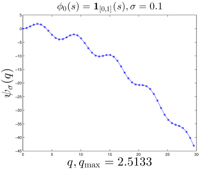
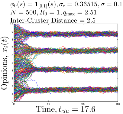
Figure 9: Simulations for $\sigma=0.1$. Left: $\psi_{\sigma}(q)$ evaluated at $R_{0}q\in\mathcal{K}$. Right: Simulations of (33). The vertical dashed line is at $t=t_{clu}$.

From Figure 9, we see that $\psi_{\sigma}(q)$ decreases quadratically and has the unique maximum at $q=2.5133$. However, $\max_{R_{0}q\in\mathcal{K}}\psi_{\sigma}(q)$ is still positive so the linearized system (19) is still unstable. Therefore, the overall system behavior is similar to the deterministic case and can be viewed as a perturbed non-random opinion dynamics.

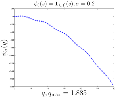
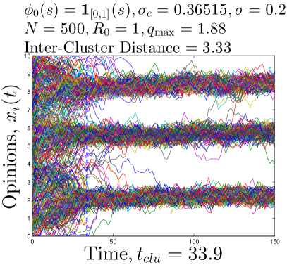
Figure 10: Simulations for $\sigma=0.2$. Left: $\psi_{\sigma}(q)$ evaluated at $R_{0}q\in\mathcal{K}$. Right: Simulations of (33).

We increase $\sigma$ by setting $\sigma=0.2$ and the result is in Figure 10. We see that as $\sigma$ increases, the random noise starts to affect the overall system, and the width and the inter-cluster distances become larger so we observe fewer clusters. Since $\max_{R_{0}q\in\mathcal{K}}\psi_{\sigma}(q)$ is positive, we still observe cluster formation.

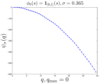
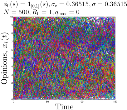
Figure 11: Simulations for $\sigma=\sigma_{c}$. Left: $\psi_{\sigma}(q)$ evaluated at $R_{0}q\in\mathcal{K}$. Right: Simulations of (33).

We note that in Figure 11 and 12, if $\sigma\geq\sigma_{c}$, $\psi_{\sigma}(q)<0$ for all $q>0$ and $\psi_{\sigma}(0)=0$. In other words, the linearized system is stable and thus the full system is stable. In this case, we do not see cluster formation and the system behaves like an $N$-independent agent system.

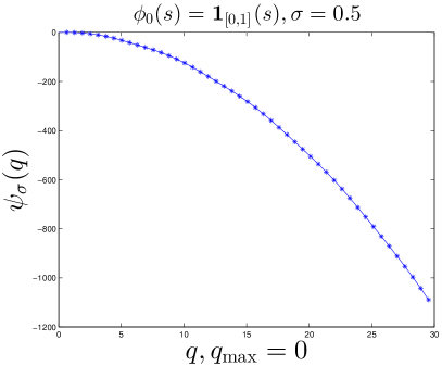
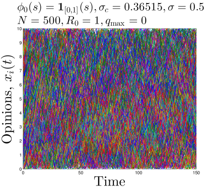
Figure 12: Simulations for $\sigma=0.5$. Left: $\psi_{\sigma}(q)$ evaluated at $R_{0}q\in\mathcal{K}$. Right: Simulations of (33).

We see from the simulations that to model opinion dynamic with consensus convergence it is appropriate to assume that $\sigma<\sigma_{c}$. Therefore we will assume that $\sigma=0.1$ in our simulations of the stochastic system.

We revisit Figure 9 to check our analysis. First of all, $q_{\max}=2.5133$ is clearly a unique maximizer and the corresponding inter-cluster distance is $2.51$, which agrees with the numerical inter-cluster distance we see in Figure 9. In addition, $L/2.51=3.9841$ also predicts well the actual number of the clusters, $4$. Finally, the blue dashed line $t=t_{clu}$ indicates the time to the cluster formation, even though Figure 9 is just one realization.

We test $t_{clu}$ and the width of clusters in a more statistical way by examining $1000$ realizations. If $\phi_{0}(s)=\mathbf{1}_{[0,1]}(s)$ and $\sigma=0.1$, then we can expect that we will have $4$ clusters at $T=150$ in most of the realizations. For each realization, we numerically compute the widths of the clusters, $\hat{\sigma}^{(j)}(t)$, $j=1,\ldots,4$ by using the empirical standard deviations of $\{x^{(j)}_{i}(t)\}_{j=1}^{4}$ (see (32)):

$$(\hat{\sigma}^{(j)}(t))^{2}=\frac{2}{N^{(j)}-1}\sum_{i=1}^{N^{(j)}}\left(x^{(j)}_{i}(t)-\bar{x}^{(j)}(t)\right)^{2},\quad\bar{x}^{(j)}(t)=\frac{1}{N^{(j)}}\sum_{i=1}^{N^{(j)}}x^{(j)}_{i}(t)$$ (34)

where for each $j=1,\ldots,4$, $\{x^{(j)}_{i}(t)\}$ belong to the $j$-th cluster and $N^{(j)}$ is the number of agents in the j-th clusters. Of course, $\hat{\sigma}^{(j)}(t)$ in (34) is just one realization and so we compute $\hat{\sigma}^{(j)}(t)$ for $1000$ realizations and consider the average.

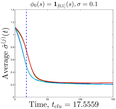
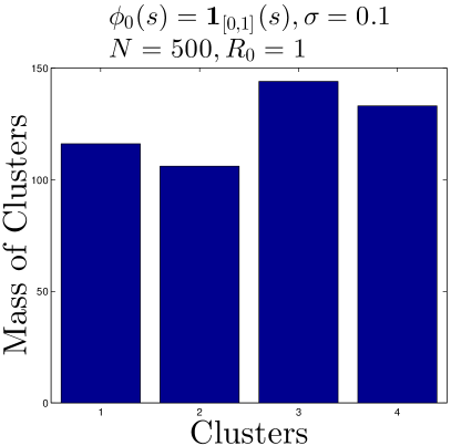
Figure 13: Left: Average of $1000$ realizations of $\hat{\sigma}^{(j)}(t)$, $j=1,\ldots,4$ for $\sigma=0.1$. The vertical dashed line is at $t=t_{clu}$. Right: $N^{(j)}$, the number of agents in the $j$-th clusters in Figure 9.

The averages $\hat{\sigma}^{(j)}(t)$ are shown in the left part of Figure 13, in different colors. First, we can see that $t_{clu}$, as expected, is the halfway from the time to maximum with to the time to the minimum width. Second, from (32), the width of each cluster is analytically $\sigma^{(j)}=\sigma/\sqrt{m_{c}\phi_{0}(0)}=0.1/\sqrt{0.25\times 1}=0.2$, which agrees with the numerical values $\hat{\sigma}^{(j)}(t)$ when $t$ is large.

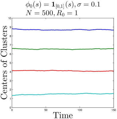
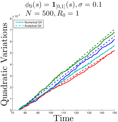
Figure 14: Left: Centers of the clusters, $X^{(j)}(t)$, in Figure 9, in different colors. Right: Quadratic variations of the cluster centers from $t=75$ to $t=150$. Solid lines: Numerical quadratic variations of $X^{(j)}(t)$. Dashed lines: Quadratic variations of $\sigma W^{(j)}(t)/\sqrt{N^{(j)}}$, where $\{W^{(j)}(t)\}_{j=1}^{4}$ are independent standard Brownian motions and $\{N^{(j)}\}_{j=1}^{4}$ are the numbers of agents in the clusters.

We also analyze the behavior of the centers of the clusters. The centers $\{X^{(j)}(t)\}_{j=1}^{4}$ of the clusters in Figure 9 are plotted in Figure 14. From the previous analysis (31), the centers of the clusters are independent Brownian motions $\sigma W^{(j)}(t)/\sqrt{Nm_{c}}$. For one realization, the opinions $\{x_{i}(t)\}_{i=1}^{N}$ will not be evenly distributed in the clusters. For example, the actual numbers $\{N^{(j)}\}_{j=1}^{N}$ of agents of the clusters in Figure 9 are plotted in Figure 13. So for one realization, $X^{(j)}(t)$ is a Brownian motion $\sigma W^{(j)}(t)/\sqrt{N^{(j)}}$. On the right part of Figure 14, we compare the quadratic variations of $X^{(j)}(t)$ and $\sigma W^{(j)}(t)/\sqrt{N^{(j)}}$ for $75\leq t\leq 150$ (after the time to the cluster formation.) Indeed, from the figure, we can see that their quadratic variations are very similar and that means $X^{(j)}(t)$ are very close to Brownian motions.

6 Long time behavior of simulations

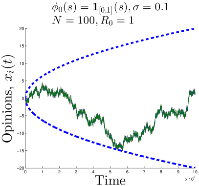
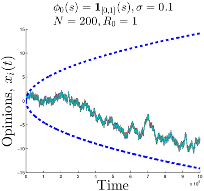
Figure 15: Long time behavior of the opinions for $\sigma=0.1$ and for $N=100,200$. The blue dashed curve is the equation $x=\pm 2\sigma\sqrt{t/N}$. $\sigma$ is small and the overall behavior is like a single Brownian motion.

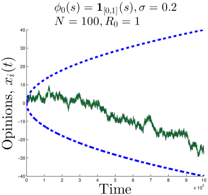
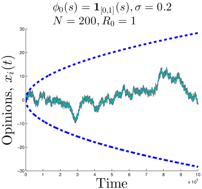
Figure 16: Long time behavior of the opinions for $\sigma=0.2$ and for $N=100,200$. The blue dashed curve is the equation $x=\pm 2\sigma\sqrt{t/N}$. $\sigma$ is small and the overall behavior is like a single Brownian motion.

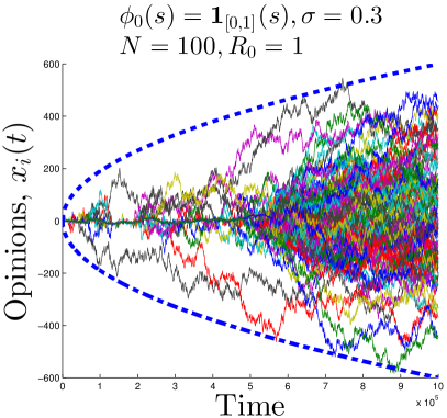
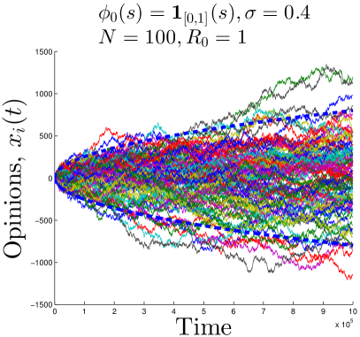
Figure 17: Long time behavior of the opinions for $\sigma=0.3,0.4$ and for $N=100$. The blue dashed curve is the equation $x=\pm 2\sigma\sqrt{t}$. For $\sigma=0.3$, there is a single cluster for $t\leq 5.5\times 10^{5}$. However, for $t>5.5\times 10^{5}$, $x_{i}(t)$ disintegrate and the system behaves like an $N$-independent Brownian motions. For $\sigma=0.4$, the random perturbations are large enough so that the system is an $N$-independent Brownian motions at the beginning.

We have also simulated numerically the long time behavior of the system defined on the full real line $\mathbb{R}$, especially the behavior after the onset of consensus convergence. As we discuss in the previous section, when there is randomness the center of the unique cluster behaves like a diffusion process $\sigma W(t)/\sqrt{N}$, where $W(t)$ is a standard Brownian motion. In Figure 15 and 16, we observe that the centers indeed behave like Brownian motions. The dashed lines are the parabolas with equation $x=\pm 2\sigma\sqrt{t/N}$ so that for any fixed $t$, the centers are within the parabolas with $95\%$ probability.

However, when $\sigma$ is sufficiently large, the long time behavior is different. On the right part of Figure 17, when $\sigma=0.4>\sigma_{c}$, the system behaves like $N$-independent diffusions. A more interesting case is when $\sigma=0.3<\sigma_{c}$ on the left part of Figure 17. In this case, for $0\leq t\leq 5.5\times 10^{5}$ there is still consensus convergence, but for $t>5.5\times 10^{5}$, all $x_{i}(t)$ spread out from the unique cluster and the system becomes an independent agent evolution. A detailed mathematical analysis using large deviations theory for such a phenomenon is being considered at present.

7 Conclusion

We have analyzed a stochastic, continuous time opinion dynamics model and we have carried out extensive numerical simulations. We use the mean-field theory and obtain a nonlinear Fokker-Planck equation as the number of opinions tends to infinity. Then we use a linear stability analysis to estimate the critical value of the noise strength so as to have cluster formation, estimate the number of clusters and the time to cluster formation. These quantities are closely related to the frequency that maximizes the growth rate of the linearized modes (20). After the initial cluster formation we expect, and numerically confirm, that the centers of the clusters behave like Brownian motions before further consolidation. Finally, the long time behavior of the system is explored numerically and we observe that after a unique cluster is formed, there is a small probability that the opinions will spread out from the unique cluster and the system will become an independent agent evolution.

References

- [1] F. Baccelli, A. Chatterjee, and S. Vishwanath. Stochastic bounded confidence opinion dynamics. In Decision and Control (CDC), 2014 IEEE 53rd Annual Conference on, pages 3408–3413, December 2014.
- [2] V.D. Blondel, J.M. Hendrickx, A. Olshevsky, and J.N. Tsitsiklis. Convergence in multiagent coordination, consensus, and flocking. In Decision and Control, 2005 and 2005 European Control Conference. CDC-ECC ’05. 44th IEEE Conference on, pages 2996–3000, December 2005.
- [3] V.D. Blondel, J.M. Hendrickx, and J.N. Tsitsiklis. On the 2R conjecture for multi-agent systems. In Control Conference (ECC), 2007 European, pages 874–881, July 2007.
- [4] C. Canuto, F. Fagnani, and P. Tilli. An Eulerian approach to the analysis of krause’s consensus models. SIAM Journal on Control and Optimization, 50(1):243–265, 2012.
- [5] A. Carro, R. Toral, and M. San Miguel. The Role of Noise and Initial Conditions in the Asymptotic Solution of a Bounded Confidence, Continuous-Opinion Model. Journal of Statistical Physics, 151(1-2):131–149, 2013.
- [6] G. Como and F. Fagnani. Scaling limits for continuous opinion dynamics systems. Ann. Appl. Probab., 21(4):1537–1567, August 2011.
- [7] D. A. Dawson. Critical dynamics and fluctuations for a mean-field model of cooperative behavior. J. Statist. Phys., 31(1):29–85, 1983.
- [8] G. Deffuant, D. Neau, F. Amblard, and G. Weisbuch. Mixing beliefs among interacting agents. Advances in Complex Systems, 03(01n04):87–98, 2000.
- [9] B. Düring, P. Markowich, J.-F Pietschmann, and M.-T. Wolfram. Boltzmann and Fokker–Planck equations modelling opinion formation in the presence of strong leaders. Proceedings of the Royal Society of London A: Mathematical, Physical and Engineering Sciences, 465(2112):3687–3708, 2009.
- [10] J. Gärtner. On the McKean-Vlasov limit for interacting diffusions. Math. Nachr., 137:197–248, 1988.
- [11] J. Gómez-Serrano, C. Graham, and J.-Y. Le Boudec. The bounded confidence model of opinion dynamics. Mathematical Models and Methods in Applied Sciences, 22(02):1150007, 2012.
- [12] S.-Y Ha and E. Tadmor. From particle to kinetic and hydrodynamic descriptions of flocking. Kinetic and Related Methods, pages 415–435, 2008.
- [13] R. Hegselmann and U. Krause. Opinion dynamics and bounded confidence models, analysis, and simulation. Journal of Artificial Societies and Social Simulation, 5(3), 2002.
- [14] R. Hegselmann and U. Krause. Opinion dynamics under the influence of radical groups, charismatic leaders, and other constant signals: A simple unifying model. Networks and Heterogeneous Media, 10(3):477–509, 2015.
- [15] M. Huang and J.H. Manton. Opinion dynamics with noisy information. In Decision and Control (CDC), 2013 IEEE 52nd Annual Conference on, pages 3445–3450, December 2013.
- [16] P.-E. Jabin and S. Motsch. Clustering and asymptotic behavior in opinion formation. Journal of Differential Equations, 257(11):4165–4187, 2014.
- [17] T. G. Kurtz and J. Xiong. Particle representations for a class of nonlinear SPDEs. Stochastic Processes and their Applications, 83(1):103–126, 1999.
- [18] N. Lanchier and J. Neufer. Stochastic dynamics on hypergraphs and the spatial majority rule model. Journal of Statistical Physics, 151(1-2):21–45, 2013.
- [19] J. Lorenz. Continuous opinion dynamics under bounded confidence: a survey. International Journal of Modern Physics C, 18(12):1819–1838, 2007.
- [20] M. Mäs, A. Flache, and D. Helbing. Individualization as driving force of clustering phenomena in humans. PLoS Comput Biol, 6(10):e1000959, 10 2010.
- [21] A. Mirtabatabaei, P. Jia, and F. Bullo. Eulerian Opinion Dynamics with Bounded Confidence and Exogenous Inputs. SIAM Journal on Applied Dynamical Systems, 13(1):425–446, 2014.
- [22] S. Motsch and E. Tadmor. Heterophilious dynamics enhances consensus. SIAM Review, 56(4):577–621, 2014.
- [23] M. Pineda, R. Toral, and E. Hernandez-Garcia. Noisy continuous-opinion dynamics. Journal of Statistical Mechanics: Theory and Experiment, 2009(08):P08001, 2009.
- [24] M. Pineda, R. Toral, and E. Hernandez-Garcia. Diffusing opinions in bounded confidence processes. The European Physical Journal D, 62(1):109–117, 2011.
- [25] M. Pineda, R. Toral, and E. Hernandez-Garcia. The noisy Hegselmann-Krause model for opinion dynamics. The European Physical Journal B, 86(12), 2013.
- [26] Y. Yang, D.V. Dimarogonas, and X. Hu. Opinion consensus of modified hegselmann-krause models. In Decision and Control (CDC), 2012 IEEE 51st Annual Conference on, pages 100–105, December 2012.