A Novel Method for Detecting Extended Sources with VERITAS

Abstract:

The most commonly used techniques for estimating the background contribution in IACT data analysis are the ring background model and the reflected region methods. However, these two techniques are poorly suited for analyses of sources with extensions comparable to the detector’s field of view (greater than $\sim$1^∘). Nearby pulsar wind nebulae, supernova remnants interacting with molecular clouds, and dark matter signatures from galaxy clusters are just a few potentially highly extended source classes. A three dimensional maximum likelihood analysis is in development that seeks to resolve this issue for data from the VERITAS telescopes. The technique incorporates relevant instrument response functions to model the distribution of detected gamma-ray like events in two spatial dimensions. Additionally, we incorporate a third dimension based on a gamma-hadron discriminating parameter. The inclusion of this third dimension significantly improves the sensitivity of the technique to highly extended sources. We present this promising technique as well as systematic studies demonstrating its potential for revealing sources of large extent in VERITAS data.

1 Introduction

Imaging atmospheric Cherenkov telescopes (IACTs) have had great success in detecting sources at TeV energies. However, the sources typically detected are point sources or exhibit only moderate extensions (radial extension $\lesssim$ 0.5^∘). Other instruments with larger fields of view have detected sources with very large extensions ($\gtrsim$1^∘) including the cocoon detected by Fermi-LAT in the Cygnus region, believed to be the result of freshly accelerated cosmic-rays confined within a cavity in the Cygnus X star-forming region [1]. The morphology of the cocoon was characterized using a Gaussian with $\sigma$ = 2.0^∘ $\pm$ 0.2 making it highly extended. Milagro also reported evidence of extended emission (intrinsic full width at half maximum of 2.6^∘${}^{+0.7}_{-0.9}$) [2] coincident with the Fermi-LAT Geminga pulsar [3]. This extended source, identified as MGRO J0632+17, is thus potentially a pulsar wind nebula (PWN). Additionally, dark matter signatures from galaxy clusters can extend over regions larger than a degree [4]. Detecting these sources requires an analysis which can account for all of the emission in the region simultaneously. This is not a trivial task given the analysis techniques used in IACT data analysis. Standard methods for estimating background emission for these instruments are either the ring background model (RBM) or the reflected-region model [5].

The RBM analysis estimates the level of background for a particular region of interest (ON region) by using an annulus, or ring, around the region. In order to obtain an accurate measure of the background the ratio of the ON region to the ring region is typically on the order of $\sim$1/7. The reflected-region model requires observations to be taken offset from the source position. Suitable OFF regions are chosen at positions in the field of view which have similar offsets from the tracking position as the established ON region. For sources with extensions ¿0.5^∘, no OFF regions can be determined and a larger observing offset is needed, reducing sensitivity to the source. Ultimately, the field of view of the instrument limits the size of source which can be observed with this technique. In the RBM highly extended sources may require a larger ON than OFF region, resulting in a poorly determined background. These examples for the RBM and reflected-region analyses of sources with large extensions are predicated on the assumption that the morphology of the source is known. For the most extended sources the morphology is rarely understood with absolute certainty. In this case, determining suitable OFF regions becomes very difficult and a certain amount of self subtraction due to source contamination in the OFF region is almost guaranteed. Thus, a different analysis technique is necessary to detect these sources in VERITAS data.

2 VERITAS

The Very Energetic Radiation Imaging Telescope Array System (VERITAS) is an array of four 12-meter IACTs located at the Fred Lawrence Whipple Observatory (FLWO) in southern Arizona (31^∘40’ N, 110^∘57’ W, 1.3km a.s.l.). The instrument covers an energy range from 85 GeV to ¿ 30 TeV with an energy resolution between 15 - 25%. VERITAS is capable of detecting a point source with 1% the Crab nebula flux in $\sim$25 hours and has an angular resolution (68% containment radius) of ¡0.1^∘ at 1 TeV.

3 VERITAS Maximum Likelihood Method

In order to tackle extended sources in VERITAS data, a three dimensional maximum likelihood method (MLM) is in development. In general, the method of maximum likelihood works by modeling the expected distribution of events in data. A likelihood value L can then be computed from these models according to

$$L(\mathbf{\vec{s}})=\prod\limits_{i=1}^{d}p(\mathbf{\theta}_{\textit{i}}|\mathbf{\vec{s}})$$ (1)

where p is the model, i indexes individual data events, $\theta$ is a set of observables which represent the data, and $\mathbf{\vec{s}}$ is a set of free parameters chosen to maximize L. Typically, the log of the likelihood is computed as this turns the product into a sum and the computation is simplified.

The VERITAS MLM models consist of both a two dimensional spatial model and a mean scaled width model (MSW) for both the $\gamma$-ray (source) and background components. In this way the full log-likelihood for a single observation becomes

$$log(L(\mathbf{\vec{s}}))=N_{obs}log(N_{exp})-N_{exp}+\sum\limits_{i=1}^{d}log\left[S_{src}(\mathbf{\vec{r}}_{\textit{i}}|\mathbf{\vec{s}})\cdot W_{src}(w_{\textit{i}}|\mathbf{\vec{s}})+S_{bkgd}(\mathbf{\vec{r}}_{\textit{i}})\cdot W_{bkgd}(w_{\textit{i}})\right]$$ (2)

To correlate the spatial source model (S_src) with the MSW source model (W_src), the product of the two distributions is taken (similarly for the background component). An additional term is included in the likelihood to model the total expected number of events from both signal and background. The expected number of events in a dataset is taken to be Poisson distributed with expected events N_exp and observed events N_obs. The first two terms in Eq. 2 are based on this assumption. The data is treated as unbinned in the spatial and MSW dimensions and coarsely binned in reconstructed energy. The free parameters are spectral parameters associated with the source being modeled.

It follows that to analyze data from multiple observing positions, each field can be independently modeled and the resulting log-likelihoods summed to get a likelihood for the entire observation set simultaneously. Since all models share the same free parameters (which are independent of the observing conditions between fields) this can be extended to observations which cover a range of observing positions, detector configurations, or even to connect observations from different detectors.

4 Defining the Input Models

In this section, the various models which represent the expected distribution of the data, and how they are derived is detailed. Specific attention will be paid to the source spatial model in Section 4.2 outlining the details of how we incorporate the various instrument response functions (IRFs) from VERITAS. Each model component is derived from either data (primarily for modeling background) or simulated $\gamma$-ray air-showers (for source models). In both cases, events were processed using standard medium cuts for all variables with the exception of MSW in which a larger range was used to better characterize the background models.

4.1 Background Spatial Models

The background spatial models represent the expected distribution of $\gamma$-ray-like events across the field of view. They are derived from observations taken on weak blazars and dwarf spheroidal galaxies. Data taken in the galactic plane is not used to prevent possible contamination from diffuse $\gamma$-rays. These data are first transformed into the spatial coordinate system used in the analysis and then binned into 0.01^∘ spatial bins. A radial acceptance distribution is generated in r² by summing all bins within a range of offsets from the field of view center. This radial acceptance is extrapolated into two dimensions to form the spatial model associated with the expected background.

Because data is used to derive the background spatial models there are two main effects which must be accounted for. The first effect is contamination from any potential source within the field of view which results in an overestimate of the background at the offset of the source. Secondly, stars in the field of view can cause deficits in the surrounding region. To alleviate these effects all bins within a set angular distance of known (or potential) sources and bright stars are excluded. To correct for the excluded regions, each bin of the radial acceptance curve is weighted by the relative number of bins which actually contribute to it.

4.2 Source Spatial Model

In order to produce a $\gamma$-ray source spatial model the formulation from Mattox et al. (1996) Eq. 2 is used [6].

$$S_{src}(\mathbf{\vec{r}}|\mathbf{\vec{s}})=\frac{1}{N}\int_{E_{min}}^{E_{max}}\int_{0}^{\infty}[B(\mathbf{\vec{r}},E^{\prime})\ast P(\mathbf{\vec{r}},E^{\prime})]S(E^{\prime}|\mathbf{\vec{s}})R(\mathbf{\vec{r}},E^{\prime},E)A(\mathbf{\vec{r}},E^{\prime})dE^{\prime}dE$$ (3)

This gives the expected distribution of the source emission as it is observed. B represents the intrinsic source morphology, which in the case of a point source is a delta function centered at the source position. The various instrument response functions (IRFs) accounted for are the point spread function (PSF, P), energy dispersion (R), and effective collection area (A). Additional parameters are the intrinsic source energy spectrum (S), the spatial coordinates in the field of view ($\mathbf{\vec{r}}$), the true $\gamma$-ray energy (E’), and the observed $\gamma$-ray energy (E). To make the computation of this model tractable, certain assumptions are employed. These include finely binning B and P spatially as well as finely binning in E’ . The spatial model then becomes a summation rather than an integration

$$S_{src}(\mathbf{\vec{r}}_{i,j}|\mathbf{\vec{s}})=\sum_{k,m,n}B_{m,n}P_{m,n}(\mathbf{\vec{r}}_{i,j})A_{m,n}(E_{k}^{\prime})\int_{E_{min}}^{E_{max}}R_{m,n}(E,E_{k}^{\prime})dE\int_{E^{\prime}_{k,lower}}^{E^{\prime}_{k,upper}}S(E^{\prime}|\mathbf{\vec{s}})dE^{\prime}.$$ (4)

This now gives the value of the spatial model within a given bin i,j of the spatial map. Potential “smearing” of events due to the instrument resolution is accounted for by summing the contributions from all other bins n,m at position i,j in the spatial map. A pictoral example of the input source model and resulting MLM computed source model for both a point source and 1.5^∘ diameter extended disc source are given in Figures 1 and 2 respectively.

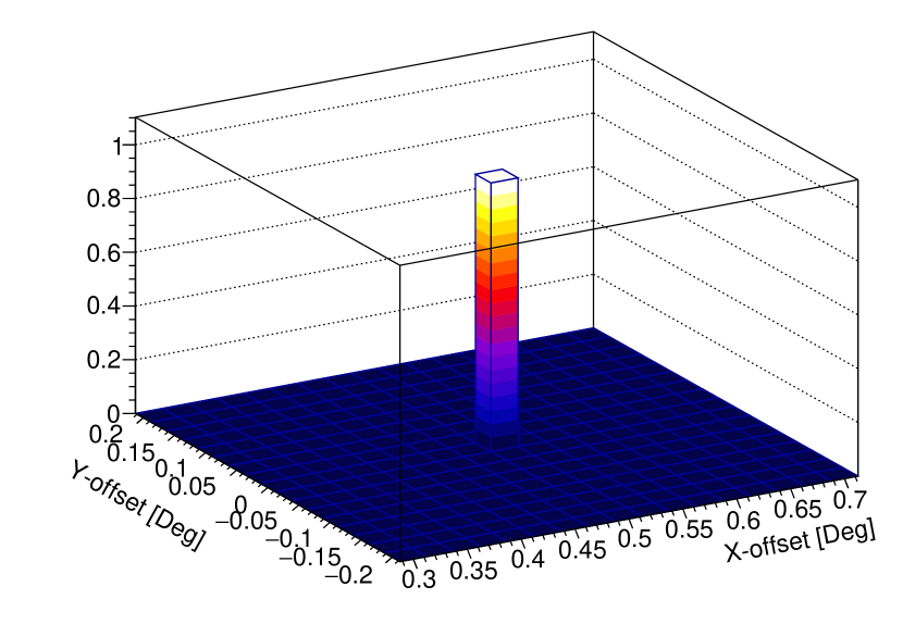
(a) Input point source model

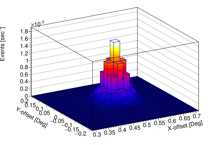
(b) Computed point source model

Figure 1: Example of a computed point source model using Eq. 4. (a) Input source model assuming a delta function at the source position ($\sim$0.5^∘ offset from the camera center). (b) Resulting source model as computed by the MLM described here. For this test case, a Crab-like source spectrum was used.

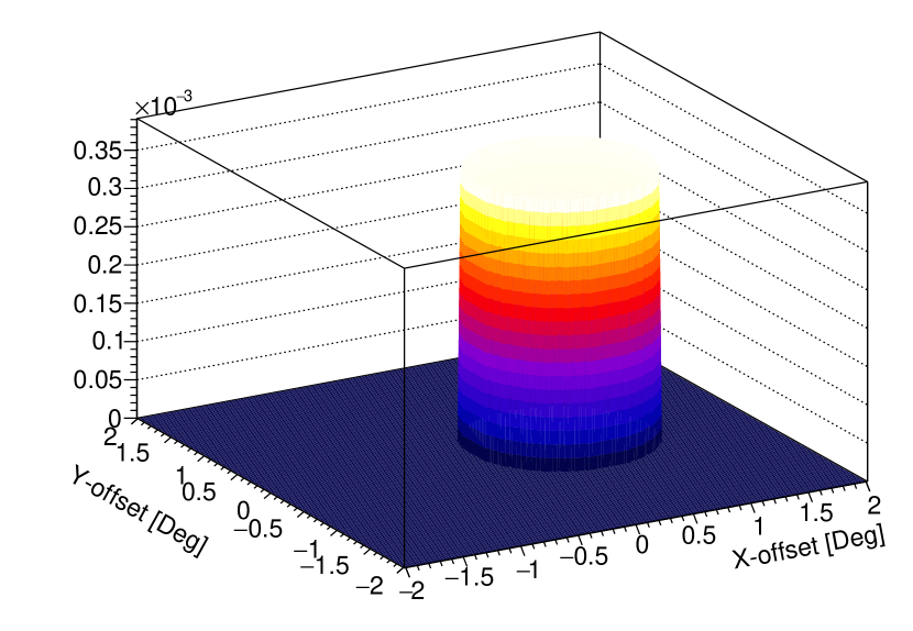
(a) Input extended disc model

(b) Computed extended disc model

Figure 2: Example of a computed extended source model using Eq. 4. (a) Input source model assuming a 1.5^∘ diameter disc centered at 0.5^∘ offset from the camera center. (b) Resulting source model as computed by the MLM. For this test case, a 10% Crab-like source spectrum was used.

This formulation solves an additional challenge. Following Eq. 3 the entire source model and all relavent contributions from each IRF need to be recomputed at each step of the fit. This is computationally intensive. However, using Eq. 4 the component of the source model derived from the IRFs (which are independent of the source spectral parameters) can be precomputed for every bin of E’ requiring only a reweighting of these bins for each iteration of the fit.

The IRFs are parameterized for a range of observing conditions including zenith angle, azimuth, night sky noise level, observing offset from the source, atmospheric conditions, telescope array configuration, and number of telescopes contributing to the shower reconstruction. The PSF is modeled based on fits of a King function to simulated $\gamma$-ray air-shower events generated at fixed energies of 0.1, 0.3, 1, 3, and 10 TeV across the full range of observing conditions listed above.

$$PSF(x,y)\propto\left(1-\frac{1}{\lambda}\right)\left(1+\frac{1}{2\lambda}\cdot\frac{x^{2}+y^{2}}{\sigma^{2}}\right)^{-\lambda}$$ (5)

In particular $\lambda$ and $\sigma$ are computed for each combination of possible observing conditions and interpolated on to obtain a PSF model at any potential observing position and energy. These simulations are also used to generate the energy dispersion of the instrument. As the interpolated energy dispersion becomes less well defined below $\sim$300 GeV (due to limited statistics and the interpolation method used, see Figure 3) the MLM is currently restricted to analysis above this energy.

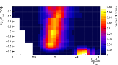
Figure 3: Energy dispersion as a function of logarithmic true energy. The plot represents the fraction of $\gamma$-ray events reconstructed at a given energy (E_rec) as a function of (E_rec-E_true)/E_true. Values are based on fixed-energy $\gamma$-ray air-shower simulations at 70^∘ elevation, 180^∘ azimuth, and offset by 0.25^∘ from the camera center. Simulations are processed using non-standard cuts on MSW and including all events within the field of view. Values are interpolated at energies not represented by the fixed-energy simulations.

4.3 Mean Scaled Width

In order to improve sensitivity to extended sources a third dimension based on a $\gamma$/hadron discriminating parameter known as mean scaled width (MSW) [7] is incorporated. This parameter is based on the average of the Hillas width parameter [8] from images of all participating telescopes normalized by the expected width derived from simulated $\gamma$-ray air-showers.

$$MSW=\left(\frac{1}{n}\right)\sum_{i=1}^{n}\frac{w_{i,j}}{<w_{i}>_{j}}$$ (6)

n is the number of participating telescopes and j represents the various shower parameters over which the expected width value is determined, such as integrated image intensity and impact distance. It follows that $\gamma$-ray events will have a MSW distribution which peaks very close to 1. However, cosmic-rays, which typically result in less compact images, will peak at higher values of MSW (see Figure 4). For the MLM analysis, MSW is restricted to the range 0.8 - 1.3 to provide ample distinction between the source and background models.

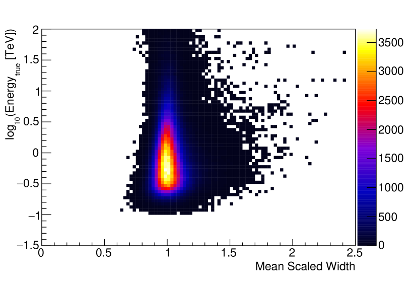
(a) Gamma-ray MSW Distribution

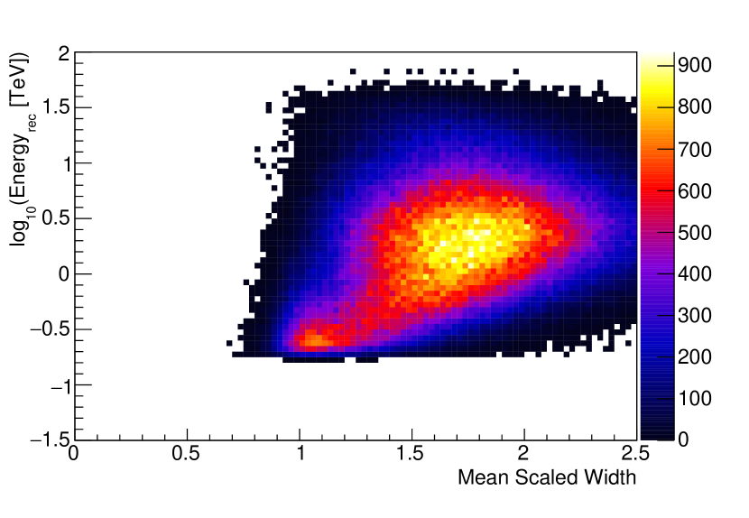
(b) Background MSW Distribution

Figure 4: MSW distributions derived (a) for the source model from simulated $\gamma$-ray air-showers and (b) for the background model from observations. Distributions are shown as a function of logarithmic energy. The color scale represents the number of events used to generate the distribution. Models are extracted for an observation position of 70^∘ elevation, 180^∘ azimuth, and 0.5^∘ offset with four telescopes participating in the shower reconstruction. The slight peak near 1 in the background MSW distribution below $\sim$300 GeV is currently under investigation.

The source MSW model is derived from simulations of $\gamma$-ray air-showers while the background models are derived from actual observations, as mentioned above.

5 Validation Plans

The planned validation of the VERITAS MLM analysis will initially involve a self consistency check in which the generated models are used to produce a sample of toy Monte Carlo events. These generated events will then be fit with the same models to ensure the fitted result is consistent with inputs. The next step will be to fit the models to dedicated OFF observations to check the background models are consistent with data. Once the background models have been verified, a test on the Crab Nebula, a known bright point source, will be conducted to check the source model generation is accurate. Additionally, data has been taken on the Crab Nebula following a raster scan pattern to produce an extended source [9]. Tests on these datasets will provide a check of the extended source fitting using a source with a known spectrum. Finally, the technique will be applied to known extended sources such as supernova remnant G106.3+2.7 [10] and MGRO J1908+06 [11]. Each check is designed to ensure all components of the MLM are understood and behave as expected as well as to identify regions where the technique struggles.

6 Discussion

The expected number of $\gamma$-ray events predicted by the MLM for the Crab-like source model presented in Figure 1 was compared to a sample of observations of the Crab nebula taken under similar observing conditions and analyzed with a standard RBM analysis. The MLM prediction was found to be consistent to within $\sim$10%. Additionally, the extended source (which uses a 10% Crab-like spectrum) actually predicts $\sim$8-9% of the expected Crab flux. This is due to the reduced instrument sensitivity at larger offsets from the center of the field of view which is reflected in the asymmetry of the computed model (see Figure 2(b)).

The analysis is still under development and will undergo a set of optimizations in the future. It will be tested whether extending the range on MSW provides better characterization of the background and thus improved separation between source and background model components. Additionally, how the chosen coarse binning in observed energy affects the result will be investigated. Improvements to the VERITAS shower and energy reconstruction methods will also lead to more accurate IRF parameterizations and thus improve the overall MLM.

Once validated, the technique can be employed on several known extended sources currently undetected by IACTs, such as the cocoon in Cygnus and MGRO J0632+17. This technique also allows the possibility for doing energy-dependent morphology fitting across multiple instruments using a set of common spatial templates. In so doing the VERITAS MLM could be an invaluable tool for multi-wavelength studies in the future.

- [1] M. Ackermann et al., A cocoon of freshly accelerated cosmic rays detected by fermi in the cygnus superbubble, Science 334 (2011), no. 6059 1103–1107.
- [2] A. A. Abdo et al., Milagro Observations of Multi-TeV Emission from Galactic Sources in the Fermi Bright Source List, ApJ Lett. 700 (Aug., 2009) L127–L131, [arXiv:0904.1018].
- [3] A. A. Abdo et al., Fermi-lat observations of the geminga pulsar, ApJ 720 (2010), no. 1 272.
- [4] K. Murase and J. F. Beacom, Galaxy clusters as reservoirs of heavy dark matter and high-energy cosmic rays: constraints from neutrino observations, Jour. Cosmology and Astroparticle Phys. 2013 (2013), no. 02 028.
- [5] D. Berge, S. Funk, and J. Hinton, Background modelling in very-high-energy -ray astronomy, A&A 466 (May, 2007) 1219–1229, [astro-ph/0610959].
- [6] J. R. Mattox et al., The Likelihood Analysis of EGRET Data, ApJ 461 (Apr., 1996) 396.
- [7] M. K. Daniel, The VERITAS standard data analysis, Proceedings of the 30th International Cosmic Ray Conference (2008) 1325–1328, [arXiv:0709.4006].
- [8] A. M. Hillas, Cerenkov light images of EAS produced by primary gamma, Proceedings of the 19th International Cosmic Ray Conference (Aug., 1985) 445–448.
- [9] R. Bird, Raster Scanning the Crab Nebula to Produce an Extended VHE Calibration Source, Proceedings of the 34th International Cosmic Ray Conference (2015).
- [10] V. A. Acciari et al., Detection of Extended VHE Gamma Ray Emission from G106.3+2.7 with VERITAS, ApJ 703 (Sept., 2009) L6–L9, [arXiv:0911.4695].
- [11] E. Aliu et al., Investigating the TeV Morphology of MGRO J1908+06 with VERITAS, ApJ 787 (June, 2014) 166, [arXiv:1404.7185].