Metadynamics Surfing on Topology Barriers: the $CP^{N-1}$ Case

Abstract

As one approaches the continuum limit, $QCD$ systems, investigated via numerical simulations, remain trapped in sectors of field space with fixed topological charge. As a consequence the numerical studies of physical quantities may give biased results. The same is true in the case of two dimensional $CP^{N-1}$ models. In this paper we show that metadynamics, when used to simulate $CP^{N-1}$, allows to address efficiently this problem. By studying $CP^{20}$ we show that we are able to reconstruct the free energy of the topological charge $F(Q)$ and compute the topological susceptibility as a function of the coupling and of the volume. This is a very important physical quantity in studies of the dynamics of the $\theta$ vacuum and of the axion. This method can in principle be extended to $QCD$ applications.

I Introduction

In numerical simulations of asymptotically free theories, $CP^{N-1}$ in two dimensions and $SU(N)$ in four dimensions, one observes an increase of the autocorrelation time $\tau$, defined as the number of iterations needed to generate independent field configurations, as one proceeds towards the continuum limit where the coupling constant vanishes and the typical correlation length diverges. This corresponds to the critical slowing down occurring in statistical systems close to a second order phase transition. In addition, in these systems, a particularly dramatic increase of autocorrelation time is observed in the case of the topological charge, independently of the precise discretized definition which is used in the simulation on the lattice Rossi:1993nz ; DelDebbio:2002xa ; DelDebbio:2004xh ; Luscher:2010we ; Schaefer:2010hu ; Luscher:2011kk ; Chowdhury:2013mea ; Brower:2014bqa ; Flynn:2015uma ; Engel:2011re .

In general, the asymptotic scaling behavior of the autocorrelation time with the lattice spacing is expected to be power-like for all the quantities. On the contrary, in both $CP^{N-1}$ and $QCD$ the autocorrelation time of the topological charge, $\tau_{Q}$, grows so rapidly with the length scale $\xi$, that an apparent exponential behavior $\tau_{Q}\sim\exp(c\,\xi^{\theta})$ in the explored range of values of $\xi$ is compatible with the available data DelDebbio:2002xa ; DelDebbio:2004xh . On the other hand, this peculiar effect is not observed for “quasi-Gaussian modes” such as the plaquette or the Polyakov line correlations, suggesting a separation of the dynamics of the topological modes from that of quasi-Gaussian ones.

The different dynamical behavior of quasi-Gaussian and topological modes is induced by sizable free-energy barriers separating different regions of the configuration space. Therefore the evolution in this space presents a long relaxation time due to the transitions between different topological charge sectors, and the corresponding autocorrelation time is expected to behave as $\tau_{Q}\sim\exp(\Delta F(Q))$, where $\Delta F(Q)$ is the typical free-energy barrier between different topological sectors. If the height of the barrier increases as we proceed toward the continuum limit, the system can be trapped in a topological-charge sector for a number of simulation steps comparable or even longer than the total available resources of the simulation. In $QCD$ this problem may bias the lattice predictions for several important physical quantities such as the mass of the $\eta^{\prime}$ meson Veneziano ; Witten ; DelDebbio:2004ns ; Ce:2015qha , or the polarized baryon structure function Shore:2007yn ; Aidala:2012mv ; Marchand ; Mulders . In general this bias will be present for any observable correlated to the topological charge, whenever the algorithm does not explore with the appropriate weight the different topological sectors. This has been shown to occur in ref. Flynn:2015uma in the contest of $CP^{N-1}$ models. It is clear that in order to design a cure for these problems one should also measure and understand how the typical free-energy barriers scale with the correlation length (and with the physical volume) in a simulation.

In the recent literature the problem of very long autocorrelation times and of the theoretical control over the systematic error in numerical simulations has been addressed in a series of papers DelDebbio:2002xa ; DelDebbio:2004xh ; Schaefer:2010hu ; Engel:2011re ; Chowdhury:2013mea ; Brower:2014bqa ; Flynn:2015uma and several solutions to the topological critical slowing down have been proposed deForcrand:1997fm ; Luscher:2010we ; Luscher:2011kk ; Ramos:2012bb ; McGlynn:2013ava ; Gerber:2014bia ; Endres:2015yca ; Gambhir:2015rha ; Dromard:2015nba .

In this paper we propose to address the problem of topological trapping by using metadynamics, a powerful method that was introduced to enhance the probability of observing rare conformational changes and reconstructing the free energy in biophysics, chemistry and material sciences systems laio2002escaping ; laio2 .

The metadynamics method laio2002escaping ; laio2 requires the preliminary identification of Collective Variables (CV) which are assumed to be able to describe the process of interest. A CV is a (physical) quantity which depends on a set of the coordinates or fields of the system. In the simplest case the variable could be just the topological charge itself although the full power of this approach relies in its ability to treat several CVs simultaneously. The dynamics in the space of the chosen CVs is enhanced by a history-dependent potential constructed as a sum of Gaussians centered along the trajectory followed by the CVs. The sum of Gaussians is exploited to reconstruct iteratively an estimator of the free energy. This procedure resembles the Wang and Landau algorithm wang2001 , in which a time-dependent bias is introduced to modify the density of states to produce flat histograms in models with discrete energy levels.

The history of microscopic systems in normal Monte Carlo or Hybrid Monte Carlo (HMC) Engel:2011re corresponds to a random walk with a bias in the direction of lower free energy. In systems with many local minima the probability to explore the transition regions and tunnel in a different minimum is very small, particularly when the height of the barrier is high. In metadynamics, the system has access to a feedback which during the time evolution fills the local free energy minima. Thus, even if at the beginning the system visits more often the region at the bottom of a local minimum, after a few steps almost deterministically it starts exploring regions corresponding to higher and higher values of the free energy. Sooner or later, the system fills the minimum, climbs out of it, and visits another minimum that is eventually also filled, until all the relevant minima are explored. The key idea of metadynamics is exploiting the time-dependent bias potential itself as a free energy estimator. In particular, the time average of the bias potential has been shown to converge to the negative of $F$ with an error that scales to zero with the inverse square root of the simulation time laiostar .

We here propose to address the problem of topological trapping by performing metadynamics on the topological charge. We will show that this approach induces a large number of transitions between different sectors, and therefore converges very rapidly. At the same time, the approach allows computing the unbiased average value of any observable by standard reweighting techniques. In order to test our proposal we first study the two-dimensional $CP^{N-1}$ models that have several features in common with $QCD$, such as asymptotic freedom and a non-trivial topological structure. Since these models require much smaller computing resources, they are an ideal theoretical laboratory to be used in an early and exploratory stage of any new algorithm. We find the improvement induced by metadynamics considerable and worth to be implemented in a $QCD$ study that we plan to perform in the near future.

The paper is organized as follows: in Sec. II we recall the basic ingredients of $CP^{N-1}$ and define the quantities that will be measured in our numerical simulation; in Sec. III the metadynamics algorithm is described; in Sec. IV we present the results of our numerical study and compare several quantities obtained without or with metadynamics. Our conclusions will be given in Sec. V and some technical details are presented in appendix A.

II $CP^{N-1}$ and the different definitions of the topological charge on the lattice

In the continuum the two dimensional $CP^{N-1}$ model is defined by the action

$$S=\frac{1}{g}\,\int\,d^{2}x\,{\bar{D}_{\mu}\bar{z}}D_{\mu}z\,,$$ (1)

where $z$ is a complex $N$-dimensional field with unit norm $\bar{z}\cdot z=\sum_{i=1}^{N}\,z^{*}_{i}z_{i}=1$ and the covariant derivative is given by $D_{\mu}=\partial_{\mu}+iA_{\mu}$. The field $A_{\mu}$ has no kinetic term. For this reason, by using the equation of motion, $A_{\mu}$ can be expressed in terms of the field $z$

$$A_{\mu}=\frac{i}{2}\left(\bar{z}\cdot\partial_{\mu}z-\partial_{\mu}\bar{z}\cdot z\right)\,.$$ (2)

The action is invariant under the local $U(1)$ gauge transformation

$$z(x)\to e^{i\Lambda(x)}\,z(x)\,,\quad\quad A_{\mu}\to A_{\mu}-\partial_{\mu}\Lambda(x)\,,$$ (3)

The connected correlation function and magnetic susceptibility are defined as

$$G(x) = \langle{\it Tr}P(x)P(0)\rangle-\frac{1}{N}\langle{\it Tr}P(x)\rangle\langle{\it Tr}P(0)\rangle\,,\quad\quad P(x)\equiv\bar{z}(x)\otimes z(x)\quad\left(P_{i,j}(x)=z^{*}_{i}z_{j}\right)$$

$$\chi_{m} = \int\,d^{2}x\,G(x)=\tilde{G}(p=0)\,.$$ (4)

In the continuum one can define the correlation length $\xi$ from the large time-distance behavior of $G(x)$

$$G(x_{0})=\int dx_{1}\,G(x_{0},x_{1})\sim e^{-x_{0}/\xi_{W}}\,,$$ (5)

or from the second moment of the correlation function

$$\xi_{II}=\frac{\int d^{2}x\,\frac{x^{2}}{4}\,G(x)}{\int d^{2}x\,G(x)}\,,$$ (6)

In our numerical analysis we have used the definition $\xi_{G}$ given below in eq. (12), which is proportional to $\xi_{W}$ and $\xi_{II}$ in the scaling region.

The topological-charge density $q(x)$, the total topological charge $Q$ and the topological susceptibility $\chi_{t}$ are defined as

$$q(x) = \frac{1}{2\pi}\,\epsilon_{\mu\nu}\partial_{\mu}A_{\nu}\,,\quad\quad Q=\int\,d^{2}x\,q(x)\,,$$

$$\chi_{t} = \int\,d^{2}x\,\langle q(x)q(0)\rangle\ =\frac{\langle Q^{2}\rangle}{V}\,.$$ (7)

The lattice action is given by DiVecchia:1981eh

$$S=\frac{1}{g}\,\sum_{\vec{n},\mu}\,{\bar{D}_{\mu}\bar{z}_{\vec{n}}}D_{\mu}z_{\vec{n}}\,,$$ (8)

where we introduce the lattice covariant derivative

$$D_{\mu}\bar{z}_{\vec{n}}=\lambda_{\vec{n},\hat{\mu}}\bar{z}_{\vec{n}+\hat{\mu}}-\bar{z}_{\vec{n}}\,,$$ (9)

expressed in term of the $U(1)$ gauge link $\lambda_{\vec{n},\hat{\mu}}\equiv\exp(iA_{\mu}(\vec{n}+\hat{\mu}a/2)$, where $a$ is the lattice spacing and $\hat{\mu}$ the unit vector in the direction $\mu$. This is the simplest nearest neighbor derivative. Improved versions of it could also be used. Lattice gauge invariance, in its linear realization, reads

$$\lambda_{\vec{n},\hat{\mu}}\to e^{i\Lambda(x)}\lambda_{\vec{n},\hat{\mu}}e^{-i\Lambda(x+\hat{\mu})}\,,\quad\quad\bar{z}_{\vec{n}}\to e^{i\Lambda(x)}\bar{z}_{\vec{n}}\,.$$ (10)

By integrating by part the term in eq. (8) and removing the term independent of the fields we arrive to the action used in our numerical simulation

$$S=-\frac{2}{g}\,\Re[\,\sum_{\vec{n},\mu}\,\bar{z}_{\vec{n}+\hat{\mu}}\lambda_{\vec{n},\hat{\mu}}z_{\vec{n}}\,-1]\,.$$ (11)

We use the lattice definition of the correlation length $\xi_{G}$ DelDebbio:2004xh

$$\xi_{G}^{2}=\frac{1}{4\sin^{2}(q_{m}/2)}\,\frac{\tilde{G}(0)-\tilde{G}(q_{m})}{\tilde{G}(q_{m})}\,,$$ (12)

where $q_{m}$ is the smallest non zero dimensionless momentum on a lattice with lattice spacing $a$ and physical volume $aL$, namely $q_{m}=(2\pi/L,0)$. In the continuum limit $a\xi_{G}\to\xi_{W}$, where the correlation $\xi_{W}$ was defined in eq. (5).

At finite lattice spacing no unique definition of the topological charge exists. One possible geometrical definition of the topological charge was introduced in Ref. Berg:1981er as

$$Q^{g}=\frac{1}{2\pi}\sum_{n}\rm{Im}\left\{\ln\rm{Tr}\left[P(n+\hat{\mu}+\hat{\nu})P(n+\hat{\mu})P(n)\right]+\ln\rm{Tr}\left[P(n+\hat{\nu})P(n+\hat{\mu}+\hat{\nu})P(n)\right]\right\},\,$$ (13)

where $\mu\neq\nu$ and $P$ is the projector defined in eq. (4). Thanks to the periodicity of the lattice, the previous definition is guaranteed to be an exact integer number on every configuration (strictly speaking this in fact holds for all configurations except for a subset of measure zero). Different geometrical definitions of the topological charge, however, are not guaranteed to return the same integer number, especially on coarse lattices. $Q^{g}$ can be written in terms of the phase $\theta_{\vec{n},\hat{\mu}}={\it arg}\,(\bar{z}_{\vec{n}}z_{\vec{n}+\hat{\mu}})$ as

$$Q^{g}=\frac{1}{2\pi}\sum_{n}\,(\theta_{\vec{n},\hat{\mu}}+\theta_{\vec{n}+\hat{\mu},\hat{\nu}}-\theta_{\vec{n}+\hat{\nu},\hat{\mu}}-\theta_{\vec{n},\hat{\nu}})$$ (14)

Being strictly integer-valued, the geometrical definition of eq. (13) is insensible to infinitesimal continuum deformations of the fields. As a side effect, a geometrical version of the topological charge cannot be used to define a bias variable in the metadynamics approach. Indeed the HMC algorithm defines a continuous dynamics in a fictitious-time, which requires the evaluation of the derivative of the action with respect to the local variables. Any bias potential built in terms of the geometrical definition of eq. (13) would give rise to a dynamics completely insensible to the past history of the topological charge, as long as the system remains confined in the same topological sector. The system would only feel the effects of the bias potential when crossing the boundaries between different topological sectors, where the infinite force arising from the discontinuity in the potential would break the numerical integration of the equations of motion.

Another definition of the topological charge that better serves our scope is given in terms of the imaginary part of the plaquette, as illustrated in Ref. Campostrini:1992ar

$$Q^{\lambda}=\frac{1}{2\pi}\sum_{n}\Im[\lambda_{\mu}(n)\lambda_{\nu}(n+\hat{\mu})\bar{\lambda}_{\mu}(n+\hat{\nu})\bar{\lambda}_{\nu}(n)]\quad\mu<\nu.$$ (15)

$Q^{\lambda}$ differs from the geometrical definition of eq. (13). We have

$$Q^{\lambda}=Z_{Q}\,Q^{g}+\eta\,,$$ (16)

where $Z_{Q}$ is a suitable renormalization constant that can be computed in perturbation theory and $\eta$ is a zero-average additive ultraviolet noise depending on the particular field configuration, the variance of which is a increasing function of the lattice volume and a mildly dependent function of the lattice spacing.

Such noise can be reduced by computing the topological charge of eq. (15) after “smoothing” the $\lambda$ fields (see e.g. Ref. Bonati:2014tqa for a recent comparison between cooling and Wilson flow in the contest of QCD), or by smearing the gauge fields with procedures like APE Albanese:1987ds or HYP Hasenfratz:2001hp .

Introducing a bias potential related to a non-geometric definition of the topological charge may accelerate the dynamics of the ultraviolet noise, that is expected to be connected with the degrees of freedom ultimately related to the tunneling between different topological sectors. As a matter of fact, it will turn out to be useful to filter out the highest frequency components of the noise, with the purpose of capturing those components expected to be more closely related to the tunnelling phenomenon. To this end we make use of a modification of the stout smearing Morningstar:2003gk , adapted to treat $U(1)$ variables, according to the procedure explicitly described in appendix A.

We stress that the smeared topological charge is exploited in our approach only to enhance the tunneling between different minima, thus improving the convergence of the system to thermalisation with the possibility of averaging over all the different topological sectors. After convergence is achieved, one can then compute the properties of the system described by the normal CP^N-1 action by using standard reweighting techniques. For example, one can compute the probability of observing different values of the exact $Q$.

To conclude this section we define the fictitious-time autocorrelation function $C_{O}(t)$, where $O$ is any observable (topological charge, magnetization, $\xi$ etc.) and $t$ is the discrete simulation time expressed in sweeps

$$C_{O}(t)=\langle(O(t)-\langle O\rangle)(O(0)-\langle O\rangle)\rangle\,,$$ (17)

where the averages are taken after the thermalisation of the system. We expect that $C_{O}(t)\sim e^{-t/T_{O}}$ at large $t$, where $T_{O}$ is the typical autocorrelation time of the observable $O$.

III Metadynamics

Let us consider a physical system described by a set of coordinates $x$ and an action $S(x)$ that evolves under the effect of a given dynamics that samples a equilibrium probability proportional to $\exp(-S(x))$. We are interested in exploring the properties of the system as a function of a CV $Q(x)$. The probability distribution of this variable is given by

$$P(q)=\int\,dx\,\exp(-S(x))\,\delta(q-Q(x))\,.$$ (18)

and the corresponding free energy is $F\left(q\right)=-\log\left(P\left(q\right)\right)$. The probability distribution and the free energy can be estimated by computing the histogram of $q=Q(x)$ over a phase space trajectory $x(t)$: $P(q)\sim\frac{1}{t}\int_{0}^{t}\,dt^{\prime}\,\delta(q\left(t^{\prime}\right)-q)$ where $q\left(t\right)=Q\left(x\left(t\right)\right)$. If the system displays metastability, namely if $P(q)$ is characterized by the presence of two or more local maxima, separated by regions where the probability of observing the system is small, this estimator is affected by large statistical errors, since $q$ is normally trapped in a region of high probability, and only rarely performs a transition to another region. This is the case for the dynamics of a $CP^{N-1}$ model, where at small lattice spacing the system is trapped in a specific topological sector.

In metadynamics the action $S\left(x\right)$ is modified by adding to it a history-dependent potential of the form

$$V_{G}(Q(x),t)=\sum_{\begin{array}[]{c}t^{\prime}=\tau_{G},2\tau_{G},\ldots\\ t^{\prime}<t\end{array}}g\left(Q\left(x\right)-q\left(t^{\prime}\right)\right)$$ (19)

where $g\left(q\right)$ is a non-negative function of its argument, that rapidly vanishes for large $\left|q\right|.$ In the original implementation, $g(q)=w\exp\left(-\frac{q^{2}}{2\delta q^{2}}\right)$, where $w$ and $\delta q$ are two parameters that can be used to tune the growth speed of $V_{G}$. Thus, the metadynamics potential is a sum of small repulsive potentials, acting on the CV, and localized on all the configurations $q(t)$ that have already been explored during the trajectory, up to time $t$. This potential disfavors the system from revisiting configurations that have already been visited. If the dynamics of $q$ is bound in a finite connected region, after a transient the probability distribution of $q$ in this region can only be approximately flat. Indeed, if this is not the case, by definition the system would spend more time in a subregion of $q,$ and $V_{G}$ would grow preferentially in that region, disfavoring the system from remaining there. Thus, deviations from the flat distribution can only survive for a transient time. $P(q)\exp\left(-V_{G}\left(q,t\right)\right)$ must be approximately constant or, equivalently,

$$V_{G}(q,t)\sim-F(q)\,.$$ (20)

This equation states that in metadynamics the free energy is estimated by the negative of the bias potential itself. More precisely, since eq. (20) is valid at any time, the best estimator of the free energy at time $t$ is given by the (large) time average of $V_{G}$ up to time $t,$

$$-F\left(q\right)\sim\overline{V_{G}(q,t)}=\frac{1}{t-t_{eq}}\int_{t_{eq}}^{t}dt^{\prime}V_{G}(q,t^{\prime})$$ (21)

The equilibration time $t_{eq}$ entering in eq. (21) is the time at which the history dependent potential becomes approximately stationary (or, equivalently, the probability distribution as a function of $q$ becomes approximately flat). Like in the ordinary estimates of the average value of an observable, the exact choice of $t_{eq}$ influences only the convergence speed, but not the final result. The difference between $-F$ and $\overline{V_{G}}$ in eq. (21) decreases as the square root of $t-t_{eq}$, with a prefactor that strongly depends on the specific CV $q$ laiostar .

Since the bias potential in eq. (19) must be a differentiable function of the fields, we use as CV the topological charge $Q^{\lambda}$ defined in eq. (15) rather than the “integer" charge of eq. (13).

The probability of observing different values of the exact $Q$ is then computed by reweighting, as discussed below.

The most efficient choice of the smoothing parameters is such that the distribution probability of $Q^{\lambda}$ is the largest which still allows an assignment to different integer values of the topological charge. In other words, the distribution probabilities of $Q^{\lambda}$ for different given topological sectors of $Q^{g}$ are such that they do not overlap. This determines the optimal width of $Q^{\lambda}$.

For the sake of computational efficiency, we store the history-dependent potential on a regular grid of spacing $\delta q$; $\left(q_{0},q_{1},\cdots,q_{n}\right)$, with $q_{i}=q_{0}+i\,\delta q$. The use of the grid makes it possible to carry on metadynamics for long runs at a fixed overhead per sweep (in computer time), whereas the computer time with the naive procedure would linearly increase with the number of sweeps.

At the beginning of the simulation we set $V_{i}=V_{G}\left(q_{i}\right)=0$. Then, at every step, we

1. compute the value of the CV $q(t)\equiv Q^{\lambda}(t)$;

2. find the grid interval $i$ where it falls

   $$i=\mathrm{int}\left(\frac{q\left(t\right)-q_{0}}{\delta q}+0.5\right)\,;$$

3. update the history dependent potential as follows

   $$\begin{split}V_{i}&=V_{i}+w\left(1-\frac{q\left(t\right)-q_{i}}{\delta q}\right)\\ V_{i+1}&=V_{i+1}+w\frac{q\left(t\right)-q_{i}}{\delta q}\,.\end{split}$$ (22)

Thus, in our implementation the function $g(q)$ entering in eq. (18) is a sum of two triangular-shaped functions, one centered on $q_{i}$, the other on $q_{i+1}$.

The force ruling the evolution of the fields $x$ is then changed by adding to it the component deriving from the history-dependent potential. Thus, the total force is

$$-\nabla L\left(x\right)-\nabla V_{G}(Q(x),t)=-\nabla L\left(x\right)-\frac{V_{i+1}+V_{i}}{\delta q}\nabla Q\left(x\right)\,.$$ (23)

The two crucial parameters in this procedure are $w$ and $\delta q$. For too large values of $w$ an accurate integration of the trajectory would require an infinitesimal time step (for vanishing $w$ metadynamics becomes the standard HMC). The optimal grid spacing $\delta q$ must be such that i) the potential wells are filled rapidly, and this requires a large $\delta q$; ii) the free energy $F(q)$, eqs. (18) and (20), can be accurately reconstructed, and this requires a small value of $\delta q$. Suitable values for $w$ and $\delta q$ can be initially estimated in an unbiased run by measuring the transition probability between two topological sectors and the fluctuations of $Q^{\lambda}$ in a given sector respectively laio2 . The first will give us the height of the barrier, and $w$ must be significantly smaller than this height, while second give us an estimate of the width of the distribution.

In order to reach a stationary state in which the probability distribution as a function of $q$ is flat it is necessary constraining the dynamics of $q$ in a finite region. This can be done without loss of generality by suppressing configurations, corresponding to large values of $q$, that have a exponentially low probability weight. A well established method laio2 is given by the introduction of a threshold value of the topological charge $Q^{thr}$: we disfavor values of $Q^{\lambda}$ larger than the threshold by a repulsive force which increases linearly starting from $Q^{thr}$

$$V_{rest}(Q(x))=k\left(Q(x)-Q^{thr}\right)^{2}\,,\quad|Q(x)|\geq Q^{thr}\,.$$ (24)

$k$ is a new parameter which should be chosen of the same size as $w/(2\delta q^{2})$. $Q^{thr}$ can be estimated from the value of the topological susceptibility, choosing $Q_{thr}\gg\sqrt{\chi_{Q}L^{2}}$.

In summary five parameters have to be tuned, namely $w$, $\delta q$, $Q^{thr}$, $k$ and the smearing parameter $\rho n$ discussed in appendix A. The grid on $q$ in eq. 22 is chosen in such a way that $q_{1}=-Q^{thr}$ and $q_{n-1}=+Q^{thr}$. The forces from metadynamics in eq. 23 are added only if $Q(x)\in[-Q^{thr},+Q^{thr}]$.The history-dependent potential $V_{i}$ is updated according to eq. 22 also when $Q(x)\in[q_{0},q_{1}]$ or $Q(x)\in[q_{n-1},q_{n}]$. Note that, since the threshold $Q^{thr}$ is chosen in such a way that the configurations that are disfavored by the restraining potential in eq. 24 correspond to a exponentially low probability, using a larger value of $Q^{thr}$ would not change the estimate of the average value of any observable, except for exponentially small corrections, much smaller than the statistical error.

More details on how the parameters of this approach are chosen and tuned to optimize the efficiency can be found in ref laio2 .

IV Numerical results

In this section we present a comparison of results obtained by using the standard HMC algorithm with those obtained by using metadynamics. In particular we focus on the autocorrelation time $\tau$ of several physical quantities among which the autocorrelation of the topological charge $\tau_{Q}$ and its scaling properties in the continuum limit.

We have studied $CP^{N-1}$, with $N=21$, at several values of the coupling constant, with different physical volumes at fixed correlation length and with different values of the correlation length at fixed physical size. We have chosen $CP^{20}$ because it was already extensively studied in the literature, see for example refs. Rossi:1993nz ; DelDebbio:2004xh ; Campostrini:1992ar . These papers made the choice of a large value of $N$ in order to enhance finite size effects and the critical slowing down that they wanted to study. We have taken the same value of $N$ for the same reasons and in order to have a direct comparison with previous, quite precise data regarding the main observables (energy, correlation length, magnetic and topological susceptibility).

We performed molecular dynamics with a time-step $\Delta t=1$ in the fictitious-time, integrating the equation of motion by means of the Omelyan integrator, using 18 steps per trajectory to achieve a high acceptance rate ($\mathcal{O}(90\%)$).

We present in Tables LABEL:tab:twoa and LABEL:tab:twob the input parameters (coupling $\beta$, number of sweeps $N_{s}$, lattice size $L$) and the results of the numerical simulations for the following observables: the dimensionless correlation length $\xi_{G}$ defined in eq. (12) and $L/\xi_{G}$; the average energy density $E=gS/2V$ with the action $S$ defined in eq. (11); the magnetic susceptibility $\chi_{m}$ and the topological susceptibility $\chi_{Q}$. We have chosen the lattice volume in order to work with fixed physical finite volumes at the different values of $\beta$ ($\xi_{G}$), namely at fixed $L/\xi_{G}$. For comparison, in tables LABEL:tab:twoa and LABEL:tab:twob we present the values for $\xi_{G}$, $\chi_{m}$ and $\chi_{t}$ obtained with the standard HMC and with metadynamics, respectively. As for the relevant parameters of the metadynamics, see eq. (22), we used $\delta q=0.05$ and varied $w$ as a function of the coupling ($w=0.025$ at $\beta=0.65$ and $w=0.140$ at $\beta=0.65$) to compensate the increase of the height of the barriers in the continuum limit.

The unbiased expectation value of an observable $O$ is computed through the reweighting procedure

$$\langle O\rangle=\frac{\sum_{i}O_{i}\exp(-\overline{V(Q^{\lambda}_{i})})}{\sum_{i}\exp(-\overline{V(Q^{\lambda}_{i})})}\,,$$ (25)

where $\overline{V(Q^{\lambda})})$ is defined in eq. (21).

Since this work describes the first application of metadynamics to lattice field theory, in the next subsection we will present several details about the numerical results, whereas in Sec. (IV.2) we discuss the scaling properties of the efficiency as we proceed toward the continuum limit.

IV.1 A comparison of standard HMC and metadynamics

We start by considering a metadynamics run performed at $\beta=0.70$ and $=L=62.$ For these values, the standard HMC is still able to explore different topological sectors, and achieve convergence. This allows checking if the two approaches provide consistent results.

Figure 1: Running average of the metadynamics bias potential $V_{G}(Q,t)$ defined in eq. (19) for a run performed with $\beta=0.70$ and L=62. The average is taken over 1000 sweeps, and shown at intervals of 1000 sweeps, starting from the bottom to the top.

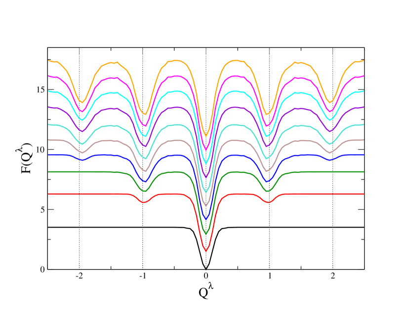
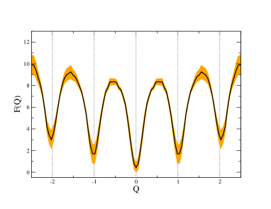
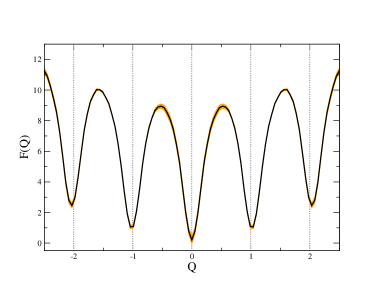
In Fig. 1 we show the metadynamics bias potential averaged over progressively larger number of MC sweeps. As the simulation proceeds, the minima are iteratively filled, until all the five minima shown in figure are explored, and the bias potential starts growing evenly in all the $Q$ range. At this point, the free energy estimator $V_{G}(q,t)$ can be considered converged. Since the instantaneous value of $V_{G}(q,t)$ is subject to fluctuations, in order to extract the free energy and its statistical error, we average $V_{G}(q,t)$ after convergence, namely after 10k HMC sweeps for the example in Figure. In Fig. 2 the reconstructed average free energy of the topological charge $F\left(Q^{\lambda}\right)$ and its statistical uncertainty, shown as a (orange) band, estimated by dividing the Monte Carlo history after equilibration in $n_{p}=4$ different intervals and estimating the standard deviation of the $n_{P}$ measures. In the bottom panel we compare the metadynamics result with $-log(P(Q^{\lambda}))$ estimated in a standard HMC run. Remarkably, the two estimates are fully consistent within the small error bars, indicating that metadynamics allows computing reliably the probability distribution of the charge.

Figure 2: Top: The free energy of the smeared topological charge $F\left(Q^{\lambda}\right)$ estimated by metadynamics and its statistical uncertainty, shown as a (orange) band at $\beta=0.70$ with $L=62$. The average is performed either over 30k sweeps (top left) or over 300k sweeps (top right). Bottom: comparison between the free energy $F\left(Q^{\lambda}\right)$ estimated by metadynamics and $-log(P(Q))$ estimated by the standard HMC. The error on HMC results is not shown.

The most important effect of the metadynamics bias is reducing the autocorrelation time of the observables by orders of magnitude. In Fig. 3 we show the (fictitious) time autocorrelation function for the magnetization and topological charge for the standard HMC run and for the metadynamics run. For comparison, we have chosen for these figures a value of $\beta$ and of the lattice size $L$ equal to one of the runs presented in Ref. Campostrini:1992ar (see also Rossi:1993nz ). The improvement is significant: by fitting the exponential decrease of the autocorrelation functions we find $\tau_{Q}=155000\pm 10000$ in the HMC run, whereas the corresponding value for the metadynamics run is $\tau_{Q}=5600\pm 1000$. In both cases we find $\tau_{m}=50\pm 10$. A related quantity is the transition probability per unit time between two different topological sectors, $\nu$. This quantity is defined as the number of jumps between two different values of $Q^{g}$ divided by the total number of sweeps. For the two runs corresponding to Fig. 4, we have $\nu=4.98\cdot 10^{-5}$ with the HMC and $\nu=2.24\cdot 10^{-3}$ for metadynamics respectively.

Figure 3: (a) and (b) Time autocorrelation functions in logarithmic x-scale for the magnetization and the topological charge. The results correspond to $\beta=0.75$ and $L=60$, for which $E=0.6872601(25)$, $\xi_{G}=5.160(3)$ and $L/\xi_{G}\sim 11.63$.

Figure 4: (a) and (b) Topological charge as a function of the number of sweeps with the standard HMC and metadynamics respectively at $\beta=0.75$ and $L=60$. In the calculation of $\nu$ we have conventionally eliminated jumps in which the system returns to the original value of the topological charge in less than 10 sweeps.

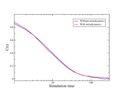
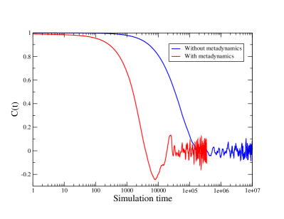
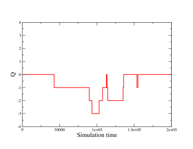
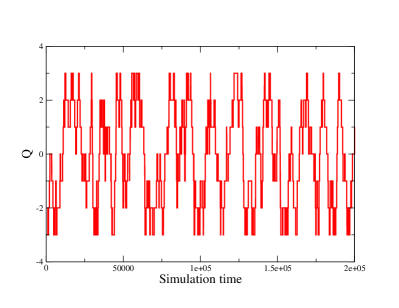
One of the main results of this paper is the reconstructed free energy, Fig. 2, at different values of the coupling $\beta$ and of the volume. Although the specific form of the free energy depends on the definition of $Q^{\lambda}$, it contains some important physical information. $F(Q)$ is very well approximated by the function

$$F(Q)=A\,Q^{2}+b\,\sin^{2}(\pi Q),$$ (26)

where $A$ and $b$ are numerical constants which in general, at fixed $N$, depend on $L$ and $\beta$.

As an example we fitted the effective potential reported in the top-left panel of Fig. 2 relative to $\beta=0.70$ with $L=62$. Taking $c=0$, the results of the fit, in the metadynamics case, are $A=0.20\pm 0.06$ and $B=4.38\pm 0.10$, with a $\chi^{2}/dof~{}1$. By using the relation $A\sim 1/(2\chi_{t}V)$, this corresponds to $\chi_{t}=(6.50\pm 1.9)\times 10^{-4}$ well compatible with the results given in Tab. LABEL:tab:twob for $\beta=0.70$ and $L=62$. The coefficient $b$ is related to the tunneling probability of the system between different topological sectors. Since most of the transitions occur with $\Delta Q=\pm 1$, we expect that $b\sim\kappa\exp[S_{I}]$, where $\kappa$ is an entropy factor which increases with the volume and $S_{I}$ is the one-instanton action $S_{I}=2\pi N\beta$.

IV.2 The central question: Towards the continuum limit

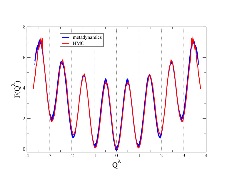
In order to demonstrate that the approach presented in this work allows addressing efficiently the problem of topological trapping, we now discuss the scaling of the autocorrelation time as a function of the lattice spacing $a\sim\xi_{G}^{-1}$, namely of $\xi_{G}$, and of the physical volume $L/\xi_{G}$. In Fig. 5 and Tab. C we display the dependence of $\nu$ on $\xi_{G}$ with HMC and metadynamics at several values of $L/\xi_{G}$.

Figure 5: Scaling of the frequency $\nu$ as a function of $\xi_{G}$ with metadynamics (dashed) and HMC(full line) for three different values of $L/\xi_{G}$. In the case of the standard HMC, for $a\xi_{G}\gtrsim 9$ the changes of the topological sector are so rare that only an upper limit can be estimated.

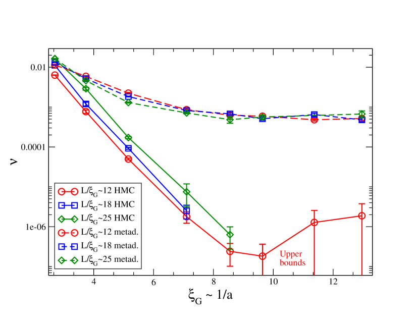
As expected, because of entropy, in the standard HMC $\nu$ is an increasing function of the lattice size, and this corresponds to an increase in the dispersion of the topological charge, namely of $\langle Q^{2}\rangle$. At larger values of $\beta$, as we proceed toward the continuum limit, with the standard HMC, $\nu$ decreases exponentially as a function of the correlation length $\xi_{G}$ DelDebbio:2002xa ; DelDebbio:2004xh , so that for $a\xi_{G}\gtrsim 9$ the changes of the topological sector are so rare that only an upper limit for $\nu$ can be provided.
The fact that the system is locked in a given topological sector may severely bias the lattice predictions for several important physical quantities, in primis the topological susceptibility. The apparent small errors with HMC for the topological susceptibility at large values of $\beta$, for example at $\beta=0.80$, with $L=80$, see Tab. LABEL:tab:twoa, are illusory because they refer to an average taken essentially at fixed topological charge and thus its value is affected by a systematic error. This is dramatically clear by comparing the values of the renormalization group invariant product $\chi_{t}\xi_{G}^{2}$ in the last column of Tab. LABEL:tab:twoa and LABEL:tab:twob. $\beta=0.8$ is just the largest value at which we could made a comparison between standard HMC and metadynamics, since above that it is impossible to get sensible results for the topological susceptibility using HMC. Indeed, with the standard HMC the number of sweeps necessary to get the correct results increases exponentially with $\beta$ while in metadynamics increases only linearly.

The behavior observed with the HMC is to be contrasted with the results obtained with metadynamics (corrected for the bias using eq. 25) since in this case $\nu$ is sensibly flatter, and the simulation spans all the possible sectors of $Q$ allowing to produce reliable results.

We first analyze the scaling of the performances with the volume. It is known that in HMC the autocorrelation time of topological charge does not increase with the volume, as the increased tunneling rate (due to larger entropy) compensates the larger range of topological charges to explore. In metadynamics it is a priori not clear how the mechanism of tunnelling is affected by the volume. We note empirically (see Fig. 5) that the tunnelling rate does not change with the volume, so one would expect that the algorithm efficiency degrades (mildly) with the volume. This is partially sustained from the observation of the errors reported on the last two columns of Tab. LABEL:tab:twob. Nonetheless we remark that, no matter which volume is chosen, we still expect metadynamics to scale better with the lattice spacing than HMC. This means that for any physical volume there is a critical lattice spacing below which using metadynamics is convenient.

The final issue that we have to address is the scaling of the error of observable quantities measured in the metadynamics simulations. As we proceed to the continuum limit, the weight of configurations with non integer $Q^{\lambda}$ decreases, but the system keeps exploring all values $Q^{\lambda}\in[-Q^{thr},+Q^{thr}]$ with equal probability after that the bias potential has converged. The unbiased expectation value is recovered by the reweighting procedure of eq. 25. The impact of the reweighting can be estimated modelling the scaling of the bias potential with the lattice spacing. Assuming that in the parametrization of eq. 26 the coefficient $b$, corresponding to the height of the barriers, grows approximately as $1/a$, one expects a mild increase of the error due to reweighting. By comparing Tabs. LABEL:tab:twoa and  LABEL:tab:twob one is comforted by observing that at small $\beta$ (where HMC simulations are reliable) the errors for $\xi_{G}$, $E$ and $\chi_{m}$ obtained with metadynamics are comparable with those obtained with HMC, and increase very slowly with $\beta$, not faster than the standard HMC.

For the case of the renormalization invariant combination $\chi_{t}\xi_{G}^{2}$ we observe that in the case of HMC the errors growth relatively less than with metadynamics, but the value drops dramatically at large $\beta$ due to the freezing of the topological charge. With metadynamics we find similar values across the whole range of explored lattice spacings, signaling that the algorithm samples correctly the distribution of the topological charge, as opposed to HMC.

In spite of the great effort undertaken in the past DelDebbio:2002xa ; DelDebbio:2004xh ; Flynn:2015uma even for the HMC algorithm it is not clear yet whether the topological modes are affected by exponential or power-like slowing down. In this first work we do not aim at determining accurately the scaling properties of our current implementation of metadynamics. We can however note that the observed growth of the error on the topological susceptibility as a function of the lattice spacing is compatible with a power law divergence of topological autocorrelation time, with an exponent that we estimate to be $2\div 3$. This has to be compared with the pure HMC simulations, for which the exponent of the power-like ansatz has steadily been suggested to be close to 5. We consider this a substantial improvement, that allows already to have reliable results at $\beta$ much larger that the HMC. Based on previous experience bias_exchange , further improvement might be obtained including a larger set of collective variables to the algorithm, possibly coupling including in the bias other slow modes.

Table A: Parameters and measured quantities of the standard HMC simulation. All the quantities are measured every 5 sweeps except the energy and the topological charge which are measured every sweep.

$\beta=\frac{1}{gN}$	$N_{s}$	$L$	$\xi_{G}$	$L/\xi_{G}$	$E$	$\chi_{m}\times 10^{4}$	$\chi_{t}\times 10^{4}$	$\chi_{t}\xi_{G}^{2}\times 10^{4}$
0.65	3M	32	2.7009(13)	11.848(15)	0.799324(9)	12.182(3)	11.66(18)	85.1(1.3)
	3M	46	2.7024(19)	17.022(12)	0.799352(8)	12.148(3)	11.91(26)	87(2)
	3M	64	2.7075(23)	23.64(2)	0.799357(4)	12.147(2)	11.6(3)	84.9(2.2)
0.70	3M	44	3.748(3)	11.739(8)	0.739053(4)	19.613(8)	5.56(24)	78(3)
	3M	62	3.742(3)	16.57(5)	0.739072(4)	19.545(4)	5.93(14)	83(2)
	3M	88	3.743(4)	23.508(27)	0.739066(3)	19.543(5)	5.88(26)	82(4)
0.75	3M	60	5.169(7)	11.608(16)	0.687256(6)	31.890(31)	2.5(3)	67(8)
	3M	84	5.154(8)	16.299(24)	0.687270(6)	31.725(21)	3.7(5)	97(13)
	3M	120	5.152(16)	23.28(7)	0.6872678(21)	31.723(18)	2.9(5)	78(13)
0.80	3M	80	7.141(13)	11.203(20)	0.642261(4)	52.48(6)	0.74(12)	38(6)
	3M	114	7.102(8)	16.051(18)	0.6422752(22)	52.120(23)	0.29(6)	15(3)
	3M	160	7.075(20)	22.61(6)	0.6422784(15)	52.044(22)	0.25(8)	13(4)

Table B: Parameters and measured quantities of the metadynamics simulation.

$\beta=\frac{1}{gN}$	$N_{s}$	$L$	$\xi_{G}$	$L/\xi_{G}$	$E$	$\chi_{m}\times 10^{4}$	$\chi_{t}\times 10^{4}$	$\chi_{t}\xi_{G}^{2}\times 10^{4}$
0.65	3M	32	2.7000(20)	11.852(9)	0.799310(14)	12.181(4)	11.44(14)	83.4(1.1)
	3M	46	2.6994(24)	17.041(15)	0.799366(6)	12.1448(29)	11.83(19)	86.2(1.4)
	3M	64	2.702(4)	23.696(36)	0.799354(6)	12.146(3)	11.32(15)	82.6(1.1)
0.70	3M	44	3.743(4)	11.756(12)	0.739049(10)	19.608(10)	5.68(11)	79.6(1.5)
	3M	62	3.742(6)	16.576(16)	0.739069(6)	19.550(7)	5.66(12)	79.2(1.7)
	3M	88	3.750(5)	23.47(3)	0.739071(4)	19.539(4)	5.68(25)	80(3)
0.75	3M	60	5.149(7)	11.653(15)	0.687281(7)	31.795(21)	3.01(7)	79.8(1.8)
	3M	84	5.141(7)	16.339(23)	0.687270(5)	31.717(13)	2.91(14)	77(3)
	3M	120	5.183(11)	23.15(5)	0.687272(4)	31.735(10)	3.2(3)	86(8)
0.80	3M	80	7.079(7)	11.302(11)	0.642289(5)	52.141(30)	1.78(19)	87(10)
	3M	114	7.098(19)	16.06(4)	0.642288(4)	51.98(4)	1.80(23)	89(12)
	3M	160	7.072(19)	22.62(6)	0.6422797(26)	51.971(22)	1.79(20)	88(10)
0.85	3M	108	9.672(18)	11.166(21)	0.602879(5)	85.91(8)	1.00(16)	91(15)
0.875	3M	126	11.073(21)	11.379(21)	0.584949(4)	110.72(14)	0.69(16)	77(20)
0.9	3M	148	13.32(4)	11.112(30)	0.5680742(29)	143.28(22)	0.42(23)	73(41)

$\beta$	$L$	$\nu$ HMC	$\nu$ metadynamics
0.65	12	$(6.4\pm 0.1)\times 10^{-3}$	$(11.5\pm 0.4)\times 10^{-3}$
0.70	12	$(7.7\pm 0.8)\times 10^{-4}$	$(5.9\pm 0.2)\times 10^{-3}$
0.75	12	$(5.0\pm 0.3)\times 10^{-5}$	$(2.2\pm 0.1)\times 10^{-3}$
0.80	12	$(1.8\pm 0.6)\times 10^{-6}$	$(8.7\pm 0.5)\times 10^{-4}$
0.83	12	$(2.4\pm 1.4)\times 10^{-7}$	$(6.2\pm 0.2)\times 10^{-4}$
0.65	18	$(11.1\pm 0.1)\times 10^{-3}$	$(13.4\pm 0.2)\times 10^{-3}$
0.70	18	$(1.1\pm 0.1)\times 10^{-3}$	$(5.2\pm 0.1)\times 10^{-3}$
0.75	18	$(9.3\pm 0.5)\times 10^{-5}$	$(1.84\pm 0.04)\times 10^{-3}$
0.80	18	$(2.5\pm 0.9)\times 10^{-6}$	$(8.2\pm 0.3)\times 10^{-4}$
0.65	25	$(16.2\pm 0.2)\times 10^{-3}$	$(16.4\pm 0.2)\times 10^{-3}$
0.70	25	$(2.9\pm 0.2)\times 10^{-3}$	$(4.62\pm 0.06)\times 10^{-3}$
0.75	25	$(1.7\pm 0.1)\times 10^{-4}$	$(1.30\pm 0.04)\times 10^{-3}$
0.80	25	$(7.5\pm 4.3)\times 10^{-6}$	$(7.1\pm 0.3)\times 10^{-4}$

Table C: Values of the frequency $\nu$ as a function of the coupling for different physical volumes. In the table we only give the values of $\nu$ that have been reliably determined, excluding those corresponding to $\beta$ so large that, in the case of HMC, only an upper bound can be given.

V Conclusions

In this paper we have shown that the metadynamics approach laio2002escaping ; laio2 can be used to simulate $CP^{N-1}$ improving dramatically the problem of the slowing down observed in numerical simulations for quantities related to the topological charge. In particular we have studied the $N=21$ case, showing that we are able to reconstruct the free energy of the topological charge, $F(Q)$, as a function of the coupling and of the volume.

The much reduced slowing down allows us to study a range of $\beta$ much larger than that available with ordinary HMC. Further improvement might be obtained by biasing a larger set of collective variables.

It seems straightforward to extend the general method exposed in this paper to the case of QCD. It will be interesting to investigate whether metadynamics will also work in this case.

The possibility of measuring of $F(Q)$ suggests that we can further improve the efficiency of the algorithm by using the information about its form as obtained in a preliminary run, cfr. eq. (26). This would allow simulating our system by using as importance sampling the knowledge of free energy itself added to the original action of our theory.

The knowledge of the free energy of the topological charge ($Q^{\lambda}$ in our case) is very important for the study of relevant physical quantities. Actually, if we know the free energy of the topological charge, then we can compute the expectation value of any physical quantity at arbitrary values of $\theta$-vacuum, and not only close to the origin, by simply averaging them with the appropriate weight $\sim\cos(\theta Q)\,e^{-F(Q)}$, where we used the property that $F(-Q)=F(Q)$. Metadynamics might thus also offer a solution to the difficulties encountered in simulating theories with complex actions (for example QCD with a non zero $\theta$ term or at finite chemical potential).

Appendix A

Taking inspiration from QCD we define recursively the $\left(n+1\right)$-level stout smeared link $\lambda_{m;\mu}^{\left(n+1\right)}$ in terms of the $n$-level stout smeared link $\lambda_{m;\mu}^{n}$ as

$$\lambda_{m;\mu}^{\left(n+1\right)}=e^{iQ_{m;\mu}^{\left(n\right)}}\lambda_{m;\mu}^{\left(n\right)}\,,$$

where

$$Q_{m;\mu}^{\left(n\right)}={\rm Im}\left(\rho S_{m;\mu}^{\left(n\right)}\lambda^{\left(n\right)}_{m;\mu}\right)\,,$$

and $S_{m;\mu}^{\left(n\right)}$ are the staples :

$$S^{\left(n\right)}_{m;\mu}=\sum_{v\neq\mu}\left[\lambda^{\left(n\right)}_{m;\nu}\lambda^{\left(n\right)}_{m+\hat{\nu};\mu}\lambda^{\left(n\right)*}_{m+\hat{\mu};\nu}+\lambda^{\left(n\right)*}_{m-\hat{\nu};\nu}\lambda^{\left(n\right)}_{m-\hat{\nu};\mu}\lambda^{\left(n\right)}_{m+\hat{\nu}+\hat{\mu};\nu}\right]\,,$$

being $\rho$ a small real number. The recursive procedure is based on the $0$-level stout smeared links, that are nothing but the original (non-smeared) ones .

As an effect of the exponentiation, the level-1 link results to be the average of the original link and the collection of all the infinite paths surrounding the two nearby $1\times 1$ plaquettes:

$\boldsymbol{=}$ $\boldsymbol{+}$$\frac{\rho}{2}$ $\Big{\{}$ $\boldsymbol{+}$ …$\Big{\}}$ .

The definition is recursive and the $n$-level smeared link will involve contribution of links as far as $d\leq n$ sites (each of them damped by a power $\rho^{d}$). Averaging a link with paths built in terms of its neighbors suppresses ultraviolet fluctuations, and reduces the noise in observables built in terms of the links. The parameters $\rho$ and $n$ can be tuned separately, but what indeed matters is the product $\rho\,n$. We found it convenient to use $n=2$ and vary linearly $\rho$ as a function of $\beta$ ($\rho=0.08$ at $\beta=0.65$ and $\rho=0.13$ at $\beta=0.90$) which allows to separate the distribution probabilities of $Q^{\lambda}$ for different topological sectors as explained in Sec. III.

References

- (1) P. Rossi and E. Vicari, Phys. Rev. D 48 (1993) 3869 [hep-lat/9301008].
- (2) L. Del Debbio, H. Panagopoulos and E. Vicari, JHEP 0208 (2002) 044 [hep-th/0204125].
- (3) L. Del Debbio, G. M. Manca and E. Vicari, Phys. Lett. B 594 (2004) 315 [hep-lat/0403001].
- (4) M. Luscher, PoS LATTICE 2010 (2010) 015 [arXiv:1009.5877 [hep-lat]].
- (5) S. Schaefer et al. [ALPHA Collaboration], Nucl. Phys. B 845 (2011) 93 [arXiv:1009.5228 [hep-lat]].
- (6) M. Luscher and S. Schaefer, JHEP 1107 (2011) 036 [arXiv:1105.4749 [hep-lat]].
- (7) A. Chowdhury, A. Harindranath, J. Maiti and P. Majumdar, JHEP 1402 (2014) 045 [arXiv:1311.6599 [hep-lat]].
- (8) R. C. Brower et al. [LSD Collaboration], Phys. Rev. D 90 (2014) 1, 014503 [arXiv:1403.2761 [hep-lat]].
- (9) J. Flynn, A. Juttner, A. Lawson and F. Sanfilippo, arXiv:1504.06292 [hep-lat].
- (10) G. P. Engel and S. Schaefer, Comput. Phys. Commun. 182 (2011) 2107 [arXiv:1102.1852 [hep-lat]].
- (11) G. Veneziano, Nucl. Phys. B159 , 213 (1979).
- (12) E. Witten, Nucl. Phys.B156, 269 (1979).
- (13) L. Del Debbio, L. Giusti and C. Pica, Phys. Rev. Lett. 94 (2005) 032003 [hep-th/0407052].
- (14) M. Cè, C. Consonni, G. P. Engel and L. Giusti, Phys. Rev. D 92, no. 7, 074502 (2015) [arXiv:1506.06052 [hep-lat]].
- (15) G. M. Shore, Lect. Notes Phys. 737 (2008) 235 [hep-ph/0701171].
- (16) C. A. Aidala, S. D. Bass, D. Hasch and G. K. Mallot, Rev. Mod. Phys. 85 (2013) 655 [arXiv:1209.2803 [hep-ph]].
- (17) C. Marchand, DOI: 10.3204/DESY-PROC-2012-02/20 Conference: C12-03-26.1, p.27-36.
- (18) J. Mulders, Prog. Part. Nucl. Phys. 55, 243 (2005).
- (19) P. de Forcrand, J. E. Hetrick, T. Takaishi and A. J. van der Sijs, Nucl. Phys. Proc. Suppl. 63 (1998) 679 [hep-lat/9709104].
- (20) A. Ramos, PoS LATTICE 2012, 193 (2012) [arXiv:1212.3800 [hep-lat]].
- (21) G. McGlynn and R. D. Mawhinney, PoS Lattice 2013, 027 (2014) [arXiv:1311.3695 [hep-lat]].
- (22) U. Gerber, I. Bautista, W. Bietenholz, H. Mejía-Díaz and C. P. Hofmann, PoS LATTICE 2014, 320 (2014) [arXiv:1410.0426 [hep-lat]].
- (23) M. G. Endres, R. C. Brower, W. Detmold, K. Orginos and A. V. Pochinsky, arXiv:1510.04675 [hep-lat].
- (24) A. S. Gambhir and K. Orginos, PoS LATTICE 2014, 043 (2015) [arXiv:1506.06118 [hep-lat]].
- (25) A. Dromard, W. Bietenholz, U. Gerber, H. MejÃa-DÃaz and M. Wagner, arXiv:1510.08809 [hep-lat].
- (26) A. Laio, M. Parrinello, Proceedings of the National Academy of Sciences, 2002, 99.20: 12562-12566.
- (27) A. Laio and F.L. Gervasio, Rep. Prog. Phys. 71, 126601, 2008
- (28) F. Wang, F. and D. P. Landau Phys. Rev. Lett. 86 (2001) 2050. [arXiv:cond-mat/0011174]
- (29) Y. Crespo, F. Marinelli, F. Pietrucci, A. Laio, Physical Review E, 81, 055701 (2010).
- (30) P. Di Vecchia, A. Holtkamp, R. Musto, F. Nicodemi and R. Pettorino, Nucl. Phys. B 190 (1981) 719.
- (31) B. Berg and M. Luscher, Nucl. Phys. B 190 (1981) 412.
- (32) M. Campostrini, P. Rossi and E. Vicari, Phys. Rev. D 46 (1992) 2647.
- (33) S. Piana, A. Laio, A bias-exchange approach to protein folding Journal of Physical Chemistry B, 111, 4553 (2007).
- (34) C. Bonati and M. D’Elia, Phys. Rev. D 89 (2014) 105005 [arXiv:1401.2441 [hep-lat]].
- (35) M. Albanese et al. [APE Collaboration], Phys. Lett. B 192 (1987) 163.
- (36) A. Hasenfratz and F. Knechtli, Phys. Rev. D 64 (2001) 034504 [hep-lat/0103029].
- (37) C. Morningstar and M. J. Peardon, Phys. Rev. D 69 (2004) 054501 [hep-lat/0311018].