Exact triangles for $\mathop{\mathit{SO}}(3)$ instanton homology of webs

1 Introduction

Let $K\subset\mathbb{R}^{3}$ be an unoriented web, i.e. an embedded trivalent graph whose local model at the vertices is that of three arcs meeting with distinct tangent directions. In a previous paper [6], the authors defined an invariant $J^{\sharp}(K)$ for such webs, as an $\mathop{\mathit{SO}}(3)$ instanton homology with coefficients in the field $\mathbb{F}=\mathbb{Z}/2$. This instanton homology is functorial for foams, which are singular cobordisms between webs. The construction of $J^{\sharp}(K)$ closely resembles an invariant $I^{\sharp}(K)$ defined earlier for knots and links in [8]. Knots and links are webs without vertices; but even for these, $I^{\sharp}(K)$ and $J^{\sharp}(K)$ are different, because $I^{\sharp}(K)$ was defined using $\mathop{\mathit{SU}}\nolimits(2)$ representation varieties, while $J^{\sharp}(K)$ uses $\mathop{\mathit{SO}}(3)$. Our conventions and definitions are briefly recalled in section 2.

This paper is a continuation of [6] and establishes a type of skein relation (an exact triangle) for $J^{\sharp}$. The main result concerns three webs $L_{2}$, $L_{1}$, $L_{0}$ which differ only inside a ball, as shown:

$$L_{2}={\begin{array}[]{c}\raisebox{-2.5pt}{\includegraphics[width=34.2537pt]{figures/Graph-Xbar}}\end{array}},\qquad L_{1}={\begin{array}[]{c}\raisebox{-2.5pt}{\includegraphics[width=34.2537pt]{figures/Graph-H}}\end{array}},\qquad L_{0}={\begin{array}[]{c}\raisebox{-2.5pt}{\includegraphics[width=34.2537pt]{figures/Graph-I}}\end{array}}.$$ (1)

There are standard foam cobordisms between these (see section 3 for a fuller description):

$$\cdots\longrightarrow{\begin{array}[]{c}\raisebox{-2.5pt}{\includegraphics[width=34.2537pt]{figures/Graph-Xbar}}\end{array}}\longrightarrow{\begin{array}[]{c}\raisebox{-2.5pt}{\includegraphics[width=34.2537pt]{figures/Graph-H}}\end{array}}\longrightarrow{\begin{array}[]{c}\raisebox{-2.5pt}{\includegraphics[width=34.2537pt]{figures/Graph-I}}\end{array}}\longrightarrow{\begin{array}[]{c}\raisebox{-2.5pt}{\includegraphics[width=34.2537pt]{figures/Graph-Xbar}}\end{array}}\longrightarrow\cdots$$

We then have:

Theorem 1.1.

The sequence of $\mathbb{F}$-vector spaces obtained by applying $J^{\sharp}$ to the above sequence of webs and foams is exact:

$$\cdots\longrightarrow J^{\sharp}(L_{2})\longrightarrow J^{\sharp}(L_{1})\longrightarrow J^{\sharp}(L_{0})\longrightarrow J^{\sharp}(L_{2})\longrightarrow\cdots$$

There is a variant of this exact triangle. Consider three webs differing in the ball as in the following diagrams:

$$K_{2}={\begin{array}[]{c}\raisebox{-2.5pt}{\includegraphics[width=34.2537pt]{figures/Graph-X}}\end{array}},\qquad K_{1}={\begin{array}[]{c}\raisebox{-2.5pt}{\includegraphics[width=34.2537pt]{figures/Graph-Res1}}\end{array}},\qquad K_{0}={\begin{array}[]{c}\raisebox{-2.5pt}{\includegraphics[width=34.2537pt]{figures/Graph-Res0}}\end{array}}.$$

Again, there are standard cobordisms between these. In [8], we established an exact triangle in $I^{\sharp}$ relating these three. The corresponding sequence of vector spaces $J^{\sharp}(K_{i})$ do not form an exact triangle. Instead, there is an exact triangle involving $L_{i+2}$, $K_{i+1}$ and $K_{i}$, for each $i$ (with the indices interpreted cyclically modulo $3$). Thus:

Theorem 1.2.

For each $i=0,1,2$, we have an exact sequence of $\mathbb{F}$-vector spaces,

$$\cdots\longrightarrow J^{\sharp}(L_{i+2})\longrightarrow J^{\sharp}(K_{i+1})\longrightarrow J^{\sharp}(K_{i})\longrightarrow J^{\sharp}(L_{i+2})\longrightarrow\cdots,$$

in which the maps are obtained by applying $J^{\sharp}$ to standard foam cobordisms.

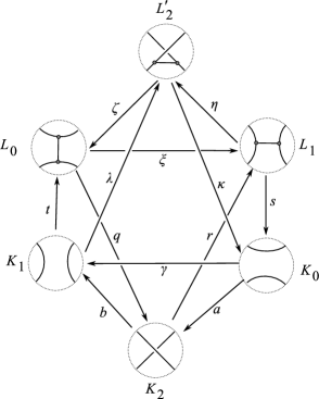
Figure 1: An octahedral diagram whose faces are four exact triangles and four commutative triangles.

The four exact triangles contained in the two theorems above can be arranged as four of the triangular faces in an octahedral diagram, a particular realization of the diagram for the octahedral axiom for a triangulated category. In the diagram, Figure 1, the top vertex $L^{\prime}_{2}$ has a crossing of a different sign from the picture of $L_{2}$. The exact triangles in this octahedron are

$$\cdots \longrightarrow J^{\sharp}(K_{2})\longrightarrow J^{\sharp}(K_{1})\longrightarrow J^{\sharp}(L_{0})\longrightarrow J^{\sharp}(K_{2})\longrightarrow\cdots$$

$$\cdots \longrightarrow J^{\sharp}(K_{2})\longrightarrow J^{\sharp}(L_{1})\longrightarrow J^{\sharp}(K_{0})\longrightarrow J^{\sharp}(K_{2})\longrightarrow\cdots$$

$$\cdots \longrightarrow J^{\sharp}(K_{0})\longrightarrow J^{\sharp}(K_{1})\longrightarrow J^{\sharp}(L^{\prime}_{2})\longrightarrow J^{\sharp}(K_{0})\longrightarrow\cdots$$

$$\cdots \longrightarrow J^{\sharp}(L_{0})\longrightarrow J^{\sharp}(L_{1})\longrightarrow J^{\sharp}(L^{\prime}_{2})\longrightarrow J^{\sharp}(L_{0})\longrightarrow\cdots.$$

The last two are duals of exact triangles in Theorems 1.2 and 1.1 respectively. The other four faces of octahedron become commutative diagrams of $\mathbb{F}$-vector spaces on applying $J^{\sharp}$. For example, the triangle

is a commutative diagram. Finally, the two different composites from $K_{2}$ to $L^{\prime}_{2}$,

$${\begin{array}[]{c}\raisebox{-2.5pt}{\includegraphics[width=34.2537pt]{figures/Graph-X}}\end{array}} \longrightarrow{\begin{array}[]{c}\raisebox{-2.5pt}{\includegraphics[width=34.2537pt]{figures/Graph-H}}\end{array}}\longrightarrow{\begin{array}[]{c}\raisebox{-2.5pt}{\includegraphics[width=34.2537pt]{figures/Graph-Xbardag}}\end{array}}$$

$${\begin{array}[]{c}\raisebox{-2.5pt}{\includegraphics[width=34.2537pt]{figures/Graph-X}}\end{array}} \longrightarrow{\begin{array}[]{c}\raisebox{-2.5pt}{\includegraphics[width=34.2537pt]{figures/Graph-Res1}}\end{array}}\longrightarrow{\begin{array}[]{c}\raisebox{-2.5pt}{\includegraphics[width=34.2537pt]{figures/Graph-Xbardag}}\end{array}},$$

give the same map $J^{\sharp}(K_{2})\to J^{\sharp}(L^{\prime}_{2})$, with a similar (and equivalent) statement about the two composites from $L^{\prime}_{2}$ to $K_{2}$.

Fuller versions of these results are stated in section 3, where we also broaden the scope of the theorems a little by discussing webs embedded in arbitrary oriented $3$-manifolds, rather than in $\mathbb{R}^{3}$.

Acknowledgement.

The authors are very grateful for the support of the Radcliffe Institute for Advanced Study, which provided them with the opportunity to pursue this project together as Fellows of the Institute during the academic year 2013–2014.

2 Review of $\mathop{\mathit{SO}}(3)$ instanton homology

We briefly recall some of the constructions which are described more fully in [6]. If $Z$ is an $n$-dimensional orbifold, and $z\in Z$, then we write $H_{z}$ for the local stabilizer group at $z$. All our orbifolds will be orientable, so $H_{z}$ is a subgroup of $\mathop{\mathit{SO}}(n)$ acting effectively on $\mathbb{R}^{n}$.

Bifolds.

For $m\leq n$, let $H_{m}\subset\mathop{\mathit{SO}}(m)$ be the elementary abelian $2$-group of order $2^{m-1}$ consisting of diagonal matrices of determinant $+1$ whose diagonal entries are $\pm 1$. Regard $H_{m}$ also as a subgroup of $\mathop{\mathit{SO}}(n)$ for $m\leq n$. We call $Z$ an $n$-dimensional bifold if its local stabilizer groups $H_{z}\subset\mathop{\mathit{SO}}(n)$ are conjugate to $H_{m}$ for some $m\leq n$. All our bifolds will be equipped with Riemannian metrics, in the orbifold sense.

Webs and foams.

The underlying topological space of a bifold is a manifold $X$, and the set of points with non-trivial local stabilizer is a codimension-$2$ subcomplex of $X$. In the case of dimension $2$, this subcomplex is a set of points. In the case $n=3$, it is a trivalent graph, which we refer to as a web.

In the case $n=4$, the points with $H_{z}\neq 1$ form a $2$-complex which we call a foam. A foam can have tetrahedral points, where the local stabilizer is $H_{4}$. The set of points with $H_{z}\cong H_{3}$ is a union of arcs and circles: these are the seams, which together with the tetrahedral points comprise a $4$-valent graph. The remainder of the foam is a $2$-manifold whose components are the faces.

A pair $(Y,K)$ consisting of a smooth $3$-manifold and smoothly embedded web can be used to construct a corresponding bifold $\check{Y}$. The same is true for a pair $(X,\Phi)$ consisting of a $4$-manifold and an embedded foam: we may write the corresponding bifold as $\check{X}$. There is a cobordism category in which the objects are closed, oriented $3$-dimensional bifolds $\check{Y}$ with bifold metrics, and in which the morphisms are isomorphism classes of oriented $4$-dimensional bifolds $\check{X}$ with boundary. Equivalently, we have a category in which the objects are $3$-manifolds $(Y,K)$ with embedded webs, and the morphisms are $4$-manifolds $(X,\Phi)$ with embedded foams.

Bifold connections.

By a bifold connection over a bifold $\check{X}$, we mean an $\mathop{\mathit{SO}}(3)$ orbifold vector bundle $E\to\check{X}$ equipped with an orbifold $\mathop{\mathit{SO}}(3)$ connection $A$, subject to the constraint that at each point $x$ where $H_{x}$ has order $2$, the local action of $H_{x}$ on the $\mathop{\mathit{SO}}(3)$ fiber is non-trivial. This condition determines the local model uniquely at other orbifold points. In particular, if $\check{X}$ is $4$-dimensional and $x$ belongs to a seam of the corresponding foam, so that $H_{x}$ is the Klein $4$-group, then the representation of $H_{x}$ on the $\mathop{\mathit{SO}}(3)$ fiber is the inclusion of the standard Klein $4$-group $V\subset\mathop{\mathit{SO}}(3)$.

Marking data.

Bifold connections may have non-trivial automorphisms. For example, if the monodromy group of the connection is the $4$-group $V$, then the automorphism group is also $V$. In order to have objects without automorphisms, we introduce marked bifold connections.

By marking data $\mu$ on a bifold $\check{X}$, we mean a pair $(U_{\mu},E_{\mu})$ consisting of an open set $U_{\mu}$ and an $\mathop{\mathit{SO}}(3)$ bundle $E_{\mu}\to U_{\mu}\cap\check{X}^{o}$ (where $\check{X}^{o}$ is the locus of non-orbifold points). A marked bifold connection is a bifold connection $(E,A)$ on $\check{X}$ together with a choice of an equivalence class of an isomorphism $\sigma$ from $E|_{U_{\mu}\cap\check{X}^{o}}$ to $E_{\mu}|_{U_{\mu}\cap\check{X}^{o}}$. Two isomorphism $\sigma_{1}$ and $\sigma_{2}$ are equivalent if $\sigma_{1}\circ\sigma_{2}^{-1}:E_{\mu}\to E_{\mu}$ lifts to the determinant-$1$ gauge group, i.e. a section of the associated bundle with fiber $\mathop{\mathit{SU}}\nolimits(2)$. The marking data is strong if the automorphism group of every $\mu$-marked bifold connection is trivial. In dimension $3$, a sufficient condition for $\mu$ to be strong is that $U_{\mu}$ contains a point $x$ with $H_{x}=V$ (a vertex of the corresponding web), or that $U_{\mu}\check{X}^{o}$ contains a torus on which $w_{2}(E_{\mu})$ is non-zero.

Instanton homology.

Let $\check{Y}$ be a closed, connected, oriented $3$-dimensional bifold with strong marking data $\mu$. The set of isomorphism classes of $\mu$-marked bifold connections of Sobolev class $L^{2}_{k}$, for large enough $k$, is parametrized by a Hilbert manifold $\mathcal{B}_{k}(\check{Y};\mu)$. Using the perturbed Chern-Simons functional, one constructs a Morse complex, whose homology we call the $\mathop{\mathit{SO}}(3)$ instanton homology. It is defined with coefficients $\mathbb{F}=\mathbb{Z}/2$. We use the notation $J(\check{Y};\mu)$. If $(Y,K)$ is a pair consisting of a $3$-manifold and an embedded web, we similarly write $J(Y,K;\mu)$.

Let $\check{X}$ be an oriented bifold cobordism from $\check{Y_{1}}$ to $\check{Y}_{2}$, let $\nu$ be marking data for $\check{X}$, and let $\mu_{i}$ be the restriction of $\nu$ to $\check{Y}_{i}$. If $\mu_{i}$ is strong, for $i=1,2$, then $(\check{X},\nu)$ gives rise to a linear map

$$J(\check{X};\nu):J(\check{Y}_{1};\mu_{1})\to J(\check{Y}_{2};\mu_{2}).$$

In general, the map which $J$ assigns to composite cobordism may not be the composite map. However, the composition law does hold if the marking data $\nu$ on the two cobordisms satisfies an extra condition. In this paper, our cobordisms will always contain product cobordisms in the neighborhoods of the marking data, and $\nu$ will always be a product $[0,1]\times\mu_{1}$. This restriction is sufficient to ensure that the composition law holds.

The construction of $J^{\sharp}$.

Let $K$ be a compact web in $\mathbb{R}^{3}$. From $K$, we form a new web $K^{\sharp}\subset S^{3}$ as the disjoint union of $K$ and a Hopf link $H$ contained in a ball near the point at infinity. As marking data for $(S^{3},K^{\sharp})$, we take $U_{\mu}$ to be the ball containing $H$, disjoint from $K$, and we take $E_{\mu}$ to have $w_{2}\neq 0$ on the torus which separates the two components of the Hopf link. This marking data is strong. We define

$$J^{\sharp}(K)=J(S^{3},K^{\sharp};\mu).$$

Given a foam cobordism $\Phi\subset[0,1]\times\mathbb{R}^{3}$ from $K_{1}$ to $K_{2}$, we similarly construct a new foam $\Phi^{\sharp}$ as $\Phi\cup([0,1]\times H)$, with marking data $\nu=[0,1]\times\mu$. In this way, $\Phi$ gives rise to a linear map

$$J^{\sharp}(\Phi):J^{\sharp}(K_{1})\to J^{\sharp}(K_{2}).$$

In this way we obtain a functor $J^{\sharp}$ with values in the category of $\mathbb{F}$-vector spaces, from a category whose objects are webs in $\mathbb{R}^{3}$ and whose morphisms are isotopy classes of foams with boundary in intervals $[a,b]\times\mathbb{R}^{3}$.

3 Statement of the results

We state now the version of the Theorem 1.1 that we shall prove. Instead of $\mathbb{R}^{3}$, we consider a closed, oriented $3$-manifold $Y$, and three webs $L_{2}$, $L_{1}$, $L_{0}$ in $Y$ which are identical outside a standard ball $B\subset Y$. As in Theorem 1.1, we suppose that, inside the ball $B$, they look as shown in (1). As with other variants of Floer’s exact triangle, there is more symmetry between the three pictures than immediately meets the eye. The same pictures are drawn from a different point of view in the bottom row of Figure 2, to exhibit the cyclic symmetry between the three. We write $K_{i}$ (as in the introduction) for the web obtained from $L_{i}$ by forgetting the two vertices inside the ball and deleting the edge joining them. Similar picture of the these webs are shown in Figure 3. Let $\mu=(U_{\mu},E_{\mu})$ be strong marking data with $U_{\mu}$ disjoint from $B$. We may regard $\mu$ as marking data for all three of the pairs $(Y,L_{i})$ and all three of the pairs $(Y,K_{i})$.

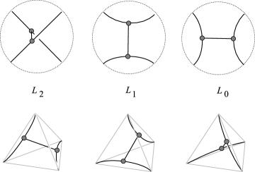
Figure 2: The three webs $L_{i}$, from two different points of view.

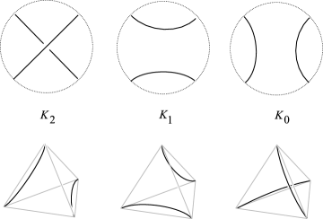
Figure 3: The three webs in $Y$ obtained from the $L_{i}$ by removing an edge.

For each $i$, there is a standard cobordism from $K_{i+1}$ to $K_{i}$ given by a foam $\Sigma(K_{i+1},K_{i})$ in $I\times Y$. (The index $i$ is to be interpreted cyclically.) The cobordism in each case is the addition of a standard $1$-handle. There are also standard cobordisms to and from the $L_{i}$, which we write as $\Sigma(L_{i+1},K_{i})$, $\Sigma(K_{i+1},L_{i})$, and $\Sigma(L_{i+1},L_{i})$. These are all obtained from $\Sigma(K_{i+1},K_{i})$ by adding one or two disks. Pictures of $\Sigma(L_{1},K_{0})$ and $\Sigma(L_{1},L_{0})$ are given in Figure 4. The latter foam has a single tetrahedral point. In the picture of the cobordism from $L_{1}$ to $L_{0}$, we have labeled as $\delta_{1}$ and $\delta_{0}$ the edges of the webs $L_{1}$ and $L_{0}$ which are contained in the interior of the ball. These edges appear on the boundary of disks $\Delta^{+}_{1}$ and $\Delta^{-}_{0}$ in the foam $\Sigma(L_{1},L_{0})$. The tetrahedral point is the unique intersection point $\Delta^{+}_{1}\cap\Delta^{-}_{0}$.

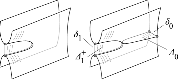
Figure 4: The cobordisms from $L_{1}$ to $K_{0}$ (left) and from $L_{1}$ to $L_{0}$ (right).

The standard cobordisms give maps such as

$$J(I\times Y,\Sigma(L_{i+1},L_{i});\nu):J(Y,L_{i+1};\mu)\to J(Y,L_{i};\mu)$$

where the marking data $\nu$ is the product $I\times\mu$. Thus we have a sequence of maps with period $3$,

$$\dots\to J(Y,L_{2};\mu)\to J(Y,L_{1};\mu)\to J(Y,L_{0};\mu)\to J(Y,L_{2};\mu)\to\cdots$$ (2)

Theorem 3.1.

The above sequence is exact.

As a special case, we can consider webs in $\mathbb{R}^{3}$ and apply the functor $J^{\sharp}$, in which case we deduce the version in the introduction, Theorem 1.1.

There is a similar generalization of Theorem 1.2 in the setting of foams in a $3$-manifold $Y$ with strong marking, whose statement is easily formulated. It will turn out that there is an argument that allows Theorem 1.2 to be deduced from Theorem 1.1 (or, in the more general form, from Theorem 3.1). We will therefore focus on Theorem 3.1 to begin with.

4 Calculations for some connected sums

The quotient of $-\mathbb{C}\mathbb{P}^{2}$ by the action of complex conjugation, $[z_{1},z_{2},z_{3}]\mapsto[\bar{z}_{1},\bar{z}_{2},\bar{z}_{3}]$, is an orbifold $S^{4}$ containing as branch locus the image $R\subset S^{4}$ of $\mathop{\mathbb{R}\mathbb{P}}\nolimits^{2}\subset-\mathbb{C}\mathbb{P}^{2}$. If $L$ is a complex line in $-\mathbb{C}\mathbb{P}^{2}$ defined by real linear equation in the homogeneous coordinates, then the image of $L$ in the quotient is a disk $D$ whose boundary is a real projective line in the branch locus $R$. Given $n$ such lines in $-\mathbb{C}\mathbb{P}^{2}$, say

$$L_{1},\dots,L_{n},$$

we obtain $n$ disks $D_{1},\dots,D_{n}$ in $S^{4}$ whose interiors are disjoint and whose boundaries meet in pairs at points of $R$. The union

$$\Psi_{n}=R\cup D_{1}\cup\cdots\cup D_{n}$$ (3)

is a foam in $S^{4}$. This description does not specify the topology of $\Psi_{n}$ uniquely when $n$ is large, because there are different combinatorial configurations of real projective lines. The cases of most interest to us are $\Psi_{0}$ (which is just the real projective plane $R$ in $S^{4}$, with $R\cdot R=2$), and the foams $\Psi_{1}$, $\Psi_{2}$ and $\Psi_{3}$. The foam $\Psi_{2}$ has a single tetrahedral point where $\partial D_{1}$ meets $\partial D_{2}$ in $R$, while $\Psi_{3}$ has three tetrahedral points.

Lemma 4.1.

The formal dimension of the moduli space of anti-self-dual bifold connections of action $\kappa$ on $(S^{4},\Psi_{n})$ is given by

$$8\kappa-(1-n/2)^{2}.$$

In particular, we have

1. $8\kappa-1$ for $\Psi_{0}$;

2. $8\kappa-1/4$ for $\Psi_{1}$;

3. $8\kappa$ for $\Psi_{2}$;

4. $8\kappa-1/4$ for $\Psi_{3}$;

Proof.

The dimension formula in general is given in [6, Proposition LABEL:prop:dimension], and for foams in $S^{4}$ it reads

$$8\kappa+\chi(\Psi_{n})+\frac{1}{2}(\Psi_{n}\cdot\Psi_{n})-\tau(\Psi_{n})-3,$$

where the self-intersection number $\Psi_{n}\cdot\Psi_{n}$ is computed face-by-face using the framing of the double-cover of the boundary obtained from the seam [6]. For $\Psi_{n}$, there is a contribution of $+2$ from $R\cdot R$ and $-1/2$ from each disk $D_{i}$, so $\Psi_{n}\cdot\Psi_{n}=2-n/2$. The term $\tau$ is the number of tetrahedral points, which is $n(n-1)/2$, and the Euler number $\chi$ is $1+n$. The formula in the lemma follows. ∎

For each of the cases in the previous lemma, we can now consider the non-empty moduli spaces of smallest possible action. For appropriate choices of metrics, we can identify these completely.

Lemma 4.2.

On the bifolds corresponding to $(S^{4},\Psi_{n})$, the smallest-action non-empty moduli spaces of anti-self-dual bifold connections are as follows, for $n\leq 2$.

1. For $n=0$ or $n=2$, there is a unique solution with $\kappa=0$: a flat connection whose holonomy group has order $2$ for $n=0$ and is the Klein $4$-group, $V_{4}$, for $n=2$. The automorphism group of the connection is $O(2)$ (respectively, $V_{4}$), and it is an unobstructed solution in a moduli space of formal dimension $-1$ (respectively, dimension $0$).

2. For $n=1$ and $n=3$, the smallest non-empty moduli spaces have $\kappa=1/32$ and formal dimension $0$. In both cases, with suitable choices of bifold metrics, the moduli space consists of a unique unobstructed solution with holonomy group $O(2)$.

Proof.

The complement $S^{4}\mathord{\setminus}R$ deformation-retracts onto another copy of $\mathop{\mathbb{R}\mathbb{P}}\nolimits^{2}$ in $S^{4}$, which we call $R^{\prime}$ (the image of $R$ under the antipodal map, in a standard construction of $R$). The interiors of the disks $D_{i}$ are the fibers of this retraction. So $S^{4}\mathord{\setminus}\Psi_{n}$ has the homotopy type of $R^{\prime}$ with $n$ punctures. In particular, the fundamental group is $\mathbb{Z}/2$ for $n=0$ and $\mathbb{Z}*\mathbb{Z}$ for $n=2$. For $i=0$ and $2$, the smallest possible action is clearly $\kappa=0$, and we are therefore looking at representations of $\mathbb{Z}/2$ or $\mathbb{Z}*\mathbb{Z}$ in $\mathop{\mathit{SO}}(3)$ sending the standard generators to involutions. In the second case, the two involutions must be distinct and commuting because of the presence of the tetrahedral point where the disks meet. So the flat connections are as described in the lemma. For these bifold connections $A$, we can read off $H^{0}_{A}$ and $H^{1}_{A}$ in the deformation complex by elementary means, and conclude that $H^{2}_{A}=0$ from the dimension formula.

For the case $n=1$, the corresponding bifold admits a double-cover, branched along $R$, for which the total space is $-\mathbb{C}\mathbb{P}^{2}$ containing a complex line $L$ as orbifold locus with cone-angle $\pi$. According to [1, 3], there exists a conformally anti-self-dual bifold metric on $-\mathbb{C}\mathbb{P}^{2}$ with cone-angle $\pi$ along $L$ and positive scalar curvature. This metric is invariant under the action of complex conjugation, and it gives rise to a conformally anti-self-dual metric on the bifold $\check{S}^{4}$ corresponding to $(S^{4},\Psi_{1})$. For such a metric, the obstruction space $H^{2}_{A}$ in the deformation complex of an anti-self-dual bifold connection $A$ is trivial [2, Theorem 6.1], so the moduli space is zero-dimensional and consists of finitely many points, all of which are unobstructed solutions. If $A$ is such a bifold connection, consider its pull-back, $\tilde{A}$, on the double-cover $-\mathbb{C}\mathbb{P}^{2}$, regarded as a bifold with singular locus $L$. The action of $\tilde{A}$ is $1/16$, and the dimension formula shows that the moduli space containing $\tilde{A}$ on this bifold has formal dimension $-1$. Since it is unobstructed, the solution must be reducible, and must therefore be an $\mathop{\mathit{SO}}(2)$ connection, with holonomy $-1$ around the link of $L\subset-\mathbb{C}\mathbb{P}^{2}$. There is a unique such $\mathop{\mathit{SO}}(2)$ solution on $-\mathbb{C}\mathbb{P}^{2}$ with the correct action, and it gives rise to a unique $O(2)$ connection on the original bifold.

In the case $n=3$, the bifold corresponding to $\Psi_{3}\subset S^{4}$ has a smooth $8$-fold cover, which is $-\mathbb{C}\mathbb{P}^{2}$. The covering map is the quotient map for the action of the elementary abelian group of order $8$ acting on $-\mathbb{C}\mathbb{P}^{2}$, generated by the action of complex conjugation and the action of the Klein $4$-group by projective linear transformations. We equip the quotient bifold with the quotient metric of the Fubini-Study metric, so that (as in the case $n=1$) all solutions are unobstructed. A solution of action $1/32$ pulls back to a solution of action $1/4$ on the $8$-fold cover, which must be the unique instanton with holonomy group $\mathop{\mathit{SO}}(2)$ in the $\mathop{\mathit{SO}}(3)$ bundle with Pontryagin number $-1$ on $-\mathbb{C}\mathbb{P}^{2}$. This descends to a unique bifold connection on the quotient. ∎

We use these results about small-action moduli spaces to analyze connected sums in some particular cases. In general, given foams $\Phi\subset X$ and $\Phi^{\prime}\subset X^{\prime}$ with tetrahedral points $t$, $t^{\prime}$ in each, there is a connected sum

$$(X,\Phi)\#_{t,t^{\prime}}(X^{\prime},\Phi^{\prime})$$ (4)

performed by removing standard neighborhoods and gluing together the resulting foams-with-boundary. Similarly, if $s$ and $s^{\prime}$ are points on seams of $\Phi$ and $\Phi^{\prime}$, there is a connected sum

$$(X,\Phi)\#_{s,s^{\prime}}(X^{\prime},\Phi^{\prime}),$$

and there is a connected sum for points $f$ and $f^{\prime}$ in the interiors of faces of the two foams:

$$(X,\Phi)\#_{f,f^{\prime}}(X^{\prime},\Phi^{\prime}),$$

Although our notation does not reflect this, the connected sum is not unique when we summing at a tetrahedral point or a seam. The cause of the non-uniqueness (in the case of the tetrahedral points, for example) is that we have to choose how to identify the $1$-skeleta of the two tetrahedra that arise as the links of $t$ and $t^{\prime}$.

We consider a connected sum at a tetrahedral point in the case that $(X^{\prime},\Phi^{\prime})$ is either $(S^{4},\Psi_{2})$ or $(S^{4},\Psi_{3})$.

Proposition 4.3.

Let $(X,\Sigma)$ be a foam cobordism with strong marking data $\nu$, defining a linear map $J(X,\Sigma,\nu)$. Let $t$ be a tetrahedral point in $\Sigma$.

1. If a new foam $\tilde{\Sigma}$ is constructed from $\Sigma$ as a connected sum

   $$(X,\Sigma)\#_{t,t_{2}}(S^{4},\Psi_{2}),$$

   where $t_{2}$ is the unique tetrahedral point in $\Psi_{2}$, then the new linear map $J(X,\tilde{\Sigma},\nu)$ is equal to the old one.

2. If a new foam $\tilde{\Sigma}$ is constructed from $\Sigma$ as a connected sum

   $$(X,\Sigma)\#_{t,t_{3}}(S^{4},\Psi_{3}),$$

   where $t_{3}$ is any of the three tetrahedral points in $\Psi_{3}$, then the new linear map $J(X,\tilde{\Sigma},\nu)$ is zero.

Proof.

Consider a general connected sum at tetrahedral points, as in equation (4). Let $A$ and $A^{\prime}$ be unobstructed solutions on $(X,\Phi)$ and $(X^{\prime},\Phi^{\prime})$. Let $U_{A}$ and $U_{A^{\prime}}$ be neighborhoods of $[A]$ and $[A^{\prime}]$ in their respective moduli spaces. The limiting holonomy of the connections at the tetrahedral point is the Klein $4$-group $V$, whose commutant in $\mathop{\mathit{SO}}(3)$ is also $V$. So we have moduli spaces of solutions with framing at $t$ and $t^{\prime}$ in which $[A]$ and $[A^{\prime}]$ have neighborhoods $\tilde{U}_{A}$, $\tilde{U}_{A^{\prime}}$, such that $U_{A}=\tilde{U}_{A}/V$ and $U_{A^{\prime}}=\tilde{U}_{A^{\prime}}/V$. Gluing theory provides a model for the moduli space on the connected sum with a long neck, of the form

$$\tilde{U}_{A}\times_{V}\tilde{U}_{A^{\prime}}.$$

If the action of $V$ on $\tilde{U}_{A}$ is free and $U_{A^{\prime}}$ consists of the single point $[A^{\prime}]$, then this local model is a finite-sheeted covering of $U_{A}$ with fiber $V/\Gamma_{A^{\prime}}$, where $\Gamma_{A^{\prime}}\subset V$ is the automorphism group of the solution $A^{\prime}$.

In particular if $A^{\prime}$ is the smallest energy solution on $(S^{4},\Phi_{2})$, then the fiber is a single point, while for $(S^{4},\Phi_{3})$ the fiber is $2$ points. For the case of compact, zero-dimensional moduli spaces on the connected sum, these local models become global descriptions when the neck is long, and we conclude that the moduli space whose point-count defines the map $J(X,\Sigma,\nu)$ is unchanged in the first case and becomes double-covered in the second case. In the second case, the new map is zero because we are working with characteristic $2$. ∎

The next proposition considers similarly the results of connected sum at seam points, where one of the summands is $\Psi_{1}$, $\Psi_{2}$ or $\Psi_{3}$.

Proposition 4.4.

Let $(X,\Sigma)$ be a foam cobordism with strong marking data $\nu$, as in the previous proposition. Let $s$ be a point in a seam of $\Sigma$. For $n=1,2,3$, let $s_{n}$ be a point on a seam of $\Psi_{n}$. If a new foam $\tilde{\Sigma}_{n}$ is constructed from $\Sigma$ as the connected sum

$$(X,\Sigma)\#_{s,s_{n}}(S^{4},\Psi_{n}),$$

then the new linear map $J(X,\tilde{\Sigma}_{n},\nu)$ is equal to the old one in the case $n=2$, and is zero in the case that $n=1$ or $n=3$.

Proof.

The proofs are standard, modeled on the proofs in the previous proposition. ∎

Next we have a proposition about connected sums at points interior to faces of the foams.

Proposition 4.5.

Let $(X,\Sigma)$ be a foam cobordism with strong marking data $\nu$, as in the previous propositions. Let $f$ be a point in the interior of a face of $\Sigma$. Let $f_{n}$ be a point in a face of $\Psi_{n}$. If a new foam $\tilde{\Sigma}_{n}$ is constructed from $\Sigma$ as the connected sum

$$(X,\Sigma)\#_{f,f_{n}}(S^{4},\Psi_{n}),$$

then the new linear map $J(X,\tilde{\Sigma}_{n},\nu)$ is equal to the old one in the case $n=0$, and is zero in all other cases.

Proof.

Again, this is now straightforward. ∎

We consider next a different type of connect sum. Let $\Psi_{2}^{-}$ be the mirror image of $\Psi_{2}$. It has self-intersection number $-1$, Euler number $2$, and one tetrahedral point. In the description of $\Psi_{2}$ in (3), the surface $R$ is divided into two components by the seams of the foam. Let $f_{2}\in R$ be a point in one of those two components.

Proposition 4.6.

Let $(X,\Sigma)$ be a foam cobordism with strong marking data $\nu$. Let $f$ be a point in the interior of a face of $\Sigma$. Let $f_{2}\in\Psi_{2}^{-}$ be as above. If a new foam $\tilde{\Sigma}$ is constructed from $\Sigma$ as the connected sum

$$(X,\Sigma)\#_{f,f_{2}}(S^{4},\Psi^{-}_{2}),$$

then the new linear map $J(X,\tilde{\Sigma},\nu)$ is equal to the old one.

Proof.

Consider a $0$-dimensional moduli space on $(X,\tilde{\Sigma})$. Let $\kappa$ be the action of solutions in this moduli space. If we stretch the neck at the connected sum, and if we obtain in the limit a solution on $(X,\Sigma)$ and a solution on $(S^{4},\Psi_{2}^{-})$, then the action of the solutions on these two summands must be (respectively) $\kappa$ and $0$. The moduli space on $(X,\Sigma)$ with action $\kappa$ is zero-dimensional. The moduli space on $(S^{4},\Psi_{2}^{-})$ with action $0$ consists of a unique $V$-connection $A_{V}$, but the formal dimension of the corresponding moduli space is $-1$, because there is a $1$-dimensional obstruction space $H^{2}(A_{V})$ in the deformation complex. The gluing parameter is $O(2)/V=S^{1}$, so the description of the moduli space on $(X,\Sigma)$ is as the zero-set of a real line bundle $h$ over an $S^{1}$ bundle over the moduli space associated to $(X,\Sigma)$. From this description, we see that

$$J(X,\tilde{\Sigma},\nu)=\epsilon J(X,\Sigma,\nu)$$

where $\epsilon\in\{0,1\}$ is the evaluation of $w_{1}(h)$ on the $S^{1}$ fibers.

To describe $w_{1}(h)$, let us write the $\mathop{\mathit{SO}}(3)$ vector bundle $E$ for the connection $A_{V}$ as a sum of three line bundles,

$$E=L_{0}\oplus L_{1}\oplus L_{2}.$$

In this decomposition, let $i$, $j$, $k$ be the non-identity elements of $V$, chosen to have the form

$$i=\mathop{\mathrm{missing}}{diag}(1,-1,-1),\;\;j=\mathop{\mathrm{missing}}{diag}(-1,1,-1),\;\;k=\mathop{\mathrm{missing}}{diag}(-1,-1,1).$$

Up to conjugacy, the monodromy of $A_{V}$ around the link of the disks $D_{1},D_{2}\subset\Psi^{-}_{2}$ is $i$. The monodromies around the links of the two faces $R\setminus(D_{1}\cup D_{2})$ are $j$ and $k$. The $1$-dimensional vector space $H^{2}(A_{V})$ is spanned a by an $E$-valued form $\omega$ whose values lie in the summand $L_{0}\subset E$ (as follows from the fact that the branched double cover of $S^{4}$ branched over $R$ has $b^{+}=1$). When we form connected sum at a point $f_{2}$ in a face of $\Psi_{2}^{-}$, the obstruction bundle $h$ will be non-trivial on $S^{1}$ if and only if the monodromy of the link at $f_{2}$ acts non-trivially on the summand $L_{0}$ in which $\omega$ lies. Thus $h$ is non-trivial if the monodromy at $f_{2}$ is $j$ or $k$, but $h$ is trivial if the monodromy is $i$. Under the hypotheses of the proposition, $f_{2}$ belongs to one of the faces where the monodromy if $j$ or $k$, so the result follows. ∎

There is a variant of Proposition 4.6 which we will apply in section 8. Consider $S^{4}$ as the union of two standard balls $B^{4}_{+}\cup B^{4}_{-}$. Let $M\subset S^{3}$ be a standard Möbius band whose boundary is an unknot $U$. Let $D^{+}$ and $D^{-}$ be standard disks in $B^{4}_{+}$ and $B^{4}_{-}$ whose boundaries are both $U$. These two disks together with $M$ make a foam,

$$\Psi=D^{+}\cup D^{-}\cup M.$$

If the half-twist in $M$ has the appropriate sign, the self-intersection of the surface real projective plane $R=D^{+}\cup M$ in $S^{4}$ will be $-2$, while $D^{-}\cup M$ has self-intersection $+2$. We can realize $(S^{4},\Psi)$, if we wish, as the $V$-quotient of $S^{2}\times S^{2}$, where one generator of $V$ interchanges the two factors and another generator acts as a reflection on each $S^{2}$ (so that the fixed set of the second generator is $S^{1}\times S^{2}$). Let $f_{\pm}$ be interior points in the faces $D^{\pm}$ of $\Psi$.

Proposition 4.7.

Let $(X,\Sigma)$ be a foam cobordism with strong marking data $\nu$. Let $f$ be a point in the interior of a face of $\Sigma$. Let $\Psi$ be the foam just described, and let $g\in\Psi$ be an interior point of one of the faces of $\Psi$. Let a new foam $\tilde{\Sigma}$ be constructed from $\Sigma$ as the connected sum

$$(X,\Sigma)\#_{f,g}(S^{4},\Psi).$$

Then the new linear map $J(X,\tilde{\Sigma},\nu)$ is equal to the old one if $g$ belongs to $D^{+}$ or to $M$. If $g$ belongs to $D^{-}$, then $J(X,\tilde{\Sigma},\nu)$ is zero.

Proof.

This is an obstructed gluing problem of just the same sort as in the previous proposition. Once again, the branched doubee cover of $S^{4}$ over the surface $R=D^{+}\cup M$ has $b^{+}=1$, and the calculation proceeds as before. (One can alternatively derive this proposition from the previous one by showing that $\Psi$ is a connect sum $\Psi^{-}_{2}\#_{t,t}\Psi_{2}$ at the tetrahedral points.) ∎

5 Topology of the composite cobordisms

As stated in the introduction, the proof of the exact triangle (Theorem 3.1) is very little different from the proof of a corresponding result for the $\mathop{\mathit{SU}}\nolimits(2)$ instanton knot homology $I^{\sharp}$. The first step is to understand the topology of the composites of the cobordisms $\Sigma(L_{i+1},L_{i})$. We shall abbreviate the notation for these cobordisms to just $\Sigma_{i+1,i}$.

Figure 5 shows (schematically) the composite of three consecutive foam cobordisms, from $L_{3}$ to $L_{0}$. The indices are interpreted cyclically, so $L_{3}$ and $L_{0}$ are the same web in $Y$. To explain the picture, in the foam $\Sigma_{1,0}$ pictured in Figure 4, there are two half disks whose removal would leave a standard saddle cobordism from $K_{1}$ to $K_{0}$. When $\Sigma_{2,1}$ and $\Sigma_{1,0}$ are concatenated, two half-disks are joined to form a single disk $\Delta_{1}=\Delta^{-}_{1}\cup\Delta^{+}_{1}$. The triple composite $\Sigma_{3,2}\cup\Sigma_{2,1}\cup\Sigma_{1,0}$ contains two such disks $\Delta_{2}$ and $\Delta_{1}$, as well as two half-disks $\Delta_{3}^{+}$ and $\Delta_{0}^{-}$. These disks are shown shaded in the figure, and in a somewhat schematic manner (because the foams do not embed in $\mathbb{R}^{3}$). If we remove the interiors of these disks from the foam, what remains is a plumbing of Möbius bands, which can be interpreted as a composite cobordism from $K_{3}$ to $K_{0}$ and which appears also as Figure 10 of [8]. We write $\Phi_{3,0}$ for this composite cobordism from $L_{3}$ to $L_{0}$, and $\Phi^{\prime}_{3,0}$ for the complement of the interiors of the disks, as a cobordism from $K_{3}$ to $K_{0}$.

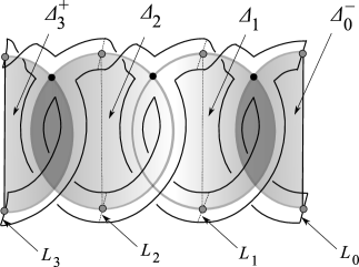
Figure 5: The composite cobordism $\Sigma_{3,2}\cup\Sigma_{2,1}\cup\Sigma_{1,0}$ (portrayed schematically because it is not embedded in $\mathbb{R}^{3}$). The black dots are tetrahedral points. The gray dots are vertices of the webs $L_{i}$.

As explained in [8], a regular neighborhood $B_{1}$ of $\Delta_{1}$ meets $\Phi^{\prime}_{3,0}$ in a Möbius band $M$. The same regular neighborhood meets $\Phi_{3,0}$ in the union

$$M\cup\Delta_{2}^{+}\cup\Delta_{1}\cup\Delta_{0}^{-}.$$ (5)

This union is a foam in the $4$-ball $B_{1}$, and its boundary is the web consisting of the boundary of $M$ and an arc on the boundary of the half-disks $\Delta_{2}^{+}$ and $\Delta_{0}^{-}$. This web is isomorphic to the $1$-skeleton of a tetrahedron, and the foam (5) is the complement of the neighborhood of a tetrahedral point $t_{3}$ in $\Psi_{3}=R\cup D_{1}\cup D_{2}\cup D_{3}$. So we have an isomorphism of pairs,

$$(B_{1},\Phi_{3,0}\cap B_{1})=(S^{4}\mathord{\setminus}N_{t_{3}},\Psi_{3}\mathord{\setminus}N_{t_{3}}),$$ (6)

where $N_{t_{3}}\subset S^{4}$ is a regular neighborhood of $t_{3}$. In particular, we have the following counterpart to Lemma 7.2 of [8].

Lemma 5.1.

The composite cobordism from $(Y,L_{2})$ to $(Y,L_{0})$ formed from the union of the foams $\Sigma_{2,1}$ and $\Sigma_{1,0}$ has the form

$$(I\times Y,V_{2,0})\#_{t,t_{3}}(S^{4},\Psi_{3}),$$

where $V_{2,0}$ is a foam cobordism from $L_{2}$ to $L_{0}$ with a single tetrahedral point $t$.

Consider next the regular neighborhood $B_{2,1}$ of the union of two disks, $\Delta_{2}\cup\Delta_{1}$. The regular neighborhood meets $\Phi^{\prime}_{3,0}$ in a plumbing of two Möbius bands, which is a twice-punctured $\mathop{\mathbb{R}\mathbb{P}}\nolimits^{2}$. There is an isomorphism of pairs,

$$(B_{2,1},\Phi_{3,0}\cap B_{2,1})=(S^{4}\mathord{\setminus}N_{\delta},\Psi_{3}\mathord{\setminus}N_{\delta})$$ (7)

where $\Psi_{3}$ is as in (3) as before, and $N_{\delta}$ is the regular neighborhood of an arc $\delta\subset D_{3}$ which joins the two points $p,q\in\partial D_{3}$ in $\Psi_{3}$. The points $p$ and $q$ lie in the interior of the two arcs which into which $\partial D_{3}$ is divided by the two tetrahedral points.

To examine the picture of (7) further, we note the web that arises as the boundary of $\Phi_{3,0}\cap B_{2,1}$ is also the boundary of the foam $\Omega=N_{\delta}\cap\Psi_{3}$. The foam $\Omega$ consists of two disks which comprise $N_{\delta}\cap R$ together with the rectangle $N_{\delta}\cap D_{3}$.

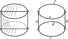
Figure 6: The foam $\Omega$, comprising two disks and a rectangle, and the web $\Gamma$ which is its boundary.

See Figure 6. The foam formed from $\Phi_{3,0}$ removing $\Phi_{3.0}\cap B_{2,1}$ and replacing it with the foam $\Omega$ is isomorphic to the product foam $I\times L_{3}=I\times L_{0}$. Stating this the other way round, we have the following counterpart to Lemma 7.4 of [8].

Lemma 5.2.

The foam $\Phi_{3,0}$ in $I\times Y$ is obtained from the product foam $[0,1]\times L_{0}$ by removing a neighborhood $N$ of the arc $\{1/2\}\times\delta_{0}$ and replacing it with the foam $\Psi_{3}\mathord{\setminus}N_{\delta}$.

6 The chain-homotopies

In order to continue our argument, we streamline our notation. We will then follow closely the argument in [8]. We write simply $Y_{i}$ for the bifold corresponding to the pair $(Y,L_{i})$. We write $X_{1,0}$ for the bifold cobordism from $Y_{1}$ to $Y_{0}$ etc., and we write $X_{3,0}$ (for example) for the composite cobordism from $Y_{3}$ to $Y_{0}$, corresponding to the foam $\Phi_{3,0}$ in $I\times Y$. We write $B_{2,1}$ again for the regular neighborhood of $\Delta_{3}\cup\Delta_{1}$ which we now regard as a bifold ball, contained in the interior of $X_{3,0}$. We also have $B_{1}$, the bifold regular neighborhood of $\Delta_{1}$, which arrange to be contained in the interior of $B_{2,1}$. We similarly have $B_{2}$, the regular neighborhood of $\Delta_{2}$. We write $S_{i}$ for the boundary of $B_{i}$ and $S_{2,1}$ for the regular neighborhood of $B_{2,1}$.

In all, the interior of $X_{3,0}$ contains five $3$-dimensional bifolds,

$$Y_{2},S_{2},S_{1},Y_{1},S_{2,1}.$$ (8)

Arranged cyclically in the above order, each of these five bifolds intersects the ones before and after it, but not the other two. We equip $X_{3,0}$ with a bifold metric which is a product in the two-sided collar of each of the five bifolds, and arrange also that the bifolds meet orthogonally where they intersect. Given a $4$-dimensional bifold $Z$ with boundary, having a metric which is a product metric on a collar of $\partial Z$, we will write $Z^{+}$ for the complete bifold obtained by attaching cylindrical ends to the boundary components:

$$Z^{+}=Z\cup[0,\infty)\times\partial Z.$$

After choosing perturbations, we have a chain complex $(C_{i},D_{i})$ associated to $Y_{i}$, whose homology is the instanton Floer homology group $J(Y_{i};\mu)$. From each $X_{i+1,i}^{+}$, we obtain chain maps,

$$F_{i+1,i}:C_{i+1}\to C_{i}.$$

We will just write $F$ for $F_{i+1,i}$ and $D$ for $D_{i}$, and so write the chain condition (mod $2$) as

$$FD+DF=0.$$

Combining Lemma 5.1 with Proposition 4.3, we learn that the composite cobordism $X_{2,0}$ gives rise to the zero map from $J(Y_{2};\mu)$ to $J(Y_{0};\mu)$. So $F\circ F$ induces the zero map in homology. The proof supplies an explicit chain-homotopy $J=J_{2,0}$ (or $J_{i+2,i}$ in general), so that

$$FF+DJ+JD=0.$$ (9)

The chain-homotopy $J$ is defined by counting instantons over a $1$-parameter family of bifold metrics $g_{t}$ on $X_{2,0}^{+}$. For $t=0$, the metric is the restriction of our chosen metric on $X_{3,0}$. For $t<0$, the metric is stretched across the collar of $Y_{1}\subset X_{2,0}$, and for $t>0$ the metric is stretched along the collar of $S_{1}\subset X_{2,0}$.

We have learned here that the composite of any two consecutive maps in the sequence (2) is zero. To prove exactness, following the argument of [9, Lemma 4.2], it suffices to find chain-homotopies

$$K_{i+3,i}:C_{i+3}\to C_{i}$$

for all $i$, such that

$$FJ+JF+DK+KD:C_{i+3}\to C_{i}$$ (10)

is an isomorphism.

As in [8] and [4], the map $K$ is constructed as follows. For each pair of non-intersecting bifolds among the five bifolds (8), we can construct a family of metrics on $X_{3,0}$ parametrized by the quadrant $[0,\infty)\times[0,\infty)$, by stretching in the collars of both of the bifolds. There are five such non-intersecting pairs, and the corresponding five quadrants of metrics fit together to form a family of metrics parametrized by an open disk $P$. The map $K$ is defined by counting points in zero-dimensional moduli spaces over the family of metrics parametrized by $P$, on $X_{3,0}^{+}$.

The family of metrics $P$ has a natural closure $\bar{P}$ which is a closed pentagon whose paramatrize certain broken metrics on $X_{3,0}^{+}$, i.e. metrics where one (or more) of the collars has been stretched to infinity, and we regard the limiting space has having two (or more) new cylindrical ends. Each side of the pentagon corresponds to a family of metrics which is broken along one of the five $3$-dimensional bifolds, and the vertices correspond to metrics which are broken along two of them (a pair of bifolds which do not intersect). We write

$$\partial P=Q_{Y_{2}}\cup Q_{S_{2}}\cup Q_{S_{1}}\cup Q_{Y_{1}}\cup Q_{S_{2,1}}.$$ (11)

To prove (10), one considers one-dimensional moduli spaces on the bifold $X_{3,0}$ over the parameter space $P$, and applies as usual the principal that a one-manifold has an even number of ends. The compactification of such a one-dimensional moduli space contains points of a type that did not arise in the argument in [8], namely those corresponding to the bubbling off of an instanton at a tetrahedral point, which is a codimension-$1$ phenomenon. However, as in [6, Section LABEL:sec:functoriality], the number of endpoints of the moduli space which are accounted for by such bubbling is even, so there is no new contribution from these endpoints. We arrive at a standard formula,

$$DK+KD+W=0,$$

where $W$ is a linear maps defined by counting the number of endpoints of the compactified moduli space which lie over $\partial P$. Following the description of $\partial P$ as the union of five parts in (11), we write $U$ as a sum of five corresponding terms:

$$DK+KD+U_{Y_{2}}+U_{S_{2}}+U_{S_{1}}+U_{Y_{1}}+U_{S_{2,1}}=0.$$ (12)

In the equation (12), the terms $U_{Y_{2}}$ and $U_{Y_{1}}$ are respectively $JF$ and $FJ$. The terms $U_{S_{1}}$ and $U_{S_{2}}$ are both zero, because they correspond to a connect sum decomposition at a tetrahedral point, when one of the summands is $\Psi_{3}$. So the formula reads

$$DK+KD+JF+FJ=U_{S_{2,1}}$$

and we must show that $U_{S_{2,1}}$ is chain-homotopic to the identity.

7 Completing the proof

The term $U_{S_{2,1}}$ counts endpoints of the compactified moduli space of $X_{3,0}^{+}$ that arise as limit points when the length of the collar of $S_{2,1}$ is stretched to infinity. As in [8], identifying the number of such endpoints is a gluing problem, for gluing along $S_{2,1}$.

The two orbifolds that are being glued in this case are as follows. The first piece is the regular neighborhood

$$W\supset S_{1}\cup S_{2}$$

of the union $S_{1}\cup S_{2}$ in $X_{3,0}^{+}$. The second piece is the complement of $W$. If we adapt Lemma 5.2 from the language of foams to the language of orbifolds, we obtain a description of these two orbifolds. The complement of $W$ in $X_{3,0}^{+}$ is isomorphic to the complement of the arc $\delta_{0}$ in the cylindrical orbifold $\mathbb{R}\times Y_{0}$. Meanwhile, $W$ is isomorphic to the complement of an arc $\delta$ in the orbifold $4$-sphere $Z_{3}$ which corresponds to the foam $\Psi_{3}\subset S^{4}$.

We write $W^{+}$ for the cylindrical-end orbifold obtained by attaching $\mathbb{R}^{+}\times S_{2,1}$ to $W$. The arc $Q_{S_{2,1}}\subset\partial P$ parametrizes a $1$-parameter family of metrics on $W^{+}$. The main step now is to understand the $1$-dimensional moduli space $M_{W}$ of solutions on $W^{+}$, lying over this $1$-parameter family of metrics, and to understand the map $M_{W}$ to the representation variety of the end $S_{2,1}$.

Proposition 7.1.

Let $R(S_{2,1})$ denote the representation variety parametrizing flat bifold connections on $S_{2,1}$. Let $G$ denote the one-parameter family of metrics on $W^{+}$ corresponding the interior of the interval $Q(S_{2,1})$. Let $M_{W}$ denote the $1$-dimensional moduli space of solutions on $W^{+}$ over the family of metrics $G$, and let $r$ be the restriction map to the end:

$$r:M_{W}\to R(S_{2,1})$$

Then $R(S_{2,1})$ is a closed interval, and for generic choice of metric perturbations, $r$ maps $M_{W}$ properly and surjectively to the interior of the interval $R(S_{2,1})$ with degree $1$ mod $2$.

Proof.

The orbifold $S_{2,1}$ corresponds to the web $\Gamma\subset S^{3}$ show in Figure 6. In an $\mathop{\mathit{SO}}(3)$ representation corresponding to a flat bifold connection on $S_{2,1}$, the generators corresponding to the edges $a$ and $b$ will map to the same involution (say $i$) in $\mathop{\mathit{SO}}(3)$. The generators corresponding to the remaining four edges map to involutions which are rotations about axes orthogonal to the axis of $i$. Up to conjugacy, the representation is determined by a single angle

$$\theta\in[0,\pi/2]$$

which is the angle between the axes of rotation corresponding to the edges $c$ and $e$. Thus $R(S_{2,1})$ is an interval.

The solutions belonging to the $1$-dimensional moduli space $M_{W}$ have action $\kappa=1/32$. Since the smallest action that can occur at a bubble is $1/8$, there is no possibility of non-compactness due to bubbling, nor can action be lost from the cylindrical end. The moduli space $M_{W}$ is therefore proper over the interior of $G$.

The two limit points of the $1$-parameter family of metrics $G$ correspond to pulling out a neighborhood of either $\Delta_{1}$ or $\Delta_{2}$ from $W$. (See Figure 5.) In either case, this is a connect-sum decomposition of $W^{+}$, in which the summand that is being pulled off is a copy of $Z_{3}$ (the orbifold corresponding to $\Psi_{3}$) and the sum is at a tetrahedral point. Thus, in both cases, we see connect-sum decompositions,

$$W =Z_{3}\#_{t,t^{\prime}}W^{\prime}_{1}$$

$$W =Z_{3}\#_{t,t^{\prime}}W^{\prime}_{2}$$

corresponding to pulling out a neighborhood of $\Delta_{1}$ or $\Delta_{2}$ respectively. The orbifolds $W^{\prime}_{1}$ and $W^{\prime}_{2}$ correspond to the foams $F_{1}$ and $F_{2}$ shown in

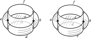
Figure 7: Two isomorphic foams $F_{1}$ (left) and $F_{2}$ (right), corresponding to the bifolds $W_{1}^{\prime}$ and $W_{2}^{\prime}$. Their boundaries are identified with $\Gamma$ in two different ways.

Figure 7, regarded as a foams in $B^{4}$ with boundary $\Gamma$. These two foams are isomorphic, but not by an isomorphism which is the identity on the boundary. Thus, as drawn, $F_{1}$ and $F_{2}$ are the same foam, with two different identifications of the boundary with $\Gamma$. The identifications are indicated by the labeling of the edges in the figure.

Since the smallest action of a moduli space on $Z_{3}$ is $1/32$, the limiting solution on $W^{\prime}_{1}$ or $W^{\prime}_{2}$ in either case must have action $0$, and must therefore be flat. For each of the (isomorphic) bifolds $W^{\prime}_{1}$ and $W^{\prime}_{2}$, there is just one flat bifold connection up to conjugacy.

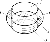
Figure 8: The $V_{4}$-connection for the bifolds $W^{\prime}_{i}$.

This unique connection is a $V_{4}$-connection, in which the links of the faces are mapped to the non-trivial elements $\{i,j,k\}$ of $V_{4}$ as shown in Figure 8. Inspecting Figure 7, we see that, in the case of $W^{\prime}_{1}$, the links of the edges $c$ and $e$ for $\Gamma$ are both mapped to $j$, while for $W^{\prime}_{2}$, one is mapped to $j$ and the other to $k$. That is to say, the unique bifold connection on $W^{\prime}_{1}$ (respectively, $W^{\prime}_{2}$) restricts to the endpoint $0$ (respectively $\pi/2$) in the representation variety $R(S_{2,1})\cong[0,\pi/2]$.

To summarize this, if we divide the ends of $M_{W}$ into two classes, according to which end of $G$ they lie over, then the restriction map $r$ maps the ends of $M_{W}$ belonging to these two classes properly to the two different ends of the interval $(0,\pi/2)$. An analysis of the glueing problem for the connected sum shows that there is just one end in each class. Indeed, the connected sum is the same as the second case of Proposition 4.3, but now the gluing parameter $V$ extends as the group of automorphisms of the bifold connection on $W^{\prime}_{1}$ (or $W^{\prime}_{2}$), so we have just one end instead of two. The proposition follows. ∎

The remainder of the proof that $U_{S_{2,1}}$ is chain-homotopic to the identity follows the argument in [8]; and Theorem 3.1 follows.

8 Deducing the other exact triangles

We have now proved Theorem 3.1, which becomes Theorem 1.1 when applied to webs in $\mathbb{R}^{3}$. We now turn to Theorem 1.2. Because of the cyclic symmetry, it is only necessary to treat one of the three cases, so we take $i=1$. A proof can be constructed by following the same general outline as the previous sections. The composite cobordisms have the same description as shown in Figure 5, except that the disks $\Delta_{0}^{-}$, $\Delta_{2}$ and $\Delta_{3}^{+}$ are absent. The proof proceeds as before, except that the role of $\Psi_{2}$ will now be played by $\Psi_{0}$ and the role of $\Psi_{3}$ by $\Psi_{1}$. We also lose some of the symmetry between the three webs, so the proof needs to treat three cases.

Rather than repeat the details, we give here an alternative argument, showing how to deduce Theorem 1.2 from Theorem 1.1 by applying the basic properties of $J^{\sharp}$ and the results of section 4.

Let $L_{2}$, $L_{1}$ and $L_{0}$ be three webs which again differ only inside a ball, as indicated in (1). Let $\tilde{L}_{i}$ be obtained from $L_{i}$ by attaching an extra edge, as shown in the following diagram:

$$\tilde{L}_{2}={\begin{array}[]{c}\raisebox{-2.5pt}{\includegraphics[width=43.36464pt]{figures/Graph-Xbar-extra}}\end{array}},\qquad\tilde{L}_{1}={\begin{array}[]{c}\raisebox{-2.5pt}{\includegraphics[width=43.36464pt]{figures/Graph-H-extra}}\end{array}},\qquad\tilde{L}_{0}={\begin{array}[]{c}\raisebox{-2.5pt}{\includegraphics[width=43.36464pt]{figures/Graph-I-extra}}\end{array}}.$$ (13)

In each case, the added edge is the top edge in the diagram, which we call $e$, so

$$\tilde{L}_{i}=L_{i}\cup e.$$

We have the standard cobordisms $\Sigma_{i,i-1}$ from $L_{i}$ to $L_{i-1}$ as before, and these give rise to cobordisms

$$\tilde{\Sigma}_{i,i-1}=\Sigma_{i,i-1}\cup[0,1]\times e$$

from $\tilde{L}_{i}$ to $\tilde{L}_{i-1}$.

Theorem 1.1 tells us that we have an exact sequence

$$\cdots\longrightarrow J^{\sharp}(\tilde{L}_{2})\longrightarrow J^{\sharp}(\tilde{L}_{1})\longrightarrow J^{\sharp}(\tilde{L}_{0})\longrightarrow J^{\sharp}(\tilde{L}_{2})\longrightarrow\cdots$$

where the maps are those arising from the cobordisms $\tilde{\Sigma}_{i,i-1}$, or in pictures:

$$\cdots\longrightarrow{\begin{array}[]{c}\raisebox{-2.5pt}{\includegraphics[width=43.36464pt]{figures/Graph-Xbar-extra}}\end{array}}\longrightarrow{\begin{array}[]{c}\raisebox{-2.5pt}{\includegraphics[width=43.36464pt]{figures/Graph-H-extra}}\end{array}}\longrightarrow{\begin{array}[]{c}\raisebox{-2.5pt}{\includegraphics[width=43.36464pt]{figures/Graph-I-extra}}\end{array}}\longrightarrow{\begin{array}[]{c}\raisebox{-2.5pt}{\includegraphics[width=43.36464pt]{figures/Graph-Xbar-extra}}\end{array}}\longrightarrow\cdots$$ (14)

where the application of $J^{\sharp}$ to these terms is implied. If we apply the “triangle relation” [6, Proposition LABEL:prop:triangle-relation] to $\tilde{L}_{0}$ we see that there is an isomorphism on $J^{\sharp}$ between $L_{0}$ and $\tilde{L}_{0}$:

$${\begin{array}[]{c}\raisebox{-2.5pt}{\includegraphics[width=43.36464pt]{figures/Graph-I}}\end{array}}\stackrel{{\scriptstyle\cong}}{{\longrightarrow}}{\begin{array}[]{c}\raisebox{-2.5pt}{\includegraphics[width=43.36464pt]{figures/Graph-I-extra}}\end{array}}.$$

From the square relation [6, Proposition LABEL:prop:square-relation], we obtain isomorphisms

$${\begin{array}[]{c}\raisebox{-2.5pt}{\includegraphics[width=43.36464pt]{figures/Graph-Res1}}\end{array}}\oplus{\begin{array}[]{c}\raisebox{-2.5pt}{\includegraphics[width=43.36464pt]{figures/Graph-Res0}}\end{array}}\stackrel{{\scriptstyle\cong}}{{\longrightarrow}}{\begin{array}[]{c}\raisebox{-2.5pt}{\includegraphics[width=43.36464pt]{figures/Graph-H-extra}}\end{array}}$$ (15)

and

$${\begin{array}[]{c}\raisebox{-2.5pt}{\includegraphics[width=43.36464pt]{figures/Graph-X}}\end{array}}\oplus{\begin{array}[]{c}\raisebox{-2.5pt}{\includegraphics[width=43.36464pt]{figures/Graph-Res0}}\end{array}}\stackrel{{\scriptstyle\cong}}{{\longrightarrow}}{\begin{array}[]{c}\raisebox{-2.5pt}{\includegraphics[width=43.36464pt]{figures/Graph-Xbar-extra}}\end{array}}.$$ (16)

Using these isomorphism to substitute for the terms in the exact sequence (14), we obtain an isomorphic exact sequence

$$\cdots\stackrel{{\scriptstyle\sigma_{2}}}{{\longrightarrow}}\begin{bmatrix}{\begin{array}[]{c}\raisebox{-2.5pt}{\includegraphics[width=34.69038pt]{figures/Graph-X}}\end{array}}\\ \oplus\\ {\begin{array}[]{c}\raisebox{-2.5pt}{\includegraphics[width=34.69038pt]{figures/Graph-Res0}}\end{array}}\end{bmatrix}\stackrel{{\scriptstyle\sigma_{1}}}{{\longrightarrow}}\begin{bmatrix}{\begin{array}[]{c}\raisebox{-2.5pt}{\includegraphics[width=34.69038pt]{figures/Graph-Res1}}\end{array}}\\ \oplus\\ {\begin{array}[]{c}\raisebox{-2.5pt}{\includegraphics[width=34.69038pt]{figures/Graph-Res0}}\end{array}}\end{bmatrix}\stackrel{{\scriptstyle\sigma_{0}}}{{\longrightarrow}}{\begin{array}[]{c}\raisebox{-2.5pt}{\includegraphics[width=34.69038pt]{figures/Graph-I}}\end{array}}\stackrel{{\scriptstyle\sigma_{2}}}{{\longrightarrow}}\begin{bmatrix}{\begin{array}[]{c}\raisebox{-2.5pt}{\includegraphics[width=34.69038pt]{figures/Graph-X}}\end{array}}\\ \oplus\\ {\begin{array}[]{c}\raisebox{-2.5pt}{\includegraphics[width=34.69038pt]{figures/Graph-Res0}}\end{array}}\end{bmatrix}\stackrel{{\scriptstyle\sigma_{1}}}{{\longrightarrow}}\cdots$$ (17)

The maps $\sigma_{i}$ in this sequence are obtained from the foam cobordisms $\tilde{\Sigma}_{i+1,i}$ and the isomorphisms from the triangle and square relations.

The claim in Theorem 1.2 (for $i=0$) is that there is an exact sequence

$$\cdots\stackrel{{\scriptstyle\tau_{2}}}{{\longrightarrow}}{\begin{array}[]{c}\raisebox{-2.5pt}{\includegraphics[width=34.69038pt]{figures/Graph-X}}\end{array}}\stackrel{{\scriptstyle\tau_{1}}}{{\longrightarrow}}{\begin{array}[]{c}\raisebox{-2.5pt}{\includegraphics[width=34.69038pt]{figures/Graph-Res1}}\end{array}}\stackrel{{\scriptstyle\tau_{0}}}{{\longrightarrow}}{\begin{array}[]{c}\raisebox{-2.5pt}{\includegraphics[width=34.69038pt]{figures/Graph-I}}\end{array}}\stackrel{{\scriptstyle\tau_{2}}}{{\longrightarrow}}{\begin{array}[]{c}\raisebox{-2.5pt}{\includegraphics[width=34.69038pt]{figures/Graph-X}}\end{array}}\stackrel{{\scriptstyle\tau_{1}}}{{\longrightarrow}}\cdots$$ (18)

where the maps $\tau_{i}$ arise from the standard cobordisms. The exactness of this sequence will follow if we can show the following relations between the maps:

Proposition 8.1.

The maps $\sigma_{i}$ and $\tau_{i}$ in the above diagrams are related by

$$\sigma_{1}=\begin{bmatrix}\tau_{1}&0\\ 0&1\end{bmatrix},\qquad\sigma_{0}=\begin{bmatrix}\tau_{0}&0\end{bmatrix},\qquad\sigma_{2}=\begin{bmatrix}\tau_{2}\\ 0\end{bmatrix}.$$

For the proof of the proposition, we need the following lemma.

Lemma 8.2.

Let $\Sigma_{2,1}$ be the standard cobordism with a single tetrahedral point,

$${\begin{array}[]{c}\raisebox{-2.5pt}{\includegraphics[width=43.36464pt]{figures/Graph-Xbar}}\end{array}}\stackrel{{\scriptstyle\Sigma_{2,1}}}{{\longrightarrow}}{\begin{array}[]{c}\raisebox{-2.5pt}{\includegraphics[width=43.36464pt]{figures/Graph-H}}\end{array}}.$$

Let $T_{2,1}$ be the standard cobordism from $K_{2}$ to $K_{1}$,

$${\begin{array}[]{c}\raisebox{-2.5pt}{\includegraphics[width=43.36464pt]{figures/Graph-X}}\end{array}}\stackrel{{\scriptstyle T_{2,1}}}{{\longrightarrow}}{\begin{array}[]{c}\raisebox{-2.5pt}{\includegraphics[width=43.36464pt]{figures/Graph-Res1}}\end{array}},$$

and let $\tilde{T}_{2,1}$ be the union of $T_{2,1}$ with a product $[0,1]\times f$, where $f$ is an extra edge:

$${\begin{array}[]{c}\raisebox{-2.5pt}{\includegraphics[width=43.36464pt]{figures/Graph-Xbar-shift}}\end{array}}\stackrel{{\scriptstyle\tilde{T}_{2,1}}}{{\longrightarrow}}{\begin{array}[]{c}\raisebox{-2.5pt}{\includegraphics[width=43.36464pt]{figures/Graph-H-shift}}\end{array}}.$$

Then $\Sigma_{2,1}$ and $\tilde{T}_{2,1}$ give rise to the same map on $J^{\sharp}$.

Proof.

The cobordism $\tilde{T}_{2,1}$ is isomorphic to a connect sum of $\Sigma_{2,1}\#_{t,t_{2}}\Psi_{2}$, where $t$ is the tetrahedral point. The result follows from Proposition 4.3. ∎

Proof of Proposition 8.1.

We illustrate the arguments with one case, showing that the top left entry in the matrix for $\sigma_{1}$ is equal to $\tau_{1}$.

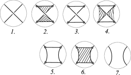
Figure 9: A movie for a foam equivalent to the top-left entry of $\sigma_{1}$.

Consider the foam described by the movie in Figure 9. The first three frames of the movie realize the first component of the isomorphism (16). Frames 3–5 are the addition of a standard $1$-handle, which realize the same map as $\tilde{\Sigma}_{2,1}$, by the lemma above. Frames 5–7 realize the first component of the inverse of the isomorphism (15). Taken together, the foam described by all seven frames gives a map equal to the top-left component of $\sigma_{1}$.

Regard the movie as defining a foam $S$ in the $4$-ball $[1,7]\times B^{3}$. The boundary of this foam is an unknot consisting of the two arcs at $t=1$, the two arcs at $t=7$, and the product $[1,7]\times\{\text{four points on the boundary}\}$. Let $\bar{S}$ be closed foam in $\mathbb{R}^{4}$ obtained by attaching a disk $D$ to this unknot, on the outside of the ball. Then, tautologically,

$$S=T_{2,1}\#\bar{S},$$

where $T_{2,1}$ is the standard $1$-handle cobordism from $K_{2}$ to $K_{1}$, and the connect sum with $\bar{S}$ is made at a point of $D\subset\bar{S}$. The claim is therefore that $T_{2,1}$ and $T_{2,1}\#\bar{S}$ define the same map. An examination of the movie shows that

$$\bar{S}\cong\Psi,$$

where $\Psi$ is the foam that appears in Proposition 4.7, in such a way that the disk $D$ in $\bar{S}$ corresponds to the disk $D^{+}$ in $\Psi$. So the present claim follows from that proposition. ∎

9 The octahedral diagram

We now turn to the diagram in Figure 1, and will verify the properties discussed in the introduction. They are summarized in the following theorem.

Theorem 9.1.

In the diagram of standard cobordisms pictured in Figure 1, the triangles involving

1. $L_{0}$, $K_{2}$, $K_{1}$,

2. $L_{1}$, $K_{0}$, $K_{2}$,

3. $L^{\prime}_{2}$, $K_{0}$, $K_{1}$, and

4. $L^{\prime}_{2}$, $L_{0}$, $L_{1}$

become exact triangles on applying $J^{\sharp}$. The faces

1. $K_{0}$, $K_{2}$, $K_{1}$,

2. $L_{0}$, $K_{2}$, $L_{1}$,

3. $K_{1}$, $L_{2}^{\prime}$, $L_{0}$, and

4. $L_{1}$, $L_{2}^{\prime}$, $K_{0}$

become commutative diagrams. And finally,

1. the composites $K_{2}\to K_{1}\to L_{2}^{\prime}$ and $K_{2}\to L_{1}\to L_{2}^{\prime}$ give the same map on $J^{\sharp}$, and

2. the composites $L^{\prime}_{2}\to K_{0}\to K_{2}$ and $L^{\prime}_{2}\to L_{0}\to K_{2}$ give the same map on $J^{\sharp}$.

Proof.

The first two items are verbatim restatements of cases of Theorem 1.2. The second two cases are cases of Theorem 1.2 and Theorem 1.1. (The pictures are rotated a quarter turn relative to the standard pictures. Alternatively, these pictures portray the dual of the standard triangles.)

The composite cobordism $K_{0}\to K_{2}\to K_{1}$ is equal to the connect sum $\Sigma\#\Psi_{0}$, where $\Sigma$ is the standard cobordism from $K_{0}$ to $K_{1}$ [8]. So the commutativity in case (e) follows from Proposition 4.5. The next three cases of the theorem are similar, except that the connect sums are with $\Psi_{2}$ at a tetrahedral point in case (f), and with $\Psi_{2}$ at a seam point in cases (g) and (h). So Propositions 4.3 and 4.4 deal with these cases.

In each of the final two cases of the theorem, the first composite cobordism is obtained from the second composite by forming a connect sum with $\Psi_{2}$ at a tetrahedral point. So these cases are also consequences of Proposition 4.3. ∎

10 Equivalent formulations of the Tutte relation

The authors conjectured in [6] that if $K$ is a planar web (i.e. is contained in $\mathbb{R}^{2}\subset\mathbb{R}^{3}$), then the dimension of $J^{\sharp}(K)$ is equal to the number of Tait colorings of the underlying abstract graph. (See Conjecture LABEL:thm:Tait-count in [6].) As explained there, confirming this conjecture would provide a new proof of Appel and Haken’s four-color theorem. If we write $\tau(K)$ for the number of Tait colorings of $K$, then $\tau$ is uniquely characterized, for planar webs, by the following properties:

1. $\tau(K)=3$ if $K$ is a circle;

2. $\tau(K)=0$ if $K$ has a bridge;

3. $\tau$ is multiplicative for disjoint unions of planar webs;

4. $\tau$ satisfies the “Tutte relation”, namely if $K_{0}$, $K_{1}$, $L_{0}$, $L_{1}$ are planar webs which differ only in a ball, in the following manner,

   $$K_{0}={\begin{array}[]{c}\raisebox{-2.5pt}{\includegraphics[width=34.2537pt]{figures/Graph-Res0}}\end{array}},\qquad K_{1}={\begin{array}[]{c}\raisebox{-2.5pt}{\includegraphics[width=34.2537pt]{figures/Graph-Res1}}\end{array}},\qquad L_{0}={\begin{array}[]{c}\raisebox{-2.5pt}{\includegraphics[width=34.2537pt]{figures/Graph-I}}\end{array}},\qquad L_{1}={\begin{array}[]{c}\raisebox{-2.5pt}{\includegraphics[width=34.2537pt]{figures/Graph-H}}\end{array}},$$

   then

   $$\tau(K_{0})-\tau(K_{1})+\tau(L_{0})-\tau(L_{1})=0.$$ (19)

The first three of these properties hold also for the quantity $\dim J^{\sharp}(K)$, for planar webs $K$. They are proved in [6]. So the question of whether $\dim J^{\sharp}(K)$ is equal to the number of Tait colorings is equivalent to the following conjecture:

Conjecture 10.1.

If $K_{0}$, $K_{1}$, $L_{0}$, $L_{1}$ are three planar webs differing only in a ball as shown above, then

$$\dim J^{\sharp}(K_{0})-\dim J^{\sharp}(K_{1})+\dim J^{\sharp}(L_{0})-\dim J^{\sharp}(L_{1})=0.$$ (20)

The four webs that appear in this conjecture appear also as the four vertices of the central rectangle in the octahedral diagram, Figure 1. We reproduce that part of the diagram here:

$$\begin{array}[]{c}\includegraphics[scale={0.46}]{figures/Tutte-rectangle}\end{array}$$ (21)

Lemma 10.2.

In the rectangle above, the composite of any two consecutive foams is the zero map on $J^{\sharp}$. So the vector spaces $J^{\sharp}(K_{0})$, $J^{\sharp}(K_{1})$, $J^{\sharp}(L_{0})$, $J^{\sharp}(L_{1})$, together with the maps between them, form a chain complex which is periodic mod $4$.

Proof.

Referring to Figure 1 and Theorem 9.1, we see that (with the application of $J^{\sharp}$ implied), $t\circ\gamma=t\circ b\circ a$, because $\gamma=b\circ a$. On the other hand, $t\circ b=0$, because these are two sides of an exact triangle. This shows that $t\circ\gamma=0$, and essentially the same argument deals with the composites at the other three vertices. ∎

We can now interpret Conjecture 10.1 as asserting that the Euler characteristic of the $4$-periodic complex (21) is zero. Since the Euler characteristic can be computed equally as the alternating sum of the dimensions of the chain groups or as the alternating sum of the dimensions of the homology groups, the left-hand side of (20) can be expressed also as

$$\left|\frac{\ker(\gamma)}{\mathrm{im}(s)}\right|-\left|\frac{\ker(t)}{\mathrm{im}(\gamma)}\right|+\left|\frac{\ker(\xi)}{\mathrm{im}(t)}\right|-\left|\frac{\ker(s)}{\mathrm{im}(\xi)}\right|,$$ (22)

where $|V|$ denotes the dimension of the vector space $V$, and $J^{\sharp}$ is understood.

Lemma 10.3.

In the $4$-periodic complex (21), the homology groups at diametrically opposite corners are equal. Furthermore, the Euler characteristic (22) is equal to

$$2\bigl{(}\mathop{\mathrm{missing}}{rank}(a\circ\kappa)-\mathop{\mathrm{missing}}{rank}(\lambda\circ b)\bigr{)},$$

and also equal to

$$2\bigl{(}\mathop{\mathrm{missing}}{rank}(a)-\mathop{\mathrm{missing}}{rank}(b)\bigr{)}.$$

Here $a$, $b$, $\kappa$ and $\lambda$ are the maps corresponding to the standard cobordisms in Figure 1, and the application of $J^{\sharp}$ is implied.

Proof.

From the exactness of the triangles of maps $(\lambda,\kappa,\gamma)$ and $(a,r,s)$, we have $\ker(\gamma)=\mathrm{im}(\kappa)$ and $\mathrm{im}(s)=\ker(a)$. So

$$\frac{\ker(\gamma)}{\mathrm{im}(s)}=\frac{\mathrm{im}(\kappa)}{\ker(a)}.$$

At the same time, we learn that $\ker(a)\subset\mathrm{im}(\kappa)$, so that the dimension of $\mathrm{im}(\kappa)/\ker(a)$ is equal to the rank of $a\circ\kappa$. Thus

$$\left|\frac{\ker(\gamma)}{\mathrm{im}(s)}\right|=\mathop{\mathrm{missing}}{rank}(a\circ\kappa).$$

A similar discussion can be applied to each of the four terms in (22), so the dimensions of the four quotients that appear there are respectively

$$\mathop{\mathrm{missing}}{rank}(a\circ\kappa),\quad\mathop{\mathrm{missing}}{rank}(\lambda\circ b),\quad\mathop{\mathrm{missing}}{rank}(q\circ\zeta),\quad\mathop{\mathrm{missing}}{rank}(\eta\circ r).$$

The last two parts of Theorem 9.1 say that $\lambda\circ b=\eta\circ r$ and $a\circ\kappa=q\circ\zeta$. So alternate terms of the above four are equal. This verifies the first assertion in the lemma, and also shows that the Euler characteristic is equal to $2(\mathop{\mathrm{missing}}{rank}(a\circ\kappa)-\mathop{\mathrm{missing}}{rank}(\lambda\circ b))$.

From the exact triangle $(a,r,s)$, we have

$$2\mathop{\mathrm{missing}}{rank}(a)=\left|{\begin{array}[]{c}\raisebox{-2.5pt}{\includegraphics[width=34.2537pt]{figures/Graph-Res0}}\end{array}}\right|-\left|{\begin{array}[]{c}\raisebox{-2.5pt}{\includegraphics[width=34.2537pt]{figures/Graph-H}}\end{array}}\right|+\left|{\begin{array}[]{c}\raisebox{-2.5pt}{\includegraphics[width=34.2537pt]{figures/Graph-X}}\end{array}}\right|,$$

while from the exact triangle $(b,t,q)$, we have

$$2\mathop{\mathrm{missing}}{rank}(b)=\left|{\begin{array}[]{c}\raisebox{-2.5pt}{\includegraphics[width=34.2537pt]{figures/Graph-Res1}}\end{array}}\right|-\left|{\begin{array}[]{c}\raisebox{-2.5pt}{\includegraphics[width=34.2537pt]{figures/Graph-I}}\end{array}}\right|+\left|{\begin{array}[]{c}\raisebox{-2.5pt}{\includegraphics[width=34.2537pt]{figures/Graph-X}}\end{array}}\right|.$$

Taking the difference of these last two equalities, we obtain

$$2\mathop{\mathrm{missing}}{rank}(a)-2\mathop{\mathrm{missing}}{rank}(b)=\left|{\begin{array}[]{c}\raisebox{-2.5pt}{\includegraphics[width=34.2537pt]{figures/Graph-Res0}}\end{array}}\right|-\left|{\begin{array}[]{c}\raisebox{-2.5pt}{\includegraphics[width=34.2537pt]{figures/Graph-H}}\end{array}}\right|+\left|{\begin{array}[]{c}\raisebox{-2.5pt}{\includegraphics[width=34.2537pt]{figures/Graph-I}}\end{array}}\right|-\left|{\begin{array}[]{c}\raisebox{-2.5pt}{\includegraphics[width=34.2537pt]{figures/Graph-Res1}}\end{array}}\right|.$$

This is the last assertion of the lemma. ∎

Remarks.

Since Conjecture 10.1 asserts the vanishing of an Euler characteristic for planar webs, it is natural to ask whether something stronger is true, namely that the $4$-periodic sequence of maps (21) is exact. By the proof of the above lemma, this would be equivalent to the vanishing of the composites $a\circ\kappa$ and $\lambda\circ b$. Although this holds in simple cases, it does not appear to be true in general. Calculations for the case that $L_{0}$ is the $1$-skeleton of a dodecahedron (in the natural planar projection) suggest that the rank of $a\circ\kappa$ is $5$ in this case [5]. From this it follows (by the lemma) that the Euler characteristic of the complex is at most $10$. The webs $K_{0}$, $K_{1}$ and $L_{1}$ in this example are “simple webs” in the sense of [6], so $J^{\sharp}$ is easily computed for these three. The inequality on the Euler characteristic then tells us that the dimension of $J^{\sharp}$ of the dodecahedral graph is at most $70$. In the other direction, a different calculation [5] leads to a lower bound of $58$ on the dimension. So we have

$$58\leq\dim J^{\sharp}(\text{Dodecahedron})\leq 70.$$

The number of Tait colorings, on the other hand, is $60$.

A slightly sharper upper bound for the dimension of $J^{\sharp}$ of the dodecahedron arises by a different argument. In [7], the representation variety $\mathcal{R}^{\sharp}(K)$ is described for the dodecahedron: it consists of $10$ copies of the flag manifold and two copies of $\mathop{\mathit{SO}}(3)$. The Chern-Simons functional is Morse-Bott along $\mathcal{R}^{\sharp}(K)$, and it follows that there is a perturbation of the Chern-Simons functional having exactly $68$ critical points, leading to a bound of $68$ on the rank of $J^{\sharp}$. From this point of view, the question of whether the rank is strictly less than $68$ is therefore the question of whether there are any non-trivial differentials in the complex, for this particular perturbation.

References

- [1] M. Abreu. Kähler metrics on toric orbifolds. J. Differential Geom., 58(1):151–187, 2001.
- [2] M. F. Atiyah, N. J. Hitchin, and I. M. Singer. Self-duality in four-dimensional Riemannian geometry. Proc. Roy. Soc. London Ser. A, 362(1711):425–461, 1978.
- [3] R. L. Bryant. Bochner-Kähler metrics. J. Amer. Math. Soc., 14(3):623–715 (electronic), 2001.
- [4] P. Kronheimer, T. Mrowka, P. Ozsváth, and Z. Szabó. Monopoles and lens space surgeries. Ann. of Math. (2), 165(2):457–546, 2007.
- [5] P. B. Kronheimer and T. S. Mrowka. Foam calculations for the instanton homology of the dodecahedron. In preparation.
- [6] P. B. Kronheimer and T. S. Mrowka. Tait colorings, and an instanton homology for webs and foams. Preprint, 2015.
- [7] P. B. Kronheimer and T. S. Mrowka. The representation variety for the dodecahedral web. In preparation.
- [8] P. B. Kronheimer and T. S. Mrowka. Khovanov homology is an unknot-detector. Publ. Math. IHES, 113:97–208, 2012.
- [9] P. Ozsváth and Z. Szabó. On the Heegaard Floer homology of branched double-covers. Adv. Math., 194(1):1–33, 2005.