TTP15-033

Charge and color breaking constraints in the Minimal Supersymmetric Standard Model associated with the bottom Yukawa coupling

Wolfgang Gregor Hollik

Institut für Theoretische Teilchenphysik, Karlsruhe Institute of Technology

Engesserstraße 7, D-76131 Karlsruhe, Germany

Testing the stability of the electroweak vacuum in any extension of the Standard Model Higgs sector is of great importance to verify the consistency of the theory. Multi-scalar extensions as the Minimal Supersymmetric Standard Model generically lead to unstable configurations in certain regions of parameter space. An exact minimization of the scalar potential is rather an impossible analytic task. To give handy analytic constraints, a specific direction in field space has to be considered which is a simplification that tends to miss excluded regions, however good to quickly check parameter points. We describe a yet undescribed class of charge and color breaking minima as they appear in the Minimal Supersymmetric Standard Model, exemplarily for the case of non-vanishing bottom squark vacuum expectation values constraining the combination $\mu Y_{\mathrm{b}}$ in a non-trivial way. Contrary to famous $A$-parameter bounds, we relate the bottom Yukawa coupling with the supersymmetry breaking masses. Another bound can be found relating soft breaking masses and $\mu$ only. The exclusions follow from the tree-level minimization and can change dramatically using the one-loop potential. Estimates of the lifetime of unstable configurations show that they are either extremely short- or long-lived.

Keywords: Minimal Supersymmetric Standard Model, charge and color breaking minima, vacuum stability
PACS: 11.15.Ex, 11.30.Pb, 12.60.Jv

1 Introduction

A complete analysis of the vacuum structure in any quantum field theory needs a consideration of the effective potential to all orders which is more than an honorable task. Important contributions to the effective potential in the Standard Model and supersymmetrized versions at one and way more loops have been (partially) determined [1, 2, 3, 4, 5, 6]. The more loops the more difficult is also the task to find the global minimum which shall determine the vacuum state of the theory. Numerical solutions to that problem exist in the Minimal Supersymmetric Standard Model (MSSM) where both the effective potential as well as the (expected-to-be) global minimum are calculated and determined purely numerically [7, 8]. Supersymmetry (SUSY) generically tends to stabilize the potential as negative fermionic loop contributions are compensated by the corresponding bosonic ones. The superpartner spectrum on the other hand brings additional directions in scalar field space that potentially invalidate the electroweak Higgs vacuum at the classical level. A physical viable supersymmetric extension has to take care of the additional parameters in a way that the “desired” vacuum is the true vacuum of the theory.

The consideration of the one-loop effective potential, which can be very efficiently done via the famous formula of Coleman and Weinberg [1], leads to a first understanding of non-trivial minima. We have

$$V_{\text{CW}}=\frac{1}{64\pi^{2}}\sum_{f}C_{f}\operatorname{STr}\left[\mathcal{M}_{f}^{4}(\phi)\left(\ln\big{(}\mathcal{M}_{f}^{2}(\phi)/Q^{2}\big{)}+P_{f}(\phi)\right)\right],$$ (1)

where the sum runs over all fields $f$ in the loop and $C_{f}$ counts gauge degrees of freedom like $C_{\text{quark}}=3$ (spin degrees of freedom are covered by the supertrace $\operatorname{STr}$). The field-dependent mass eigenvalues $\mathcal{M}_{f}(\phi)$ are generically the eigenvalues of the Hessian matrix of the full scalar potential and the field $\phi$ represents any type of scalar field value which is still present in the masses (do not set remnant field values to zero, they correspond to vacuum expectation values (vevs) at local or global minima of the potential). Additionally, there is a polynomial $P_{f}(\phi)$ which is renormalization scheme dependent and in the most common cases a constant. The renormalization scale is given by $Q$.

The one-loop potential is known to develop an imaginary part [9, 10, 8, 11] which is of no importance in the discussion of tunneling times from false to true vacua but opens the access to non-standard vacua: an imaginary part in the one-loop effective potential is related to a non-convex tree-level potential at that point. A non-convex potential means that the second derivative is negative which corresponds to a tachyonic mass eigenvalue $\mathcal{M}_{f}^{2}(\phi)<0$. The tachyonic mass, however, would only be present at the minimum (which by definition is locally convex). So, the existence of a non-convex direction points towards a minimum in that direction unless the potential is unbounded from below, which would be even worse. Finding the critical field value at which the non-convex direction opens is trivial as we shall see. The question is rather whether the non-standard minimum is deeper than the standard one and therefore allows for a vacuum-to-vacuum transition which can be figured out analytically under certain circumstances.

We first consider the loop corrected Higgs potential in the MSSM including SUSY loop contributions from the third generation (s)fermions. The tree-level part is given by the mass terms and the self-couplings which are gauge couplings. The one-loop part is given by the logarithms of Eq. (1) which also follow from the direct calculation [11]. We borrow the notation from [11] and define the effective potential as

$$V_{\text{eff}}= V_{0}+V_{1}^{\tilde{t}}+V_{1}^{t}+V_{1}^{\tilde{b}}+V_{1}^{b}$$ (2)

$$= m_{11}^{2\,^{\text{tree}}}\;|h_{\mathrm{d}}^{0}|^{2}+m_{22}^{2\,^{\text{tree}}}\;|h_{\mathrm{u}}^{0}|^{2}-2\operatorname{Re}\left(m_{12}^{2\,^{\text{tree}}}\;h_{\mathrm{u}}^{0}h_{\mathrm{d}}^{0}\right)+\frac{g_{1}^{2}+g_{2}^{2}}{8}\left(|h_{\mathrm{d}}^{0}|^{2}-|h_{\mathrm{u}}^{0}|^{2}\right)^{2}$$

$$+\frac{N_{c}{\widetilde{M}}_{\mathrm{t}}^{4}}{32\pi^{2}}\bigg{[}\left(1+x_{\mathrm{t}}+y_{\mathrm{t}}\right)^{2}\ln\left(1+x_{\mathrm{t}}+y_{\mathrm{t}}\right)+\left(1-x_{\mathrm{t}}+y_{\mathrm{t}}\right)^{2}\ln\left(1-x_{\mathrm{t}}+y_{\mathrm{t}}\right)$$

$$\qquad\qquad\;-\left(x_{\mathrm{t}}^{2}+2y_{\mathrm{t}}\right)\left(3-2\ln\left({\widetilde{M}}_{\mathrm{t}}^{2}/Q^{2}\right)\right)-2{y_{\mathrm{t}}^{2}}\ln\left(y_{\mathrm{t}}\right)\;+\;\{\mathrm{t}\leftrightarrow\mathrm{b}\}\bigg{]},$$

where the abbreviations $x_{\mathrm{t},\mathrm{b}}$ and $y_{\mathrm{t},\mathrm{b}}$ are

$$x_{\mathrm{t}}^{2} =\frac{\left|A_{\mathrm{t}}h_{\mathrm{u}}^{0}-\mu^{*}Y_{\mathrm{t}}h_{\mathrm{d}}^{0*}\right|^{2}}{{\widetilde{M}}^{4}_{\mathrm{t}}}+\frac{\left({\tilde{m}}^{2}_{Q}-{\tilde{m}}^{2}_{t}\right)^{2}}{4{\widetilde{M}}^{4}_{\mathrm{t}}},\quad y_{\mathrm{t}}=\frac{\left|Y_{\mathrm{t}}h_{\mathrm{u}}^{0}\right|^{2}}{{\widetilde{M}}_{\mathrm{t}}^{2}},$$ (3a)

$$x_{\mathrm{b}}^{2} =\frac{\left|A_{\mathrm{b}}h_{\mathrm{d}}^{0}-\mu^{*}Y_{\mathrm{b}}h_{\mathrm{u}}^{0*}\right|^{2}}{{\widetilde{M}}_{\mathrm{b}}^{4}}+\frac{\left({\tilde{m}}^{2}_{Q}-{\tilde{m}}^{2}_{b}\right)^{2}}{4{\widetilde{M}}^{4}_{\mathrm{b}}},\quad y_{\mathrm{b}}=\frac{\left|Y_{\mathrm{b}}h_{\mathrm{d}}^{0}\right|^{2}}{{\widetilde{M}}_{\mathrm{b}}^{2}}.$$ (3b)

The soft SUSY breaking masses enter as $\tilde{m}_{Q}^{2}$, $\tilde{m}_{t}^{2}$ and $\tilde{m}_{b}^{2}$ and we defined $\widetilde{M}_{\mathrm{t},\mathrm{b}}^{2}=(\tilde{m}_{Q}^{2}+\tilde{m}_{t,b}^{2})/2$. The trilinear soft breaking couplings in the up and down sector are given by $A_{\mathrm{t}}$ and $A_{\mathrm{b}}$, respectively. Yukawa couplings are denoted as $Y_{\mathrm{t},\mathrm{b}}$ and $\mu$ is the $\mu$ parameter of the superpotential in the MSSM. The mass parameters of the tree-level Higgs potential are $m_{11}^{2\,^{\text{tree}}}=m_{H_{\mathrm{d}}}^{2}+|\mu|^{2}$, $m_{22}^{2\,^{\text{tree}}}=m_{H_{\mathrm{u}}}^{2}+|\mu|^{2}$ and $m_{12}^{2\,^{\text{tree}}}=B_{\mu}$ with the soft breaking masses $m_{H_{\mathrm{u}}}^{2}$ and $m_{H_{\mathrm{d}}}^{2}$ for the $H_{\mathrm{u}}$ and $H_{\mathrm{d}}$ doublet, respectively; $B_{\mu}$ is the soft breaking bilinear term $\sim H_{\mathrm{u}}\cdot H_{\mathrm{d}}$. We consider only third generation superfields which couple with large Yukawa couplings to the Higgs doublets:

$$\mathcal{W}=\mu\;H_{\mathrm{d}}\cdot H_{\mathrm{u}}+Y_{\mathrm{t}}\;H_{\mathrm{u}}\cdot Q_{\mathrm{L}}\bar{T}_{\mathrm{R}}-Y_{\mathrm{b}}\;H_{\mathrm{d}}\cdot Q_{\mathrm{L}}\bar{B}_{\mathrm{R}}.$$ (4)

The left-handed doublet field is $Q_{\mathrm{L}}=(T_{\mathrm{L}},B_{\mathrm{L}})$ and the two Higgs doublets $H_{\mathrm{u}}=(h_{\mathrm{u}}^{+},h_{\mathrm{u}}^{0})$ and $H_{\mathrm{d}}=(h_{\mathrm{d}}^{0},-h_{\mathrm{d}}^{-})$; $\mathrm{SU}(2)_{\mathrm{L}}$-invariant multiplication is denoted by the dot-product. The $\mathrm{SU}(2)_{\mathrm{L}}$ singlets are put into the left-chiral supermultiplets $\bar{T}_{\mathrm{R}}=\{\tilde{t}_{\mathrm{R}}^{*},t^{c}_{\mathrm{R}}\}$ and $\bar{B}_{\mathrm{R}}=\{\tilde{b}_{\mathrm{R}}^{*},b_{\mathrm{R}}^{c}\}$ with the charge conjugated Weyl spinors $t^{c}_{\mathrm{R}}$ and $b_{\mathrm{R}}^{c}$.

The effective potential of Eq. (2) obviously develops an imaginary part beyond the branch point of the logarithms $\ln(1\pm x+y)$. We want to give a physical meaning of this branch point without reference to an imaginary part of the effective potential, since $\frac{1}{2}\ln\big{(}(1\pm x+y)^{2}\big{)}$ does not reveal any imaginary part—nevertheless, this logarithm gets singular where $\mp x-y=1$ though the potential itself stays finite. This point determines (for fixed parameters) a critical Higgs field value for which one mass eigenvalue gets tachyonic. The effective potential is a function of the (classical) field values which correspond to vacuum expectation values at the minimum. In the direction of the negative mass square, the potential drops down and therefore develops a CCB vacuum.

Moreover, for certain parameters, the potential of Eq. (2) develops a second minimum in the direction of a standard Higgs vev which always lies beyond the branch point of one of the logarithms [11]. Expanding around this second minimum, one finds exactly one negative sbottom mass square (in the region of large $\mu$ and $\tan\beta$) which hints towards a global minimum including a sbottom vev. The second minimum as depicted in [11] is an artifact of holding $\tilde{b}_{\mathrm{L},\mathrm{R}}=0$: the global minimum lies at a point with both $\langle\tilde{b}_{\mathrm{L},\mathrm{R}}\rangle\neq 0$ and $\langle h_{\mathrm{u}}^{0}\rangle\neq v_{\mathrm{u}}$.

We take the existence of the critical field value serious and first figure out its meaning for the development of such a CCB minimum. For simplification we now restrict ourselves in the following to $\langle\tilde{t}_{L}\rangle=\langle\tilde{t}_{R}\rangle=0$ and also do not consider stau vevs. Let us consider for the moment a fixed value of the down-type Higgs field, $h_{\mathrm{d}}^{0}=v_{\mathrm{d}}$ and set $A_{\mathrm{b}}=0$. The critical field value is then obtained by solving $x_{\mathrm{b}}-y_{\mathrm{b}}=1$ with $x_{\mathrm{b}}$ and $y_{\mathrm{b}}$ given in Eq. (3):

$$h^{0}_{\mathrm{u}}\big{|}_{\text{crit}}=\pm\frac{Y_{\mathrm{b}}^{2}v_{\mathrm{d}}^{2}+M_{\text{SUSY}}^{2}}{\mu Y_{\mathrm{b}}},$$ (5)

with $\tilde{m}_{Q}^{2}=\tilde{m}_{b}^{2}=M_{\text{SUSY}}^{2}$ and $\mu$, $Y_{\mathrm{b}}$ as well as the Higgs field assumed to be real. The bottom Yukawa coupling suffers from SUSY threshold corrections and reads $Y_{\mathrm{b}}=m_{\mathrm{b}}/[v_{\mathrm{d}}(1+\Delta_{b})]$ with $\Delta_{b}$ including the Higgsino corrections $\sim\mu A_{\mathrm{t}}\tan\beta$ [12, 13, 14, 15], which can be dominant over the gluino-induced threshold correction for large $\mu\tan\beta$ and large gluino mass. Both gluino and higgsino contributions sum up together, $\Delta_{b}=\Delta_{b}^{\text{gluino}}+\Delta_{b}^{\text{higgsino}}$, where the interesting one-loop contribution is given by [12, 13, 14, 15]

$$\Delta_{b}^{\text{gluino}} =\frac{2\alpha_{s}}{3\pi}\mu M_{\tilde{G}}\tan\beta I(\tilde{m}_{\tilde{b}_{1}},\tilde{m}_{\tilde{b}_{2}},M_{\tilde{G}}),$$ (6a)

$$\Delta_{b}^{\text{higgsino}} =\frac{Y_{\mathrm{t}}^{2}}{16\pi^{2}}\mu A_{\mathrm{t}}\tan\beta I(\tilde{m}_{\tilde{t}_{1}},\tilde{m}_{\tilde{t}_{2}},\mu),$$ (6b)

with

$$I(m_{1},m_{2},m_{3})=\frac{m_{1}^{2}m_{2}^{2}\ln\frac{m_{2}^{2}}{m_{1}^{2}}+m_{2}^{2}m_{3}^{2}\ln\frac{m_{3}^{2}}{m_{2}^{2}}+m_{1}^{2}m_{3}^{2}\ln\frac{m_{1}^{2}}{m_{3}^{2}}}{(m_{1}^{2}-m_{2}^{2})(m_{1}^{2}-m_{3}^{2})(m_{2}^{2}-m_{3}^{2})}.$$

There are also higher order calculations of $\Delta_{b}$ available that are important for precision analyses [16, 17, 18].

The gluino loop contribution (6a) decouples with the gluino mass if the other SUSY parameters are fixed, but the higgsino one (6b) cannot be neglected for the desired values of $\mu$ around the SUSY scale. For the numerical analysis in the course of this letter, we set $M_{\tilde{G}}=M_{\text{SUSY}}$ which reduces $Y_{\mathrm{b}}$ for positive $\mu$. Moreover, we only include “active” third generation squarks as superpartners and implicitly take any other superpartner heavy (all gauginos besides the gluino which does not give a contribution to the effective Higgs potential at one-loop).

There are handy exclusion limits, well-known for a long time, to simply check whether an unwanted, charge and color breaking (CCB) minimum appears for a given set of parameters in the MSSM. The constraints are on soft breaking trilinear couplings against soft breaking mass parameters as

$$A_{\mathrm{t}}^{2}<3(m_{22}^{2}+{\tilde{m}}_{Q}^{2}+{\tilde{m}}_{t}^{2}),$$ (7)

see e. g. [19, 20, 21, 22, 23, 24, 25, 26].

Mostly studied, however, are such couplings of up-type squarks to the up-type Higgs or of down-type sleptons to the down-type Higgs (where similar expression for down-type squarks can be obtained by relabeling the parameters). Couplings to the “wrong” Higgs doublet are mainly excluded in the analyses. The destabilizing contribution is always related to the trilinear part of the scalar potential, e. g. $\sim\mu Y^{*}_{\mathrm{b}}h_{\mathrm{u}}^{0}\tilde{b}^{*}_{\mathrm{R}}\tilde{b}_{\mathrm{L}}$. It has been shown [11] that the direction of the up-type Higgs field gets apparently destabilized from a (s)bottom loop effect. In [11] only the field direction of the neutral Higgs, $h_{\mathrm{u}}^{0}$, was considered—we now want to give a more complete view of the destabilizing effect leading to an analytic approximate exclusion on the combination $\mu Y_{\mathrm{b}}$ in case the colored sbottom direction is included. Another exclusion can be obtained using a different direction in field space, where also the down-type Higgs scalar is needed.

In this letter, we describe in the following section how to derive the analytic expression for the new CCB constraint from sbottom vevs and compare it to the numerical analysis of the global minima in the quantum (e. g. loop corrected) theory. Finally, we conclude.

2 Finding CCB minima

So far, we only discussed features of the scalar (one-loop) Higgs potential from Eq. (2) as described in [11]. In order to find the new (true) CCB vacuum, which hides behind the critical Higgs field value, we add to the potential of Eq. (2) (evaluated at $Q^{2}=M_{\text{SUSY}}^{2}$) the tree-level part of the sbottom potential,

$$V^{\mathrm{tree}}_{\tilde{b}} =\tilde{b}_{\mathrm{L}}^{*}({\tilde{m}}_{Q}^{2}+|Y_{\mathrm{b}}h^{0}_{\mathrm{d}}|^{2})\tilde{b}_{\mathrm{L}}+\tilde{b}_{\mathrm{R}}^{*}({\tilde{m}}_{b}^{2}+|Y_{\mathrm{b}}h^{0}_{\mathrm{d}}|^{2})\tilde{b}_{\mathrm{R}}$$ (8)

$$\quad-\left[\tilde{b}_{\mathrm{L}}^{*}(\mu^{*}Y_{\mathrm{b}}h_{\mathrm{u}}^{0{\dagger}}-A_{\mathrm{b}}h^{0}_{\mathrm{d}})\tilde{b}_{\mathrm{R}}+\text{h.\,c.\ }\right]+|Y_{\mathrm{b}}|^{2}|\tilde{b}_{\mathrm{L}}|^{2}|\tilde{b}_{\mathrm{R}}|^{2}+\;D\text{-terms}.$$

As was already pointed out before [27, 28], the destabilizing term is always the trilinear one, $\mu Y_{\mathrm{b}}^{*}h_{\mathrm{u}}^{0}\tilde{b}^{*}_{\mathrm{R}}\tilde{b}_{\mathrm{L}}$, so we expect a new stability condition for the combination $\mu Y_{\mathrm{b}}$ taking $A_{\mathrm{b}}=0$. Actually, we cannot ignore $D$-terms in the tree-level potential accordingly to the neglect of all $g_{1,2}^{2}$ terms in the derivation of the one-loop Higgs potential, since also the Higgs self-couplings are $\sim g_{1,2}^{2}$. However, we can simplify (as usually done) the discussion considering so-called “$D$-flat” directions. Those directions are most probably that kind of rays in field space in which unwanted minima develop. Non-$D$-flat directions are protected by the quartic terms that will always take over. The full $D$-term potential for the Higgs and sbottom scalar potential is given by

$$V_{D}= \;\frac{g_{1}^{2}}{8}\big{(}|h_{\mathrm{u}}^{0}|^{2}-|h_{\mathrm{d}}^{0}|^{2}+\frac{1}{3}|\tilde{b}_{L}|^{2}+\frac{2}{3}|\tilde{b}_{R}|^{2}\big{)}^{2}$$ (9)

$$+ \;\frac{g_{2}^{2}}{8}\big{(}|h_{\mathrm{u}}^{0}|^{2}-|h_{\mathrm{d}}^{0}|^{2}+|\tilde{b}_{L}|^{2}\big{)}^{2}+\frac{g_{3}^{2}}{6}\big{(}|\tilde{b}_{L}|^{2}-|\tilde{b}_{R}|^{2}\big{)}^{2}.$$

We still ignore stop and stau fields and remark that the pure Higgs terms are already included in Eq. (2). Nevertheless, we make use of Eq. (9) to set the interesting directions: with $\tilde{b}_{L}=\tilde{b}_{R}\equiv\tilde{b}$, we have the $\mathrm{SU}(3)_{c}$ $D$-flat direction. Considering the three-field scenario, we can reduce the degrees of freedom forcing all $D$-terms to vanish by the choice $|h_{\mathrm{d}}^{0}|^{2}=|h_{\mathrm{u}}^{0}|^{2}+|\tilde{b}|^{2}$. Still rather large quartic terms survive in the potential, namely the $|Y_{\mathrm{b}}|^{2}$ terms from the $F$-term part in $V_{\tilde{b}}^{\text{tree}}$. For that observation, we also look into a non-$D$-flat direction keeping $\frac{g_{1}^{2}+g_{2}^{2}}{8}\big{(}|h_{\mathrm{u}}^{0}|^{2}+|\tilde{b}|^{2}\big{)}^{2}$, where the down-type Higgs is fixed at $h_{\mathrm{d}}^{0}=v_{\mathrm{d}}$ which is a constant and small number especially for large $\tan\beta$, and therefore neglected with respect to potentially large field values of $\tilde{b}$ and $h_{\mathrm{u}}^{0}$. Note that contrary to most previous considerations [27, 26, 29, 30] we are explicitly interested in $\tilde{b}\neq 0$ though $A_{\mathrm{b}}=0$ and have $\tilde{t}_{\mathrm{L},\mathrm{R}}=0$. In both ways we are considering a combined non-standard vacuum in the mixed sbottom and up-type Higgs direction instead of the pure down-down case.

Let us figure out the analytic bound analogously to the famous $A$-parameter bounds like Uneq. (7), under which circumstances a CCB true vacuum appears. For that purpose, we shall choose the most probable field configuration that makes all the $D$-terms vanish. In the $\mathrm{SU}(3)_{c}\times\mathrm{SU}(2)_{\mathrm{L}}\times\mathrm{U}(1)_{Y}$ $D$-flat direction, we assign $\tilde{b}_{\mathrm{L}}=\tilde{b}_{\mathrm{R}}=\tilde{b}$ and ${h^{0}_{\mathrm{d}}}^{2}={h_{\mathrm{u}}^{0}}^{2}+\tilde{b}^{2}$. We consider only real fields and parameters now and in the following for simplicity. A different but not uninteresting bound will be derived in a direction where we keep the $h_{\mathrm{d}}$ field strength at a fixed and small value, $h_{\mathrm{d}}^{0}=v_{\mathrm{d}}\approx 0$. That way, we cannot reduce the quartic terms but still find a (new) analytic exclusion in the $h_{\mathrm{u}}^{0}=\tilde{b}$ direction.

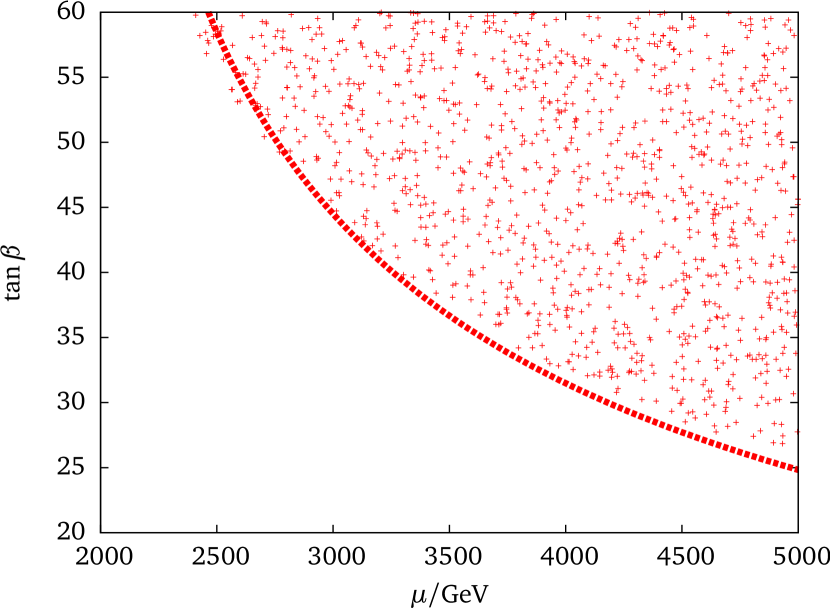
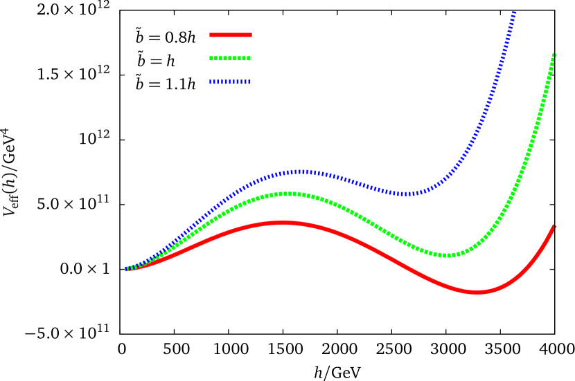
Figure 1: New exclusion limits including the formation of charge and color breaking minima with both $\langle\tilde{b}\rangle\neq 0$ and $\langle h_{\mathrm{u}}^{0}\rangle\neq 0$. The left plot shows exclusions in the $\mu$-$\tan\beta$ plane with $A_{\mathrm{t}}=-1800\,\mathrm{GeV}$ which has been chosen conveniently to give the proper light Higgs mass within a few $\mathrm{GeV}$ and a common soft breaking mass $M_{\text{SUSY}}=1\,\mathrm{TeV}$. The small points are excluded by the numerical comparison of the two minima (exclusion if CCB minimum deeper than trivial one). On the right-hand side we depict the crucial dependence of the non-standard minimum on the (mis)alignment of sbottom field and Higgs field value ($\tilde{b}=\alpha h$ with $h=h_{\mathrm{u}}^{0}$, $h_{\mathrm{d}}^{0}=0$ and $\alpha\in\{0.8,1,1.1\}$ for a given excluded point.

 

$h_{\mathrm{u}}^{0}=\tilde{b}$

An exact analytic derivation of the exclusion limits from the stability of the electroweak vacuum against formation of charge and color breaking minima is very easy to obtain in the one-field scenario. We follow the standard procedure which was pictorially reviewed in Ref. [8]. We collect the interesting parts of the tree-level potentials of Eqs. (2) and (8),

$$V_{\tilde{b},h}^{\text{tree}}=(M^{2}-2\mu Y_{\mathrm{b}}h)\tilde{b}^{2}+m^{2}h^{2}+\lambda_{b}\tilde{b}^{4}+\lambda_{h}h^{4}+\lambda_{hb}h^{2}\tilde{b}^{2},$$ (10)

with $M^{2}={\tilde{m}}_{Q}^{2}+{\tilde{m}}_{b}^{2}$, $m^{2}=m_{H_{\mathrm{u}}}^{2}+\mu^{2}$ and the self-couplings $\lambda_{b}=Y_{\mathrm{b}}^{2}+\frac{g_{1}^{2}+g_{2}^{2}}{8}$, $\lambda_{h}=\frac{g_{1}^{2}+g_{2}^{2}}{8}$ and $\lambda_{hb}=\frac{g_{1}^{2}+g_{2}^{2}}{4}$. This simplifies via $\tilde{b}=h$ further to

$$V_{h,h}^{\text{tree}}=\bar{m}^{2}h^{2}-Ah^{3}+\lambda h^{4},$$ (11)

with $\bar{m}^{2}=M^{2}+m^{2}$, $\lambda=\lambda_{h}+\lambda_{b}+\lambda_{hb}$ and $A=2\mu Y_{\mathrm{b}}$. We then find with the vev,

$$v=\langle h\rangle=\frac{3A+\sqrt{9A^{2}-32\bar{m}^{2}\lambda}}{8\lambda},$$

and the requirement that for stable configurations $V_{\text{min}}=V_{h,h}^{\text{tree}}(v)>0$, which is $\bar{m}^{2}>\frac{A^{2}}{4\lambda}$, the new condition as ($m_{H_{\mathrm{u}}}^{2}$ is negative!)

$$m_{H_{\mathrm{u}}}^{2}+\mu^{2}+{\tilde{m}}_{Q}^{2}+{\tilde{m}}_{b}^{2}>\frac{(\mu Y_{\mathrm{b}})^{2}}{Y_{\mathrm{b}}^{2}+(g_{1}^{2}+g_{2}^{2})/2}.$$ (12)

Note that $Y_{\mathrm{b}}$ has a non-trivial dependence on $\mu$, $\tan\beta$ and also $A_{\mathrm{t}}$ via $\Delta_{b}$, see Eqs. (6) and [12, 13, 14, 15]. The $(g_{1}^{2}+g_{2}^{2})/2$ contribution is the left-over from the non-$D$-flatness which can be numerically of the same size as a threshold-resummed $Y_{\mathrm{b}}$, weakening the exclusion. This bound, however, does not fit exactly to the numerical exclusion as can be seen from Fig. 1 but provides an excellent approximation though actually $\langle h\rangle\neq\langle\tilde{b}\rangle$. The numerical exclusion limit shown in Fig. 1 agrees well with independent previous analyses on a similar situation [31] and are a bit stricter than the final results of [11], whereas a similar necessary condition was found for a slightly different direction in field space [32].

$|h^{0}_{\mathrm{d}}|^{2}=|h_{\mathrm{u}}^{0}|^{2}+|\tilde{b}|^{2}$

With the knowledge from above, it is straightforward to give a similar exclusion in the $D$-flat direction $|h^{0}_{\mathrm{d}}|^{2}=|h_{\mathrm{u}}^{0}|^{2}+|\tilde{b}|^{2}$. The remaining two-field scalar potential (real fields and parameters, $A_{\mathrm{b}}=0$) can be further reduced aligning $\tilde{b}=\alpha h_{\mathrm{u}}^{0}=\alpha h$ with a (real) scaling parameter $\alpha$:

$$V_{D\text{-flat}} =\left(m_{11}^{2}(1+\alpha^{2})+m_{22}^{2}\pm 2m_{12}^{2}\sqrt{1+\alpha^{2}}+\alpha^{2}({\tilde{m}_{Q}}^{2}+{\tilde{m}_{b}}^{2})\right)h^{2}$$ (13)

$$\;-2\mu Y_{\mathrm{b}}\alpha^{2}h^{3}+Y_{\mathrm{b}}^{2}\big{(}2\alpha^{2}(1+\alpha^{2})+\alpha^{4}\big{)}h^{4},$$

that can be easily mapped on the expression of Eq. (11) resulting in the requirement that for stable configurations

$$m_{11}^{2}(1+\alpha^{2})+m_{22}^{2}\pm 2m_{12}^{2}\sqrt{1+\alpha^{2}}+\alpha^{2}({\tilde{m}_{Q}}^{2}+{\tilde{m}_{b}}^{2})>\frac{\mu^{2}\alpha^{2}}{2+3\alpha^{2}}.$$ (14)

This exclusion translated into the $\mu$-$\tan\beta$ plane is shown in Fig. 2 where we also display points that are excluded via the numerical minimization of the combined tree and one-loop effective potential. To enhance the significance of this bound (which is basically $\tan\beta$-independent), we have employed running squark parameters in the tree-level sbottom potential evaluated at the scale of the new minimum. Therefore, also corresponding parameters in the analytic exclusion (soft SUSY breaking masses and $\mu$) have been taken at the same scale. Unfortunately, for the purpose of displaying the exclusion line, it is not clear at which scale those parameters have to be evaluated. As the second minimum generically appears around one order of magnitude above the SUSY scale, we have set a fixed renormalization scale of $10\,M_{\text{SUSY}}$ and therefore blue dots and the reddish area on the left-hand side Fig. 2 do not perfectly fit. Moreover, the excluded area by Uneq. (14) is not completely filled with excluded blue points as there the sbottom-tree plus Higgs-one-loop potential shows a different behavior than the classical potential as also depicted in Fig. 3.

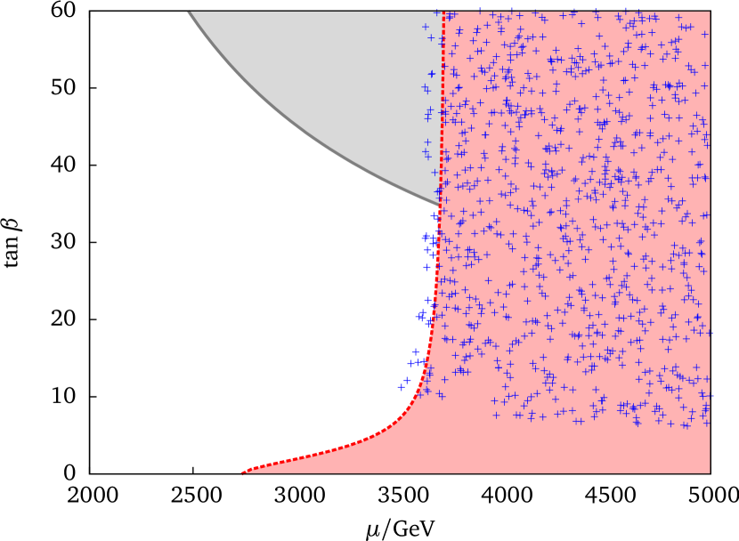
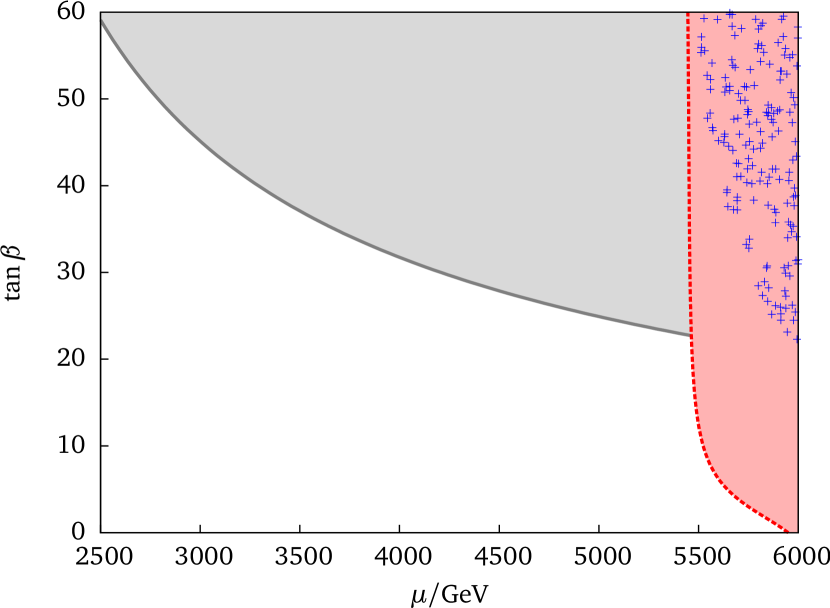
Figure 2: Exclusion in the $\mu$-$\tan\beta$ plane similar to the one shown in Fig. 1 (which is indicated by the grayish area) for the $D$-flat direction $|h_{\mathrm{d}}^{0}|^{2}=|h_{\mathrm{u}}^{0}|^{2}+|\tilde{b}|^{2}$. Blue dots have been excluded via numerical comparison of the two minima (if so) using the one-loop Higgs potential and an improved sbottom potential at the tree-level; the red line shows the exclusion of Uneq. (14) where the misalignment parameter $\alpha$ has been “fitted” for optical agreement of the blue dots and the reddish area to be $0.75$; the actual $\alpha$ are different for each blue point. On the left-hand side, we have the $-$-sign and on the right-hand side the $+$-sign of Uneq. (14).

 

Unequations like (14) or (12) follow from the tree-level potential and can be determined easily once a specific field line is selected. Going beyond tree-level changes the situation severely as can be seen from Fig. 3. A configuration which is obviously unstable ( right-hand side) at the tree-level not even develops a second minimum considering the one-loop Higgs potential (the complete one-loop potential including sbottom directions was not employed for that purpose though should be available numerically). However, this effect is different in the “positive” $h_{\mathrm{d}}^{0}$ direction where unstable configurations are driven towards more stable ones as can be seen from the left-hand side of Fig. 3. Usage of the renormalization group improved (tree-level) effective potential, where the couplings (Yukawa couplings and masses, actually no gauge couplings are they are absent in the genuine $D$-flat direction) are evaluated at a proper scale, hint towards less restrictive exclusions. Where the tree-only potentials show non-trivial charge and color breaking minima, the loop-corrected potentials seem to stabilize the standard vacuum against formation of false vacua.

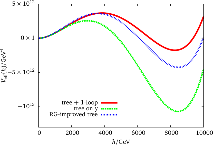
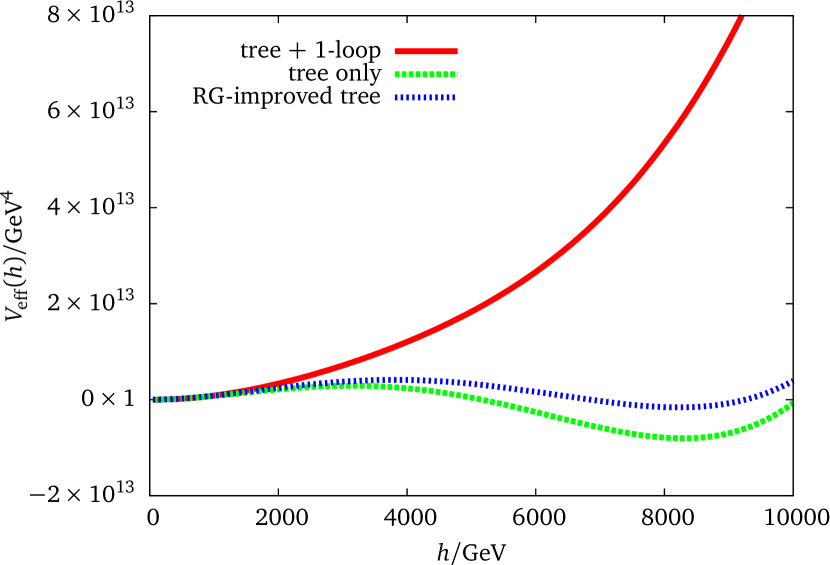
Figure 3: For a given parameter point ($\mu=4\,\mathrm{TeV}$, $\tan\beta=40$, $A_{\mathrm{t}}=1.8\,\mathrm{TeV}$), we show exemplarily the behavior of the potential in the given direction in field space (and $\tilde{b}=0.75h_{\mathrm{u}}^{0}$). On the left-hand side, the positive sign for $h_{\mathrm{d}}^{0}$ was chosen, where the plot on the right has $h_{\mathrm{d}}^{0}=-\sqrt{|h_{\mathrm{u}}^{0}|^{2}+|\tilde{b}|^{2}}$ with real fields and parameters in both cases. The “tree + 1-loop” line means inclusion of the one-loop Higgs potential as of Eq. (2) plus the tree-level bottom squark potential (without $D$-terms each since they vanish by definition of the direction) evaluated with running parameters (soft-breaking squark masses and Yukawa couplings). For comparison, we show the “tree only” where the masses and couplings of the potential have been evaluated at the SUSY scale $M_{\text{SUSY}}=1\,\mathrm{TeV}$ and the “RG-improved tree” potential where all soft masses and couplings are treated as running ones.

 

Estimate of lifetime

Are the developing charge and color breaking minima really a case for anxiety? As long as the lifetime of the “standard” electroweak vacuum is (much) longer than the present age of the universe, we basically do not have not worry and can take the issue of vacuum metastability for future generations. We estimate the lifetime of the desired vacuum for the scenarios provided in Figs. 1 and 3 using the triangle method of [34] and the instable potentials shown in the figures. However, similar to the scenario discussed in [11], where the decay time was found to be ridiculously small (details on the estimate have been given in [35]), we find our unstable solutions to be extremely short-lived concerning Fig. 1. This is not true for the genuine $D$-flat scenario shown in Fig. 3; here the lifetime is many orders the lifetime of the universe.

3 Conclusions

We have provided new (analytic) exclusion bounds in the MSSM from the formation of CCB minima. Contrary to previous considerations, we did not constrain the soft-breaking $A$-parameter by working in the direction of up or down fields only but connected the bottom squark direction with the up-type Higgs field. This procedure gives a constraint on $\mu Y_{\mathrm{b}}$, where the bottom Yukawa coupling has an implicit dependence on the model parameters via $Y_{\mathrm{b}}=m_{\mathrm{b}}/[v_{\mathrm{d}}(1+\Delta_{b})]$. Under certain simplifications we have derived an analytic bound which is mostly in good agreement with the direct numerical exclusion from the minimization of the full (i. e. tree-level sbottom plus one-loop Higgs) effective potential considered in this letter. This bound complements existing CCB bounds and relates the bottom Yukawa coupling to soft SUSY breaking parameters (and the $\mu$-parameter of the superpotential) which is qualitatively different from existing traditional CCB bounds. The bottom Yukawa coupling itself depends nontrivially on the SUSY spectrum by virtue of threshold corrections for large $\tan\beta$. A similar bound was found for the distinct direction in field space where all the $D$-terms vanish. The corresponding unstable solutions are rather metastable and very long-lived. Moreover, the comparison with quantum corrected potentials shows that even the metastable configurations tend to be stabilized by the loop contributions. This strengthens the previous bound in the explicit non-$D$-flat directions which stems from immensely short-lived configurations that persist in the presence of quantum corrections and is therefore more severe. The limitation to $D$-flat directions in the scalar potential as usually performed probably misses additional potentially dangerous directions.

We constrained ourselves to cases with only one non-standard vev, accordingly the exclusions would change once more directions are taken into account. In those cases, however, the definition of flat directions suffers from ambiguities which makes the derivation of an analytic bound similar to Eq. (12) unclear. Similarly, the constraints can be extended to non-vanishing stop and stau vevs as has been done for the left-right mixing of staus [36].

References

- [1] S. R. Coleman and E. J. Weinberg, “Radiative Corrections as the Origin of Spontaneous Symmetry Breaking”, Phys.Rev. D7 (1973) 1888–1910.
- [2] R. Jackiw, “Functional evaluation of the effective potential”, Phys.Rev. D9 (1974) 1686.
- [3] C. Ford, I. Jack, and D. R. T. Jones, “The Standard model effective potential at two loops”, Nucl. Phys. B387 (1992) 373–390, arXiv:hep-ph/0111190 [hep-ph]. [Erratum: Nucl. Phys.B504,551(1997)].
- [4] S. P. Martin, “Two loop effective potential for a general renormalizable theory and softly broken supersymmetry”, Phys. Rev. D65 (2002) 116003, arXiv:hep-ph/0111209 [hep-ph].
- [5] S. P. Martin, “Three-loop Standard Model effective potential at leading order in strong and top Yukawa couplings”, Phys. Rev. D89 no. 1, (2014) 013003, arXiv:1310.7553 [hep-ph].
- [6] S. P. Martin, “Four-loop Standard Model effective potential at leading order in QCD”, Phys. Rev. D92 no. 5, (2015) 054029, arXiv:1508.00912 [hep-ph].
- [7] J. Camargo-Molina, B. O’Leary, W. Porod, and F. Staub, “Vevacious: A Tool For Finding The Global Minima Of One-Loop Effective Potentials With Many Scalars”, Eur.Phys.J. C73 no. 10, (2013) 2588, arXiv:1307.1477 [hep-ph].
- [8] J. Camargo-Molina, B. O’Leary, W. Porod, and F. Staub, “Stability of the CMSSM against sfermion VEVs”, JHEP 1312 (2013) 103, arXiv:1309.7212 [hep-ph].
- [9] Y. Fujimoto, L. O’Raifeartaigh, and G. Parravicini, “Effective Potential for Nonconvex Potentials”, Nucl.Phys. B212 (1983) 268.
- [10] E. J. Weinberg and A.-q. Wu, “Understanding complex perturbative effective potentials”, Phys.Rev. D36 (1987) 2474.
- [11] M. Bobrowski, G. Chalons, W. G. Hollik, and U. Nierste, “Vacuum stability of the effective Higgs potential in the Minimal Supersymmetric Standard Model”, Phys.Rev. D90 no. 3, (2014) 035025, arXiv:1407.2814 [hep-ph].
- [12] L. J. Hall, R. Rattazzi, and U. Sarid, “The Top quark mass in supersymmetric SO(10) unification”, Phys.Rev. D50 (1994) 7048–7065, arXiv:hep-ph/9306309 [hep-ph].
- [13] M. S. Carena, M. Olechowski, S. Pokorski, and C. Wagner, “Electroweak symmetry breaking and bottom - top Yukawa unification”, Nucl.Phys. B426 (1994) 269–300, arXiv:hep-ph/9402253 [hep-ph].
- [14] D. M. Pierce, J. A. Bagger, K. T. Matchev, and R.-j. Zhang, “Precision corrections in the minimal supersymmetric standard model”, Nucl.Phys. B491 (1997) 3–67, arXiv:hep-ph/9606211 [hep-ph].
- [15] M. S. Carena, D. Garcia, U. Nierste, and C. E. Wagner, “Effective Lagrangian for the interaction in the MSSM and charged Higgs phenomenology”, Nucl.Phys. B577 (2000) 88–120, arXiv:hep-ph/9912516 [hep-ph].
- [16] L. Hofer, U. Nierste, and D. Scherer, “Resummation of tan-beta-enhanced supersymmetric loop corrections beyond the decoupling limit”, JHEP 10 (2009) 081, arXiv:0907.5408 [hep-ph].
- [17] A. Crivellin, L. Hofer, and J. Rosiek, “Complete resummation of chirally-enhanced loop-effects in the MSSM with non-minimal sources of flavor-violation”, JHEP 07 (2011) 017, arXiv:1103.4272 [hep-ph].
- [18] A. Crivellin and C. Greub, “Two-loop supersymmetric QCD corrections to Higgs-quark-quark couplings in the generic MSSM”, Phys. Rev. D87 (2013) 015013, arXiv:1210.7453 [hep-ph]. [Erratum: Phys. Rev.D87,079901(2013)].
- [19] J. Frere, D. Jones, and S. Raby, “Fermion Masses and Induction of the Weak Scale by Supergravity”, Nucl.Phys. B222 (1983) 11.
- [20] M. Claudson, L. J. Hall, and I. Hinchliffe, “Low-Energy Supergravity: False Vacua and Vacuous Predictions”, Nucl.Phys. B228 (1983) 501.
- [21] J. P. Derendinger and C. A. Savoy, “Quantum Effects and SU(2) x U(1) Breaking in Supergravity Gauge Theories”, Nucl. Phys. B237 (1984) 307.
- [22] C. Kounnas, A. Lahanas, D. V. Nanopoulos, and M. Quiros, “Low-Energy Behavior of Realistic Locally Supersymmetric Grand Unified Theories”, Nucl.Phys. B236 (1984) 438.
- [23] L. Alvarez-Gaume, J. Polchinski, and M. B. Wise, “Minimal Low-Energy Supergravity”, Nucl.Phys. B221 (1983) 495.
- [24] L. E. Ibanez and C. Lopez, “N=1 Supergravity, the Weak Scale and the Low-Energy Particle Spectrum”, Nucl.Phys. B233 (1984) 511.
- [25] M. Drees, M. Gluck, and K. Grassie, “A New Class of False Vacua in Low-energy Supergravity Theories”, Phys.Lett. B157 (1985) 164.
- [26] J. Casas, A. Lleyda, and C. Munoz, “Strong constraints on the parameter space of the MSSM from charge and color breaking minima”, Nucl.Phys. B471 (1996) 3–58, arXiv:hep-ph/9507294 [hep-ph].
- [27] J. Gunion, H. Haber, and M. Sher, “Charge / Color Breaking Minima and a-Parameter Bounds in Supersymmetric Models”, Nucl.Phys. B306 (1988) 1.
- [28] R. Rattazzi and U. Sarid, “Large tan Beta in gauge mediated SUSY breaking models”, Nucl. Phys. B501 (1997) 297–331, arXiv:hep-ph/9612464 [hep-ph].
- [29] A. Kusenko, P. Langacker, and G. Segre, “Phase transitions and vacuum tunneling into charge and color breaking minima in the MSSM”, Phys.Rev. D54 (1996) 5824–5834, arXiv:hep-ph/9602414 [hep-ph].
- [30] D. Chowdhury, R. M. Godbole, K. A. Mohan, and S. K. Vempati, “Charge and Color Breaking Constraints in MSSM after the Higgs Discovery at LHC”, JHEP 1402 (2014) 110, arXiv:1310.1932 [hep-ph].
- [31] W. Altmannshofer, M. Carena, N. R. Shah, and F. Yu, “Indirect Probes of the MSSM after the Higgs Discovery”, JHEP 01 (2013) 160, arXiv:1211.1976 [hep-ph].
- [32] W. Altmannshofer, C. Frugiuele, and R. Harnik, “Fermion Hierarchy from Sfermion Anarchy”, JHEP 1412 (2014) 180, arXiv:1409.2522 [hep-ph].
- [33] G. Gamberini, G. Ridolfi, and F. Zwirner, “On Radiative Gauge Symmetry Breaking in the Minimal Supersymmetric Model”, Nucl.Phys. B331 (1990) 331–349.
- [34] M. J. Duncan and L. G. Jensen, “Exact tunneling solutions in scalar field theory”, Phys.Lett. B291 (1992) 109–114.
- [35] W. G. Hollik, Neutrinos Meet Supersymmetry: Quantum Aspects of Neutrinophysics in Supersymmetric Theories. PhD thesis, Karlsruhe Institute of Technology, 2015. arXiv:1505.07764 [hep-ph].
- [36] J. Hisano and S. Sugiyama, “Charge-breaking constraints on left-right mixing of stau’s”, Phys. Lett. B696 (2011) 92–96, arXiv:1011.0260 [hep-ph]. [Erratum: Phys. Lett.B719,472(2013)].