On the Computation of Attractors for Delay Differential Equations

Abstract.

In this work we present a novel framework for the computation of finite dimensional invariant sets of infinite dimensional dynamical systems. It extends a classical subdivision technique [5] for the computation of such objects of finite dimensional systems to the infinite dimensional case by utilizing results on embedding techniques for infinite dimensional systems. We show how to implement this approach for the analysis of delay differential equations and illustrate the feasibility of our implementation by computing invariant sets for three different delay differential equations.

M. Dellnitz, M. Hessel-von Molo and A. Ziessler

Chair of Applied Mathematics

University of Paderborn

33095 Paderborn, Germany

1. Introduction

Over the last two decades so-called set oriented numerical methods have been developed in the context of the numerical treatment of dynamical systems (e. g. [5, 6, 11, 13]). The basic idea is to cover the objects of interest – for instance invariant sets or invariant measures – by outer approximations which are created via multilevel subdivision techniques. These techniques have been used in several different application areas such as molecular dynamics ([23]), astrodynamics ([7]) or ocean dynamics ([12]).

So far the applicability of the subdivision scheme is restricted to finite dimensional dynamical systems, i. e. ordinary differential equations or finite dimensional discrete dynamical systems. In this paper we extend this technique to the infinite dimensional context. More precisely, we develop a set oriented numerical technique which allows us to compute low-dimensional invariant sets for infinite dimensional dynamical systems. Rather than using a straightforward approach based on an appropriate combination of Galerkin expansions and subdivision steps we follow a completely novel path and utilize embedding results in our numerical treatment.

The first result on embeddings in the dynamical systems context is the celebrated Takens Embedding Theorem [25]. Takens has shown that an invariant set – in his context this has to be a compact manifold of dimension $d$ – can generically be reconstructed using the so-called observation map which consists of observations of the dynamical behavior at an appropriate number (at least $2d+1$) of consecutive snapshots in time. This result has been extended by Sauer et al. in [22] to the context of compact invariant sets of box counting dimension $d$. There it has been shown that the same observation map can be used for the reconstruction of the invariant set as long as more than $2d$ consecutive snapshots in time are used. Moreover in this work the notion of “genericity” has been replaced by the more intuitive notion of “prevalence”. Finally, in [20] Robinson extended the results obtained in [22] to dynamical systems on infinite dimensional Banach spaces. It turns out that also here the same observation map can be used to reconstruct invariant sets of finite dimensional box counting dimension $d$. However, in addition to the dimension of the set another quantity comes into play, namely the thickness exponent $\sigma$. Roughly speaking this exponent measures how well the invariant set can be approximated by finite dimensional subspaces of the underlying Banach space. The lower bound $2d$ on the number of snapshots has to be replaced by $2(1+\sigma)d$ accordingly.

We remark that there are several further extensions of Takens’ theorem. For instance in [24] forced systems are considered, and in [19] one can find a stochastic version of this result.

Our results in this paper are based on Robinson’s embedding theorem. In fact, we will combine the reconstruction based on the observation map with the classical subdivision techniques developed in [5]. Assuming that a bound on the box-counting dimension and the thickness exponent of the invariant set are known we use the observation map and its inverse to define a dynamical system $\varphi$ in the embedding space of dimension $k>2(1+\sigma)d$. Then the subdivision scheme is applied to compute the reconstructed invariant set for $\varphi$. Observe that this way we can always perform the numerical approximation within a finite dimensional space of fixed dimension $k$, and this is in contrast to Galerkin based approaches where one would have to extend the expansions in order to improve the quality of the approximation.

The numerical approach we are proposing is in principle applicable to arbitrary infinite dimensional dynamical systems. However, here we will restrict our attention to delay differential equations with constant delay in the numerical realization. The applications to e. g. partial differential equations will be done in future work.

A detailed outline of the paper is as follows. In Section 2 we briefly summarize the infinite dimensional embedding theory introduced in [20]. In Section 3 we employ the main result of [20] for the construction of a numerical approach for the computation of compact finite dimensional attractors of infinite dimensional dynamical systems. First we construct a continuous dynamical system $\varphi$ on the embedding space using a generalization of the well-known Tietze extension theorem [9, I.5.3] which is due to Dugundji [8, Theorem 4.1]. Then we extend the results from [5] to the situation where the underlying dynamical system $\varphi$ is just continuous (and not homoemorphic). A numerical realization for the computation of attractors of delay differential equations is given in Section 4. Finally, in Section 5, we illustrate the efficiency of our novel approach for three different delay differential equations.

2. Infinite Dimensional Takens Embedding

We start with a short review of the contents of [20]. We consider a dynamical system of the form

(1) $$u_{j+1}=\Phi(u_{j}),\quad j=0,1,\ldots,$$

where $\Phi:Y\rightarrow Y$ is Lipschitz continuous on a Banach space $Y$. Moreover we assume that $\Phi$ has an invariant compact set $A$, that is

$$\Phi(A)=A.$$

Later on we will additionally assume that $A$ is a global attractor in the sense that it attracts all bounded sets within $Y$ as $t\rightarrow\infty$.

For the statement of the main result of [20] we need three particular notions: prevalence [22], upper box counting dimension and thickness exponent [15].

Definition 2.1 (Prevalence).

A Borel subset $S$ of a normed linear space $V$ is prevalent if there is a finite dimensional subspace $E$ of $V$ (the ‘probe space’) such that for each $v\in V,\ v+e$ belongs to $S$ for (Lebesgue) almost every $e\in E$.

Definition 2.2 (Upper box counting dimension).

Let $Y$ be a Banach space, and let $X\subset Y$ be compact. For $\varepsilon>0$, denote by $N_{Y}(X,\varepsilon)$ the minimal number of balls of radius $\varepsilon$ (in the norm of $Y$) necessary to cover the set $X$. Then

(2) $$d(X;Y)=\limsup\limits_{\varepsilon\rightarrow 0}\frac{\log N_{Y}(X,\varepsilon)}{-\log\varepsilon}=\limsup_{\varepsilon\to 0}\;-\log_{{\varepsilon}}N_{Y}(X,\varepsilon)$$

denotes the upper box-counting dimension of $X$.

Definition 2.3 (Thickness exponent).

Let $Y$ be a Banach space, and let $X\subset Y$ be compact. For $\varepsilon>0$, denote by $d(X,\varepsilon)$ the minimal dimension of all finite dimensional subspaces $V\subset Y$ such that every point of $X$ lies within distance $\varepsilon$ of $V$; if no such $V$ exists, $d(X,\varepsilon)=\infty$. Then

$$\sigma(X,Y):=\limsup_{\varepsilon\to 0}\;-\log_{{\varepsilon}}d(X,\varepsilon)$$

is called the thickness exponent of $X$ in $Y$.

From this definition one sees that essentially, $\sigma(X,Y)$ captures how well $X$ can be approximated from within finite dimensional subspaces of $Y$. In [17], as a more practical expression Kukavica and Robinson prove that

$$\sigma(X,Y)=\limsup_{n\to\infty}\frac{\log n}{-\log\varepsilon_{Y}(X,n)},\quad\text{i.e. }\varepsilon_{Y}(X,n)\sim n^{-1/\sigma(X,Y)}$$

where $\varepsilon_{Y}(X,n)$ is the minimum distance between $X$ and any $n$-dimensional linear subspace of $Y$.

These notions are essential in answering the question when a delay embedding technique applied to an invariant subset $A\subset Y$ will work generically. More precisely, the results are as follows.

Theorem 2.4 ([15]).

Let $Y$ be a Banach space and $X\subset Y$ compact, with upper box counting dimension $d(X;Y)=:d$ and thickness exponent $\sigma(X,Y)=:\sigma$. Let $N>2d$ be an integer, and let $\alpha\in\mathbb{R}$ with

$$0<\alpha<\frac{N-2d}{N\cdot(1+\sigma)}.$$

Then for a prevalent set of linear maps $\mathcal{L}:Y\to\mathbb{R}^{N}$ there is $C>0$ such that

$$C\cdot\|\mathcal{L}(x-y)\|^{\alpha}\geq\|x-y\|\quad\text{for all }x,y\in X.$$

Note that this implies that a prevalent set of linear maps $Y\to\mathbb{R}^{N}$ will be one-to-one on $X$. Using this theorem, the following result concerning the delay embedding technique can be proven.

Theorem 2.5 ([20]).

Suppose that the upper box counting dimension of $A$ is $d(A)=d$, and that $A$ has a thickness exponent $\sigma$. Choose an integer $k>2(1+\sigma)d$ and suppose further that the set $A_{p}$ of $p$-periodic points of $\Phi$ satisfies $d(A_{p})<p/(2+2\sigma)$ for $p=1,\ldots,k$. Then for a prevalent set of Lipschitz maps $f:Y\rightarrow\mathbb{R}$ the observation map $D_{k}[f,\Phi]:Y\rightarrow\mathbb{R}^{k}$ defined by

(3) $$D_{k}[f,\Phi](u)=(f(u),f(\Phi(u)),\ldots,f(\Phi^{k-1}(u)))^{T}$$

is one-to-one on the invariant set $A$.

Remark 1.

Following an observation already made in [22, Remark 2.9], we note that this result may be generalized to the case where several independent observables are evaluated. More precisely, also for a prevalent set of Lipschitz maps $f_{1},\dots,f_{q}:Y\to\mathbb{R}$ the observation map $D_{k}[f_{1},\ldots,f_{q}]:Y\to\mathbb{R}^{k}$,

(4) $$u\mapsto(f_{1}(u),\ldots,f_{1}(\Phi^{k_{1}-1}(u)),\ldots,f_{q}(u),\ldots,f_{q}(\Phi^{k_{q}-1}(u)))^{T}$$

is one-to-one on $A$, provided that $k=\sum_{i=1}^{q}k_{i}>2(1+\sigma)\cdot d$ and $d(A_{p})<p/(2+2\sigma)$ for $p\leq\max(k_{1},\ldots,k_{q})$.

3. Computation of Embedded Attractors via Subdivision

3.1. Finite-dimensional Embeddings of Attractors

In this section we employ Theorem 2.5 in order to construct a method for the computation of compact, finite dimensional attractors of infinite dimensional dynamical systems on a Banach space $Y$.

Let us denote by $A_{k}$ the image of $A\subset Y$ under $D_{k}[f,\Phi]$, that is

$$A_{k}=D_{k}[f,\Phi](A),$$

where $D_{k}$ is the map defined in Theorem 2.5 and $f$ is chosen such that $D_{k}$ is one-to-one on $A$.

We now develop a set oriented numerical technique for the approximation of the set $A_{k}$. First, we define a dynamical system on $\mathbb{R}^{k}$ for which $A_{k}$ is an invariant set, on which the dynamics is conjugate to that of $\Phi$ on $A$. For this we define the map $\varphi:\mathbb{R}^{k}\rightarrow\mathbb{R}^{k}$ by

(5) $$\varphi=R\circ\Phi\circ E,$$

where $E:\mathbb{R}^{k}\rightarrow Y$ and $R:Y\rightarrow\mathbb{R}^{k}$ are an embedding and a restriction, respectively, that satisfy

(6) $$(E\circ R)(u)=u\quad\forall u\in A\quad\text{ and }\quad(R\circ E)(x)=x\quad\forall x\in A_{k}.$$

More concretely, we define the map $R=D_{k}$ by the right-hand side of (3) (see Figure 1).

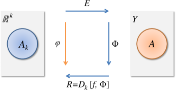
Figure 1. Definition of the map $\varphi$.

Remark 2.

Although $D_{k}$ is derived from what would commonly be termed an embedding theorem, we call $R$ a restriction, as it maps from an infinite dimensional domain into a finite-dimensional set, and $E$ an embedding, as it maps (or embeds) a finite-dimensional into an infinite dimensional space.

The map $E$ is obtained in two steps: Firstly, as $R$ is one-to-one on $A$, the requirement that

(7) $$R\circ\tilde{E}(x)=x\text{ for all }x\in A_{k}$$

uniquely defines a map $\tilde{E}:A_{k}\to A$. In a second step, we extend this map to a continuous map $E:\mathbb{R}^{k}\to Y$. To do this, we employ a generalization of the well-known Tietze extension theorem [9, I.5.3] found by Dugundji [8, Theorem 4.1], stated here with notation adapted to our needs:

Theorem 3.1.

Let $X$ be an arbitrary metric space and $\mathcal{A}\subset X$ be closed, $V$ a locally convex linear space and $p:\mathcal{A}\to V$ be continuous. Then there is a continuous map $P:X\to V$ with $P_{|\mathcal{A}}=p$ such that $P(X)$ is contained in the convex hull of $p(\mathcal{A})$.

Using this theorem in the situation introduced above, we obtain the following

Proposition 1.

There is a continuous map $\varphi:\mathbb{R}^{k}\to\mathbb{R}^{k}$ satisfying

(8) $$\varphi(R(u))=R(\Phi(u))\text{ for all }u\in A.$$

Proof.

By construction, the map $R:Y\to\mathbb{R}^{k}$ given by (3) is continuous (even Lipschitz) and one-to-one. Thus, restricting $R$ to $A$ we obtain a bijective map $\tilde{R}:A\to A_{k}$. As $A$ is assumed to be compact and $A_{k}\subset\mathbb{R}^{k}$ is Hausdorff, $\tilde{R}$ is a homeomorphism by a well-known theorem from elementary topology (see e. g. [26, Theorem 17.14]). Thus we obtain a continuous map $\tilde{E}:A_{k}\to A$ as $\tilde{E}=\tilde{R}^{-1}$.

As $Y$ is a normed linear space, it is locally convex. Thus we can apply Dugundji’s Theorem with $X=\mathbb{R}^{k}$, $\mathcal{A}=A_{k}$, $p=\tilde{E}$ and $V=Y$ to see that there is a continuous map $E:\mathbb{R}^{k}\to Y$ with $E_{|A_{k}}=\tilde{E}$. Finally, defining $\varphi$ through  (5) we obtain that $\varphi$ is continuous as a composition of continous maps. ∎

Now we are in a position to approximate the embedded invariant set $A_{k}$ via the corresponding dynamical system

(9) $$x_{j+1}=\varphi(x_{j})\quad j=0,1,\ldots.$$

To this end, we employ a subdivision scheme as defined in [5].

3.2. Subdivision Scheme

We briefly review the classical subdivision procedure. Let $Q\subset\mathbb{R}^{k}$ be a compact set. We define the global attractor relative to $Q$ by

(10) $$A_{Q}=\bigcap_{j\geq 0}\varphi^{j}(Q).$$

The subdivision procedure allows us to approximate this set. Roughly speaking, the idea of the algorithm is as follows. We start with a finite family of (large) compact subsets of $\mathbb{R}^{k}$ which cover the domain in which we want to analyze the dynamical behavior. Then we subdivide each of these sets into smaller ones and throw away subsets which do not contain part of the relative global attractor. Continuing the process with the new collection of (smaller) sets it becomes intuitively clear that this should lead to a successively finer approximation of the relative global attractor.

Let us be more precise. The algorithm generates a sequence ${\mathcal{B}}_{0},{\mathcal{B}}_{1},\ldots$ of finite collections of compact subsets of $\mathbb{R}^{k}$ such that the diameter

$$\mathop{\rm diam}\nolimits({\mathcal{B}}_{\ell})=\max_{B\in{\mathcal{B}}_{\ell}}\mathop{\rm diam}\nolimits(B)$$

converges to zero for $\ell\rightarrow\infty$. Given an initial collection ${\mathcal{B}}_{0}$, we inductively obtain ${\mathcal{B}}_{\ell}$ from ${\mathcal{B}}_{\ell-1}$ for $\ell=1,2,\ldots$ in two steps.

1. Subdivision: Construct a new collection $\hat{\mathcal{B}}_{\ell}$ such that

   (11) $$\bigcup_{B\in\hat{\mathcal{B}}_{\ell}}B=\bigcup_{B\in{\mathcal{B}}_{\ell-1}}B$$

   and

   (12) $$\mathop{\rm diam}\nolimits(\hat{\mathcal{B}}_{\ell})=\theta_{\ell}\mathop{\rm diam}\nolimits({\mathcal{B}}_{\ell-1}),$$

   where $0<\theta_{\min}\leq\theta_{\ell}\leq\theta_{\max}<1$.

2. Selection: Define the new collection ${\mathcal{B}}_{\ell}$ by

   (13) $${\mathcal{B}}_{\ell}=\left\{B\in\hat{\mathcal{B}}_{\ell}:\exists\hat{B}\in\hat{\mathcal{B}}_{\ell}\leavevmode\nobreak\ \mbox{such that}\leavevmode\nobreak\ \varphi^{-1}(B)\cap\hat{B}\neq\emptyset\right\}.$$

The first step guarantees that the collections ${\mathcal{B}}_{\ell}$ consist of successively finer sets for increasing $\ell$. In fact, by construction

$$\mathop{\rm diam}\nolimits({\mathcal{B}}_{\ell})\leq\theta_{\max}^{\ell}\mathop{\rm diam}\nolimits({\mathcal{B}}_{0})\rightarrow 0\quad\mbox{for $\ell\rightarrow\infty$.}$$

In the second step we remove each subset whose preimage does neither intersect itself nor any other subset in $\hat{\mathcal{B}}_{\ell}$. As we shall see, this step is responsible for the fact that the unions $\bigcup_{B\in{\mathcal{B}}_{\ell}}B$ approach the relative global attractor.

Denote by $Q_{\ell}$ the collection of compact subsets obtained after $\ell$ subdivision steps, that is,

$$Q_{\ell}=\bigcup_{B\in{\mathcal{B}}_{\ell}}B.$$

Moreover let ${\mathcal{B}}_{0}$ be a finite collection of closed subsets with $Q_{0}=\bigcup_{B\in{\mathcal{B}}_{0}}B=Q$. Then the main convergence result of [5] states that

$$\lim\limits_{k\rightarrow\infty}h\left(A_{Q},Q_{k}\right)=0,$$

where $h(B,C)$ is the usual Hausdorff distance between two compact subsets $B,C\subset\mathbb{R}^{n}$. However, in that work the authors assume that $\varphi$ is a homeomorphism and not just continuous, as in the situation here. For this reason, in the following we present a proof of convergence for continuous $\varphi$.

3.3. Proof of Convergence

Essentially, we will be able to follow the structure of the proof in [5]. However, there are some technical differences, and we will need one additional assumption on $A_{Q}$.

We begin with the following observation:

Lemma 3.2.

Suppose that $B\subset Q$ satisfies $B\subset\varphi(B)$. Then $B\subset A_{Q}$.

Proof.

From $B\subset\varphi(B)$ it follows that $\varphi^{j}(B)\subset\varphi^{j+1}(B)$ for all $j\geq 0$. Hence

$$B=\bigcap_{j\geq 0}\varphi^{j}(B)\subset\bigcap_{j\geq 0}\varphi^{j}(Q)=A_{Q}.$$

∎

We now can prove our first result.

Proposition 2.

Let $A_{Q}$ be the global attractor relative to the compact set $Q$, and suppose that the embedded attractor $A_{k}$ satisfies $A_{k}\subset Q$. Then

(14) $$A_{k}\subset A_{Q}.$$

Proof.

By construction of our dynamical system (see (5)–(7)), we have $\varphi(A_{k})=A_{k}$. Thus, Lemma 3.2 implies that $A_{k}\subset A_{Q}$. ∎

Remark 3.

Observe that we can in general not expect that $A_{k}=A_{Q}$. In fact, by construction $A_{Q}$ may contain several invariant sets and related heteroclinic connections. In this sense $A_{k}$ will be embedded in $A_{Q}$.

Next observe that the $Q_{\ell}$’s define a nested sequence of compact sets, that is, $Q_{\ell+1}\subset Q_{\ell}$. Therefore, for each $m$,

(15) $$Q_{m}=\bigcap\limits_{\ell=1}^{m}Q_{\ell},$$

and we may view

(16) $$Q_{\infty}=\bigcap\limits_{\ell=1}^{\infty}Q_{\ell}$$

as the limit of the $Q_{\ell}$’s.

Now we will prove the convergence of the subdivision scheme for continuous $\varphi$. More precisely we will show that $Q_{\infty}=A_{Q}$. This will be done in two steps. The first is

Lemma 3.3.

$$Q_{\infty}\subset A_{Q}.$$

Proof.

We will show that

$$Q_{\infty}\subset\varphi(Q_{\infty}).$$

Then the result follows with Lemma 3.2.

Let $y\in Q_{\infty}$. Then for every $\ell\geq 0$ there is a unique $B_{\ell}(y)\in{\mathcal{B}}_{\ell}$ with $y\in B_{\ell}(y)$. By the selection step of the subdivision scheme (see (13)), there is $z_{\ell}\in Q_{\ell}$ with $\varphi(z_{\ell})\in B_{\ell}(y)$. Choosing a convergent subsequence of $(z_{\ell})$, if necessary, we may assume that $z=\lim_{\ell\to\infty}z_{\ell}$. By construction, $z\in Q_{\infty}$, and since $\lim_{\ell\to\infty}\mathop{\rm diam}\nolimits(B_{\ell}(y))=0$ we conclude that $\lim_{\ell\to\infty}\varphi(z_{\ell})=y$. Finally $\varphi$ is continuous, and therefore $y=\varphi(z)$. Hence $y\in\varphi(Q_{\infty})$. ∎

For the inverse inclusion, we need to introduce an additional assumption, namely that $\varphi^{-1}(A_{Q})\subset A_{Q}$. This is automatically satisfied in the case where $\varphi$ is a homeomorphism. Moreover if $A_{k}$ is attracting and $A_{k}=A_{Q}$ then $A_{Q}$ is backward invariant. These observations justify this assumption.

Lemma 3.4.

Suppose that $\varphi^{-1}(A_{Q})\subset A_{Q}$, then

$$A_{Q}\subset Q_{\infty}.$$

This proof is identical to the proof of Lemma 3.2 in [5]. Thus, we will not restate it here.

We summarize the convergence result in the following

Proposition 3.

Suppose that the relative global attractor $A_{Q}$ satisfies $\varphi^{-1}(A_{Q})\subset A_{Q}$. Then

$$A_{Q}=Q_{\infty}.$$

3.4. Approximation of Attracting Sets

Observe that by construction of $\varphi$, the set $A_{Q}$ defined in Section 3.2 contains the one-to-one image $A_{k}$ of the invariant set $A$ of $\Phi$. We now show that by using sufficiently high powers of $\Phi$ we can actually approximate a one-to-one image of $A$ if $A$ is attracting.

Therefore, we now assume that $A$ is an attracting set, that is, $A$ attracts all bounded sets within a neighborhood $U$ of $A$. Moreover we assume that the set $Q$ is chosen in such a way that

(17) $$A_{k}\subset Q\quad\mbox{and}\quad E(Q)\subset U.$$

Hence, for every $x\in Q$, $\Phi^{j}(E(x))$ will eventually approach the attracting set $A$ for $j\to\infty$. However, this alone does not guarantee that $A_{k}$ is also an attracting set for the dynamical system $\varphi$. For instance, it may be the case that for a certain $\bar{x}\in Q$ one has a “spurious fixed point” in the sense that

$$\bar{x}=\varphi(\bar{x})$$

although $\Phi(E(\bar{x}))\not=E(\bar{x})$ may be closer to $A$ than $E(\bar{x})$.

In order to overcome this problem we now define for $m\geq 1$ the continuous maps

(18) $$\varphi_{m}=R\circ\Phi^{m}\circ E$$

and denote the corresponding relative global attractors by $A^{m}_{Q}$.

Remark 4.

Observe that $A$ is an invariant set for $\Phi^{m}$ for every $m$ and therefore we can still use $R$ as the restriction in our construction of the dynamical system $\varphi^{m}$.

Lemma 3.5.

$A_{k}\subset A^{m}_{Q}$ for all $m\geq 1$.

Proof.

Since $\Phi(A)=A$ we have $\varphi_{m}(A_{k})=A_{k}$ for $m\geq 1$. Moreover $A_{k}\subset Q$ (see (17)), and Lemma 3.2 implies that $A_{k}\subset A^{m}_{Q}$. ∎

Define

$$A^{\infty}_{Q}=\bigcap_{m\geq 1}A^{m}_{Q}.$$

Obviously $A_{k}\subset A^{\infty}_{Q}$. Moreover we have

Proposition 4.

$A_{k}=A^{\infty}_{Q}$.

Proof.

Suppose that $x\in A^{\infty}_{Q}\setminus A_{k}$. As $A_{k}$ is compact, this implies $\mbox{dist}(x,A_{k})=\epsilon>0$. As $A$ is compact, $R$ is continuous and $A_{k}=R(A)$, there is $\delta>0$ such that

$$\mbox{dist}(u,A)<\delta\Rightarrow\mbox{dist}(R(u),A_{k}))<\frac{\epsilon}{2}.$$

Set $V=E(Q)\subset U$ by assumption (see (17)). Since $A$ is attracting and $V$ is a compact set within $U$ we can find an $m\geq 1$ such that

$$h(\Phi^{m}(V),A)<\delta,$$

where $h$ is the Hausdorff distance. By our choice of $\delta$ it follows that

$$h(R(\Phi^{m}(V)),A_{k})=h(\varphi_{m}(Q),A_{k})<\frac{\epsilon}{2}.$$

Thus,

$$x\not\in\varphi_{m}(Q)\Rightarrow x\not\in A^{m}_{Q}\Rightarrow x\not\in A^{\infty}_{Q}$$

yielding a contradiction. ∎

Remark 5.

Roughly speaking Proposition 4 states that it will be possible to approximate an attracting set for $\Phi$ if we perform the computations with appropriately high iterates of $\Phi$.

4. Numerical Realization for Delay Differential Equations

As one important setting where finite dimensional dynamical phenomena occur in infinite dimensional Banach spaces, we consider delay differential equations with constant time delay $\tau>0$. More precisely we consider equations of the form

(19) $$\dot{y}(t)=g(y(t),y(t-\tau)),$$

where $y(t)\in\mathbb{R}^{n}$ and $g:\mathbb{R}^{n}\times\mathbb{R}^{n}\rightarrow\mathbb{R}^{n}$ is a smooth map. Following [14], we denote by ${\mathcal{C}}=C([-\tau,0],\mathbb{R}^{n})$ the (infinite dimensional) state space of the dynamical system (19). Equipped with the maximum norm, ${\mathcal{C}}$ is a Banach space.

Let $y_{u}(t)$ be the trajectory generated by (19) with the initial condition $u\in{\mathcal{C}}$. Then the flow $\Phi^{s}:{\mathcal{C}}\to{\mathcal{C}}$ of (19) is given by

$$u\mapsto\Phi^{s}(u),\mbox{ where $\Phi^{s}(u)(t)=y_{u}(s-t)$ for $t\in[-\tau,0]$.}$$

Next we fix $\omega>0$ and consider the corresponding time-$\omega$-map $\Phi^{\omega}:{\mathcal{C}}\to{\mathcal{C}}$ as our dynamical system. That is, we set

(20) $$\Phi=\Phi^{\omega}\quad\mbox{and}\quad Y={\mathcal{C}}$$

in our abstract dynamical system (1).

In order to numerically realize the construction of the map $\varphi=R\circ\Phi\circ E$ described in Section 3, we have to work on three tasks: the implementation of $E$, of $R$, and of $\Phi^{\omega}$ respectively. For the latter we will rely on standard methods for forward time integration of DDEs [2]. The map $R$ will be realized on the basis of Theorem 2.5 and Remark 1 by an appropriate choice of observables. For the numerical construction of the embedding $E$ we will employ a bootstrapping method that re-uses results of previous computations. This way we will in particular guarantee that the identities in (6) are at least approximately satisfied.

From now on we assume that upper bounds for both the box counting dimension $d$ and the thickness exponent $\sigma$ are available. This allows us to fix $k>2(1+\sigma)d$ according to Theorem 2.5.

4.1. Numerical Realization of $R$

For the definition of $R$ we have to specify the time span $\omega$ and appropriate corresponding observables. In the case of a scalar equation ($n=1$) we choose the observable $f$ to be

$$f(u)=u(-\tau).$$

Thus, in this case the restriction $R$ is simply given by

$$R=D_{k}[f,\Phi](u)=(u(-\tau),\Phi(u(-\tau)),\ldots,\Phi^{k-1}(u(-\tau)))^{T}.$$

The time span $\omega$ (see (20)) is defined to be a natural fraction of $\tau$, that is

(21) $$\omega=\frac{\tau}{K}\mbox{ for }K\in\mathbb{N}.$$

Remark 6.

• Observe that a natural choice for $K$ in (21) would be $K=k-1$ for $k>1$. That is, for each evaluation of $R$ the observable would be applied to a function $u:[-\tau,0]\rightarrow\mathbb{R}$ at $k$ equally distributed time steps within the interval $[-\tau,0]$.

• As described in Section 3.4 (see Remark 4) we will frequently replace $\Phi$ by $\Phi^{m}$ ($m>1$) in order to speed up the convergence towards the invariant sets $A$ resp. $A_{k}$. For an illustration of this procedure see Figure 2.

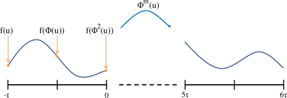
Figure 2. Numerical realization of the restriction $R$ for $n=1$, $K=2$ and $m=6K$.

For the numerical analysis of systems of delay differential equations ($n>1$) we make use of Remark 1 as follows: For each component $u_{j}$ of $u$ we define a separate observable $f_{j}$ $(j=1,\ldots,n)$ by

(22) $$f_{j}(u)=u_{j}(\nu_{j})\quad\mbox{for a $\nu_{j}\in[-\tau,0]$,}$$

and choose different time spans

(23) $$\omega_{j}=\frac{\tau}{K_{j}}\mbox{ for }K_{j}\in\mathbb{N}$$

accordingly.

Finally, we note that also more general constructions for the restriction $R:{\mathcal{C}}\to\mathbb{R}^{k}$ can be employed. In fact, by virtue of Theorem 2.4, for any $k$ that is sufficiently large for the delay embedding construction, an arbitrary linear map ${\mathcal{C}}\to\mathbb{R}^{k}$ will generically be one-to-one on $A$. Therefore almost every linear combination of trajectory points computed during forward integration can be used for the construction of the map $R$.

4.2. Numerical Realization of $E$

In the application of the subdivision scheme for the computation of the relative global attractor $A_{k}$ described in Section 3.2 one has to perform the selection step

$${\mathcal{B}}_{\ell}=\left\{B\in\hat{\mathcal{B}}_{\ell}:\exists\hat{B}\in\hat{\mathcal{B}}_{\ell}\leavevmode\nobreak\ \mbox{such that}\leavevmode\nobreak\ \varphi^{-1}(B)\cap\hat{B}\neq\emptyset\right\}$$

(see (13)). Numerically this is realized as follows: At first $\varphi$ is evaluated for a large number of test points $z_{j}^{k}\in B_{k}$ for each box $B_{k}\in\hat{\mathcal{B}}_{\ell}$. Then a box $B_{m}$ is kept in the collection ${\mathcal{B}}_{\ell}$ if it is hit by (at least) one of the images $\varphi(z_{\tilde{j}}^{\tilde{k}})$.

Remark 7.

In practice the test points $z_{j}^{k}\in B_{k}$ can be chosen according to several different strategies: In low dimensional problems one can choose them from a regular grid within each box $B_{k}$. Alternatively one can select the test points from the boundaries of the boxes. In our computations we have sampled a fixed number of test points from each box at random with respect to a uniform distribution.

For the evaluation of $\varphi=R\circ\Phi\circ E$ at a test point $z$ we need to define the image $E(z)$, that is, we need to generate adequate initial conditions for the forward integration of the DDE (19). In the first step of the subdivision procedure, when no information on $A$ is available, we proceed as follows. In the case of a scalar delay equation, that is $n=1$, we construct a piecewise linear function $u=E(z)$, where

(24) $$u(t_{i})=z_{i},$$

for $t_{i}=-\tau+i\cdot\omega,\ i=0,\dots,k-1$. Observe that by this choice of $E$ and $R$ the condition $R\circ E(z)=z$ is satisfied for each test point $z$ (see (6) and Remark 6 (a)).

For $n>1$ we proceed analogously and distribute the components of $z\in\mathbb{R}^{k}$ to the components $u_{j}$ of $u=E(z)\in\mathbb{R}^{n}$ according to (22) and (23). Also in this case the condition $R\circ E(z)=z$ still holds.

In the following steps of the subdivision procedure we proceed as follows: Note that if $B\in{\mathcal{B}}_{\ell}$, then, by the selection step, there must have been a $\hat{B}\in{\mathcal{B}}_{\ell-1}$ such that $R(\Phi^{\omega}(E(\hat{z})))\in B$ for at least one test point $\hat{z}\in\hat{B}$. Therefore, we can use the information from the computation of $\Phi^{\omega}(E(\hat{z}))$ to construct an appropriate $E(z)$ for each test point $z\in B$.

More concretely, in every step of the subdivision procedure, for every set $B\in{\mathcal{B}}_{\ell}$ we keep additional information about the points $\Phi^{\omega}(E(\hat{z}))$ that were mapped into $B$ by $R$ in the previous step. In the simplest case, we store $k_{i}\geq 1$ additional equally distributed function values for each interval $(-\tau+(i-1)\omega,-\tau+i\omega)$ for $i=1,\dots,k-1$. When $\varphi(B)$ is to be computed using test points from $B$, we first use the points in $B$ for which additional information is available and generate the corresponding initial value functions via spline interpolation. Note that the more information we store, the smaller the error $\|\Phi^{\omega}(E(\hat{z}))-E(z)\|$ becomes for $z=R(\Phi^{\omega}(E(\hat{z})))$. That is, we enforce an approximation of the identity $E\circ R(u)=u$ for all $u\in A$ (see (6)).

If the additional information is available only for a few points in $B$, we generate new test points in $B$ at random and construct corresponding trajectories by piecewise linear interpolation.

5. Numerical Results

In this section we present results of computations carried out for three different delay differential equations. In each case, $u(t)$ is scalar, although for the DDE considered in Section 5.2 the problem is recast into a three-dimensional form in order to obtain a first-order equation.

5.1. The Modified Wright Equation

As the first example, we consider a modification of the Wright equation,

(25) $$\dot{u}(t)=-\alpha\cdot u(t-1)\cdot[1-u^{2}(t)].$$

In [14] it has been shown that the stationary solution $u_{0}(t)\equiv 0$ undergoes a supercritical Hopf bifurcation at $\alpha=\pi/2$. Thus, (25) possesses a stable periodic solution for $\alpha>\pi/2$ – at least locally. In our computations we set $\alpha=2$, choose the embedding dimension $k=5$, and approximate the relative global attractor $A_{Q}\subset\mathbb{R}^{5}$ for $Q=[-2,2]^{5}$, see Figure 3. Here the set $A_{Q}$ consists of a reconstruction of the two-dimensional unstable manifold of $u_{0}\equiv 0$ which accumulates on a stable periodic orbit at its boundary.

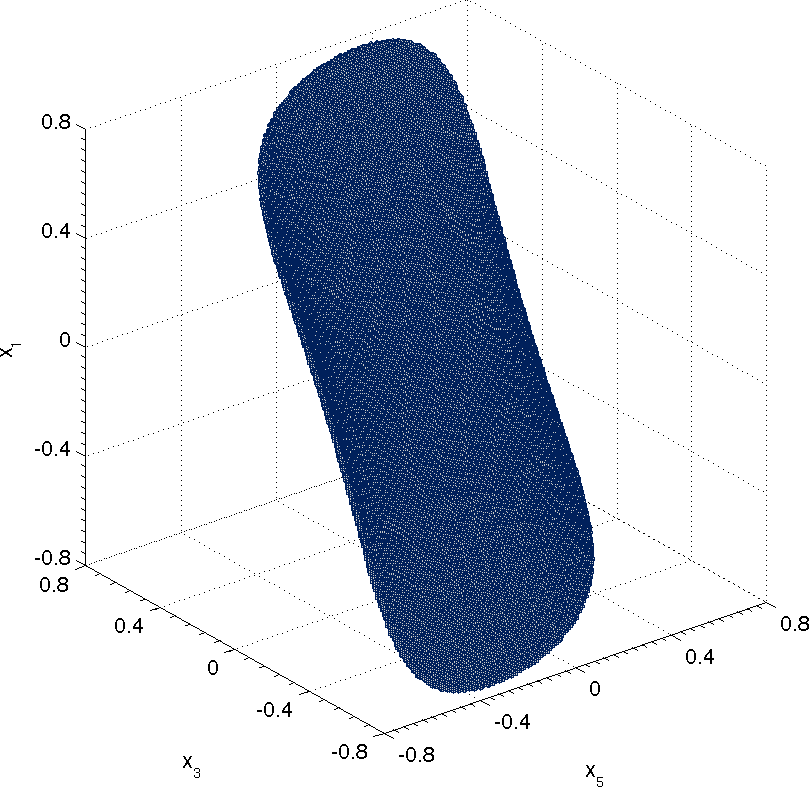
Figure 3. Three-dimensional projection of an approximation of the relative global attractor $A_{Q}$ within $Q=[-2,2]^{5}$ for equation (25) after $\ell=45$ subdivision steps (embedding dimension $k=5$ and iteration exponent $m=16$, see Section 4.1)

In Figure 4 we show box coverings of the reconstructed periodic solution itself. These have been obtained by removing a small open neighborhood $U$ of the origin from $Q=[-2,2]^{5}$ and computing $A_{\widetilde{Q}}$ for $\widetilde{Q}=Q\setminus U$.

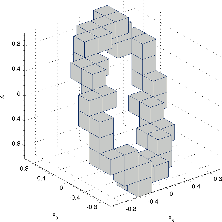
(a) $\ell=20$

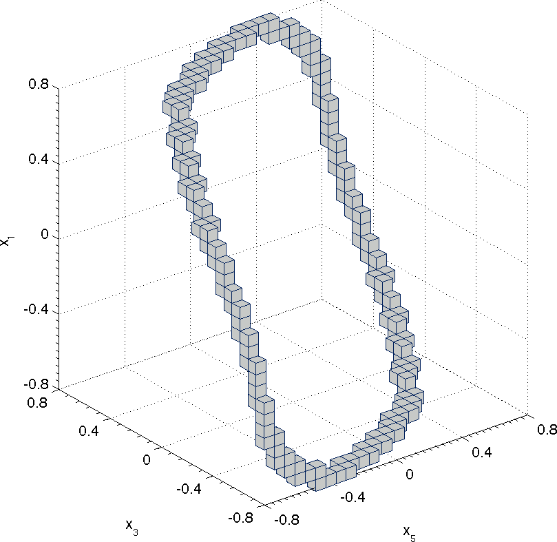
(b) $\ell=30$

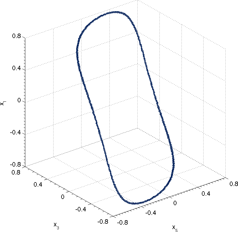
(c) $\ell=45$

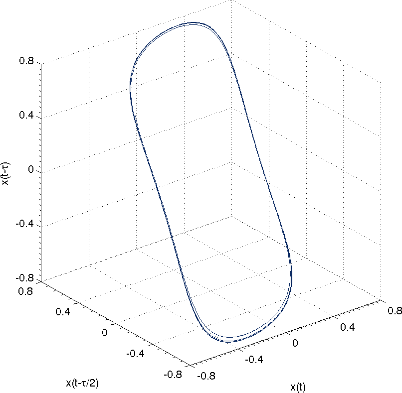
(d) Simulation

Figure 4. (a)-(c) Three-dimensional projections of successively finer coverings of the relative global attractor $A_{\widetilde{Q}}$ which corresponds to a reconstruction of a periodic orbit of (25). (d) Periodic orbit computed by direct simulation.

5.2. The Arneodo System with Delay

The second example is a modification of the Arneodo system [1] where a delay is introduced in the first order derivative of $u$,

$$\frac{d^{3}u}{dt^{3}}(t)+\frac{d^{2}u}{dt^{2}}(t)+2\frac{du}{dt}(t-\tau)-\alpha u(t)+u^{2}(t)=0.$$

This equation has been introduced and analyzed in [21]. In our computations we use the equivalent reformulation as a first-order system

$$\dot{u}_{1} =u_{2},$$

(26) $$\dot{u}_{2} =u_{3},$$

$$\dot{u}_{3} =-u_{3}-2u_{2}(t-\tau)+\alpha u_{1}-u_{1}^{2}.$$

The undelayed system (i. e. (26) with $\tau=0$) has been studied extensively. It possesses the equilibria $O_{1}=(0,0,0)$ and $O_{2}=(\alpha,0,0)$, the latter is asymptotically stable for $\alpha<2$. At $\alpha=2$ the equilibrium $O_{2}$ undergoes a supercritical Hopf bifurcation (cf. [16]). For values of $\alpha$ which are slightly larger than two, points on the two-dimensional unstable manifold of $O_{2}$ converge to the corresponding limit cycle on the branch of periodic solutions. That is, topologically speaking, we have the same situation as in Figure 3.

For the delayed (i. e. $\tau>0$) equation, the Hopf bifurcation occurs at decreasing values of $\alpha$ for increasing values of $\tau$. For fixed $\alpha=2.5$, the amplitude of the limit cycle grows with increasing values of $\tau$ and loses its stability in a period-doubling bifurcation at $\tau\approx 0.11$ [21]. Our purpose is to investigate the structure of the relative global attractor right after the occurrence of the period-doubling bifurcation. Concretely we set $\alpha=2.5$, $\tau=0.13$, choose the embedding dimension $k=5$, and approximate the relative global attractor $A_{Q}\subset\mathbb{R}^{5}$ for $Q=[-1,5]\times[-4,2]\times[-4,4]\times[-4,4]\times[-4,4]$. This way we compute a reconstruction of the two-dimensional unstable manifold of the origin which accumulates on a period-doubled limit cycle.

In this example we have made use of Remark 1 in our numerical realization. Concretely we have chosen $\omega=\tau/2$ and the following three observables (see (22) and (23))

$$f_{1}(u) = u_{2}(-\tau),\quad k_{1}=3,\quad K_{1}=2,$$

$$f_{2}(u) = u_{1}(0),\quad k_{2}=1,$$

$$f_{3}(u) = u_{3}(0),\quad k_{3}=1.$$

Thus, the restriction $R$ can be written as

$$R(u)=(u_{2}(-\tau),u_{2}(-\tau/2),u_{2}(0),u_{1}(0),u_{3}(0))^{T}$$

Observe that $R:{\mathcal{C}}\rightarrow\mathbb{R}^{5}$ is linear and therefore also Theorem 2.4 could be used in order to justify this construction. The corresponding reconstructions of the relative global attractor are shown in Figure 5.

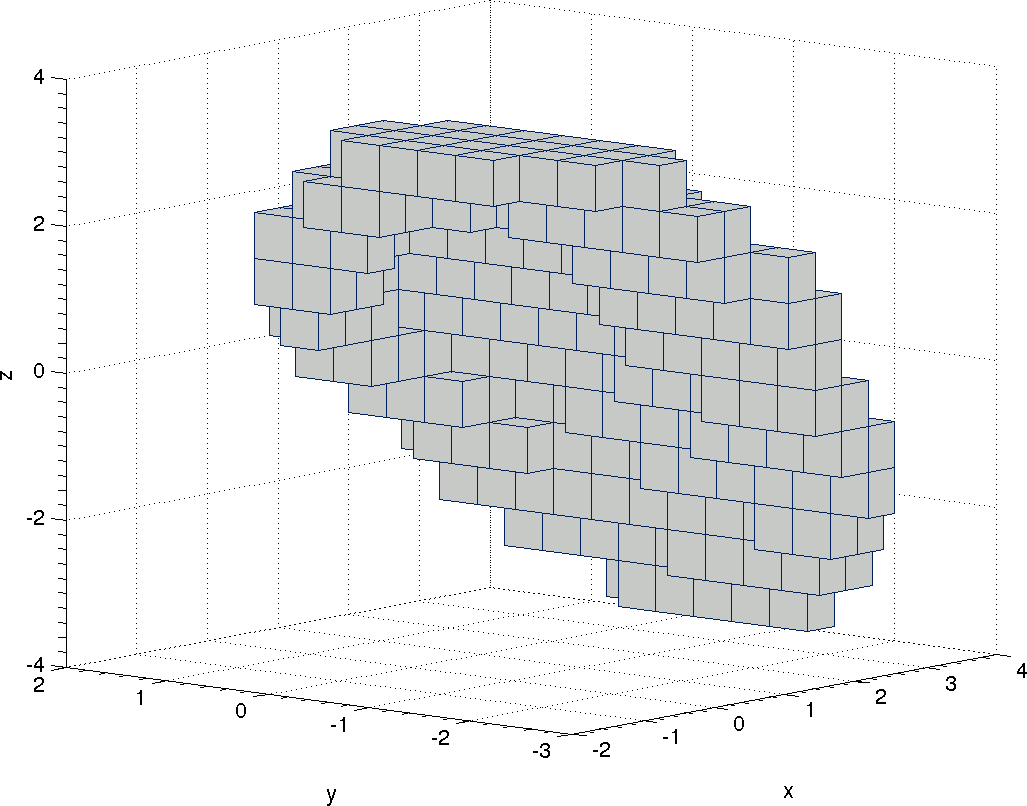
(a) $\ell=20$

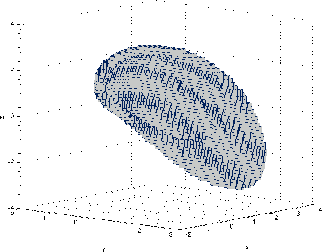
(b) $\ell=30$

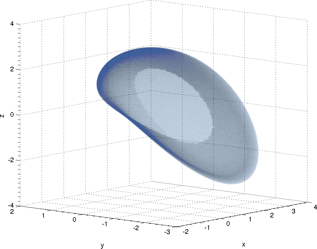
(c) $\ell=45$

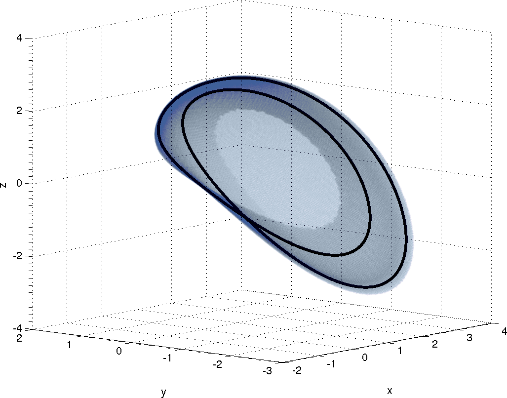
(d) $\ell=45$ with the period-doubled orbit computed by direct simulation

Figure 5. (a)-(d) Successively finer coverings of the relative global attractor for the Arneodo DDE (26) after $\ell$ subdivision steps ($\alpha=2.5$, $\tau=0.13$, embedding dimension $k=5$ and iteration exponent $m=15$; see Section 4.1).

Observe that after the period doubling bifurcation the relative global attractor contains a Moebius strip with the period-doubled periodic solution at its boundary. Thus, in the course of the period doubling bifurcation there has to occur a significant change of the geometry of the unstable manifold at its boundary so that it can accommodate the period-doubled solution. In fact, the corresponding mechanism has been analyzed analytically already in 1984 by Crawford and Omohundro [3]. It turns out that at the period doubling the unstable manifold starts to wrap itself “infinitesimally” around the unstable periodic solution. In a corresponding Poincaré section this becomes a spiraling behavior with very sharp curvature, and we analyze this behavior at the reconstruction in Figure 6 (see also Figure 16 in [3]). However, we expect that one would have to choose a much higher resolution (i. e. higher number of subdivisions) in order to reveal this dynamical behavior more clearly.

(a) Reconstructed unstable manifold. Red boxes (at $y=0$) illustrate the location of the Poincaré section.

(b) Poincaré section. Red circles mark the intersection with the period doubled periodic orbit.

(c) Zoom into the upper left corner of (b)

(d) Zoom into the lower right corner of (b)

Figure 6. Detailed illustration of a Poincaré section through the relative global attractor for (26).

5.3. The Mackey-Glass Equation

Our final example is the well-known delay differential equation introduced by Mackey and Glass in 1977 [18], namely

(27) $$\dot{u}(t)=\beta\frac{u(t-\tau)}{1+u(t-\tau)^{\eta}}-\gamma u(t),$$

where we choose $\beta=2,\gamma=1$, $\eta=9.65$, and $\tau=2$. This equation is a model of blood production, where $u(t)$ represents the concentration of blood at time $t$, $\dot{u}(t)$ represents production at time $t$ and $u(t-\tau)$ is the concentration at an earlier time, when the request for more blood is made. Direct numerical simulations indicate that the dimension of the corresponding attracting set is approximately $d=2$. Thus, we choose the embedding dimension $k=7$, and approximate the relative global attractor $A_{Q}$ for $Q=[0,1.5]^{7}\subset\mathbb{R}^{7}$. In Figure 7 we show projections of the coverings obtained after $\ell=28,42$ and $63$ subdivision steps as well as a direct simulation.

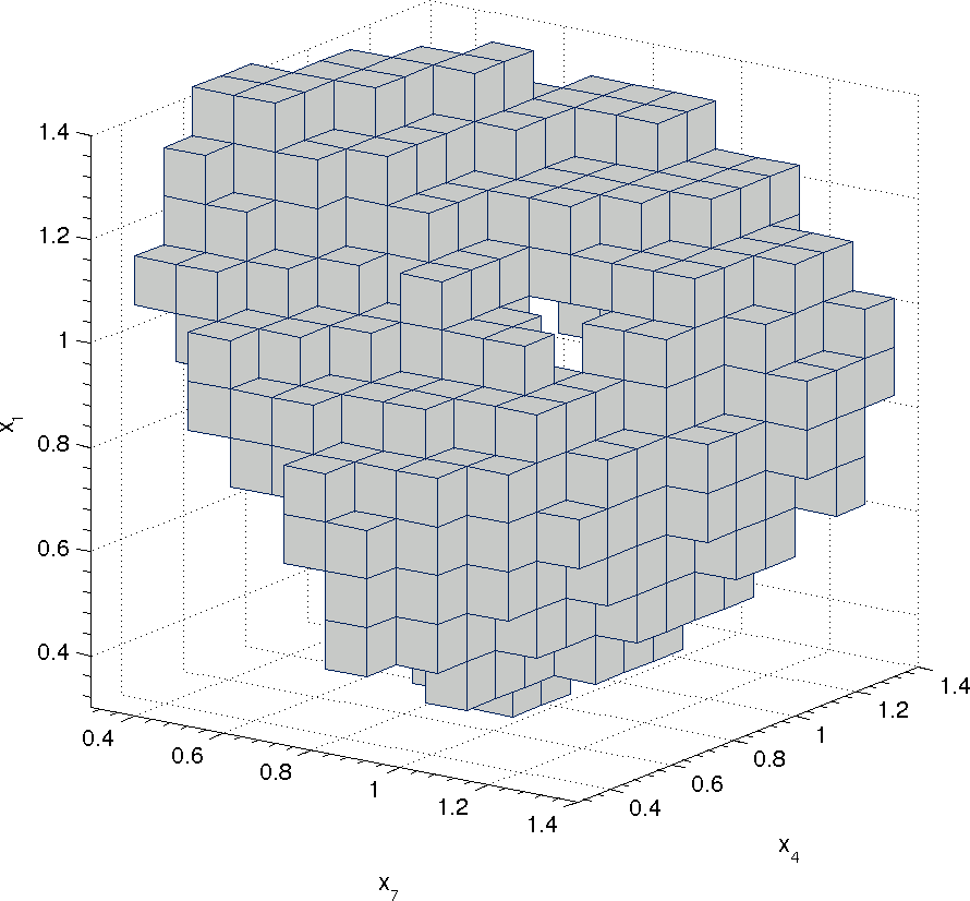
(a) $\ell=28$

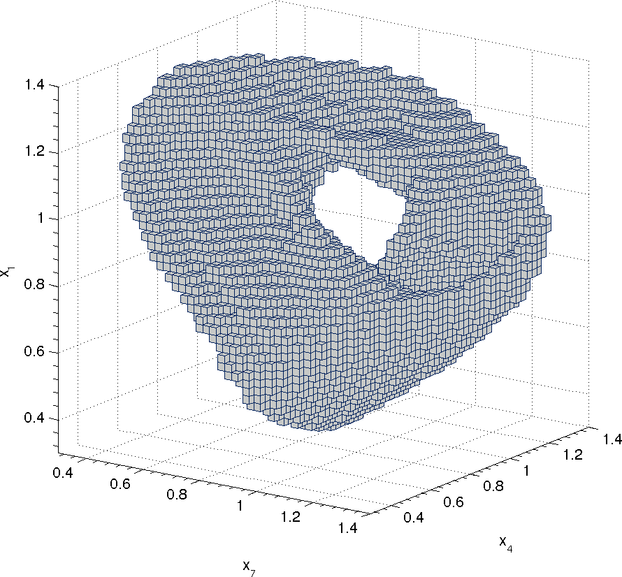
(b) $\ell=42$

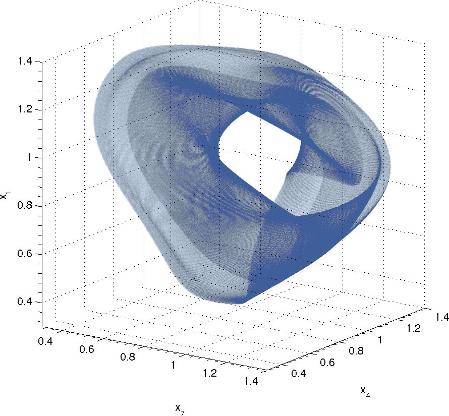
(c) $\ell=63$

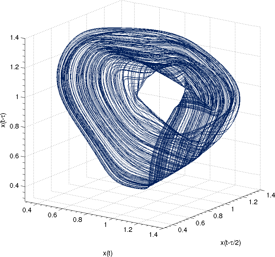
(d) Simulation

Figure 7. (a)-(c) Successively finer coverings of a relative global attractor after $\ell$ subdivision steps for the Mackey-Glass equation (27); (d) direct simulation.

Finally we conclude this section with an outlook and show a corresponding invariant measure for the reconstructed Mackey-Glass attractor in Figure 8. This measure has been computed with the software package GAIO [4] which is based on the techniques developed in [6]. However, a detailed investigation on how to approximate invariant measures in infinite dimensional problems efficiently using embedding theory will be done in future work.

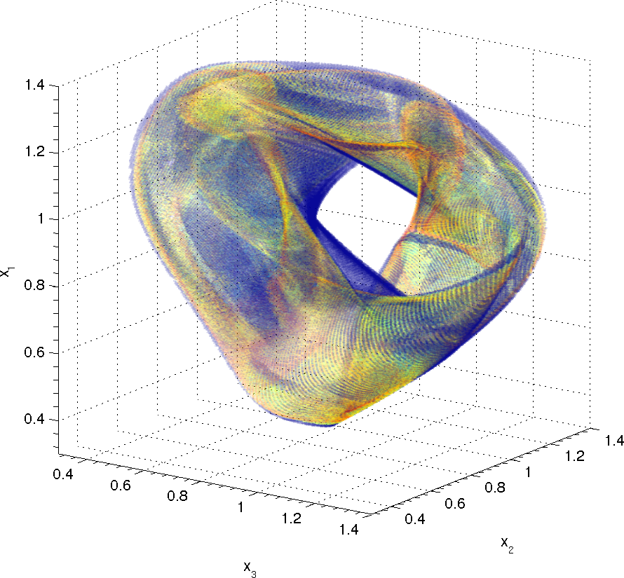
Figure 8. Invariant measure for the reconstructed Mackey-Glass attractor. The density ranges from blue (low density) $\rightarrow$ green $\rightarrow$ yellow $\rightarrow$ red (high density).

6. Conclusion

In contrast to the situation for finite dimensional dynamical systems, for which there exists a wide range of advanced numerical tools, there are currently only few options besides direct simulation for the numerical computation of attractors of infinite dimensional dynamical systems generated e. g. by DDEs. In this paper we develop a general methodology for the computation of finite dimensional compact attractors of infinite dimensional dynamical systems, and illustrate its application to several DDEs.

Combining the delay embedding technique with a set-oriented method for the computation of attractors, we obtain a flexible method for the analysis of infinite dimensional dynamical systems. More concretely, we use standard techniques for short-time simulation of the system in question to approximate the infinite dimensional dynamics, and employ the delay embedding technique on simulation results in order to obtain a representation of the dynamics by a continuous map on a moderately sized space. This map, in turn, can be analyzed using the subdivision scheme in order to compute a covering of an attractor. We show that in this way one obtains sets that are in one-to-one correspondence with the infinite dimensional attractor.

The method proposed shares vital characteristics with its counterparts for finite dimensional systems. Most importantly, the numerical effort essentially depends on the dimension of the object to be computed, and not on the dimension of ambient space used for computations, that is in the case of this paper, the dimension of the space used for the delay embedding. In three examples, we have illustrated the suitability for the computation of two-dimensional attractors. (In the case of the Mackey-Glass equation, the attractor probably even has a box counting dimension larger than $d=2.6$, see e.g. [10].) Furthermore, due to the set oriented nature of the underlying subdivision algorithm, the method does not depend on any special geometric properties (besides compactness) of the attractor.

References

- [1] A. Arneodo, Asymptotic Chaos, CNRS, Mécanique Statistique, Université de Nice, 1982.
- [2] A. Bellen and M. Zennaro, Numerical methods for delay differential equations, Oxford University Press, 2013.
- [3] J. D. Crawford and S. Omohundro, On the global structure of period doubling flows, Physica D: Nonlinear Phenomena, 13 (1984), 161 – 180, URL http://www.sciencedirect.com/science/article/pii/0167278984902756.
- [4] M. Dellnitz, G. Froyland and O. Junge, The algorithms behind GAIO — Set oriented numerical methods for dynamical systems, in Ergodic Theory, Analysis, and Efficient Simulation of Dynamical Systems, Springer-Verlag, Berlin, 2001, 145–174, 805–807.
- [5] M. Dellnitz and A. Hohmann, A subdivision algorithm for the computation of unstable manifolds and global attractors, Numerische Mathematik, 75 (1997), 293–317.
- [6] M. Dellnitz and O. Junge, On the Approximation of Complicated Dynamical Behavior, SIAM Journal on Numerical Analysis, 36 (1999), 491–515, URL http://epubs.siam.org/sinum/resource/1/sjnaam/v36/i2/p491_s1.
- [7] M. Dellnitz, O. Junge, M. Lo, J. E. Marsden, K. Padberg, R. Preis, S. Ross and B. Thiere, Transport of mars-crossing asteroids from the quasi-hilda region, Physical Review Letters, 94 (2005), 231102–1 – 231102–4.
- [8] J. Dugundji, An extension of Tietze’s theorem., Pacific J. Math., 1 (1951), 353–367, URL http://projecteuclid.org/euclid.pjm/1103052106.
- [9] N. Dunford and J. T. Schwartz, Linear Operators. Part I: General Theory, Interscience Publishers, Inc., 1957.
- [10] J. D. Farmer, Chaotic attractors of an infinite-dimensional dynamical system, Physica D, 4 (1982), 366.
- [11] G. Froyland and M. Dellnitz, Detecting and locating near-optimal almost invariant sets and cycles, SIAM Journal on Scientific Computing, 24 (2003), 1839–1863.
- [12] G. Froyland, C. Horenkamp, V. Rossi, N. Santitissadeekorn and A. Sen Gupta, Three-dimensional characterization and tracking of an agulhas ring, Ocean Modelling, 52-53 (2012), 69–75.
- [13] G. Froyland, S. Lloyd and N. Santitissadeekorn, Coherent sets for nonautonomous dynamical systems, Physica D, 239 (2010), 1527–1541.
- [14] J. K. Hale and S. M. Verduyn Lunel, Introduction to functional differential equations, Applied mathematical sciences, Springer-Verlag, New York, Berlin, Heidelberg, 1993.
- [15] B. R. Hunt and V. Y. Kaloshin, Regularity of embeddings of infinite-dimensional fractal sets into finite-dimensional spaces, Nonlinearity, 12 (1999), 1263, URL http://stacks.iop.org/0951-7715/12/i=5/a=303.
- [16] B. Krauskopf and H. Osinga, Two-dimensional global manifolds of vector fields, Chaos: An Interdisciplinary Journal of Nonlinear Science, 9 (1999), 768–774, URL http://scitation.aip.org/content/aip/journal/chaos/9/3/10.1063/1.166450.
- [17] I. Kukavica and J. C. Robinson, Distinguishing smooth functions by a finite number of point values, and a version of the takens embedding theorem, Physica D, 196 (2004), 45–66.
- [18] M. C. Mackey and L. Glass, Oscillation and chaos in physiological control systems, Science, 197 (1977), 287–289.
- [19] I. Mezić and A. Banaszuk, Comparison of systems with complex behavior, Physica D: Nonlinear Phenomena, 197 (2004), 101 – 133, URL http://www.sciencedirect.com/science/article/pii/S0167278904002507.
- [20] J. C. Robinson, A topological delay embedding theorem for infinite-dimensional dynamical systems, Nonlinearity, 18 (2005), 2135–2143.
- [21] T. Sahai and A. Vladimirsky, Numerical methods for approximating invariant manifolds of delayed systems, SIAM J. Applied Dynamical Systems, 8 (2009), 1116–1135, URL http://dx.doi.org/10.1137/080718772.
- [22] T. Sauer, J. A. Yorke and M. Casdagli, Embedology, J. Stat. Phys., 65 (1991), 579–616.
- [23] C. Schütte, W. Huisinga and P. Deuflhard, Transfer operator approach to conformational dynamics in biomolecular systems, in Ergodic Theory, Analysis, and Efficient Simulation of Dynamical Systems, Springer-Verlag, Berlin, 2001, 191–223.
- [24] J. Stark, Delay embeddings for forced systems. i. deterministic forcing, Journal of Nonlinear Science, 9 (1999), 255–332.
- [25] F. Takens, Detecting strange attractors in turbulence, Springer Lecture Notes in Mathematics, 898 (1981), 366–81.
- [26] S. Willard, General topology, Addison-Wesley, Reading, Mass. [u.a.], 1970.