Superconducting proximity effect in three-dimensional topological insulators in the presence of a magnetic field

Abstract

The proximity induced pair potential in a topological insulator-superconductor hybrid features an interesting superposition of a conventional spin-singlet component from the superconductor and a spin-triplet one induced by the surface state of the topological insulator. This singlet-triplet superposition can be altered by the presence of a magnetic field. We study the interplay between topological order and superconducting correlations performing a symmetry analysis of the induced pair potential, using Green functions techniques to theoretically describe ballistic junctions between superconductors and topological insulators under magnetic fields. We relate a change in the conductance from a gapped profile into one with a zero-energy peak with the transition into a topologically nontrivial regime where the odd-frequency triplet pairing becomes the dominant component in the pair potential. The nontrivial regime, which provides a signature of odd-frequency triplet superconductivity, is reached for an out-of-plane effective magnetization with strength comparable to the chemical potential of the superconductor or for an in-plane one, parallel to the normal-superconductor interface, with strength of the order of the superconducting gap. Strikingly, in the latter case, a misalignment with the interface yields an asymmetry with the energy in the conductance unless the total contribution of the topological surface state is considered.

I Introduction

A three-dimensional topological insulator (3DTI) is an extraordinary material with an insulating band gap but topologically protected gapless surface states. These states are possible due to spin-orbit interaction and follow a spin-polarized Dirac-type spectrum Qi and Zhang (2011). Among many unique properties of these materials, one has triggered an intense interest in the condensed matter community: the emergence of Majorana fermions when TIs are in electrical contact with a superconductor Alicea (2012); *Beenakker_Majorana. Indeed, the topological insulator-superconductor system can be used to engineer an effective spinless triplet superconductor which is expected to host zero-energy topologically protected Majorana bound states Fu and Kane (2008); *Sau_2010; *Lutchyn_2010; *Alicea_2010; *Oreg_2010; *Potter_2010; *Potter_2011; *Prada_2012; *Houzet_2013; *Tiwari_2013; *Tiwari_2014b; *Rex_2014.

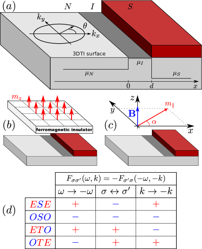
Figure 1: (a) Sketch of a normal-superconductor junction on the surface state of a topological insulator (regions $N$ and $S$, respectively) with an intermediate region $I$ modeled as a square potential barrier (see potential profile). The angle of incidence $\theta$ is measured with respect to the $x$-direction. (b) An out-of-plane magnetization $m_{z}$ is induced in the system by proximity from a ferromagnetic insulator. (c) An external magnetic field, stemming from the vector potential $\mathbf{A}$ (blue arrow) with arbitrary orientation, also generates an effective magnetization (red arrows). (d) Symmetry classification of the anomalous Green function $F_{\sigma\sigma^{\prime}}(\omega,\mathbf{k})$. With respect to the exchange of the time (frequency), spin, and spatial (momentum) coordinates, the Green function can be even (E) or odd (O). The spin part can be divided into a singlet (S) or three triplet (T) components. The Pauli principle allows for four different combinations; using a “frequency/spin/momentum” notation: ESE, OSO, ETO, and OTE.

Remarkably, the interplay between the spin-momentum locking at the surface of the 3DTI, the conventional pair potential from a superconductor, and magnetic order from either a ferromagnet or a magnetic field creates a very exotic induced pair potential in the 3DTI. First, the proximity induced pair potential from a conventional singlet $s$-wave superconductor on the surface of a 3DTI features a superposition of singlet and triplet states Read and Green (2000); Gor’kov and Rashba (2001); Schnyder et al. (2008); Yokoyama (2012); Tkachov and Hankiewicz (2013a); Tkachov (2013); Tkachov and Hankiewicz (2013b); Burset et al. (2014). Owing to the symmetry of Cooper pairs, the singlet (triplet) components are even (odd) under the exchange of the spatial coordinates of the two electrons (even/odd in momentum). At the same time, they are all even under the exchange of time coordinates (even in frequency). Second, at the interface between normal and superconducting regions inversion symmetry is broken. Such inhomogeneity generates new pairing components that are odd (even) in momentum if they are a singlet (triplet) state of spin Tanaka and Golubov (2007); *Eschrig_2007; *Tanaka_2007b; *Tanaka_2007c; *Tanaka_JPSJ; Yokoyama (2012); Black-Schaffer and Balatsky (2012); *Black-Schaffer_2013; *Black-Schaffer_2013b. Therefore, the Pauli principle imposes that these new terms must be odd in frequency. Finally, as we demonstrate in this paper, magnetic order directly affects all these components and opens the possibility for the exotic odd-frequency terms to become dominant and produce strong changes in transport observables of these systems.

Among the unconventional components of the pair potential, a new, very rare type of superconducting condensate can be induced in this system: one with a spin-triplet component that is odd in frequency and even in momentum Berezinskii (1974a); *Berezinskii_1974R; *Balatsky_1992. Such exotic odd-frequency triplet pairing has been proposed to explain the long-range proximity effect observed in superconductor-ferromagnet hybrids Bergeret et al. (2001); *Birge_2010. On such systems, the odd-frequency triplet component can be filtered from the rest of induced components of the superconducting condensate since it is the only one resistant to disorder [Formoreinformationaboutodd-frequencytripletpairingonferromagnet-superconductorhybridssee][]Bergeret_RMP; *Eschrig_2010. In topological systems, spin-polarization can be used to detect this unconventional pairing. Recently, Crépin et al. have proposed a detection scheme based on nonlocal conductance measurements on the one-dimensional edge of a two-dimensional TI Crépin et al. (2015). Moreover, odd-frequency triplet pairing and the emergence of Majorana bound states are related: any system that supports Majorana zero-energy bound states also develops an odd-frequency spin-triplet component of the pair potential Asano and Tanaka (2013); Stanev and Galitski (2014); Liu et al. (2015); Ebisu et al. (2015); Snelder et al. (2015a).

In this paper, we consider hybrid systems between 3DTI and superconductors like the one sketched in Fig. 1(a). We study the proximity effect when such systems are exposed to a magnetization extended over the whole junction. The magnetization can be induced by proximity to a ferromagnetic material (b) or by an external magnetic field (c). Previous works on 3DTI-based normal-superconductor (NS) and Josephson (SNS) junctions focused only on transport signatures of such hybrids and the conditions for the formation of Majorana bound states Tanaka et al. (2009a); *Linder_2010b; *Sengupta_2013; Linder et al. (2010b); Olund and Zhao (2012); Snelder et al. (2013); Tkachov (2013); Tkachov and Hankiewicz (2013b); Nussbaum et al. (2014); Lu et al. (2015a, b). Here, we study the interplay between topological order and superconducting correlations performing a symmetry analysis of the induced pair potential based on the anomalous Green function. We go beyond previous works Yokoyama (2012); Black-Schaffer and Balatsky (2012); *Black-Schaffer_2013; *Black-Schaffer_2013b by including the effect of the magnetization on the superconducting electrode Tkachov et al. (2015).

In the absence of magnetization, singlet and triplet components of the pair potential with even and odd frequency dependences are created at the TI-superconductor interface. However, the even-frequency singlet component is dominant and no low-energy states are formed Black-Schaffer and Balatsky (2012); *Black-Schaffer_2013; *Black-Schaffer_2013b. For finite magnetization, the odd-frequency triplet components can become dominant, resulting in a rich subgap structure with emerging low-energy peaks. We study their effect on the NIS conductance, with I an intermediate region, and the local density of states (LDOS) for two orientations of the magnetization: in- and out-of-plane. For the latter, when the strength of the magnetization approaches the magnitude of the chemical potential in the superconductor, the odd-frequency triplet component becomes stronger than the singlet one. Consequently, a zero-energy peak emerges in the NIS conductance. We find the same behavior for in-plane case with strength comparable to the superconducting gap and oriented parallel to the NIS interface. When the in-plane magnetization is oriented differently, the rotational invariance of the band structure is broken. As a consequence, the NIS conductance becomes asymmetric with the energy; a feature completely different to previous works based on ferromagnet-superconductor junctions on 3DTIs Tanaka et al. (2009a); *Linder_2010b; Linder et al. (2010b); Lu et al. (2015a). Independently of the orientation of the in-plane magnetization, when its strength is comparable to the superconducting gap, the odd-frequency triplet component becomes similar to or bigger than the singlet one. Consequently, subgap resonances are present in the LDOS and NIS conductance.

This paper is organized as follows. We present the model for the TI-superconductor hybrid system and describe the effect of the magnetization in Sec. II. In Sec. III, we describe the symmetry classification of the induced pair potential and study the conditions for the emergence of new symmetry terms for finite magnetization, which we associate with changes in the local density of states. In Sec. IV, we connect the previous results with an experimentally relevant observable like the NIS conductance. We present our conclusions in Sec. V. Finally, in the Appendix, we describe our method to compute the retarded Green function and the transport observables that we examine.

II Model

In our setup, the surface of a 3DTI extends along the $x$-$y$ plane. The superconducting and intermediate regions are located, respectively, at $x>d$ and $0<x<d$ (see Fig. 1). The role of the intermediate region is to include any interface scattering between the normal and the superconducting regions. We thus assume perfectly flat and clean interfaces. The low-energy electron and hole excitations at the surface of the 3DTI are described by the Bogoliubov-de Gennes (BdG) equations $\check{H}\Psi=E\Psi$, with $E$ the excitation energy. Particle-hole symmetry imposes that if $\Psi_{E}$ is a solution of the BdG equations with excitation energy $E$, $\Psi_{-E}$ must also be a solution. In Nambu (particle-hole) and spin space, with basis $\Psi=[\hat{c}_{\uparrow}(\mathbf{k}),\hat{c}_{\downarrow}(\mathbf{k}),\hat{c}^{\dagger}_{\uparrow}(-\mathbf{k}),\hat{c}^{\dagger}_{\downarrow}(-\mathbf{k})]^{T}$, with $\hat{c}_{\sigma}(\mathbf{k})$ the annihilation operator for an electron of spin $\sigma=\uparrow,\downarrow$ and momentum $\mathbf{k}$, the Hamiltonian reads as

$$\check{H}=\left(\!\begin{array}[]{cc}\hat{h}(\mathbf{k})-\mu(x)\hat{\sigma}_{0}&i\hat{\sigma}_{2}\Delta(x)\\ -i\hat{\sigma}_{2}\Delta(x)&\mu(x)\hat{\sigma}_{0}-\hat{h}^{*}(-\mathbf{k})\end{array}\!\right)\quad,$$ (1)

where $\mu(x)$ is the chemical potential and the Pauli matrices $\hat{\sigma}_{0,1,2,3}$ act on spin space. We model the intermediate region as a square potential with thickness $d$ and height $\mu_{I}$, as it is shown in Fig. 1(a). Therefore, we have

$$\mu(x)=\left\{\begin{array}[]{cl}\mu_{N}&,x\leq 0\\ \mu_{I}&,0<x<d\\ \mu_{S}&,x\geq d\end{array}\right.\quad.$$

We note that, due to Klein tunneling, the barrier does not affect the normally incident modes (with $k_{y}\sim 0$) Tkachov and Hankiewicz (2013a); Tkachov (2013). The pair potential in the superconducting region is $\Delta(x)=\Delta\Theta(x-d)$, with $\Delta\geq 0$ and $\Theta(x)$ the Heaviside function. Electron-like quasiparticles are described by a Dirac Hamiltonian as

$$\hat{h}(\mathbf{k})=v_{F}\left(k_{x}\hat{\sigma}_{1}+k_{y}\hat{\sigma}_{2}\right)-e\mathbf{A}\cdot\mathbf{\hat{\sigma}}\quad,$$ (2)

with $v_{F}$ the Fermi velocity, $e$ the electron charge, and $\mathbf{A}$ the vector potential (we take $\hbar=1$ and $c=1$ for simplicity). For a constant magnetic field, the vector potential depends linearly on the spatial coordinates. In what follows, we describe two situations where we can neglect the spatial dependence of $\mathbf{A}$ and regard it as constant. The effect of a uniform constant $\mathbf{A}$ has the same form as a Zeeman interaction where the vector potential plays the role of an exchange field. Consequently, the Hamiltonian in Eq. (1) is equivalent to the one used in, e.g., Ref. Tanaka et al., 2009a, when we define an effective magnetization

$$\check{M}={} \left(\!\begin{array}[]{cc}\mathbf{m}\cdot\mathbf{\hat{\sigma}}&0\\ 0&-\mathbf{m}\cdot\mathbf{\hat{\sigma}}^{*}\end{array}\!\right)$$ (5)

$$={} -e\left[\left(A_{x}\hat{\sigma}_{1}+A_{z}\hat{\sigma}_{3}\right)\otimes\hat{\tau}_{3}+A_{y}\hat{\sigma}_{2}\otimes\hat{\tau}_{0}\right]\quad,$$

where the Pauli matrices $\tau_{0,1,2,3}$ act in Nambu space. The main difference with previous works Tanaka et al. (2009a); Linder et al. (2010a); Snelder et al. (2013) is that magnetic order is induced in the whole junction and is not just limited to an intermediate region. We consider this a sensible approach to describe 3DTI hybrid junctions where proximity-induced superconductivity on the two-dimensional surface state can be sensitive to magnetic effects.

With our choice of the reference frame (see Fig. 1), the momentum component parallel to the interface $k_{y}$ is conserved. Therefore, the solutions of the BdG equations are expressed as $\Psi(x,y)=\mathrm{e}^{ik_{y}y}\Psi(x,\theta)$, with $\sin\theta=k_{y}/|\mathbf{k}|$. A full list of the scattering states for this junction is presented in Appendix A. Next, we provide the main results for two different orientations of the effective magnetization $\check{M}$.

II.1 Out-of-plane effective magnetization

We start by considering an out-of-plane effective magnetization $\check{M}=m_{z}\hat{\sigma}_{3}\otimes\hat{\tau}_{3}$ (see Fig. 1), stemming from a magnetic field such that $\mathbf{A}=[0,0,A_{z}(x)]$. Ignoring the spatial dependence of the vector potential is equivalent to assume that the magnetization is a Zeeman term with exchange field $m_{z}$.

In the superconducting region, the positive branch of the low-energy spectrum is then given by

$$E_{\pm}(\mathbf{k})=\sqrt{\mu^{2}+\Delta^{2}+v_{F}^{2}|\mathbf{k}|^{2}+m_{z}^{2}\pm 2r_{Z}}\quad,$$ (6)

with $r_{Z}=\sqrt{\mu^{2}v_{F}^{2}|\mathbf{k}|^{2}+m_{z}^{2}\left(\mu^{2}+\Delta^{2}\right)}$. Although the energy spectrum looks rather complicated, its analysis is very simple if we focus on the $\Gamma$ point $\mathbf{k}=0$, where we find

$$E_{\pm}(0)=|m_{z}\pm\sqrt{\mu^{2}+\Delta^{2}}|\quad.$$

It is straightforward to see that both $m_{z}$ and the superconducting gap $\Delta$ independently open a gap in an otherwise gapless Dirac spectrum. When both $m_{z}$ and $\Delta$ are finite at the same time, a competition between the superconducting and the magnetic gap occurs. As a result, a zero-energy state can be created when $m_{z}^{2}=\mu^{2}+\Delta^{2}$. This allows us to define the effective superconducting gap

$$\Delta_{z}\equiv\Delta\sqrt{1-(m_{z}/|\mu|)^{2}}\quad.$$ (7)

For $0<m_{z}\leq\mu$, the gap is real and superconductivity is the dominant process in the superconducting region. On the other hand, superconductivity is suppressed by a magnetic gap when $m_{z}>\mu>\Delta$. The critical point between the two regimes is thus $m_{z}=\mu>\Delta$. The Fermi energy for 3DTIs based on Bi compounds or strained HgTe can be estimated as $\mu\gtrsim 50$ meV. A comparable exchange field can be obtained by proximity from a ferromagnetic insulator, as sketched in Fig. 1(b). In a recent experiment, EuS was deposited on top of the topological insulator Bi₂Se₃. Ferromagnetic order induced onto the surface of the TI was estimated to be around $(60-400)$ meV/area [nm²] per applied Tesla Wei et al. (2013). For small enough devices, this correction can be much larger than the induced superconducting gap on TIs for fields below the critical field of the superconductor.

II.2 In-plane effective magnetization

We now examine Eq. (5) in the heavily-doped, weak-field approximation with $\mu\gg|E|,\Delta,|\mathbf{m}|$. Since the out-of-plane component becomes relevant only when $m_{z}\sim\mu$, we can ignore it in this approximation. The resulting in-plane effective magnetization is $\hat{M}=m_{x}\hat{\sigma}_{1}\hat{\tau}_{3}+m_{y}\hat{\sigma}_{2}\hat{\tau}_{0}\equiv m_{\parallel}\left(\hat{\sigma}_{1}\hat{\tau}_{3}\cos\alpha+\hat{\sigma}_{2}\hat{\tau}_{0}\sin\alpha\right)$, with the angle $\alpha$ measured from the $k_{x}$ direction [see more details in Fig. 1(c)]. The in-plane effective magnetization is defined from the vector potential $\mathbf{A}=[A_{x}(z),A_{y}(z),0]$ which we approximate by its value at the junction’s plane. This approximation is also valid for the superconducting region if we let the penetration length of the superconductor be much larger than the superconducting coherence length Tkachov et al. (2015); Fogelström et al. (1997); *Tanaka_2002; *Tanaka_2009b.

In the superconducting region, the positive branch of the low-energy spectrum is given by

$$E_{\pm}(\mathbf{k})\approx\mathbf{n}\cdot\mathbf{m}\!+\!\sqrt{\left(\mu\pm v_{F}|\mathbf{k}|\right)^{2}+\Delta^{2}}\quad,$$ (8)

where we have defined $\mathbf{n}=\mathbf{k}/|\mathbf{k}|=(\cos\theta,\sin\theta,0)$. The effect of the weak field is a shift in the energy, analogous to the Doppler shift discussed for a SQUID-like geometry of helical edge states in Ref. Tkachov et al., 2015. Using that

$$\mathbf{n}\cdot\mathbf{m}=m_{\parallel}\left(\cos\theta\cos\alpha+\sin\theta\sin\alpha\right)=m_{\parallel}\cos\left(\theta-\alpha\right)\quad,$$

we can define the effective gaps

$$\Delta_{\pm}\equiv|\Delta\pm m_{\parallel}\cos\left(\theta-\alpha\right)|\quad.$$ (9)

The critical value for which the effective gap closes is now $m_{\parallel}\!\sim\!\Delta$, which can be reached with rather weak fields. The magnetic field induces a finite Cooper pair (condensate) momentum which affects quasiparticles differently depending on their direction of motion. Due to the spin-momentum locking at the surface state of the TI, quasiparticles moving in opposite directions feel reversed magnetic fields. In other words, they travel upstream or downstream with respect to the superconducting condensate. This asymmetric behavior with the direction of motion is not found in non-topological systems Fogelström et al. (1997); *Tanaka_2002; *Tanaka_2009b; Burset et al. (2009).

II.3 Retarded Green function and experimental observables

We now construct the retarded Green function associated to the Hamiltonian in Eq. (1). The retarded Green function is obtained combining all scattering states as McMillan (1968); *Furusaki_1991; *Tanaka_1996; *Kashiwaya_2000; *Herrera_2010

$$\check{G}^{r}(x,x^{\prime},E+i0^{+};\theta)=$$ (10)

$$\left\{\!\!\begin{array}[]{lr}\begin{array}[]{c}\alpha_{1}\Psi_{3}(x)\tilde{\Psi}_{1}^{T}(x^{\prime})\!+\!\alpha_{2}\Psi_{3}(x)\tilde{\Psi}_{2}^{T}(x^{\prime})\\ +\alpha_{3}\Psi_{4}(x)\tilde{\Psi}_{1}^{T}(x^{\prime})\!+\!\alpha_{4}\Psi_{4}(x)\tilde{\Psi}_{2}^{T}(x^{\prime})\end{array}\,,&x<x^{\prime}\\ \begin{array}[]{c}\beta_{1}\Psi_{1}(x)\tilde{\Psi}_{3}^{T}(x^{\prime})\!+\!\beta_{2}\Psi_{2}(x)\tilde{\Psi}_{3}^{T}(x^{\prime})\\ +\beta_{3}\Psi_{1}(x)\tilde{\Psi}_{4}^{T}(x^{\prime})\!+\!\beta_{4}\Psi_{2}(x)\tilde{\Psi}_{4}^{T}(x^{\prime})\end{array}\,,&x>x^{\prime}\end{array}\right.\quad.$$ (17)

An incoming electron (hole) from the normal region onto the superconductor can be (a) Andreev reflected as a hole (electron); (b) normal reflected as an electron (hole); (c) transmitted to the superconductor as an electronlike (holelike) quasiparticle; and (d) as a holelike (electronlike) quasiparticle. We label this scattering process with the number $1$ ($2$). The corresponding wave function is thus $\Psi_{1(2)}(x)$. Analogously, the equivalent process where the incoming particle is an electronlike (holelike) excitation incident from the superconductor is labeled with the number $3$ ($4$). In Appendix B, we show more details of the calculation of the Green function, the reflection amplitudes $a_{j}$, $b_{j}$, and the transmission amplitudes $c_{j}$ and $d_{j}$, with $j=1,\dots,4$. The wave functions $\tilde{\Psi}_{i}(x)$ correspond to the conjugate scattering processes to $\Psi_{i}(x)$. The coefficients $\alpha_{i}$ and $\beta_{i}$ are determined by the continuity equation obtained after integrating the BdG equations around $x=x^{\prime}$, namely,

$$\frac{-i}{v_{F}}\hat{\sigma}_{1}\otimes\hat{\tau}_{0}=$$ (18)

$$\check{G}^{r}(x,x+0^{+},E+i0^{+};\theta)-\check{G}^{r}(x,x-0^{+},E+i0^{+};\theta)\quad.$$

The spectral density of states is then calculated from the retarded Green function as

$$A(x,E;\theta)=-\frac{1}{\pi}\operatorname{Im}\left\{\mathrm{Tr}\check{G}_{ee}^{r}(x,x,E+i0^{+};\theta)\right\}\quad,$$

where the trace is taken on the electron-electron component of the Green function in Nambu space (i.e., the single-particle Green function). Furthermore, the local density of states (LDOS) is given by

$$\rho(x,E)=\int\limits_{-\pi/2}^{\pi/2}\!\!\!\mathrm{d}\theta\cos\theta A(x,E;\theta)\quad.$$ (19)

In the next sections, we normalize the LDOS in the superconductor by the LDOS calculated deep inside the normal region, $\rho_{N}(E)=|\mu_{N}+E|/v_{F}$ (see Appendix C for more details).

We define the conductance of the NIS junction as Blonder et al. (1982); Tanaka and Kashiwaya (1995)

$$G_{NS}(E)=\int\limits_{-\pi/2}^{\pi/2}\!\!\!\mathrm{d}\theta\cos\theta\left[1-|b_{1}(E,\theta)|^{2}+|a_{1}(E,\theta)|^{2}\right]\quad,$$ (20)

where $a_{1}(E,\theta)$ and $b_{1}(E,\theta)$ are the Andreev and normal reflection amplitudes, respectively, for an incident electron. We normalize the conductance using the constant value $G_{0}=G_{NS}(E\gg\Delta)$.

Notice that both the conductance and the LDOS are averaged over all incident angles, labeled by $\theta\in[-\pi/2,\pi/2]$ .

III Symmetry of the induced pair potential

Induced superconducting correlations are manifested in the anomalous Green function (the electron-hole component of the Green function in Nambu space), i.e., the $2\times 2$ matrix in spin space

$$\tilde{F}_{\sigma\sigma^{\prime}}(t_{1},\mathbf{r}_{1};t_{2},\mathbf{r}_{2})=\left\langle T_{t}\Psi_{\sigma}(t_{1},\mathbf{r}_{1})\Psi_{\sigma^{\prime}}(t_{2},\mathbf{r}_{2})\right\rangle\quad,$$

with $T_{t}$ the time-ordering operator and $\Psi_{\sigma}(t_{1},\mathbf{r}_{1})$ the fermion operator for given spin, time, and space coordinates. In homogeneous systems, we can define the relative coordinates $\mathbf{r}=\mathbf{r}_{1}-\mathbf{r}_{2}$ and $t=t_{1}-t_{2}$ and the Pauli principle imposes that $\tilde{F}_{\sigma\sigma^{\prime}}(t,\mathbf{r})=-\tilde{F}_{\sigma^{\prime}\sigma}(-t,-\mathbf{r})$. After Fourier transformations, we have

$$F_{\sigma\sigma^{\prime}}(\omega,\mathbf{k})=-F_{\sigma^{\prime}\sigma}(-\omega,-\mathbf{k})\quad.$$

We can write explicitly the spin-singlet and triplet components of the anomalous Green function in the basis of Eq. (1) as

$$\hat{F}(\omega,\mathbf{k})=\left[F_{0}(\omega,\mathbf{k})\hat{\sigma}_{0}+F_{j}(\omega,\mathbf{k})\hat{\sigma}_{j}\right]i\hat{\sigma}_{2}\quad.$$

Evidently, the Pauli principle must be fulfilled independently by the singlet and the three triplet components. With respect to the spin degree of freedom, the singlet component is odd and the triplet ones even. Under a sign change in either the frequency or the momentum, the functions $F_{\nu}(\omega,\mathbf{k})$, with $\nu=0,1,2,3$, can also be classified as even or odd. As a consequence, only four types of symmetries are allowed, namely, (i) Even-frequency spin-Singlet Even-parity (ESE); (ii) Even-frequency spin-Triplet Odd-parity (ETO); (iii) Odd-frequency spin-Singlet Odd-parity (OSO); and (iv) Odd-frequency spin-Triplet Even-parity (OTE) [see Fig. 1(b) and, for more details, Ref. Tanaka and Golubov, 2007; *Eschrig_2007; *Tanaka_2007b; *Tanaka_2007c; *Tanaka_JPSJ].

In our model, we assume perfectly flat and clean interfaces which conserve the parallel component of the momentum ($k_{y}$ for the axis choice in Fig. 1). In the quasi-one dimensional model, transport along these junctions is described by one-dimensional Green functions $\check{G}(x,x^{\prime},\omega;k_{y})$ separately for each channel $k_{y}$. For positive frequencies, we construct these Green functions using Eq. (10), which considers scattering solutions of the BdG equations with excitation energies $E\geq 0$. For negative frequencies, we need to consider the time-reversal of the scattering processes, i.e., the $E<0$ solutions of the BdG equations, which are provided by the advanced Green function. Therefore, to study the frequency dependence of the anomalous Green function, we combine the retarded and the advanced Green functions as

$$F_{\nu}[E+i\operatorname{sgn}(E)0^{+}]=$$ (21)

$$\Theta(-E)F^{a}_{\nu}(E-i0^{+})+\Theta(E)F^{r}_{\nu}(E+i0^{+})\quad,$$

where $E$ is a real variable, that coincides with the excitation energy for positive values, which we associate with the frequency. $k_{y}$ is parametrized using the angle of incidence $\theta$ and the advanced Green function is obtained using $\check{G}^{a}(x,x^{\prime},E-i0^{+};k_{y})=[\check{G}^{r}(x^{\prime},x,E+i0^{+};k_{y})]^{\dagger}$.

III.1 Zero-field analysis

We now analyze each component of the anomalous Green function. We are mainly interested in local observables, like the LDOS which is determined by the spatial variation of the symmetry of the induced pair potential. Therefore, we only consider the case with $x=x^{\prime}$ here. In Appendix B, we show that the Green function is composed of an edge and a bulk part, i.e., one term given by the scattering at the interface and another by the solutions far away from the interface, respectively. For each component of the anomalous Green function we thus have

$$F_{\nu}(E,\theta)=F_{\nu,\infty}(E,\theta)+F_{\nu,A}(E,\theta)+F_{\nu,B}(E,\theta)\quad.$$

$F_{\nu,\infty}$ corresponds to the Green function at $x\!=\!x^{\prime}\!\rightarrow\!\infty$, i.e., the bulk term inside the superconducting region. On the other hand, $F_{\nu,A}$ and $F_{\nu,B}$ are the edge Green functions proportional to Andreev and normal reflection processes, respectively. In what follows, we ignore $F_{\nu,B}$ since it only includes rapid oscillations.

In the absence of magnetization, for the bulk terms we immediately see that

$$F_{0,\infty}(E,\theta)={} \frac{i\operatorname{sgn}\left(E\right)}{2v_{F}|\cos\theta|}\frac{\Delta}{\sqrt{E^{2}-\Delta^{2}}}\quad,$$

$$F_{2,\infty}(E,\theta)={} \frac{i\operatorname{sgn}\left(E\right)}{2v_{F}|\cos\theta|}\frac{\Delta}{\sqrt{E^{2}-\Delta^{2}}}\sin\theta\quad,$$

$$F_{1,\infty}(E,\theta)={} F^{r}_{3,\infty}(E,\theta)=0\quad,$$

where

$$\sqrt{E^{2}-\Delta^{2}}=$$

$$\left\{\begin{array}[]{cr}\operatorname{sgn}\left(E\right)\sqrt{[E\!+\!i\operatorname{sgn}\left(E\right)0^{+}]^{2}-\Delta^{2}}&,\,|E|>\Delta\\ i\operatorname{sgn}\left(E\right)\sqrt{\Delta^{2}-[E\!+\!i\operatorname{sgn}\left(E\right)0^{+}]^{2}}&,\,|E|\leq\Delta\end{array}\right.\quad,$$

which is an odd-function of the energy. Therefore, we find that $F_{0,\infty}$ and $F_{2,\infty}$ are even-frequency functions; they are thus classified as ESE and ETO terms, respectively. Even in the absence of magnetic order, the combination of a spin-orbit induced Dirac spectrum with conventional spin-singlet superconductivity results in a superposition of singlet and triplet superconducting correlations Read and Green (2000); Gor’kov and Rashba (2001); Schnyder et al. (2008); Yokoyama (2012); Tkachov and Hankiewicz (2013a); Tkachov (2013); Tkachov and Hankiewicz (2013b); Burset et al. (2014). The ETO term is proportional to $\sin\theta=k_{y}/|k|$ because it is odd in momentum. Therefore, after averaging over incident angles, any odd-momentum terms must vanish. Consequently, the effect of ETO terms on a local observable in our system is canceled by the average over incident angles.

At the IS interface with $x=d$, the breaking of spatial inversion generates odd-frequency terms both for the singlet and triplet components Black-Schaffer and Balatsky (2012); *Black-Schaffer_2013; *Black-Schaffer_2013b; Tanaka and Golubov (2007); *Eschrig_2007; *Tanaka_2007b; *Tanaka_2007c; *Tanaka_JPSJ. Angle-averaging cancels any odd-frequency singlet term, but the odd-frequency triplet components remain. We thus find

$$F_{1,A}(E,\theta)=\frac{i}{v_{F}}a_{3}(E,\theta)\mathrm{e}^{i\frac{2\sqrt{E^{2}-\Delta^{2}}}{v_{F}\cos\theta}x}\quad,$$

with $a_{3}(E,\theta)$ the Andreev reflection amplitude for an electron-like quasiparticle incident from the superconductor, which results in an OTE contribution that survives the integration over incident angles.

To compare the relative weight of the triplet components against the singlet one, we define the magnitude of the angle-averaged triplet vector

$$F_{t}(E)=\left[\sum\limits_{j=1}^{3}\left|\int\limits_{-\pi/2}^{\pi/2}\!\!\!\mathrm{d}\theta\cos\theta F_{j}(E,\theta)\right|^{2}\right]^{1/2}\quad.$$ (22)

Due to the integration over incident angles, $F_{t}(E)$ represents only odd-frequency triplet terms. Therefore, at zero field, $F_{t}(E)=|F_{1,A}(E)|$. It is interesting to note that, in our spin basis, this term is given by $F_{1}\propto\left(\uparrow\uparrow-\downarrow\downarrow\right)$, while the opposite polarization, $F_{2}\propto\left(\uparrow\uparrow+\downarrow\downarrow\right)$, vanishes. This is a consequence of our calculation being limited to one surface of the 3DTI; for the other surface the polarization of the Cooper pairs at the interface is reversed.

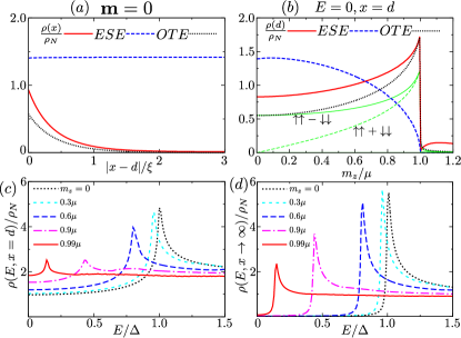
Figure 2: (a) Evolution of $\rho(E=0)$, angle-averaged $|F_{0}|$, and $F_{t}$ with the distance inside the superconducting region from the interface at $x=d$ at zero magnetization and $E=0$. (b) Same quantities as before as a function of $m_{z}$, for $E=0$ and $x=d$. The green solid and dashed lines correspond to the two triplet polarizations $|F_{1,2}|\propto(\uparrow\uparrow\mp\downarrow\downarrow)$, respectively. (c,d) LDOS as a function of the energy for several values of $m_{z}$ calculated at the IS interface $x=d$ (c), and inside the superconducting region, where $x\rightarrow\infty$ (d). For all plots, we set $\mu_{N}=10\mu$, $\mu_{I}=20\mu$, $\mu_{S}=\mu=10^{3}\Delta$, and $d=0.1(v_{F}/\mu)$.

We show in Fig. 2(a) the evolution of the angle-averaged quantities $|F_{0}(E=0)|$ and $F_{t}(E=0)$ as a function of the distance inside the superconducting region (dashed blue and dotted black lines, respectively). The bulk ESE contribution is dominant and responsible for the suppression of the density of states (red solid line) for $x>\xi$. At the interface, however, we find that $F_{t}(E=0)\neq 0$. The OTE contribution vanishes inside the superconducting region but is responsible for the enhancement of the LDOS close to the interface.

III.2 Symmetry analysis for out-of-plane effective magnetization

We now study the local anomalous Green function for an out-of-plane effective magnetization. We present a list of the components of the anomalous Green function in Appendix D, for the perpendicular case treated here and for the in-plane one analyzed in the next section. The presence of the perpendicular magnetization affects all components and, in particular, induces two new bulk terms. $F_{1,\infty}$ is proportional to $k_{y}=|k|\sin\theta$ (ETO) and becomes zero after integration over $\theta$. On the other hand, $F_{3,\infty}$ is an OTE term proportional to $Em_{z}$ and it vanishes in the absence of magnetization or for $E=0$. Therefore, the main effect on the bulk region is determined by $F_{0}$.

The situation is different at the interface. We plot in Fig. 2(b) angle-averaged $|F_{0}(E=0)|$ and $F_{t}(E=0)$ (blue dashed and black dotted lines, respectively), as a function of $m_{z}$, for $x=d$. We choose $E=0$ to analyze the symmetry of any zero-energy peak in the LDOS (red solid line). The edge contributions of the triplet components have odd-frequency parts that remain finite after integrating over the incident angles. $F_{t}(0)$ becomes comparable to $|F_{0}(0)|$ for a magnetization strength $m_{z}\approx 0.7\mu$. Additionally, we plot the triplet components $|F_{1,2}(E=0)|\propto(\uparrow\uparrow\mp\downarrow\downarrow)$ using solid and dashed green lines, respectively. At $m_{z}=0$, only $|F_{1}(0)|$ is present. For a finite $m_{z}$, $|F_{2}(0)|$ becomes a finite OTE term and increases with the field strength like $|F_{1}|$ at the same rate that the ESE term is suppressed. The LDOS at the interface is enhanced accordingly. With the increase of $m_{z}$, the feature of a Majorana resonant state becomes more pronounced. Also, here Majorana resonances are always accompanied by odd-frequency pairing.

The magnetization reduces the bulk gap $\Delta_{z}$, given in Eq. (7), for $m_{z}\leq\mu$. After the gap closes, the LDOS and the anomalous terms of the Green function are strongly suppressed. We show the energy dependence of the LDOS at the interface with $x=d$ in Fig. 2(c) and in the bulk of the superconducting region with $x\rightarrow\infty$ in Fig. 2(d). At the interface, the LDOS features a strong resonance at $|E|=\Delta_{z}$ and is finite for $|E|<\Delta_{z}$. For $m_{z}>\mu$, the LDOS is still finite and maximum at $E=0$ [see Fig. 2(b)]. However, the value of this finite LDOS at the interface decreases rapidly when increasing $m_{z}$ over $\mu$ because it is suppressed by a magnetic gap. Deep inside the superconducting region, where only the ESE component of the anomalous Green function is finite, we find a BCS-type density of states around the effective gap $\Delta_{z}$. For $m_{z}>\mu$, a magnetic gap opens destroying superconductivity.

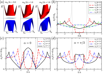
Figure 3: (a) Energy-momentum plot of the low-energy bands inside the superconducting region for several values of $m_{\parallel}$. (b) Bulk LDOS of the superconducting region of the NIS junction as a function of the excitation energy $E$ for different $m_{\parallel}$. (c,d) LDOS at the interface $x=d$ with $\mu_{I}/\mu=10$ and $d=0.1(v_{F}/\mu)$ as a function of the excitation energy $E$ with different in-plane magnetizations. We show $\alpha/\pi=0,0.5$ for (c,d), respectively. For (b,c,d) we set $\mu=10^{3}\Delta$.

III.3 Symmetry analysis for in-plane effective magnetization

In the previous section, we showed that the effect of a magnetic field in the heavily-doped, weak-field approximation is a Doppler-type shift of the excitation energy. This shift has an important effect on the energy bands: in Fig. 3(a), we plot the conduction (red) and valence (blue) bands in momentum space for several values of $m_{\parallel}$. For reference, the zero-energy plane is marked by a gray area. At zero field, the spectrum has rotational symmetry and the superconducting gap is the same for $|\mathbf{k}|=k_{F}$. For finite fields, $m_{\parallel}\neq 0$, the rotational symmetry of the spectrum is broken. However, particle-hole symmetry is recovered using $\epsilon(\mathbf{k})=-\epsilon(-\mathbf{k})$. The orientation of the NIS interfaces with respect to this bulk spectrum becomes very important since the energy spectrum can be asymmetric around $k_{y}=0$, with $k_{y}$ the momentum component parallel to the interface. Only the case where the in-plane field is oriented parallel to the normal-superconductor interface, i.e., for $\alpha=\pi/2$, the energy bands are $k_{y}$-symmetric. Additionally, there is a critical magnetization $m_{\parallel}=\Delta$ where both bands touch the zero-energy plane and the superconducting gap closes at some values of $|\mathbf{k}|=k_{F}$, for any orientation of the in-plane field. The orientation of the in-plane field $\alpha$ changes the position in momentum space where this closing occurs [Thegapclosingcangreatlyaffecttheedgestatesofthetwo-dimensionalTI; asrecentlydescribedin][]Reinthaler_2015.

To study the effect of the gap closing on the bulk of the superconducting region, we show the bulk density of states in Fig. 3(b) for several values of $m_{\parallel}$. After averaging over the angle of incidence, the bulk density of states is independent of the orientation of the magnetization. When $0<m_{\parallel}<\Delta$, the effective gaps $\Delta_{\pm}$ defined in Eq. (9) emerge and the LDOS exhibits a peak at $E\sim|\Delta_{+}|$ and is gapped for $E\lesssim|\Delta_{-}|$. When the gap closes for $m_{\parallel}=\Delta$, the bulk density of states becomes V-shaped with two resonances at $E=\pm 2\Delta$. For this case, the LDOS at the interface features a sharp zero-energy peak for any orientation of the in-plane field, as it is shown in the dashed-dotted blue lines of Fig. 3(c,d). Beyond this point, the zero-energy peak becomes wider if $\alpha<\pi/4$ or splits into two otherwise. For the bulk LDOS, a region emerges around $E=0$ with a flat density of states of the same magnitude as that of the normal region. Outside this energy range, the V-shaped profile becomes wider with increasing the strength of the field.

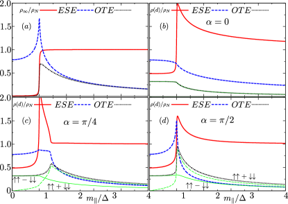
Figure 4: Plots of $\rho(E=0)$, $|F_{0}(E=0)|$, and $F_{t}(E=0)$ as a function of $m_{\parallel}$. (a) Bulk results for $x\rightarrow\infty$. (b,c,d) Results at the interface with $x=d$ for different orientations of the effective magnetization: $\alpha/\pi=0,0.25,0.5$ for (b,c,d), respectively. The solid and dashed green lines correspond to the polarizations $\uparrow\uparrow-\downarrow\downarrow$ and $\uparrow\uparrow+\downarrow\downarrow$ of the OTE term, respectively. For all plots, $\mu_{N}=\mu_{S}=\mu=10^{3}\Delta$, $\mu_{I}/\mu=10$, and $d=0.1(v_{F}/\mu)$.

We now study the components of the anomalous Green function plotting the bulk contribution of $|F_{0}(E=0)|$ and $F_{t}(0)$ as a function of $m_{\parallel}$ in Fig. 4(a). There are two distinct regimes. For $m_{\parallel}<\Delta$, the ESE term is greatly enhanced, while the OTE is finite but small compared to it. The LDOS is suppressed which corresponds to a conventional gapped profile. For the critical magnetization $m_{\parallel}=\Delta$, all terms increase. At this point, the LDOS jumps from $0$ to $1$. From then on, the triplet vector magnitude is finite and similar to the ESE term for $m_{\parallel}\gtrsim 2\Delta$ while the LDOS remains constant. Therefore, a finite bulk LDOS is obtained because of an equal superposition of OTE and ESE terms in the bulk of the superconducting region.

We show in Fig. 4(b,c,d) the ESE and OTE components at the interface ($x=d$), as a function of $m_{\parallel}$ for different orientations of the in-plane magnetization [$\alpha=0$, $\pi/4$, and $\pi/2$ for Figs. 4(b), 4(c), and 4(d), respectively]. For the symmetric orientation $\alpha=\pi/2$, the OTE term becomes dominant over the singlet one for values equal or greater than the critical magnetization [Fig. 4(d)]. In the opposite case with $\alpha=0$ [Fig. 4(b)], the singlet term is always dominant over the triplet one. Independently of the orientation, the LDOS is greatly enhanced for values greater than the critical one.

Finally, the behavior of $|F_{1,2}|\propto(\uparrow\uparrow\mp\downarrow\downarrow)$ strongly depends on the orientation of the magnetization (see green solid and dashed lines for $|F_{1,2}|$, respectively). Indeed, for $\alpha=0$ we find that $|F_{1}|=|F_{2}|$ while they are very different for $\alpha\neq 0$. Therefore, the spin polarization of the induced Cooper pairs can be controlled by the orientation of the external field .

IV Conductance spectroscopy

Our setup, sketched in Fig. 1, is ideal for conductance spectroscopy measurements like the ones recently performed in Refs. Finck et al., 2014; Snelder et al., 2015b. The conductance of the NIS junction, obtained from Eq. (20), is normalized to $G_{0}=G_{NS}(E\gg\Delta)$, as it is commonly done in experiments.

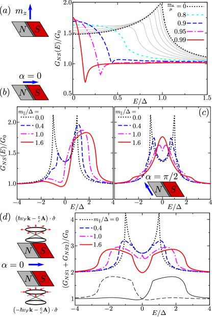
Figure 5: Conductance as a function of the excitation energy for several effective magnetizations. For each case we include a sketch of the NIS junction displaying the orientation of the effective magnetization as a blue arrow. (a) A perpendicular magnetization is finite in the whole NIS junction with $\mu_{N}=10\mu$, $\mu_{I}=20\mu$, and $\mu_{S}=\mu$. The thin gray lines are taken at intervals $0.1\mu$ from $m_{z}=0$. (b,c) In-plane magnetization finite in the whole junction oriented perpendicular (b) or parallel (c) to the NIS interfaces. For both cases, $\mu_{N}=\mu_{S}=\mu$ and $\mu_{I}/\mu=10$. (d) With the same parameters as (b), superposition of the conductance for both surfaces; sketched on the left. The black solid line corresponds to the $m_{\parallel}/\Delta=1.6$ case of (b) while the dashed one is the conductance of the other surface with the same parameters. In all plots, $d=0.1(v_{F}/\mu)$ and $\mu=10^{3}\Delta$.

We start considering an out-of-plane effective magnetization finite in the whole junction. Consequently, when we approach the critical point where $m_{z}\sim\mu$, a magnetic gap starts to develop in both normal and superconducting regions. In order to have propagating states in the normal region, we choose $\mu_{N}=10\mu$ and $\mu_{S}=\mu=10^{3}\Delta$. We still include a square potential barrier setting $\mu_{I}=20\mu$. The results for this setup are shown in Fig. 5(a) for several values of $m_{z}$ in the range $0<m_{z}<\mu$. For $m_{z}=0$, the tunnel conductance features a gapped profile. Due to the Klein tunneling effect, the conductance is not fully gapped for $E<\Delta$, even in the presence of a strong barrier. For $0<m_{z}<\mu$, the effective gap is reduced and, as $m_{z}$ approaches $\mu$, the subgap conductance increases clearly featuring a zero-bias peak. The formation of this zero-bias peak coincides with the regime where the odd-frequency triplet $F_{t}$ becomes dominant with respect to the ESE term $|F_{0}|$ [see Fig. 2(b)]. For $m_{z}>\mu$, the gap in the excitation spectrum is given by $E_{z}=|m_{z}-\sqrt{\mu^{2}+\Delta^{2}}|$ and the conductance is zero for $|E|\leq E_{z}$.

We now consider an in-plane magnetization in the heavily-doped, weak-field approximation. Under this approximation, if we take $\mu_{N}\sim\mu_{S}\gg|E|,\Delta,m_{\parallel}$, the effect of the field in the normal and intermediate regions is almost negligible. Assuming a setup with a symmetric square potential barrier with $\mu_{N}=\mu_{S}=\mu$ and $\mu_{I}=10\mu$, we plot in Fig. 5(b,c) the conductance for several values of $m_{\parallel}$. We show an in-plane magnetization perpendicular to the NIS interfaces ($\alpha=0$) in Fig. 5(b) and parallel to them ($\alpha=\pi/2$) in Fig. 5(c). In both cases, the effect of the field is to split the superconducting gap into two effective gaps $\Delta_{\pm}$ defined in Eq. (9).

For $\alpha=\pi/2$, the resonance at $E=\Delta$ for $m_{\parallel}=0$ remains pinned to the smallest of the gaps, but the one at the biggest gap is smeared by the angle average. Due to Klein tunneling, these resonances can not be clearly resolved in the conductance, although they appear in the LDOS, as shown in Fig. 3(c,d). The smallest of the gaps closes for $m_{\parallel}\gtrsim\Delta$ and a zero-energy peak appears in the conductance. It is in this regime where the odd-frequency triplet term is greater than the singlet one, as shown in Fig. 4(d).

Strikingly, for $\alpha\neq\pi/2$, the conductance is asymmetric with the energy. This asymmetry is a consequence of the distortion of the energy bands by the magnetic field, as shown in Fig. 3(a). The field breaks the rotation symmetry of the energy bands and the modified bands have a point-like symmetry that is determined by the orientation of the in-plane magnetization. Since we study transport in the direction perpendicular to the NIS interfaces, when the magnetization is aligned with the interface, i.e., $\alpha=\pi/2$, the symmetry is recovered [see Fig. 5(c)], while it is lost for any other orientation.

Owing to the special particle-hole symmetry of our system, we find that, for $\alpha\neq\pi/2$, Andreev reflection is very asymmetric with the energy while normal reflection is symmetric. This effect holds independently of the barrier strength provided that the effective magnetization is misaligned with the NIS interface. Thus, as an example, we can consider a junction with $\mu_{I}=\mu_{S}\neq\mu_{N}$. For such junctions, normal and Andreev reflections take place separately at each side of the intermediate region. In the setup of Fig. 1(a), when $|E|\leq\Delta$, normal (Andreev) reflection is the only scattering process at $x=0$ ($x=d$). The reflection amplitudes are then

$$a_{1}(E,\theta)={} \frac{2\cos\theta_{N}\cos\theta_{S}}{t(E,\theta)}\Gamma_{-}\quad,$$ (23a)

$$b_{1}(E,\theta)={} i\frac{\sin\theta_{N}-\sin\theta_{S}}{t(E,\theta)}\left(1-\Gamma_{+}\Gamma_{-}\right)\quad,$$ (23b)

$$t(E,\theta)={} 1+\cos\left(\theta_{N}+\theta_{S}\right)$$

$$-\Gamma_{+}\Gamma_{-}\left[1-\cos\left(\theta_{N}-\theta_{S}\right)\right]\quad,$$

with $\theta_{N,S}=\sin^{-1}(k_{y}/\mu_{N,S})$ and

$$\Gamma_{\pm}={} \frac{\Delta^{*}}{\epsilon_{\pm}+\sqrt{(\epsilon_{\pm})^{2}-|\Delta|^{2}}}\quad,$$

$$\epsilon_{\pm}={} E\pm m_{\parallel}\cos(\theta_{S}-\alpha)\quad.$$

Due to the spin-momentum locking at the surface of the 3DTI, the magnetic field affects differently quasiparticles moving in opposite directions Reinthaler et al. (2015). That is the reason why Andreev reflection is asymmetric with the magnetization, being proportional to $\Gamma_{-}$ while normal reflection is not, since it goes with $(1-\Gamma_{+}\Gamma_{-})$. As a consequence, the conductance becomes more asymmetric as we increase $m_{\parallel}$, as shown in Fig. 5(b). The energy range where Andreev reflection is enhanced also becomes wider. In the figure, this happens always for positive energies.

Finally, the asymmetry in the conductance is also partly a consequence of having limited our analysis of transport to only one surface of the 3DTI. In Eq. (1), the Dirac Hamiltonian chosen to describe electron-like quasiparticles is $\hat{h}(\mathbf{k})=[v_{F}\mathbf{k}-e\mathbf{A}]\cdot\hat{\sigma}$. With this choice, quasi-particles have positive helicity, i.e., their spin points in the direction of their momentum. For the opposite surface state of the 3DTI, however, electron-like quasiparticles are described by $\hat{h}(\mathbf{k})=[-v_{F}\mathbf{k}-e\mathbf{A}]\cdot\hat{\sigma}$. Therefore, the sign of their helicity changes and their spin points in the opposite direction of their momentum. As a consequence, the effect of the in-plane magnetization is reversed, with $\Gamma_{\pm}\rightarrow\Gamma_{\mp}$. The normal reflection amplitude is unchanged, but the Andreev reflection amplitude becomes proportional to $\Gamma_{+}$ in Eq. (23). The asymmetry of the conductance is reversed, as it is shown by the black solid and dashed lines of Fig. 5(d), corresponding to the $m_{\parallel}/\Delta=1.6$ case of Fig. 5(b). If we consider a conductance measurement that includes opposite surfaces of the 3DTI, the symmetry with the energy is recovered. For the same parameters as Fig. 5(b), we show such conductance spectroscopy in Fig. 5(d).

V Conclusions

We have analyzed the superconducting proximity effect at 3DTI-superconductor hybrids in the presence of an effective magnetization. We find that the interplay between the magnetization and the spin-momentum locking of the surface state gives rise to interesting odd-frequency triplet terms in the induced pair potential. Contrary to the usual even-frequency triplet terms, averaging over the angle of incidence does not cancel these components, and their effect can be observed in experimental transport observables such as the NIS conductance and LDOS.

For an out-of-plane magnetization, the OTE terms increase with the strength of the field in the regime $\mu>m_{z}>0$. At the same time, the singlet term of the induced pair potential is suppressed. As a consequence, the conductance evolves from a conventional gapped profile for $m_{z}=0$ into a zero-bias conductance peak when $m_{z}\lesssim\mu$. Such strong magnetization can be induced in the system when a ferromagnetic insulator such as EuS is deposited on top of the NIS junction Wei et al. (2013), in a setup like the one sketched in Fig. 1(b).

If we consider the effect of an orbital magnetic field on the junction, we find a similar gap to zero-energy peak transition on the conductance for in-plane magnetization parallel to the NIS interface. The main difference is that the critical value that determines the emergence of a zero-energy peak is now $m_{\parallel}=\Delta$, where the energy bands feature an indirect closing of the gap. For $m_{\parallel}\geq\Delta$, the OTE term is greater than the ESE one at the interface and similar in magnitude in the bulk superconducting region. As a result, we have connected the emergence of odd-frequency triplet in the induced pair potential on the surface of the 3DTI with a distinctive profile of the conductance.

When the in-plane magnetization is not oriented parallel to the interface, the conductance becomes asymmetric with the energy. This is a manifestation of the breaking of the rotational symmetry of the band structure of the combined 3DTI-superconductor system. Only a transport measurement that probes one surface state of the 3DTI can detect the asymmetry of the conductance. Such setup, would be a perfect platform to probe the coexistence of topological order and superconductivity.

Our results show that 3DTI-based NIS junctions feature a very rich induced superconducting pair potential that displays the elusive odd-frequency triplet component. Using very basic ingredients such as a conventional superconductor and an external magnetic field or ferromagnetic insulator, standard experimental techniques like conductance spectroscopy can be used to detect signatures of OTE superconductivity.

Appendix A Scattering states

In this appendix, we present the solutions of the BdG equations $\check{H}\Psi=E\Psi$, for the two orientations of the effective magnetization considered in the main text. In the normal regions with $\Delta=0$, the general solution of the BdG equations is

$$\Psi(x<d)={} A_{N}^{+}\psi_{+k_{e}}\mathrm{e}^{ik_{e}x}+A_{N}^{-}\psi_{-k_{e}}\mathrm{e}^{-ik_{e}x}$$

$$+ B_{N}^{+}\psi_{+k_{h}}\mathrm{e}^{ik_{h}x}+B_{N}^{-}\psi_{-k_{h}}\mathrm{e}^{-ik_{h}x}\quad,$$ (24)

where the coefficients $A_{N}^{\pm}$ ($B_{N}^{\mp}$) represent the amplitudes for electrons (holes) propagating to the right and left, respectively.

On the other hand, for the superconducting region we find

$$\Psi(x>d)={} A_{S}^{+}\psi_{+k_{1}}\mathrm{e}^{ik_{1}x}+A_{S}^{-}\psi_{-k_{1}}\mathrm{e}^{-ik_{1}x}$$

$$+ B_{S}^{+}\psi_{+k_{2}}\mathrm{e}^{ik_{2}x}+B_{S}^{-}\psi_{-k_{2}}\mathrm{e}^{-ik_{2}x}\quad,$$ (25)

where the coefficients $A_{S}^{\pm}$ ($B_{S}^{\mp}$) now label the amplitudes for right and left moving electron-like (holes-like) quasiparticles.

A.1 Junctions with out-of-plane effective magnetization

In the normal state regions with $\Delta=0$, the wave vector is given by $k_{e,h}=\sqrt{Z_{e+}Z_{e-}-(v_{F}k_{y})^{2}}/(v_{F})$, with $Z_{e\pm}=\mu+E\pm m_{z}$ and $Z_{h\pm}=\mu-E\pm m_{z}$. The wave functions in Eq. (24) are then given by

$$\psi_{\pm k_{e}}={} \left[1,\pm\mathrm{e}^{\pm i\theta_{e}},0,0\right]^{T}\quad,$$ (26a)

$$\psi_{\pm k_{h}}={} \left[0,0,1,\mp s_{h}\mathrm{e}^{\pm i\theta_{h}}\right]^{T}\quad,$$ (26b)

where we have defined the phase factors

$$\mathrm{e}^{\pm i\theta_{e}}=v_{F}\frac{k_{e}\pm ik_{y}}{|Z_{e+}|}\quad,\quad\mathrm{e}^{\pm i\theta_{h}}=v_{F}\frac{k_{h}\pm s_{h}ik_{y}}{|Z_{h-}|}\quad,$$

and $s_{h}=\operatorname{sgn}(\mu-E)$.

Analogously, for the superconducting region, the wave vectors are given by $k_{j}=\sqrt{Z_{j+}Z_{j-}-(v_{F}k_{y})^{2}}/(v_{F})$, with $j=1,2$,

$$Z_{1(2)\pm}={} \frac{\mu^{2}-m_{z}^{2}+(-)\mu\Omega_{z}\pm Em_{z}}{\mu\pm m_{z}}\quad,$$

$$\Omega_{z}={} \left\{\begin{array}[]{cl}\operatorname{sgn}\left(E\right)\sqrt{E^{2}-\Delta_{z}^{2}}&,|E|>\Delta_{z}\\ i\sqrt{\Delta_{z}^{2}-E^{2}}&,|E|\leq\Delta_{z}\end{array}\right.\quad,$$

and $\Delta_{z}=\Delta\sqrt{1-(m_{z}/\mu)^{2}}$. The corresponding wave functions in Eq. (25) are

$$\psi_{\pm k_{1}}={} \left[\Gamma_{1},\pm E_{1\pm}\Gamma_{1},\mp\zeta E_{1\pm},1\right]^{T}\quad,$$ (27a)

$$\psi_{\pm k_{2}}={} \left[\Gamma_{2},\pm E_{2\pm}\Gamma_{2},\mp\zeta E_{2\pm},1\right]^{T}\quad,$$ (27b)

with

$$E_{1(2)\pm}={} \frac{Z_{1(2)+}}{v_{F}(k_{1(2)}\mp ik_{y})}\quad,$$

$$\Gamma_{1,2}={} \frac{\mu E\pm\mu\Omega_{z}}{\Delta(\mu-m_{z})}\quad,$$

$$\zeta={} \Gamma_{1}\Gamma_{2}=\frac{\mu+m_{z}}{\mu-m_{z}}\quad.$$

A.2 Junctions with in-plane effective magnetization

In the normal region, where $\Delta=0$, the wave vector component perpendicular to the interface becomes $k^{\lessgtr}_{e,h}=k_{e,h}\!\pm\!m_{x}/v_{F}$ with $v_{F}k_{e,h}\!=\!\sqrt{\left(\mu\pm E\right)^{2}\!-\!\left(v_{F}k_{y}\pm m_{y}\right)^{2}}$. The superscript $>$ ($<$) labels right (left) movers along the $x$-direction. Electrons and holes have an opposite shift by the field. When they are coupled by the superconductor, this shift becomes very important. Therefore, the component of the in-plane magnetization perpendicular to the interface, $m_{x}=m_{\parallel}\cos\alpha$, discriminates between particles that move with or against the stream of Cooper pairs. The general solution of the BdG equations for the normal state region is given in Eq. (24) with the same wave functions defined in Eq. (26), but the new phase factors

$$\mathrm{e}^{i\theta_{e,h}}=\frac{v_{F}k_{e,h}+i\left(v_{F}k_{y}\pm m_{y}\right)}{|\mu\pm E|}\quad.$$

In the heavily-doped regime $\mu\gg E,\Delta$, we have $\theta=\sin^{-1}\left(k_{y}/\mu\right)$, $k_{1,2}\sim k_{Fx}\pm i\kappa_{2}$, and $-k_{1,2}\sim-k_{Fx}\mp i\kappa_{1}$, with

$$\kappa_{1,2}=\frac{\sqrt{|\Delta|^{2}-(E\pm\mathbf{n}\cdot\mathbf{m})^{2}}}{v_{F}\cos\theta}\quad,$$

and $k_{Fx}=k_{F}\cos\theta$. Under this approximation, the wave functions in Eq. (25) are

$$\psi_{\pm k_{1}}={} \left[1,\pm\mathrm{e}^{\pm i\theta},\mp\Gamma_{\mp}\mathrm{e}^{\pm i\theta},\Gamma_{\mp}\right]^{T}\quad,$$ (28a)

$$\psi_{\pm k_{2}}={} \left[\Gamma_{\mp},\pm\Gamma_{\mp}\mathrm{e}^{\pm i\theta},\mp\mathrm{e}^{\pm i\theta},1\right]^{T}\quad.$$ (28b)

with

$$\Gamma_{\pm}=\frac{\Delta^{*}}{(E\pm\mathbf{n}\cdot\mathbf{m})+\sqrt{(E\pm\mathbf{n}\cdot\mathbf{m})^{2}-|\Delta|^{2}}}\quad.$$

Appendix B Green function techniques for Dirac systems

For an incoming electron from the normal region, the wave function is

$$\Psi_{1}(x)\!\!=\!\!\left\{\!\!\begin{array}[]{lr}\begin{array}[]{c}\mathrm{e}^{ik_{e}x}\psi_{+k_{e}}\!+\!a_{1}\mathrm{e}^{ik_{h}x}\psi_{+k_{h}}\\ +b_{1}\mathrm{e}^{-ik_{e}x}\psi_{-k_{e}}\end{array}\,,&x<0\\ c_{1}\mathrm{e}^{ik_{1}x}\psi_{+k_{1}}\!+\!d_{1}\mathrm{e}^{-ik_{2}x}\psi_{-k_{2}}\,,&x>d\end{array}\right.\,.$$ (29)

For the other processes, we find

$$\Psi_{2}(x)\!\!=\!\!\left\{\!\!\begin{array}[]{lr}\begin{array}[]{c}\mathrm{e}^{-ik_{h}x}\psi_{-k_{h}}\!+\!a_{2}\mathrm{e}^{-ik_{e}x}\psi_{-k_{e}}\\ +b_{2}\mathrm{e}^{ik_{h}x}\psi_{+k_{h}}\end{array}\,,&x<0\\ c_{2}\mathrm{e}^{-ik_{2}x}\psi_{-k_{2}}\!+\!d_{2}\mathrm{e}^{ik_{1}x}\psi_{+k_{1}}\,,&x>d\end{array}\right.\,,$$ (30)

$$\Psi_{3}(x)\!\!=\!\!\left\{\!\!\begin{array}[]{lr}c_{3}\mathrm{e}^{-ik_{e}x}\psi_{-k_{e}}\!+\!d_{3}\mathrm{e}^{ik_{h}x}\psi_{+k_{h}}\,,&x<0\\ \begin{array}[]{c}\mathrm{e}^{-ik_{1}x}\psi_{-k_{1}}\!+\!a_{3}\mathrm{e}^{-ik_{2}x}\psi_{-k_{2}}\\ +b_{3}\mathrm{e}^{ik_{1}x}\psi_{+k_{1}}\end{array}\,,&x>d\end{array}\right.\,,$$ (31)

and,

$$\Psi_{4}(x)\!\!=\!\!\left\{\!\!\begin{array}[]{lr}c_{4}\mathrm{e}^{ik_{h}x}\psi_{+k_{h}}\!+\!d_{3}\mathrm{e}^{-ik_{e}x}\psi_{-k_{e}}\,,&x<0\\ \begin{array}[]{c}\mathrm{e}^{ik_{2}x}\psi_{+k_{2}}\!+\!a_{4}\mathrm{e}^{ik_{1}x}\psi_{+k_{1}}\\ +b_{4}\mathrm{e}^{-ik_{2}x}\psi_{-k_{2}}\end{array}\,,&x>d\end{array}\right.\,.$$ (32)

At the intermediate region, we use the wave functions

$$\Psi_{j}(0<x<d)={} p_{j}\mathrm{e}^{ik_{e}^{I}x}\psi_{+k_{e}^{I}}^{I}\!+\!q_{j}\mathrm{e}^{-ik_{e}^{I}x}\psi_{-k_{e}^{I}}^{I}$$ (33)

$$+r_{j}\mathrm{e}^{-ik_{h}^{I}x}\psi_{-k_{h}^{I}}^{I}\!+\!s_{j}\mathrm{e}^{ik_{h}^{I}x}\psi_{+k_{h}^{I}}^{I}\quad,$$

which correspond to the normal region solutions with the change $\mu\rightarrow\mu_{I}$ and where $j=1,\dots,4$ labels the processes.

The corresponding reflection and transmission amplitudes are obtained inserting Eqs. (26), (27), and (28) into the boundary conditions

$$\Psi_{j}(0^{-})=\Psi_{j}(0^{+})\quad,\quad\Psi_{j}(d-0^{+})=\Psi_{j}(d+0^{+})\quad.$$ (34)

Next, we insert the resulting wave functions for the scattering processes in the retarded Green function defined in Eq. (10). The wave functions $\tilde{\Psi}_{i}(x)$ correspond to the conjugate scattering processes to $\Psi_{i}(x)$ and are solutions of $\check{H}^{*}(\mathbf{k})$ with the change $\mathbf{k}\rightarrow-\mathbf{k}$. The conjugated wave vectors are obtained by the transformation

$$\tilde{\psi}_{\pm k_{x}}(k_{y})=\psi_{\mp k_{x}}(-k_{y})\quad,$$

which is a parity transformation.

We now consider the Green function of the normal region, imposing that $k_{e,h}>0$. We substitute the solutions with $x<0$ of Eqs. (29), (30), (31), and (32) into Eq. (10) and apply the continuity condition of Eq. (18) to obtain

$$G^{r}(x,x^{\prime})=\frac{i}{2v_{F}}$$

$$\times\left\{\!\!\begin{array}[]{lr}\left(\!\!\begin{array}[]{cc}\frac{\mathrm{e}^{ik_{e}|x-x^{\prime}|}}{\cos\theta_{e}}\psi_{-k_{e}}\psi_{-k_{e}}^{\dagger}+b_{1}\frac{\mathrm{e}^{-ik_{e}(x+x^{\prime})}}{\cos\theta_{e}}\psi_{-k_{e}}\psi_{+k_{e}}^{\dagger}&a_{1}\frac{\mathrm{e}^{-i(k_{e}x-k_{h}x^{\prime})}}{\cos\theta_{e}}\psi_{-k_{e}}\psi_{-k_{h}}^{\dagger}\\ a_{2}\frac{\mathrm{e}^{-i(k_{e}x^{\prime}-k_{h}x)}}{\cos\theta_{h}}\psi_{+k_{h}}\psi_{+k_{e}}^{\dagger}&\frac{\mathrm{e}^{-ik_{h}|x-x^{\prime}|}}{\cos\theta_{h}}\psi_{-k_{h}}\psi_{-k_{h}}^{\dagger}+b_{2}\frac{\mathrm{e}^{ik_{h}(x+x^{\prime})}}{\cos\theta_{h}}\psi_{+k_{h}}\psi_{-k_{h}}^{\dagger}\end{array}\!\!\right)\,\,,&0>x^{\prime}>x\\ \left(\!\!\begin{array}[]{cc}\frac{\mathrm{e}^{ik_{e}|x-x^{\prime}|}}{\cos\theta_{e}}\psi_{+k_{e}}\psi_{+k_{e}}^{\dagger}+b_{1}\frac{\mathrm{e}^{-ik_{e}(x+x^{\prime})}}{\cos\theta_{e}}\psi_{-k_{e}}\psi_{+k_{e}}^{\dagger}&a_{2}\frac{\mathrm{e}^{-i(k_{e}x-k_{h}x^{\prime})}}{\cos\theta_{h}}\psi_{-k_{e}}\psi_{-k_{h}}^{\dagger}\\ a_{1}\frac{\mathrm{e}^{-i(k_{e}x^{\prime}-k_{h}x)}}{\cos\theta_{e}}\psi_{+k_{h}}\psi_{+k_{e}}^{\dagger}&\frac{\mathrm{e}^{-ik_{h}|x-x^{\prime}|}}{\cos\theta_{h}}\psi_{-k_{h}}\psi_{-k_{h}}^{\dagger}+b_{2}\frac{\mathrm{e}^{ik_{h}(x+x^{\prime})}}{\cos\theta_{h}}\psi_{+k_{h}}\psi_{-k_{h}}^{\dagger}\end{array}\!\!\right)\,\,,&0>x>x^{\prime}\end{array}\right.\quad.$$ (41)

Finally, the Green function on the superconducting side of the junction, with $\operatorname{Re}\left\{k_{1,2}\right\}>0$, is

$$G^{r}(x,x^{\prime})=$$

$$\left\{\begin{array}[]{cr}\begin{array}[]{c}A_{1}\left[\mathrm{e}^{ik_{1}(x^{\prime}-x)}\psi_{-k_{1}}\tilde{\psi}_{+k_{1}}^{T}+a_{3}\mathrm{e}^{i(k_{1}x^{\prime}-k_{2}x)}\psi_{-k_{2}}\tilde{\psi}_{+k_{1}}^{T}+b_{3}\mathrm{e}^{ik_{1}(x^{\prime}+x)}\psi_{+k_{1}}\tilde{\psi}_{+k_{1}}^{T}\right]\\ +A_{2}\left[\mathrm{e}^{-ik_{2}(x^{\prime}-x)}\psi_{+k_{2}}\tilde{\psi}_{-k_{2}}^{T}+a_{4}\mathrm{e}^{-i(k_{2}x^{\prime}-k_{1}x)}\psi_{+k_{1}}\tilde{\psi}_{-k_{2}}^{T}+b_{4}\mathrm{e}^{-ik_{2}(x^{\prime}+x)}\psi_{-k_{2}}\tilde{\psi}_{-k_{1}}^{T}\right]\end{array}&,x^{\prime}>x>d\\ \begin{array}[]{c}B_{1}\left[\mathrm{e}^{ik_{1}(x-x^{\prime})}\psi_{+k_{1}}\tilde{\psi}_{-k_{1}}^{T}+\tilde{a}_{3}\mathrm{e}^{i(k_{1}x-k_{2}x^{\prime})}\psi_{+k_{1}}\tilde{\psi}_{-k_{2}}^{T}+\tilde{b}_{3}\mathrm{e}^{ik_{1}(x+x^{\prime})}\psi_{+k_{1}}\tilde{\psi}_{+k_{1}}^{T}\right]\\ +B_{2}\left[\mathrm{e}^{-ik_{2}(x-x^{\prime})}\psi_{-k_{2}}\tilde{\psi}_{+k_{2}}^{T}+\tilde{a}_{4}\mathrm{e}^{-i(k_{2}x-k_{1}x^{\prime})}\psi_{-k_{2}}\tilde{\psi}_{+k_{1}}^{T}+\tilde{b}_{4}\mathrm{e}^{-ik_{2}(x+x^{\prime})}\psi_{-k_{2}}\tilde{\psi}_{-k_{2}}^{T}\right]\end{array}&,x>x^{\prime}>d\\ \end{array}\right.\quad,$$ (48)

where

$$A_{1}=B_{1}={} \frac{i}{v_{F}}\frac{Z_{1-}}{k_{1}}\frac{\Gamma_{1}^{-1}}{\Gamma_{1}-\Gamma_{2}}\quad,$$

$$A_{2}=B_{2}={} \frac{i}{v_{F}}\frac{Z_{2-}}{k_{2}}\frac{\Gamma_{2}^{-1}}{\Gamma_{1}-\Gamma_{2}}\quad,$$

for an out-of-plane magnetization and

$$A_{1}=B_{2}={} \frac{i}{v_{F}\cos\theta}\frac{1}{1-\Gamma_{+}^{2}}\quad,$$

$$A_{2}=B_{1}={} \frac{i}{v_{F}\cos\theta}\frac{1}{1-\Gamma_{-}^{2}}\quad,$$

for the in-plane magnetization in the heavily-doped, weak-field approximation ($\mu\gg\Delta,E,m_{\parallel}$) and with $|\theta|\leq\pi/2$. For the Green function with $\operatorname{Re}\left\{k_{1,2}\right\}<0$, the definition of the coefficients $A_{1,2}$ and $B_{1,2}$ changes sign. Consequently, the sign change in $1/k_{1,2}$ or, equivalently, $1/\cos\theta$ with $\pi/2<\theta<3\pi/2$, is canceled.

The Green function can be trivially separated into a bulk contribution, defined far away from the interface, and an edge term which contains the scattering at the interface. This is, $G^{r}(x,x^{\prime})\equiv G^{r}_{\infty}(x,x^{\prime})+G^{r}_{A}(x,x^{\prime})+G^{r}_{B}(x,x^{\prime})$, where we have divided the edge term into the part that is given by Andreev reflection processes [$G^{r}_{A}(x,x^{\prime})$] and the one that is given by normal reflections [$G^{r}_{B}(x,x^{\prime})$].

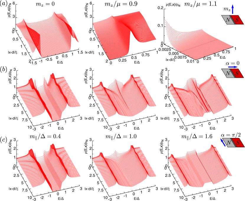
Figure 6: LDOS inside the superconducting region normalized to the bulk density of states in the normal region $\rho_{N}$ as a function of both the excitation energy and the distance from the interface ($x=d$). (a) Out-of-plane magnetization. From left to right, $m_{z}/\mu=0,0.9,1.1$. For the three panels, $\mu_{N}=10\mu$ and $\mu_{I}=20\mu$. (b) In-plane magnetization perpendicular to the NIS interface ($\alpha=0$). From left to right, $m_{\parallel}/\Delta=0.4,1.0,1.6$. (c) In-plane magnetization parallel to the NIS interface ($\alpha=\pi/2$). From left to right, $m_{\parallel}/\Delta=0.4,1.0,1.6$. For (b) and (c), $\mu_{N}=\mu$ and $\mu_{I}=10\mu$. For all plots, $\mu=10^{3}\Delta$ and $d=0.1(v_{F}/\mu)$.

Appendix C Local density of states

The electronic LDOS is obtained from the retarded Green function using Eq. (19). In the normal region is thus given by

$$\rho_{N}(E)\equiv\rho(E,x\rightarrow-\infty)$$

$$=-\frac{1}{\pi v_{F}}\int\limits_{-\pi/2}^{\pi/2}\mathrm{d}\theta\cos\theta\operatorname{Im}\left\{\frac{i}{\cos\theta_{e}}\right\}\quad,$$ (49)

for the bulk and

$$\rho_{B}(E,x)=-\frac{1}{\pi v_{F}}\int\limits_{\pi/2}^{\pi/2}\mathrm{d}\theta\cos\theta$$

$$\times\operatorname{Im}\left\{\tilde{b}_{1}(E,\theta)\tan\theta_{e}\mathrm{e}^{-i\theta_{e}}\mathrm{e}^{-2ik_{e}x}\right\}\quad,$$ (50)

for the edge. The LDOS in the normal region is thus $\rho(E,x<0)=\rho_{N}(E)+\rho_{B}(E,x)$.

Analogously, in the superconducting region we find, in the absence of magnetization,

$$\rho(E,x>d)=-\frac{1}{\pi v_{F}}\int\limits_{-\pi/2}^{\pi/2}\mathrm{d}\theta\cos\theta$$ (51)

$$\operatorname{Im}\left\{\frac{i\operatorname{sgn}\left(E\right)}{\cos\theta}\left(\frac{1+\Gamma^{2}}{1-\Gamma^{2}}+\frac{2\Gamma}{1-\Gamma^{2}}a_{3}\mathrm{e}^{-2\kappa x}\right)\right.$$

$$\left.+\frac{\tan\theta}{1-\Gamma^{2}}\left(\mathrm{e}^{i\theta}\mathrm{e}^{2ik_{1}x}b_{3}-\Gamma^{2}\mathrm{e}^{-i\theta}\mathrm{e}^{-2ik_{2}x}b_{4}\right)\right\}\quad.$$

We have neglected the rapidly oscillating terms proportional to the normal reflection amplitudes $b_{3,4}(E,\theta)$ in the edge contribution. The bulk contribution of Eq. (51) reduces to the BCS density of states $\rho(E,\mathbf{m}=0)=\operatorname{Re}\left\{E/\sqrt{E^{2}-\Delta^{2}}\right\}$. We plot in the left panel of Fig. 6(a) the LDOS for zero field as a function of the energy and the distance from the interface inside the superconducting region. The LDOS is finite for $|E|\leq\Delta$ at the interface ($x=d$) and decays to zero for distances inside the superconducting region comparable to the superconducting coherence length.

When we consider an in-plane magnetization, the previous result is changed to

$$\rho(E,x>d)=-\frac{1}{\pi v_{F}}\int\limits_{-\pi/2}^{\pi/2}\mathrm{d}\theta\cos\theta$$ (52)

$$\operatorname{Im}\left(\frac{i\operatorname{sgn}\left(E\right)}{\cos\theta}\left[\frac{1-\Gamma_{+}^{2}\Gamma_{-}^{2}}{(1-\Gamma_{+}^{2})(1-\Gamma_{-}^{2})}\right.\right.$$

$$\left.\left.+\left(\frac{\Gamma_{+}}{1-\Gamma_{+}^{2}}a_{3}+\frac{\Gamma_{-}}{1-\Gamma_{-}^{2}}a_{4}\right)\mathrm{e}^{-2\kappa x}\right]+\tan\theta\right.$$

$$\left.\times\left\{\begin{array}[]{lr}\frac{\mathrm{e}^{i\theta}b_{3}}{1-\Gamma_{+}^{2}}\mathrm{e}^{2ik_{1}x}-\frac{\Gamma_{+}\Gamma_{-}}{1-\Gamma_{-}^{2}}\mathrm{e}^{-i\theta}\mathrm{e}^{-2ik_{2}x}b_{4}&,E\geq 0\\ \frac{\mathrm{e}^{-i\theta}b_{3}}{1-\Gamma_{-}^{2}}\mathrm{e}^{2ik_{1}x}-\frac{\Gamma_{+}\Gamma_{-}}{1-\Gamma_{+}^{2}}\mathrm{e}^{i\theta}\mathrm{e}^{-2ik_{2}x}b_{4}&,E<0\end{array}\right.\right)\quad.$$ (55)

We plot in Fig. 6(b,c) the LDOS as a function of the energy and the distance from the IS interface at $x=d$ for several values of $m_{\parallel}$ and for $\alpha=0$ and $\alpha=\pi/2$, respectively. The effect of the in-plane magnetization is to split the superconducting gap into two, $\Delta\rightarrow\Delta_{\pm}$. When $m_{\parallel}<\Delta$, the LDOS at the interface clearly shows four resonances at $|E|=\Delta_{\pm}$ which become, inside the superconducting region, fully gapped for $|E|\leq\Delta_{-}$ with sharp resonances at $|E|=\Delta_{+}$ [see left panels of Fig. 6(b,c)]. For $m_{\parallel}=\Delta$, $\Delta_{-}=0$ and the LDOS inside the superconducting region adopts a V-shaped profile. At the interface, a peak at $E=0$ appears which has a long-range decay if $\alpha=0$ ($|x-d|\sim 10\xi$). For a magnetization oriented parallel to the interface ($\alpha=\pi/2$), the peak decays as $|x-d|\sim\xi$. This peak disappears when $m_{\parallel}>\Delta$ if $\alpha>\pi/4$, but it is still present and displays a long-range decay otherwise.

Finally, for an out-of-plane magnetization, the LDOS is given by

$$\rho(E,x>d)=-\frac{1}{\pi v_{F}}\int\mathrm{d}k_{y}\operatorname{Im}\left\{\operatorname{sgn}\left(E\right)\right.$$ (56)

$$\left.\times\left[A_{1}\Gamma_{1}^{2}(1+E_{1+}E_{1-})+A_{2}\Gamma_{2}^{2}(1+E_{2+}E_{2-})\right.\right.$$

$$\left.\left.+\Gamma_{1}\Gamma_{2}(A_{1}a_{2}+A_{2}a_{4})\mathrm{e}^{-2\kappa_{z}x}\right.\right.$$

$$\left.\left.\times\left\{\begin{array}[]{lr}1+E_{1+}E_{2-}&,E\geq 0\\ 1+E_{1-}E_{2+}&,E<0\end{array}\right\}\right.\right.$$ (59)

$$\left.\left.+A_{1}\Gamma_{1}^{2}(1-E_{1+}^{2})\mathrm{e}^{2ik_{1}x}b_{3}\right.\right.$$

$$\left.\left.-A_{2}\Gamma_{2}^{2}(1-E_{2-}^{2})\mathrm{e}^{-2ik_{2}x}b_{4}\right]\right\}\quad.$$

We show the LDOS results for a perpendicular magnetization close to the closing of the gap in the central and right panels of Fig. 6(a). Before the closing of the gap (central panel with $m_{z}=0.9$), the LDOS shows a resonance at the energies corresponding to the effective gap $\Delta_{z}$ and is greatly enhanced at zero energy close to the interface. This enhancement of the LDOS, however, decays fast inside the superconducting region and disappears at a distance comparable to the superconducting coherence length. After closing the gap (right panel with $m_{z}=1.1$), superconductivity is strongly suppressed and only a zero-energy peak on the LDOS survives at the interface. This peak decays inside the superconducting region within $10^{-2}\xi$.

Appendix D Anomalous Green function

We now analyze the electron-hole component in Nambu space of Eq. (48). For simplicity, we only consider NS junctions with no intermediate region. Moreover, we only show the case with $\operatorname{Re}\left\{k_{x}\right\}>0$. The symmetry classification remains the same for more complicated NIS junctions.

In the absence of magnetization, the Andreev reflection probabilities adopt the simple form $a_{3}=a_{4}=\tilde{a}_{3}=\tilde{a}_{4}=-\Gamma$ and the normal reflections are $b_{3}=b_{4}=\tilde{b}_{3}=\tilde{b}_{4}=0$. The components of the anomalous Green function are thus given by

$$F_{0}(E,\theta)\!={} \frac{i\operatorname{sgn}\left(E\right)}{2v_{F}\cos\theta}\left[\frac{2\Gamma}{1-\Gamma^{2}}+\frac{1+\Gamma^{2}}{1-\Gamma^{2}}a_{3}\mathrm{e}^{-2\kappa x}\right]\,,$$

$$F_{3}(E,\theta)\!={} 0\,,$$

$$F_{\uparrow\uparrow}(E,\theta)\!={} F_{\downarrow\downarrow}(E,\theta)$$

$$={} \frac{\operatorname{sgn}\left(E\right)}{2v_{F}\cos\theta}\left[\frac{2\Gamma}{1-\Gamma^{2}}+\frac{1+\Gamma^{2}}{1-\Gamma^{2}}a_{3}\mathrm{e}^{-2\kappa x}\right]\sin\theta$$

$$+\frac{i\tilde{\sigma}}{2v_{F}}a_{3}\mathrm{e}^{-2\kappa x}\quad,$$

with $\tilde{\sigma}=+1,-1$ for $F_{\uparrow\uparrow}$ and $F_{\downarrow\downarrow}$, respectively. We have defined $\Gamma=\Delta/(E+\Omega)$, $\kappa=-i\Omega/(v_{F}\cos\theta)$, and $\Omega=\sqrt{E^{2}-\Delta^{2}}$. The singlet term $F_{0}(E,\theta)$ is even in frequency and spatial dependence; therefore, it is classified as ESE. The first term of $F_{\sigma\sigma}(E,\theta)$, with $\sigma=\uparrow,\downarrow$, is equal to $F_{0}(E,\theta)$ multiplied by $\sin\theta$, which makes it even in energy but odd in spatial dependence, hence classified as ETO. The second term of $F_{\sigma\sigma}(E,\theta)$ is odd in energy and even in spatial dependence and is classified as OTE.

In the main text, we use the triplet components $F_{1,2}=F_{\uparrow\uparrow}\mp F_{\downarrow\downarrow}$. Due to the sign change for the edge part proportional to the Andreev reflection amplitude $a_{3}$, $F_{2}$ is equal to the bulk ETO term multiplied by $\sin\theta$ while $F_{1}$ is given by the edge OTE part. After averaging over the angle of incidence, only the ESE and OTE terms are non-zero and we obtain the behavior shown in Fig. 2(a) of the main text.

We now consider an in-plane magnetization. For NS junctions with no intermediate region, we find $a_{3}=\tilde{a}_{4}=-\Gamma_{+}$, $a_{4}=\tilde{a}_{3}=-\Gamma_{-}$, and $b_{3}=b_{4}=\tilde{b}_{3}=\tilde{b}_{4}=0$. The singlet component is

$$F_{0}(E,\theta)\!=\frac{i\operatorname{sgn}\left(E\right)}{2v_{F}\cos\theta}\!\left(\!\frac{\Gamma_{+}}{1-\Gamma_{+}^{2}}\!+\!\frac{\Gamma_{-}}{1-\Gamma_{-}^{2}}\!\right)\!+\!\frac{i\mathrm{e}^{-(\kappa_{1}-\kappa_{2})x}}{2v_{F}\cos\theta}$$

$$\times\left\{\begin{array}[]{cr}+\left(\frac{\Gamma_{+}^{2}}{1-\Gamma_{+}^{2}}a_{3}+\frac{1}{1-\Gamma_{-}^{2}}a_{4}\right)\quad,&E\geq 0\\ -\left(\frac{1}{1-\Gamma_{+}^{2}}a_{3}+\frac{\Gamma_{-}^{2}}{1-\Gamma_{-}^{2}}a_{4}\right)\quad,&E<0\end{array}\right.\,,$$ (62)

which reduces to the previous result for $m_{\parallel}=0$, where $\Gamma_{+}=\Gamma_{-}=\Gamma$, and is still classified as ESE. For the triplet components, we find that $F_{3}(E,\theta)=0$ and

$$F_{\sigma\sigma}(E,\theta)\!\!=\!\!\left[-\frac{\operatorname{sgn}\left(E\right)}{2\cos\theta}\!\left(\!\frac{\Gamma_{+}}{1-\Gamma_{+}^{2}}\!+\!\frac{\Gamma_{-}}{1-\Gamma_{-}^{2}}\!\right)\!+\!\frac{\mathrm{e}^{-(\kappa_{1}-\kappa_{2})x}}{2v_{F}\cos\theta}\right.$$

$$\left.\times\left\{\begin{array}[]{cr}+\left(\frac{\Gamma_{+}^{2}}{1-\Gamma_{+}^{2}}a_{3}+\frac{1}{1-\Gamma_{-}^{2}}a_{4}\right)\quad,&E\geq 0\\ -\left(\frac{1}{1-\Gamma_{+}^{2}}a_{3}+\frac{\Gamma_{-}^{2}}{1-\Gamma_{-}^{2}}a_{4}\right)\quad,&E<0\end{array}\right\}\right]\sin\theta$$ (65)

$$\times\frac{i\tilde{\sigma}}{2v_{F}}\left(\!\frac{\Gamma_{+}}{1-\Gamma_{+}^{2}}\!-\!\frac{\Gamma_{-}}{1-\Gamma_{-}^{2}}\!\right)+\frac{i\tilde{\sigma}\mathrm{e}^{-(\kappa_{1}-\kappa_{2})x}}{2v_{F}}$$

$$\times\left\{\begin{array}[]{cr}+\left(\frac{\Gamma_{+}^{2}}{1-\Gamma_{+}^{2}}a_{3}-\frac{1}{1-\Gamma_{-}^{2}}a_{4}\right)\quad,&E\geq 0\\ -\left(\frac{1}{1-\Gamma_{+}^{2}}a_{3}-\frac{\Gamma_{-}^{2}}{1-\Gamma_{-}^{2}}a_{4}\right)\quad,&E<0\end{array}\right.\,,$$ (68)

As before, the term proportional to $\sin\theta$ is even in energy, thus belonging to ETO classification, while the term proportional to $\tilde{\sigma}$ is odd in energy and is classified as OTE.

Finally, we consider the out-of-plane magnetization. In this case, the reflection amplitudes adopt a rather complicated form. For simplicity, in the following analysis we only consider the terms proportional to Andreev reflection amplitudes, which fulfill $a_{i}=\tilde{a}_{i}$. The terms coming from normal reflections only add some rapid spatial oscillations. Under these approximations, the spin-singlet component of the anomalous Green function is

$$F_{0}(E,k_{y})=\frac{i\operatorname{sgn}\left(E\right)}{4v_{F}\left(\Gamma_{1}\!-\!\Gamma_{2}\right)}\!\left(\frac{Z_{1+}+\zeta Z_{1-}}{k_{1}}\!+\!\frac{Z_{2+}+\zeta Z_{2-}}{k_{2}}\right)$$

$$+\frac{i\mathrm{e}^{-2\kappa_{z}x}}{4v_{F}\left(\Gamma_{1}-\Gamma_{2}\right)}\left(\frac{Z_{1+}\Gamma_{2}}{\Gamma_{1}k_{1}}a_{3}+\zeta\frac{Z_{2-}\Gamma_{1}}{\Gamma_{2}k_{2}}a_{4}\right)$$

$$\times\operatorname{sgn}\left(E\right)\left[1+\frac{k_{1}k_{2}}{Z_{1+}Z_{2-}}-ik_{y}\frac{k_{1}-k_{2}}{Z_{1+}Z_{2-}}\right]\quad.$$ (69)

The bulk part of the singlet component is even in energy and belongs to ESE classification. For the edge part, proportional to $\exp(-2\kappa_{z}x)$, with $\kappa_{z}=\mu\Omega_{z}/v_{F}\sqrt{\mu^{2}-m_{z}^{2}-k_{y}^{2}}\approx-i(k_{1}-k_{2})/2$, we find another ESE term together with an OSO term. The latter, proportional to $k_{y}$, is only present when there is electron-hole asymmetry and vanishes if $\mu\gg E,\Delta$.

When the out-of-plane magnetization is finite, we find a new triplet component, which was zero in the previous analysis, namely,

$$F_{3}(E,k_{y})=-\frac{i\operatorname{sgn}\left(E\right)}{2v_{F}\left(\Gamma_{1}-\Gamma_{2}\right)}\frac{Em_{z}}{\mu-m_{z}}\left(\frac{1}{k_{1}}\!+\!\frac{1}{k_{2}}\right)$$

$$+\frac{i\mathrm{e}^{-2\kappa_{z}x}}{4v_{F}\left(\Gamma_{1}-\Gamma_{2}\right)}\left(\frac{Z_{1+}\Gamma_{2}}{\Gamma_{1}k_{1}}a_{3}+\zeta\frac{Z_{2-}\Gamma_{1}}{\Gamma_{2}k_{2}}a_{4}\right)$$

$$\times\left[\operatorname{sgn}\left(E\right)\left(1-\frac{k_{1}k_{2}}{Z_{1+}Z_{2-}}\right)-ik_{y}\frac{k_{1}-k_{2}}{Z_{1+}Z_{2-}}\right]\quad.$$ (70)

The bulk part, which classifies as OTE, is zero for $E=0$. The edge part has components from both ETO and OTE. For the other triplet components, we find

$$F_{\uparrow\uparrow}(E,k_{y})={} -k_{y}\operatorname{sgn}\left(E\right)\zeta\frac{k_{1}+k_{2}}{2v_{F}\left(\Gamma_{1}-\Gamma_{2}\right)}$$ (71)

$$+\frac{i\zeta\mathrm{e}^{-2\kappa_{z}x}}{4v_{F}\left(\Gamma_{1}-\Gamma_{2}\right)}\left[\left(\frac{\Gamma_{2}}{\Gamma_{1}}a_{3}-\frac{\Gamma_{1}}{\Gamma_{2}}a_{4}\right)\right.$$

$$\left.+ik_{y}\operatorname{sgn}\left(E\right)\left(\frac{\Gamma_{2}}{\Gamma_{1}k_{1}}a_{3}+\zeta\frac{\Gamma_{1}}{\Gamma_{2}k_{2}}a_{4}\right)\right]\quad,$$

and

$$F_{\downarrow\downarrow}(E,k_{y})=-k_{y}\operatorname{sgn}\left(E\right)\frac{k_{1}+k_{2}}{2v_{F}\left(\Gamma_{1}-\Gamma_{2}\right)}$$ (72)

$$-\frac{i\mathrm{e}^{-2\kappa_{z}x}}{4v_{F}\left(\Gamma_{1}-\Gamma_{2}\right)}\left[\left(\frac{Z_{1+}}{\zeta Z_{2-}}\frac{\Gamma_{2}k_{2}}{\Gamma_{1}k_{1}}a_{3}-\frac{\zeta Z_{2-}}{Z_{1+}}\frac{\Gamma_{1}k_{1}}{\Gamma_{2}k_{2}}a_{4}\right)\right.$$

$$\left.+ik_{y}\operatorname{sgn}\left(E\right)\left(\frac{Z_{1+}}{\zeta Z_{2-}}\frac{\Gamma_{2}}{\Gamma_{1}k_{1}}a_{3}-\frac{\zeta Z_{2-}}{Z_{1+}}\frac{\Gamma_{1}}{\Gamma_{2}k_{2}}a_{4}\right)\right]\quad.$$

As described in the main text, both bulk terms have ETO symmetry and are canceled after averaging over incident angles.

References

- Qi and Zhang (2011) X.-L. Qi and S.-C. Zhang, Rev. Mod. Phys. 83, 1057 (2011).
- Alicea (2012) J. Alicea, Reports on Progress in Physics 75, 076501 (2012).
- Beenakker (2013) C. Beenakker, Annual Review of Condensed Matter Physics 4, 113 (2013).
- Fu and Kane (2008) L. Fu and C. L. Kane, Phys. Rev. Lett. 100, 096407 (2008).
- Sau et al. (2010) J. D. Sau, R. M. Lutchyn, S. Tewari, and S. Das Sarma, Phys. Rev. Lett. 104, 040502 (2010).
- Lutchyn et al. (2010) R. M. Lutchyn, J. D. Sau, and S. Das Sarma, Phys. Rev. Lett. 105, 077001 (2010).
- Alicea (2010) J. Alicea, Phys. Rev. B 81, 125318 (2010).
- Oreg et al. (2010) Y. Oreg, G. Refael, and F. von Oppen, Phys. Rev. Lett. 105, 177002 (2010).
- Potter and Lee (2010) A. C. Potter and P. A. Lee, Phys. Rev. Lett. 105, 227003 (2010).
- Potter and Lee (2011) A. C. Potter and P. A. Lee, Phys. Rev. B 83, 184520 (2011).
- Prada et al. (2012) E. Prada, P. San-Jose, and R. Aguado, Phys. Rev. B 86, 180503 (2012).
- Houzet et al. (2013) M. Houzet, J. S. Meyer, D. M. Badiane, and L. I. Glazman, Phys. Rev. Lett. 111, 046401 (2013).
- Tiwari et al. (2013) R. P. Tiwari, U. Zülicke, and C. Bruder, Phys. Rev. Lett. 110, 186805 (2013).
- Tiwari et al. (2014) R. P. Tiwari, U. Zülicke, and C. Bruder, New Journal of Physics 16, 025004 (2014).
- Rex and Sudbø (2014) S. Rex and A. Sudbø, Phys. Rev. B 90, 115429 (2014).
- Read and Green (2000) N. Read and D. Green, Phys. Rev. B 61, 10267 (2000).
- Gor’kov and Rashba (2001) L. P. Gor’kov and E. I. Rashba, Phys. Rev. Lett. 87, 037004 (2001).
- Schnyder et al. (2008) A. P. Schnyder, S. Ryu, A. Furusaki, and A. W. W. Ludwig, Phys. Rev. B 78, 195125 (2008).
- Yokoyama (2012) T. Yokoyama, Phys. Rev. B 86, 075410 (2012).
- Tkachov and Hankiewicz (2013a) G. Tkachov and E. M. Hankiewicz, Phys. Status Solidi B 250, 215 (2013a).
- Tkachov (2013) G. Tkachov, Phys. Rev. B 87, 245422 (2013).
- Tkachov and Hankiewicz (2013b) G. Tkachov and E. M. Hankiewicz, Phys. Rev. B 88, 075401 (2013b).
- Burset et al. (2014) P. Burset, F. Keidel, Y. Tanaka, N. Nagaosa, and B. Trauzettel, Phys. Rev. B 90, 085438 (2014).
- Tanaka and Golubov (2007) Y. Tanaka and A. A. Golubov, Phys. Rev. Lett. 98, 037003 (2007).
- Eschrig et al. (2007) M. Eschrig, T. Löfwander, T. Champel, J. Cuevas, J. Kopu, and G. Schön, Journal of Low Temperature Physics 147, 457 (2007).
- Tanaka et al. (2007a) Y. Tanaka, A. A. Golubov, S. Kashiwaya, and M. Ueda, Phys. Rev. Lett. 99, 037005 (2007a).
- Tanaka et al. (2007b) Y. Tanaka, Y. Tanuma, and A. A. Golubov, Phys. Rev. B 76, 054522 (2007b).
- Tanaka et al. (2012) Y. Tanaka, M. Sato, and N. Nagaosa, Journal of the Physical Society of Japan 81, 011013 (2012).
- Black-Schaffer and Balatsky (2012) A. M. Black-Schaffer and A. V. Balatsky, Phys. Rev. B 86, 144506 (2012).
- Black-Schaffer and Balatsky (2013a) A. M. Black-Schaffer and A. V. Balatsky, Phys. Rev. B 87, 220506 (2013a).
- Black-Schaffer and Balatsky (2013b) A. M. Black-Schaffer and A. V. Balatsky, Phys. Rev. B 88, 104514 (2013b).
- Berezinskii (1974a) V. L. Berezinskii, JETP Letters 20, 287 (1974a).
- Berezinskii (1974b) V. L. Berezinskii, Pis’ma Zh. Eksp. Teor. Fiz. 20, 628 (1974b).
- Balatsky and Abrahams (1992) A. Balatsky and E. Abrahams, Phys. Rev. B 45, 13125 (1992).
- Bergeret et al. (2001) F. S. Bergeret, A. F. Volkov, and K. B. Efetov, Phys. Rev. Lett. 86, 4096 (2001).
- Khaire et al. (2010) T. S. Khaire, M. A. Khasawneh, W. P. Pratt, and N. O. Birge, Phys. Rev. Lett. 104, 137002 (2010).
- Bergeret et al. (2005) F. S. Bergeret, A. F. Volkov, and K. B. Efetov, Rev. Mod. Phys. 77, 1321 (2005).
- Eschrig (2010) M. Eschrig, Phys. Today 64, 43 (2010).
- Crépin et al. (2015) F. Crépin, P. Burset, and B. Trauzettel, Phys. Rev. B 92, 100507 (2015).
- Asano and Tanaka (2013) Y. Asano and Y. Tanaka, Phys. Rev. B 87, 104513 (2013).
- Stanev and Galitski (2014) V. Stanev and V. Galitski, Phys. Rev. B 89, 174521 (2014).
- Liu et al. (2015) X. Liu, J. D. Sau, and S. Das Sarma, Phys. Rev. B 92, 014513 (2015).
- Ebisu et al. (2015) H. Ebisu, K. Yada, H. Kasai, and Y. Tanaka, Phys. Rev. B 91, 054518 (2015).
- Snelder et al. (2015a) M. Snelder, A. A. Golubov, Y. Asano, and A. Brinkman, Journal of Physics: Condensed Matter 27, 315701 (2015a).
- Tanaka et al. (2009a) Y. Tanaka, T. Yokoyama, and N. Nagaosa, Phys. Rev. Lett. 103, 107002 (2009a).
- Linder et al. (2010a) J. Linder, Y. Tanaka, T. Yokoyama, A. Sudbø, and N. Nagaosa, Phys. Rev. B 81, 184525 (2010a).
- Soori et al. (2013) A. Soori, O. Deb, K. Sengupta, and D. Sen, Phys. Rev. B 87, 245435 (2013).
- Linder et al. (2010b) J. Linder, Y. Tanaka, T. Yokoyama, A. Sudbø, and N. Nagaosa, Phys. Rev. Lett. 104, 067001 (2010b).
- Olund and Zhao (2012) C. T. Olund and E. Zhao, Phys. Rev. B 86, 214515 (2012).
- Snelder et al. (2013) M. Snelder, M. Veldhorst, A. A. Golubov, and A. Brinkman, Phys. Rev. B 87, 104507 (2013).
- Nussbaum et al. (2014) J. Nussbaum, T. L. Schmidt, C. Bruder, and R. P. Tiwari, Phys. Rev. B 90, 045413 (2014).
- Lu et al. (2015a) B. Lu, P. Burset, K. Yada, and Y. Tanaka, Superconductor Science and Technology 28, 105001 (2015a).
- Lu et al. (2015b) B. Lu, K. Yada, A. A. Golubov, and Y. Tanaka, Phys. Rev. B 92, 100503 (2015b).
- Tkachov et al. (2015) G. Tkachov, P. Burset, B. Trauzettel, and E. M. Hankiewicz, Phys. Rev. B 92, 045408 (2015).
- Wei et al. (2013) P. Wei, F. Katmis, B. A. Assaf, H. Steinberg, P. Jarillo-Herrero, D. Heiman, and J. S. Moodera, Phys. Rev. Lett. 110, 186807 (2013).
- Fogelström et al. (1997) M. Fogelström, D. Rainer, and J. A. Sauls, Phys. Rev. Lett. 79, 281 (1997).
- Tanaka et al. (2002) Y. Tanaka, Y. Tanuma, K. Kuroki, and S. Kashiwaya, Journal of the Physical Society of Japan 71, 2102 (2002).
- Tanaka et al. (2009b) Y. Tanaka, T. Yokoyama, A. V. Balatsky, and N. Nagaosa, Phys. Rev. B 79, 060505 (2009b).
- Burset et al. (2009) P. Burset, W. Herrera, and A. Levy Yeyati, Phys. Rev. B 80, 041402 (2009).
- McMillan (1968) W. L. McMillan, Phys. Rev. 175, 559 (1968).
- Furusaki and Tsukada (1991) A. Furusaki and M. Tsukada, Solid State Communications 78, 299 (1991).
- Tanaka and Kashiwaya (1996) Y. Tanaka and S. Kashiwaya, Phys. Rev. B 53, 9371 (1996).
- Kashiwaya and Tanaka (2000) S. Kashiwaya and Y. Tanaka, Reports on Progress in Physics 63, 1641 (2000).
- Herrera et al. (2010) W. J. Herrera, P. Burset, and A. L. Yeyati, Journal of Physics: Condensed Matter 22, 275304 (2010).
- Blonder et al. (1982) G. E. Blonder, M. Tinkham, and T. M. Klapwijk, Phys. Rev. B 25, 4515 (1982).
- Tanaka and Kashiwaya (1995) Y. Tanaka and S. Kashiwaya, Phys. Rev. Lett. 74, 3451 (1995).
- Note (1) The one-dimensional edge of a 2DTI, which is equivalent to the case considered here, presents a well-defined spin polarization. For the 2D surface state, the modes with usually spoil this neat effect.
- Reinthaler et al. (2015) R. W. Reinthaler, G. Tkachov, and E. M. Hankiewicz, Phys. Rev. B 92, 161303 (2015).
- Note (2) The orientation of the in-plane vector potential and, hence, that of the effective magnetization , is shifted from that of the magnetic field by .
- Finck et al. (2014) A. D. K. Finck, C. Kurter, Y. S. Hor, and D. J. Van Harlingen, Phys. Rev. X 4, 041022 (2014).
- Snelder et al. (2015b) M. Snelder, M. Stehno, A. Golubov, C. Molenaar, T. Scholten, D. Wu, Y. Huang, W. van der Wiel, M. Golden, and A. Brinkman, (2015b), arXiv:1506.05923.