Computation of local exchange coefficients in strongly interacting one-dimensional few-body systems: local density approximation and exact results

Abstract

One-dimensional multi-component Fermi or Bose systems with strong zero-range interactions can be described in terms of local exchange coefficients and mapping the problem into a spin model is thus possible. For arbitrary external confining potentials the local exchanges are given by highly non-trivial geometric factors that depend solely on the geometry of the confinement through the single-particle eigenstates of the external potential. To obtain accurate effective Hamiltonians to describe such systems one needs to be able to compute these geometric factors with high precision which is difficult due to the computational complexity of the high-dimensional integrals involved. An approach using the local density approximation would therefore be a most welcome approximation due to its simplicity. Here we assess the accuracy of the local density approximation by going beyond the simple harmonic oscillator that has been the focus of previous studies and consider some double-wells of current experimental interest. We find that the local density approximation works quite well as long as the potentials resemble harmonic wells but break down for larger barriers. In order to explore the consequences of applying the local density approximation in a concrete setup we consider quantum state transfer in the effective spin models that one obtains. Here we find that even minute deviations in the local exchange coefficients between the exact and the local density approximation can induce large deviations in the fidelity of state transfer for four, five, and six particles.

I Introduction

The field studying atomic gases at extremely low temperatures has seen riveting developments over the past decade bloch2008 . This has pushed the field into a rather unique position where cold atoms in various geometries can be used to do quantum simulation of widely used models from other fields including condensed-matter physics lewenstein2007 ; esslinger2010 , particle and high-energy physics son2007 ; strings2008 , nuclear physics zinner2013 , and even chemistry baranov2012 . A remarkably useful feature of cold atomic gas experiments is the control over external trapping parameters that makes it possible to explore physics in different dimensionalities bloch2008 . In particular, a number of impressive experiments have studied various aspects of interacting bosons in one dimension moritz2003 ; stoferle2004 ; kinoshita2004 ; paredes2004 ; kinoshita2006 ; haller2009 ; haller2010 . Using the atomic interaction resonances caused by one-dimensional confinement olshanii1998 it has thus become possible to realize many interesting one-dimensional systems including the famous hard-core bosonic Tonks-Girardeau gas tonks1936 ; girardeau1960 (see Refs. kinoshita2004 ; paredes2004 ). Most recently, one-dimensional systems of interacting fermions have been also realized in experiments pagano2014 .

In the last few years it has become possible to control the particle number in one-dimensional experiments with great accuracy serwane2011 , allowing one to build a controllable few-body system of fermions and study fermionization for strong interactions zurn2012 , pairing zurn2013 , impurity physics wenz2013 , a two-site Hubbard model murmann2015a , and Heisenberg spin models murmann2015b . These developments have sparked a great deal of excitement in the community studying few-body physics and its relation to many-body phenomena. Over the last decade a lot of new aspects of these one-dimensional systems have been covered by different authors. This includes the physics of small trapped bosonic systems (single- and two-component) zollner2005 ; deuret2007 ; tempfli2008 ; girardeau2011 ; brouzos2012 ; brouzos2014 ; wilson2014 ; zinner2014 ; garcia2015 ; dehk2015a ; pietro2015 , details of few-fermion systems with two values of an internal degree of freedom (spin) guan2009 ; yang2009 ; rubeni2012 ; brouzos2013 ; bugnion2013 ; gharashi2013 ; sowinski2013 ; gharashi2014 ; artem2014 ; cui2014 ; loft2015 ; lundmark2015 ; gharashi2015 ; unal2015 ; artem2015f and various aspects of the transition from few- to many-body physics girardeau2010 ; guan2010 ; astrak2013 ; volosniev2013 ; lindgren2014 ; deuret2014 ; volosniev2014 ; levinsen2014 ; sowinski2014 ; grining2015 . Furthermore, a number of studies have looked into mixed systems of bosons and fermions and systems with particles of unequal mass girardeau2004 ; girardeau2007 ; zollner2008 ; deuret2008 ; fang2011 ; harshman2012 ; garcia2013a ; garcia2013b ; harshman2014 ; campbell2014 ; garcia2014a ; damico2014 ; mehta2014 ; garcia2014b ; barf2015 ; artem2015b ; dehk2015b ; harshman2015 ; pecak2015 ; grass2015 .

In the present paper we are interested in studying one-dimensional fermions or bosons with strong repulsive short-range interactions. As has been recently discussed, in the strongly interacting limit the system may be described by an effective Hamiltonian which has the form of an (anisotropic) Heisenberg spin model volosniev2013 ; deuret2014 . It was predicted theoretically that by tuning the interaction strength from the weak (repulsive) to the strongly interacting regime for a two-component Fermi system in one dimension one may arrive in the ground state of an antiferromagnetic Heisenberg model volosniev2013 and recently this was confirmed in experiments murmann2015b . However, the Heisenberg model obtained is non-trivial in the sense that the exchange couplings are determined by the local geometry of the trapping potential. Computing the local exchange coupling constants is a formidable numerical task and thus several papers have discussed the possibility to use various approximations to obtain these quantities. A very neat approximation is the strong-coupling ansatz of Levinsen et al. levinsen2014 ; pietro2015 which allows one to get an extremely accurate set of exchange coefficients for arbitrary system sizes in the case where the external confinement is given by a harmonic oscillator. It has also been conjectured that for smooth potentials, the well-known local density approximation (LDA) should give a very accurate value for the local exchange coefficients deuret2014 ; levinsen2014 and numerical results for up to six particles show that the deviations are at most a few percent deuret2014 . This is a very reasonable expectation and many studies in the past have used the LDA when studying the properties of many-particle systems in one dimension petrov2001 ; recati2003 ; astrak2004 ; tokatly2004 ; astrak2005 ; orso2007 ; liu2008 ; colo2008 ; rosi2015 . However, this does not necessarily imply that the LDA works equally well for smaller systems as large system sizes can sometimes average out some of the finer details that the LDA may not capture.

In the present paper we test the performance of the LDA for strongly interacting one-dimensional systems with up to six particles by comparing it to exact calculations. We do this for several different potential forms, including some experimentally relevant double-well geometries. To the best of our knowledge, no previous study has presented results for the effective spin models with up to six particles in non-harmonic confinement. We gauge the performance of the LDA against exact results not only for statics (producing the local exchange constants needed for the effective Hamiltonian) but also for dynamics. For the latter case we study quantum state transfer using the spin models that one obtains with the LDA and with exact calculations. Transfer of quantum states in two-component spin systems is a delicate process that depends sensitively on the local exchange couplings and thus provides a difficult challenge for the LDA. The dynamical propagation of information and correlations in one-dimensional setups with cold atoms is a focal point of research at the moment cheneau2012 ; fukuhara2013 ; hild2014 ; fukuhara2015 and it is thus theoretically important to have accurate models for these systems also in the strongly interacting regime where time-dependent exchange and non-equilibrium quantum magnetism can be studied hild2014 ; trotzky2008 ; artem2015f .

The paper is organized as follows. In Sec. II we outline the model and its assumptions, and then discuss how to compute exchange coefficients exactly and within the LDA. Section III presents a comparison of exact and LDA results for double-well potentials. In Sec. IV we introduce the spin model picture of strongly interacting 1D systems and we apply the local exchange coefficients in the context of quantum state transfer to investigate some consequences of the differences between different computational schemes. Section V contains a summary, discussions, and outlook.

II Formalism

We consider particles that are confined to move in one dimension (1D) and assume that along the direction of motion there is a trapping potential, $V(x)$, which is the same for all the particles. The particles have short-range interactions that we model by a Dirac delta-function and in turn the Hamiltonian may be written in the following way

$$H=\sum_{i=1}^{N}\left[\frac{p_{i}^{2}}{2m}+V(x_{i})\right]+g_{1D}\sum_{i>j}\delta(x_{i}-x_{j}),$$ (1)

where $p_{i}$ and $x_{i}$ are the momentum and coordinate operators of particle $i$, $m$ is the mass of a particle and $V(x_{i})$ is the trapping potential for the $i$th particle. The interaction strength is parametrized by $g_{1D}$. In experimental setups the 1D confinement is achieved by applying a very tight transversal trap. It may then be shown that $g_{1D}$ can be directly related to the scattering properties of the non-trapped atoms and is a function of the low-energy three-dimensional scattering length $a_{3D}$ and the transverse trapping length $a_{\perp}$ olshanii1998 . What is very interesting is that one finds resonances where $g_{1D}$ diverges due to the presence of the transverse confinement. This has been clearly demonstrated in recent experiments zurn2012 . In particular, the regime where $|g_{1D}|$ is very large is accessible experimentally murmann2015b . For simplicity we will use the notation $g=g_{1D}$ from now on since this can give rise to no ambiguities in the present context.

In the present paper we will consider two-component Fermi systems with $N=N_{\uparrow}+N_{\downarrow}$ atoms, where $N_{\uparrow}$ and $N_{\downarrow}$ are number of atoms of components with spin projection up and down, respectively. The zero-range two-body interaction in the Hamiltonian will act only between pairs with opposite spin projection. For pairs with the same spin projection the Pauli principle requires antisymmetry upon exchange of the two particles. As the wave function must also be continuous, we may infer that when two particles with identical spin projections are close to each other the wave function has a continuous first derivative. In turn, the Dirac delta-function two-body interaction has no effect. In experiment with atoms there are interactions between pairs of atoms with identical spin projection, but they are highly suppressed due to their short-range nature and thus can be safely neglected for our purposes. The general Hamiltonian above takes this implicitly into account as we ensure antisymmetry among like components in our $N$-body wave functions. We note, however, that many of our results may be easily transferred to two-component bosons with uniform interactions, i.e. a single $g$ controlling the interactions between both identical and different components volosniev2014 .

We now consider the strongly interacting regime where $1/g\to 0$ volosniev2013 ; volosniev2014 ; zinner2014 . The most general eigenstate of the Hamiltonian in the limit $1/g\to 0$ is volosniev2014

$$\Psi=\sum_{k}a_{k}\theta(x_{P_{k}(1)},\dotsc,x_{P_{k}(N)})\Psi_{0}(x_{1},\dotsc,x_{N}),$$ (2)

where the sum is over the $N!$ permutations, $P_{k}$, of the coordinates, $a_{k}$ are the coefficients that depend on the ordering of the particles, $\theta(x_{1},\dotsc,x_{N})=1$, when $x_{1}<x_{2}<\dots<x_{N}$ and zero otherwise. $\Psi_{0}$ is a fully antisymmetric $N$-particle Slater determinant wave function constructed from $N$ single-particle wave functions that are obtained by solving the corresponding single-particle Schrödinger equation with the potential $V(x)$. In this paper we are interested in the lowest energy manifold of $N$-body states which are obtained by taking the single-particle states with the $N$ lowest energies.

The wave function $\Psi_{0}$ describes the non-interacting $N$-fermion system with the energy $E_{0}$. It is important to note that this $N$-body energy is $M(N_{\uparrow},N_{\downarrow})=N!/(N_{\uparrow}!N_{\downarrow}!)$ times degenerate, and thus there is a manifold of $M(N_{\uparrow},N_{\downarrow})$ degenerate $N$-body states in the limit $1/g\to 0$ which is a quasi-degenerate manifold at large but finite $g$ (which is where we will be working below as we consider quantum state transfer). This degeneracy arises from the fact that in the $1/g\to 0$ limit the particles become essentially impenetrable. Yet, there are still $M(N_{\uparrow},N_{\downarrow})$ distinguishable ways that the particles may be ordered on a line which all have the same energy. In practice one may think of these various orderings of the spins along a line as a set of basis states volosniev2013 ; volosniev2014 ; deuret2014 .

In the limit $1/g\to 0$ we can write the $N$-particle energy, $E$, to the linear order in $1/g$ as zinner2014 ; volosniev2013 ; volosniev2014

$$E=E_{0}-\frac{1}{g}\frac{\sum_{j=1}^{N-1}A_{j}\alpha_{j}}{\sum_{k=1}^{M(N_{\uparrow},N_{\downarrow})}a^{2}_{k}},$$ (3)

where $A_{j}=\sum_{k>j}(a_{j}-a_{k})^{2}$. The important observation is that there is an $a_{k}$-independent coefficient, $\alpha_{j}$, in this expression. It is a geometric factor that depends solely on the total number of particles $N$ and on the potential $V(x)$ and its single-particle eigenstates. Remarkably, it does not depend on what system one is considering as long as the interactions are strong, i.e. as long as we consider the limit $1/g\to 0$. If one is able to compute $\alpha_{j}$ for a given $V(x)$, then this may be used to study multi-component Fermi or Bose systems with all possible combinations of internal components among the particles. The geometric factor $\alpha_{j}$ can in a certain sense be thought of as the local exchange coupling in the system. This interpretation is very useful when mapping the system onto a spin model volosniev2013 ; volosniev2014 ; deuret2014 ; levinsen2014 . If one thinks of the $N$ particles sitting on a line, then the index $j$ on $\alpha_{j}$ corresponds to a pair of particles and the exchange coupling for that pair is proportional to $\alpha_{j}$. Since strongly interacting 1D systems are governed by exchange processes, the statics and dynamics of such systems is essentially dictated by the $\alpha_{j}$ coefficients and we would thus like to compute these in as general circumstances as possible. Therefore, the coefficients $\alpha_{j}$ will therefore be the main focus of our discussion.

An exact expression for $\alpha_{j}$ was first derived in volosniev2013

$$\alpha_{j}=\frac{\tfrac{\hbar^{4}}{m^{2}}\int\prod_{i=1}^{N}\mathrm{d}x_{i}\theta(x_{1},\dotsc,x_{N})\delta(x_{1}-x_{j})\left(\partial\Psi_{0}\right)^{2}}{\langle\Psi\mid\Psi\rangle},$$ (4)

where the derivative in the integral denotes

$$\partial\Psi_{0}=\left[\frac{\partial\Psi_{0}}{\partial x_{1}}\right]_{x_{1}=x_{N}},$$ (5)

where one first takes the derivative of the $N$-body antisymmetric function $\Psi_{0}$ with respect to $x_{1}$ and then subsequently sets $x_{1}=x_{N}$. The exact expression is an $(N-1)$-dimensional integral and the numerical calculation of $\alpha_{j}$ is by no means an easy task. It is therefore desirable to consider whether appropriate approximations can be made to access these quantities also for larger values of $N$. An important observation was made in Ref. deuret2014 where it was noticed that for $N\leq 6$, a local density approximation can be used in computing $\alpha_{j}$ and this yields results that are off by only a few percent for the benchmark case where $V(x)$ is a simple harmonic oscillator potential. Using a highly accurate ansatz wave function for the $N$-body problem, it later became possible to get a highly accurate approximation to $\alpha_{j}$ for the harmonic trap for any $N$ given as a ratio of quadratic polynomials in $N$ levinsen2014 .

Here we are concerned with the question of how well the local density approximation (LDA) does for different potentials. We must therefore define and discuss how the LDA may be applied in the context of strongly interacting particles in 1D. This discussion closely parallels that of Ref. deuret2014 . The main inspiration for the LDA method in the present context comes from earlier work on the Hubbard model using the Bethe ansatz where Ogata and Shiba have shown that in the strongly interacting limit the spin and charge dynamics decouple ogata1990 . The spin degrees of freedom may correspondingly be described by a spin model of the Heisenberg type (we return to this later on) with an exchange coupling that is proportional to the third power of the density matveev2004 ; guan2007 ; matveev2008 . This result is derived for a homogeneous system with periodic boundary conditions which are the typical basic conditions needed to solve the Bethe ansatz equations ogata1990 . In order to transfer these results into the present context with non-homogeneous confinement of the 1D system, Ref. deuret2014 suggested to use the density from the LDA in the expression for the exchange coupling in the spin model. This yields the expression

$$\alpha^{(LDA)}_{i}=\frac{\hbar^{4}\pi^{2}}{3m^{2}}n_{TF}^{3}(X_{i}).$$ (6)

Here $n_{TF}(X_{i})$ is the 1D Thomas-Fermi density deuret2014 ; levinsen2014 which is given by

$$n_{TF}(x)=\frac{1}{\pi\hbar}\sqrt{2m(\mu-V(x))},$$ (7)

where $\mu$ is the chemical potential of the system. Ref. deuret2014 proposed to calculate the Thomas-Fermi density in the center-of-mass positions $X_{i}$ of the $i$th and $(i+1)$th particles. The position $X_{i}$ can be written as deuret2014 $X_{i}=\frac{1}{2}\int\mathrm{d}x(\rho^{(i)}(x)+\rho^{(i+1)}(x))$, where

$$\rho^{(i)}(x)=\frac{\int\mathrm{d}x_{1}\dots\mathrm{d}x_{N}\theta(x_{1},\dotsc,x_{N})\delta(x-x_{i})\Psi_{0}}{\langle\Psi\mid\Psi\rangle}.$$ (8)

Taking this position makes sense in light of the interpretation of $\alpha$ as a local exchange coupling of a pair of particles and thus by symmetry one should take the density at their common center-of-mass which may be determined within the $N$-body system. One may argue that any discrepancy between the exact value of $\alpha$ and the LDA approximation can be alleviated by simply picking the right values of $X_{i}$. However, finding the right $X_{i}$ appears as difficult as calculating the exact $\alpha$ directly. Note also that for large $N$ finding $\rho^{(i)}$ is an equivalently difficult task and thus one needs some method of determining densities accurately. Here we will ignore these problems and be concerned with how well the LDA performs in cases where we can compute both the exact and the LDA expression for $\alpha$ easily. We therefore work with $N\leq 6$ here. For a commonly used harmonic oscillator trapping potential $V(x)=\frac{1}{2}m\omega^{2}x^{2}$ the Thomas-Fermi density can be written down in a simple form

$$n_{TF}(x)=\frac{1}{\pi\hbar}\sqrt{2m(N\hbar\omega-\frac{1}{2}m\omega^{2}x^{2})}.$$ (9)

In this case the approximation is rather accurate compared to the exact calculation and the relative error is not larger than $7$ percent and decreases rapidly with increasing particle number $N$ deuret2014 . However, for potentials of more complicated shape the calculation of the center-of-mass positions becomes much more difficult.

In the following we discuss the coefficients $\alpha_{i}$ and $\alpha^{(LDA)}_{i}$, with $i=1,\dotsc,N-1$ for different potential profiles. The numerical calculations of Eqs. (4) and (8) consist of two main parts. First, we construct the Slater determinant $\Psi_{0}$ with the eigenstates, $\psi_{j}(x_{i})$, of a particle trapped in the potential $V(x_{i})$. We assume that our system is confined in a box potential with length $L$. To handle this numerically, we use the normalized eigenstates

$$\phi_{n}(x_{i})=\sqrt{\frac{2}{L}}\sin{\frac{\pi nx_{i}}{L}},$$ (10)

where $n$ is an integer, as an expansion basis for the functions

$$\psi_{j}(x_{i})=\sum_{n}a^{(j)}_{n}\phi_{n}(x_{i}).$$ (11)

To evaluate integrals in Eqs. (4) and (8) we utilize a recursive many-dimensional integration procedure with the one-dimensional integrals being calculated using a standard trapezoidal integration routine. Even though more advanced integration methods of course are available they are not readily available for the case of nested integrals (integration limits that depend on subsequent integrations). We find that the trapezoidal integration converges rapidly with the relative error for the values of the coefficients not exceeding $10^{-5}$. We find that $50$ basis vectors $\phi_{n}$ and $50$ integration points are sufficient to achieve this accuracy in a reasonable time. In the following sections we dismiss the superscript $(LDA)$ for simplicity and make sure that it is clear from the context of the discussion and in the figures whether we are discussing the exact expressions for $\alpha$ or the LDA approximations.

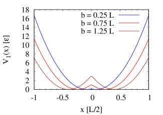
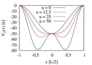
Figure 1: The shapes of the potentials $V_{1}(x)$ from Eq. (12) (top panel) and $V_{2}(x)$ from Eq. (13) (bottom panel) for different values of parameters.

III Comparison of exact and LDA coefficients

To perform a comparison between the LDA results and the exact solutions for the exchange coupling constants $\alpha_{i}$ we use two specific forms of a double well potential which have flexibility to explore the similarities and differences between the LDA and the exact calculation. The first potential has the form

$$V_{1}(x)=\frac{1}{2}k(|x|-b)^{2},$$ (12)

where $k$ and $b$ define the energy scale, and the height of the central barrier. Notice that this potential has a cusp (discontinuity of the first derivative) at $x=0$. This is perfectly well allowed in the formalism as this will not cause any troubling discontinuities in the single-particle wave functions or their first derivatives. The second potential is a symmetric trap of the form volosniev2014

$$V_{2}(x)=-V_{0}\sin^{2}\left[\frac{\pi}{2}\left(\frac{2x}{L}+1\right)\right]-u\sin^{2}\left[\pi\left(\frac{2x}{L}+1\right)\right],$$ (13)

where the values of $V_{0}$ and $u$ control the shape of the potential. Figure 1 shows the shapes of the potentials we use in the article for different values of the control parameters.

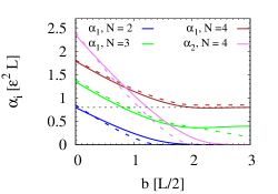
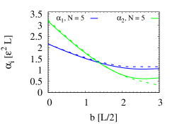
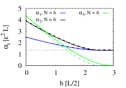
Figure 2: Geometric exchange coupling coefficients $\alpha_{i}$ for the double well potential in Eq. (12) with $k=1$ as function of the central barrier height $b$. The exact values based on the expression in Eq. (4) are shown as solid lines, while the corresponding approximate values based on the LDA formula in Eq. (6) are the dashed lines. The top panels shows $N=2,3$ and 4, the middle panel has $N=5$, and the bottom panel has $N=6$. Note that the parity symmetry of Eq. (12) implies that $\alpha_{N-i}=\alpha_{i}$. The dashed horizontal lines in the $N=4$ and $N=6$ cases correspond to the value $\alpha_{1}$ for $N=2$ and $N=3$, respectively. This is the excepted asymptotic values for large $b$ as discussed in the text.

We note that we consider values in the interval $x\in[-L/2;L/2]$ where $L$ is the length of a box which confines the whole system. This is required for our numerical procedure where we use $L=4\pi$ in our calculations. Energies are measured in units of $\epsilon=4\hbar^{2}/mL^{2}$, with a factor of 4 coming from the box extending to $\pm L/2$ For the potential in Eq. (12) we set $k=1$ (in units of $L$ and $\epsilon$) while for Eq. (13) we have used $V_{0}=50$ in units of $\epsilon$. In deep enough potentials the single-particle states do not feel the effect of this ’outside’ boundary. However, for shallow potentials some of the states might reside in the whole box and thus be influenced by the outer wall. We will see how it affects the exchange constants in the subsections below.

III.1 Results

We now consider the coefficients $\alpha_{i}$ using Eqs. (4) and  (6) for different values of the control parameters; the height of the central barrier $b$ for the potential in Eq. (12) and the parameter $u$ for the potential in Eq. (13). Figs. 2 and 3 show both the LDA and exact values of the coefficients $\alpha_{i}$ for different numbers of particles $N=2-6$. In this article we consider only spatially symmetric 1D potentials and so $\alpha_{N-i}=\alpha_{i}$.

In Fig. 2 we show the results for the potential in Eq. (12) comparing the exact results obtained from Eq. (4) to the LDA results obtained with the formula in Eq. (6) for particle numbers $N=2-6$. Note that we do not need to plot all the $\alpha_{i}$ coefficients as the parity invariance of the double well in Eq. (12) gives us the convenient symmetry relation $\alpha_{N-i}=\alpha_{i}$. The results demonstrate that the LDA does very well for small values of the central barrier height $b$ which should not be too surprising as the potential for small $b$ resembles very much that of a harmonic oscillator which was previously shown to be quite accurately described within LDA deuret2014 .

One notices that for the even particle numbers the middle coefficient, i.e. $\alpha_{1}$, $\alpha_{2}$, and $\alpha_{3}$ for $N=2$, $N=4$, and $N=6$, respectively, has similar behavior, and that this behavior is not captured well by the LDA for $b\gtrsim 0.75$. In fact, this middle coefficient, $\alpha_{N/2}$, calculated via Eq. (6) goes to zero much faster than the exact value. This $\alpha_{N/2}$ pertains to the exchange coupling in the middle of the trap, i.e. to the exchange taking place right at the central barrier in the potential. It is therefore determined by the probability for particle tunneling through this central barrier, and we clearly see the LDA fail to capture this effect for larger barriers, i.e. larger values of $b$, where LDA underestimates exchange. This is connected to the fact that LDA and in particular the Thomas-Fermi density in Eq. (7) is only well-defined in between the classical turning points, where $\mu-V(x)>0$. Hence for large barriers where $\mu-V(x)\leq 0$, the Thomas-Fermi density goes to zero and thus in turn the coefficient $\alpha_{N/2}$ goes to zero. For example, in the case of the potential in Eq. (12) $\alpha^{(lda)}_{N/2}\equiv 0$ for $b>\sqrt{N}$ (when $k=1$ as we have here). The termination values of $b=\sqrt{2}$, $b=2$, and $b=\sqrt{6}$ can be clearly seen on the horizontal axis for $\alpha_{1}$ ($N=2$) and $\alpha_{2}$ ($N=4$) in the top panel of Fig. 2, and for $\alpha_{3}$ ($N=6$) in the bottom panel of Fig. 2.

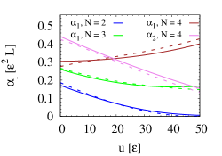
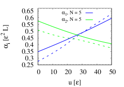
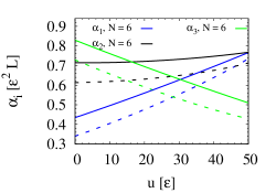
Figure 3: Geometric exchange coupling coefficients $\alpha_{i}$ for the smooth double well potential in Eq. (13) as function of the parameter $u$ that controls the central barrier. Here we have set $V_{0}=50$. The exact values based on the expression in Eq. (4) are shown as solid lines, while the corresponding approximate values based on the LDA formula in Eq. (6) are shown as dashed lines. The top panel shows $N=2,3$ and 4, the middle panel has $N=5$, and the bottom panel has $N=6$. Note that the parity symmetry of Eq. (13) implies that $\alpha_{N-i}=\alpha_{i}$.

When the height of the barrier is large (large $b$) each of the two wells can be approximated by the harmonic oscillator potential. We see that in this case the exact values of the coefficients becomes almost constant as function of the barrier height. For even number of particles we intuitively expect that half of the particles will be located in each well. In the case with $N=4$ this would imply that $\alpha_{1}$ should go to a constant for large $b$, reaching the value corresponding to the $b=0$ case with $N=2$ (two particles in a single harmonic well). This is clearly seen in the top panel of Fig. 2 where the horizontal dashed line marks the latter value. Likewise, for $N=6$, we expect a split into two three-body systems and thus that both $\alpha_{1}$ and $\alpha_{3}$ should be approaching the $\alpha_{1}$ value for $b=0$ and $N=3$. Again this is seen very nicely in the bottom panel of Fig. 2 the first two coefficients for $N=6$ approach the dashed horizontal line corresponding to $N=3$ and $b=0$ (notice that there are different vertical scales on the three panels in Fig. 2).

For the spatially symmetric potentials considered here with an odd number of particles, we cannot use the same logic of division of the particles into the two wells as the barrier grows large as for even particle numbers. The overlap across the barrier of the single-particle wave functions will not vanish for odd particle numbers. Hence, the coefficients $\alpha_{i}$ which depend solely on these single-particle wave functions will also not vanish. We clearly see in the top and the middle panel of Fig. 2 that for $b\gtrsim 2$ the LDA result does not do a good job in describing the exchange couplings. Again, this is caused by the fast decrease of the Thomas-Fermi density on which the LDA result relies as the barrier increases. This decrease of density clearly takes place much faster than seen in the exact results. We thus see that odd-even effects can be considerable in the comparison of the LDA and the exact method.

In order to further explore the case with odd particle numbers we have tried to apply a small tilt to the potential in order to explicitly break the parity invariance. This could for instance be done by an additional term that is linear in $x$ in the potential (12). When this is done for an odd number of particles the values of the exchange couplings approach the values of the couplings of a smaller system. For instance, for the system consisting of $N=5$ particles, two of the particles will be located in one of the wells, with the interacting coefficient approaching the value of $\alpha_{1}$ for two particles in a harmonic trap, and the other three will occupy the other well, with $\alpha_{1}=\alpha_{2}$ approaching those of a three-particle system in a harmonic trap. At the same time we find the intuitive result, namely that the interaction between these two subsystems will approach zero as the barrier increases. We will not discuss the introduction of slight symmetry-breaking terms any further here. All in all, for the double well potential (12) the LDA approach provides a reliable approximation to the exact values of the coefficients $\alpha_{i}$ for small central barrier heights (small values of $b$) and then becomes poor for larger barrier heights. An exception is found for even particles numbers where the system splits into two equal size groups that can be described as particles in two separate harmonic wells. Here LDA does approach the exact results for the split system asymptotically.

To further explore the robustness and/or failures of applying the LDA to our problem system, we now change the potential into a different kind of double well shape which has the form given in Eq. (13). What one should notice here is that the potential in Eq. (13) is in a sense shallow, i.e. it does not increase to infinity around its edges. Therefore the box potential that we have as a hard-wall boundary around the system could be felt by the particles. This is in fact the case for larger particle numbers as we will now discuss.

$N$	$\alpha_{i}^{(EXACT)}[\epsilon^{2}L]$	$\alpha_{i}^{(LDA)}[\epsilon^{2}L]$
$2$	$0.02487$	$0.01328$ (47%)
$3$	$0.06963$	$0.04485$ (36%)
$4$	$0.14921$	$0.10630$ (29%)
$5$	$0.27355$	$0.20798$ (24%)
$6$	$0.45260$	$0.35911$ (21%)

Table 1: Comparison of the exact calculation, $\alpha_{i}^{(EXACT)}$ (first column), to that of the LDA, $\alpha_{i}^{(LDA)}$ (second column), for a potential consisting of a flat box with infinite walls. Notice that in this case the exchange coefficients are independent of $i$, i.e. $\alpha_{i}=\alpha$. The percentages in parenthesis in the second column give the deviations of the LDA from the exact results. Notice that the LDA always underestimates the exchange coupling coefficients.

First we consider the cases with $N=2$ and $N=3$ as shown in the top panel of Fig. 3. Here we see that the qualitative behavior of the $\alpha_{i}$ coefficients is similar to the potential of Eq. (12) (shown in the top panel of Fig. 2) with the two-particle case shown a steady decrease with the barrier parameter, $u$, while the three-particle case first decreases and then has a slight increase again at large values of $u$. This is analogous to the behavior in the top panel of Fig. 2. We also notice that the LDA does a very good job for the two- and three-particle systems for most values of $u$ in the top panel of Fig. 3. For the $N=3$ case this should be compared and contrasted to the case in the top panel of Fig. 2 where the same $N=3$ case for the potential in Eq. (12) demonstrates that the LDA deviates significantly from the exact result for larger barrier heights (large $b$ values in that case).

For more particles ($N\geq 4$) the LDA results start to deviate significantly from the exact results as we see in all three panels in Fig. 3. We see that already for four particles the coefficient $\alpha_{i}$ differs significantly in the LDA and exact calculations. This difference only increases for larger particle numbers. The reason for this discrepancy can be traced back to the form of the potential in Eq. (13) and its shallow nature as compared to that in Eq. (12). For the parameters we have chosen, the potential does not become deep enough for five or six single-particle eigenstates to be confined completely inside of the potential profile. This can be rephrased by stating that not all the five or six lowest single-particle energy eigenvalues are in fact negative. The most energetic single-particle wave functions that we require to build the totally antisymmetric function, $\Psi_{0}$, are thus feeling the outside of the potential. In particular, they are influenced by the box potential that surrounds our system. While one may alleviate this problem by going to deeper potentials (increasing $V_{0}$ in Eq. (13)) we choose $V_{0}=50$ in order for us to study quantum state transfer in the last part of our paper and make contact with recent results that utilize the same parameters volosniev2014 .

To gain further insights into the influence of the box and the behavior of LDA in this respect we may consider just the box potential on its own. In Tab. 1 we present the results of applying both the exact formula (first column) and the LDA version (second column )to the box potential. We clearly see a large discrepancy for the particle numbers we have studied. The deviation of the LDA from the exact result is given in percentages in the parenthesis in the second column of Tab. 1. By doing a crude fit to the percentages we find that the deviations scale approximately with the particle number as a power law $N^{-0.73}$. We thus find a quite slow convergence and for smaller system sizes the deviations can be significant. We can see that as the single-particle wave functions are distributed over the whole confining infinite square well potential the local density approach becomes rather inadequate. The large discrepancies in the values of the LDA and the exact results for the $\alpha_{i}$ coefficients of the shallow potential in Eq. (13) for particle numbers $N\geq 5$ can now be better understood. They are in large part the result of the fact that the outer box boundaries do become important for these particles numbers and that the LDA does a poor job of describing particles in a box with a flat bottom. We do see that the LDA approximation gives qualitatively similar results to the exact calculation even for $N>4$, but quantitatively the LDA may differ substantially. We have checked that as one increases the depth of the potential in Eq. (13) one does indeed see better agreement. However, the deviations we identified as common for both potential profiles within the LDA remain.

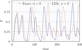
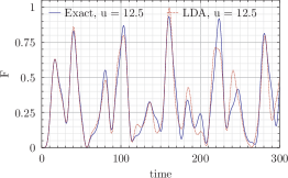
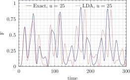
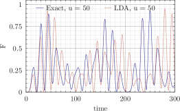
Figure 4: Quantum state transfer fidelity, $F$, for an $N=4$ two-component Fermi system with $J_{i}$ obtained from the potential in Eq. (13) for $u=0$ (first row), $u=12.5$ (second row), $u=25$ (third row), and $u=50$ (fourth row) where $u$ is in units of $\epsilon$. The other potential parameter is $V_{0}=50$ for all panels. The (blue) solid line corresponds to the $J_{i}$ coefficients obtained from the exact calculation and the (brown) dashed line corresponds to the LDA approach. Time is measured in units of $\hbar/\epsilon$.

IV Quantum transport properties

In order to understand some potential effects that could be implied by using the LDA instead of the exact solutions for the exchange couplings, we now consider a dynamical protocol that has recently been discussed in the context of strongly interacting systems in 1D. As mentioned earlier, one may indeed map these systems into effective spin models volosniev2013 ; deuret2014 . This can be done for both Fermi systems volosniev2013 ; deuret2014 ; levinsen2014 and Bose systems volosniev2014 ; pietro2015 . To keep the discussion concise, we will mainly consider the example of the two-component Fermi system here. In that case, the spin mapping is into the famous Heisenberg spin-$\tfrac{1}{2}$ model whose Hamiltonian (up to a constant energy shift) is given by

$$H_{s}=\sum_{j=1}^{N-1}J_{j}\bm{S}^{j}\cdot\bm{S}^{j+1},$$ (14)

where $\bm{S}^{j}=\frac{1}{2}\bm{\sigma}^{j}$ is a spin operator where $\bm{\sigma}^{j}=(\sigma_{x}^{j},\sigma_{y}^{j},\sigma_{z}^{j})$ is the vector of the Pauli matrices. Here the nearest-neighbor interaction coefficients are related very simply to the local exchange coefficients and the coupling constant as $J_{i}\equiv-\frac{\alpha_{i}}{g}$. This is another justification for using the term ’local exchange coupling’ for the $\alpha_{i}$ above, i.e. that under the spin mapping they appear as nearest-neighbor couplings in what is equivalent to a spin chain Hamiltonian. For Bose systems, one may have more involved spin models as the coefficients for $x$-, $y$-, and $z$- direction spin operators are not necessarily the same (see Ref. volosniev2014 for further details). Below, we will make one detour from the uniform Heisenberg spin model in Eq. (14) in order to consider the so-called XX model which is a special case of the Hamiltonian in Eq. (14) where all the terms with $z$-component operators are eliminated.

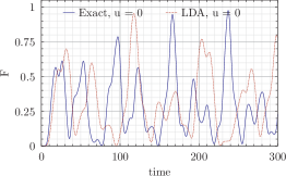
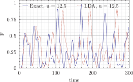
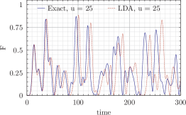
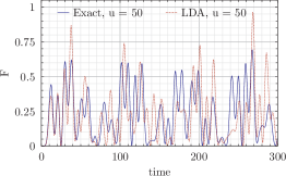
Figure 5: Same as Fig. 4 but for $N=5$.

Spin-$\tfrac{1}{2}$ chains have been proposed as media for quantum state transfer about a decade ago bose2003 ; bose2008 ; christandl2005 . The quantum state transfer in these chains essentially corresponds to flipping a single spin at one end of the chain and then dynamically evolving the state such that one may project onto the state at which the single spin flip has reached the other end for all subsequent times. The probability of finding the flipped spin at the other end is known as the fidelity of the quantum state transfer and if it reaches unity at some subsequent time we say that the system supports perfect quantum state transfer bose2008 . In the original proposal bose2003 a spin chain with constant $J_{i}=J$ was considered and it was shown that the fidelity could not reach unity in this case. Later studies demonstrated that if the coefficients are chosen as $J_{i}=J_{0}\sqrt{N(N-i)}$ with $J_{0}$ some overall constant, then perfect state transfer is possible (although only within the so-called XX model). One would then have an ideal communications channel for quantum information. However, it turns out to be exceedingly difficult to produce a system that fulfills these requirements on $J_{i}$. In Ref. volosniev2014 Volosniev et al. proposed strongly interacting 1D atomic systems as a possible realization of perfect state transfer and found that the potential in Eq. (13) can give rise to perfect state transfer in the XX model for $u=12.5$. We will return to this below. First we need to define the spin state space and the fidelity that we consider. For a spin chain with one impurity (a single spin that is flipped) and $N-1$ majorities (in other words $N_{\uparrow}=1$ and $N_{\downarrow}=N-1$) it is natural to use the basis of spin functions $\left\{\left|\uparrow\downarrow\downarrow\ldots\downarrow\right\rangle,\left|\downarrow\uparrow\downarrow\ldots\downarrow\right\rangle,\left|\downarrow\ldots\downarrow\uparrow\downarrow\right\rangle,\left|\downarrow\ldots\downarrow\downarrow\uparrow\right\rangle\right\}$. In this basis we define the fidelity of the quantum state transfer which is a function of time and is given by

$$F(t)=\left|\left\langle\downarrow\ldots\downarrow\downarrow\uparrow\right|e^{-iH_{s}t/\hbar}\left|\uparrow\downarrow\downarrow\ldots\downarrow\right\rangle\right|^{2}.$$ (15)

The fidelity can be straightforwardly interpreted as the Hamiltonian acting on the initial state on the right (with the single flipped spin on the left edge of the systems) and then projection on the final state on the left (with the single flipped spin on the right edge). In practice, one expands the initial state on the set of eigenstates of the Hamiltonian, then constructs the state at all later times, and then projects onto the final state which also has some expansion in terms of the eigenstates of the Hamiltonian. Notice that the overall time scale of the transfer depends on $\alpha_{i}$ and on $g$. In the strict limit where $1/g=0$, there is no dynamics as the particles are completely impenetrable and all orderings are eigenstates (all of which are degenerate). However, in the more realistic case where $g$ is large but finite, our effective spin models work to linear order in $1/g$ and can thus be used to study dynamics in the strongly interacting regime. The timescale of transfer will then depend linearly on $g$. One may think of the state transfer process as a set of subsequent flips of pairs of spins along the chain. Each of these local exchanges depend on $\alpha_{i}$, i.e. if $\alpha_{i}$ is large this happens fast and vice versa. We thus see that large barriers will suppress the transfer as expected. However, the process can depend rather delicately on the actual values of the local exchanges as we will now demonstrate. For instance, in the exact results we may see slow suppression of the local exchange with barrier height as in Fig. 2 in regimes where LDA would give exactly zero (when the chemical potential is below the barrier). This is one source of error in the LDA that could carry into a dynamical protocol like state transfer in a severe way.

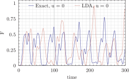
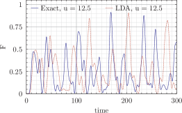
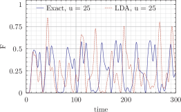
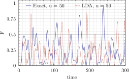
Figure 6: Same as Fig. 4 but for $N=6$.

Here we plot the fidelity of Eq. (15) as a function of time for different potentials of the form given in Eq. (13) for the cases with $N=4$ (Fig. 4), 5 (Fig. 5), and 6 (Fig. 6) particles, respectively. All the three cases we present show the characteristic oscillatory behavior of state transfer fidelities as function of time volosniev2014 . However, one does indeed notice that the oscillations become more prominent and more irregular as $N$ increases (system size or chain length in the spin chain language), and also as the control parameter for the central barrier $u$ is increased. Perfect state transfer is never achieved for these parameters in a Heisenberg model of the type in Eq. (14) without an external magnetic field. This is in accordance with previous results christandl2005 ; christandl2004 ; nikolopoulos2004 . The calculations demonstrate that even when there are only small differences in the exact and LDA results, the fidelity can show large variations particularly for longer time intervals. This is probably due to an accumulation of phase factors in the system over time that tends to drive the exact and LDA results apart. However, we do see some instances of very good agreement as for instance in the second row of Fig. 4 where $u=12.5$ and $V_{0}=50$ in Eq. (13). Even in this case, noticeable differences between exact and LDA results are seen, but the overall agreement is very good. For the larger particle numbers in Figs. 5 and 6 we may even notice a clear tendency for the LDA results to predict large fidelity spikes that are either at different times as compared to similar spikes using the exact result, or in some instances the LDA shows spikes where the exact results have none (see for instance the fourth row in Fig. 5 or the third row in Fig. 6). We thus conclude that in most cases, the LDA results can provide large deviations from the exact results in a dynamical process such as quantum state transfer.

In closing this section, we want to consider how well the LDA results do in the case where perfect state transfer is achieved. This can be achieved with parameters corresponding to the second row in Fig. 4 in a setup where we can discard the $\bm{S}_{z}^{j}\bm{S}_{z}^{j+1}$ interaction in the Hamiltonian in Eq. (14) and thus reduce the problem to the Heisenberg XX model. This can be realized by either using a tailored external magnetic field applied to the system or in specific models with strongly interacting two-component Bose systems volosniev2014 . In Fig. 7 we compare the fidelities computed using the exact and the LDA values of the exchange coupling coefficients. We see that the perfect transfer is indeed obtained for the values calculated via Eq. (4). However, the fidelity of the spin transfer decreases with time for the coefficients obtained via Eq. (6). The relative differences in the $\alpha_{i}$ exchange coefficients are no more than $2$ percent when comparing the exact to the LDA method. However, we still see that it affects the quantum transfer properties on longer time scales significantly.

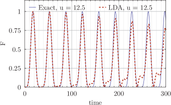
Figure 7: Quantum state transfer fidelity, $F$, for an $N=4$ two-component Fermi system with $J_{i}$ obtained from the potential in Eq. (13) for $u=12.5$ and $V_{0}=50$ (in units of $\epsilon$) for the case where the $z$-components in Eq. (14) can be discarded so that we are in the so-called Heisenberg XX spin model. In this case perfect state transfer can be achieved volosniev2014 . The (blue) solid line corresponds to the $J_{i}$ coefficients obtained from the exact calculation and the (brown) dashed line corresponds to the LDA approach. Time is measured in units of $\hbar/\epsilon$.

V Summary and discussion

We have considered strongly interacting two-component systems in one dimension held in place by an external confinement. Such systems have an effective Hamiltonian that can be completely specified by computing a set of local exchange coefficients which may be interpreted as nearest-neighbor spin exchange interactions when the system is mapped onto a spin model Hamiltonian of the Heisenberg type. Computing these exchange coefficients as accurately as possible is an important yet also computationally difficult task. In the present paper we have explored two different approaches. One is a ’brute force’ calculation of a multi-dimensional integral which gives the exact result (but is prohibitive for larger particle numbers) and the other is an approach inspired by the local density approximation (LDA) that could in principle be used to reduce the computational complexity. While previous studies have shown that the local density approach can be accurate at the level of a few percent for the case of a harmonic oscillator potential, we explore more complicated geometries consisting of two instances of a double-well potential.

Our findings demonstrate that while the LDA does rather well with potentials that resemble a harmonic oscillator, the exchange couplings do not have the right qualitative and quantitative behavior in the LDA when there are significant barriers as is typical of a double-well potential. In particular, the LDA cannot capture the right quantum tunneling processes across such barriers and may thus leave out important effects. We have shown that for small systems this can lead to an underestimation of exchange by the LDA for potentials which have a more interesting structure than the simple single-well harmonic oscillator. We expect this observation to have influence on experiments with small system sizes in 1D optical lattices. There one typically also has an external overall smooth potential (approximately harmonic in shape). Thus, the potential seen by the particles is the superposition of harmonic trap and optical lattice, i.e. a ’smiling’ lattice potential. This is a very structured potential and in the strongly interacting regime one could be in dire straits with a simple LDA approach as compared to the exact exchange couplings. In order to test out the LDA in a concrete physical process, we considered quantum state transfer of single spin flips in systems with four, five, and six particles. Here we found that while the LDA performs reasonably for some double-well realizations there is amplification of the deviations of the LDA compared to the exact results in the transfer fidelity that can be significant and lead to large errors in both maximum fidelity values and the specific times at which these are attained.

The current study has concentrated on small particle numbers where very accurate results can be obtained for the local exchange coefficients using multi-dimensional integration so that a comparison between exact and LDA results is possible for arbitrary potentials. Incidentally, as we discussed in the introduction, the system sizes used here are also of great current experimental interest in cold atoms. One would, however, like to study how these results scale to larger particle numbers. This most likely requires alternative approaches not only to the exact formula but also to the LDA formula. In the current implementation it depends on the density of the system which is not easy to compute for arbitrary potentials. One may thus pursue an agenda of finding an alternative LDA method that obtains the density by some other and computationally much simpler approach, and simultaneously explore how to get a computational reduction of the exact formula.

The authors gratefully acknowledge discussions with and feedback from A. G. Volosniev, M. Valiente, D. Petrosyan, N. J. S. Loft, A. E. Thomsen, and L. B. Kristensen. This work was supported by the Danish Council for Independent Research DFF Natural Sciences and the DFF Sapere Aude program.

References

- (1) I. Bloch, J. Dalibard, and W. Zwerger, Rev. Mod. Phys. 80, 885 (2008).
- (2) M. Lewenstein et al., Adv. Phys. 56, 243 (2007).
- (3) T. Esslinger, Ann. Rev. Cond. Mat. Phys. 1, 129 (2010).
- (4) Y. Nishida and D. T. Son, Phys. Rev. D 76, 086004 (2007); D. T. Son, Phys. Rev. D 78, 046003 (2008).
- (5) K. Balasubramanian and J. McGreevy, Phys. Rev. Lett. 101, 061601 (2008); J. Maldacena, D. Martelli,and Y, Tachikawa, J. High Energy Phys. 10 (2008) 072; A. Adams, K. Balasubramanian, and J. McGreevy, J. High Energy Phys. 11 (2008) 059.
- (6) N. T. Zinner and A. S. Jensen, J. Phys. G:Nucl. Part. Phys. 40, 053101 (2013).
- (7) M. A. Baranov, M. Dalmonte, G. Pupillo, and P. Zoller, Chem. Rev. 112, 5012 (2012).
- (8) H. Moritz, T. Stöferle, M. Köhl, and T. Esslinger, Phys. Rev. Lett. 91, 250402 (2003).
- (9) T. Stöferle, H. Moritz, C. Schori, M. Köhl, and T. Esslinger, Phys. Rev. Lett. 92, 130403 (2004).
- (10) T. Kinoshita, T. Wenger, and D. S. Weiss, Science 305, 1125 (2004).
- (11) B. Paredes et al., Nature 429, 277 (2004).
- (12) T. Kinoshita, T. Wenger, and D. S. Weiss, Nature 440, 900 (2005).
- (13) E. Haller et al., Science 325, 1224 (2009).
- (14) E. Haller et al., Nature 466, 597 (2010).
- (15) M. Olshanii, Phys. Rev. Lett. 81, 938 (1998).
- (16) L. W. Tonks, Phys. Rev. 50, 955 (1936).
- (17) M. D. Girardeau, J. Math. Phys. 1, 516 (1960).
- (18) G. Pagano et al., Nature Phys. 10, 198 (2014).
- (19) F. Serwane et al., Science 332, 336 (2011).
- (20) G. Zürn et al., Phys. Rev. Lett. 108, 075303 (2012).
- (21) G. Zürn et al., Phys. Rev. Lett. 111, 175302 (2013).
- (22) A. Wenz et al., Science 342, 457 (2013).
- (23) S. Murmann et al., Phys. Rev. Lett. 114, 080402 (2015).
- (24) S. Murmann et al., Phys. Rev. Lett. 115, 215301 (2015).
- (25) S. Zöllner, H.-D. Meyer, and P Schmelcher, Phys. Rev. A 74, 063611 (2006); Phys. Rev. A 75, 043608 (2007); Phys. Rev. Lett. 100, 040401 (2008).
- (26) F. Deuretzbacher, K. Bongs, K. Sengstock, and D. Pfannkuche, Phys. Rev. A 75, 013614 (2007).
- (27) E. Tempfli, S. Zöllner, and P. Schmelcher, New J. Phys. 11, 073015 (2009).
- (28) M. D. Girardeau, Phys. Rev. A 83, 011601(R) (2011).
- (29) I. Brouzos and P. Schmelcher, Phys. Rev. Lett. 108, 045301 (2012).
- (30) I. Brouzos and A. Förster, Phys. Rev. A 89, 053632 (2014).
- (31) B. Wilson, A. Förster, C. C. N. Kuhn, I. Roditi, and D. Rubeni, Phys. Lett. A 378, 1065 (2014).
- (32) N. T. Zinner et al., Europhys. Lett. 107, 60003 (2014).
- (33) M. A. Garcia-March et al., Phys. Rev. A 92, 033621 (2015).
- (34) A. S. Dehkharghani et al., Scientific Reports 5, 10675 (2015).
- (35) P. Massignan, J. Levinsen, and M. M. Parish, Phys. Rev. Lett. 115, 247202 (2015).
- (36) L. Guan, S. Chen, Y. Wang, and Z.-Q. Ma, Phys. Rev. Lett. 102, 160402 (2009).
- (37) C. N. Yang, Chin. Phys. Lett. 26, 120504 (2009).
- (38) X.-W. Guan and Z.-Q. Ma, Phys. Rev. A 85, 033632 (2012).
- (39) D. Rubeni, A. Förster, and I. Roditi, Phys. Rev. A 86, 043619 (2012).
- (40) I. Brouzos and P. Schmelcher, Phys. Rev. A 87, 023605 (2013).
- (41) P. O. Bugnion and G. J. Conduit, Phys. Rev. A 87, 060502(R) (2013).
- (42) S. E. Gharashi and D. Blume, Phys. Rev. Lett. 111, 045302 (2013).
- (43) T. Sowiński, T. Graß, O. Dutta, and M. Lewenstein, Phys. Rev. A 88, 033607 (2013).
- (44) S. E. Gharashi, X. Y. Yin, and D. Blume, Phys. Rev. A 89, 023603 (2014).
- (45) A. G. Volosniev et al., Few-Body Syst. 55, 839 (2014).
- (46) X. Cui and T.-L. Ho, Phys. Rev. A 89, 023611 (2014).
- (47) N. J. S. Loft et al., Eur. Phys. J. D 69, 65 (2015).
- (48) R. Lundmark, C. Forssén, and J. Rotureau, Phys. Rev. A 91, 041601(R) (2015).
- (49) S. E. Gharashi, X. Y. Yin, and D. Blume, Phys. Rev. A 91, 013620 (2015).
- (50) F. Nur Ünal, B. Hetényi, and M. Ö. Oktel, Phys. Rev. A 91, 053625 (2015).
- (51) A. G. Volosniev, H.-W. Hammer, and N. T. Zinner, arXiv:1507.00186 (2015).
- (52) M. D. Girardeau, Phys. Rev. A 82, 011607(R) (2010).
- (53) L. Guan and S. Chen, Phys. Rev. Lett. 105, 175301 (2010).
- (54) G. E. Astrakharchik and I. Brouzos, Phys. Rev. A 88, 021602(R) (2013).
- (55) A. G. Volosniev et al., Nature Commun. 5, 5300 (2014).
- (56) E. J. Lindgren et al., New J. Phys. 16, 063003 (2014).
- (57) F. Deuretzbacher et al., Phys. Rev. A 90, 013611 (2014).
- (58) A. G. Volosniev et al., Phys. Rev. A 91, 023620 (2015).
- (59) L. Yang, L. Guan, and H. Pu, Phys. Rev. A 91, 043634 (2015).
- (60) J. Levinsen, P. Massignan, G. M. Bruun, and M. M. Parish, Science Adv. 1, e1500197 (2015)
- (61) T. Sowiński, M. Gajda, and K. Rza̧żewski, Europhys. Lett. 109, 26005 (2015).
- (62) T. Grining et al., Phys. Rev. A 92, 061601 (2015).
- (63) M. D. Girardeau and M. Olshanii, Phys. Rev. A 70, 023608 (2004).
- (64) M. D. Girardeau and A. Minguzzi, Phys. Rev. Lett. 99, 230402 (2007).
- (65) S. Zöllner, H.-D. Meyer, and P Schmelcher, Phys. Rev. A 78, 013629 (2008);
- (66) X.-W. Guan, M. T. Batchelor, and J.-Y. Lee, Phys. Rev. A 78, 023621 (2008).
- (67) F. Deuretzbacher et al., Phys. Rev. Lett. 100, 160405 (2008).
- (68) B. Fang, P. Vignolo, M. Gattobigio, C. Miniatura, and A. Minguzzi, Phys. Rev. A 84, 023626 (2011).
- (69) N. L. Harshman, Phys. Rev. A 86, 052122 (2012).
- (70) M. A. Garcia-March and Th. Busch, Phys. Rev. A 87, 063633 (2013).
- (71) M. A. Garcia-March et al., Phys. Rev. A 88, 063604 (2013).
- (72) N. L. Harshman, Phys. Rev. A 89, 033633 (2014).
- (73) S. Campbell, M. A. Garcia-March, T. Fogarty, and Th. Busch, Phys. Rev. A 90, 013617 (2014).
- (74) M. A. Garcia-March et al., New J. Phys. 16, 103004 (2014).
- (75) P. D’Amico and M. Rontani, J. Phys. B 47, 065303 (2014); Phys. Rev. A 91, 043610 (2015).
- (76) N. P. Mehta, Phys. Rev. A 89, 052706 (2014).
- (77) M. A. Garcia-March et al., Phys. Rev. A 90, 063605 (2014).
- (78) R. E. Barfknecht, I. Brouzos, A. Förster, Phys. Rev. A 91, 043640 (2015).
- (79) A. G. Volosniev, H.-W. Hammer, and N. T. Zinner, Phys. Rev. A 92, 023623 (2015).
- (80) A. S. Dehkharghani, A. G. Volosniev, and N. T. Zinner, Phys. Rev. A 92, 031601(R) (2015).
- (81) N. L. Harshman, Few-body Syst. 57, 11 (2016); Few-body Syst. 57, 45 (2016).
- (82) D. Pęcak, M. Gajda, and T. Sowiński, New J. Phys. 18, 013030 (2016).
- (83) T. Graß, Phys. Rev. A 92, 023634 (2015).
- (84) A. S. Dehkharghani, A. G. Volosniev, and N. T. Zinner, arXiv:1511.01702 (2015).
- (85) D. S. Petrov, G. V. Shlyapnikov, and J. T. M. Walraven, Phys. Rev. Lett. 85, 3745 (2001).
- (86) A. Recati, P. O. Fedichev, W. Zwerger, and P. Zoller, Phys. Rev. Lett. 90, 020401 (2003).
- (87) G. E. Astrakharchik, D. Blume, S. Giorgini, and L. P. Pitaevskii, Phys. Rev. Lett. 93, 050402 (2004).
- (88) I. V. Tokatly, Phys. Rev. Lett. 93, 090405 (2004).
- (89) G. E. Astrakharchik, Phys. Rev. A 72, 063620 (2005); G. E. Astrakharchik, J. Boronat, J. Casulleras, and S. Giorgini, Phys. Rev. Lett. 95, 190407 (2005).
- (90) G. Orso, Phys. Rev. Lett. 98, 070402 (2007).
- (91) X.-J. Liu, H. Hu, and P. D. Drummond, Phys. Rev. A 78, 023601 (2008).
- (92) M. Colomé-Tatché, Phys. Rev. A 78, 033612 (2008).
- (93) G. De Rosi and S. Stringari, Phys. Rev. A 92, 053617 (2015).
- (94) M. Chenaeu et al., Nature 481, 484 (2012).
- (95) T. Fukuhara et al., Nature Physics 9, 235 (2013); T. Fukuhara et al., Nature 502, 76 (2013).
- (96) S. Hild et al., Phys. Rev. Lett. 113, 147205 (2014).
- (97) T. Fukuhara et al., Phys. Rev. Lett. 115, 035302 (2015).
- (98) S. Trotzky et al., Science 319, 295 (2008).
- (99) M. Ogata and H. Shiba, Phys. Rev. B 41, 2326 (1990).
- (100) K. A. Matveev, Phys. Rev. B 70, 245319 (2004).
- (101) X.-W. Guan, M. T. Batchelor, and M. Takahashi, Phys. Rev. A 76, 043617 (2007).
- (102) K. A. Matveev and A. Furusaki, Phys. Rev. Lett. 101, 170403 (2008).
- (103) S. Bose, Phys. Rev. Lett. 91, 207901 (2003)
- (104) S. Bose, Contemporary Physics, Volume 48, Issue 1, 13-30 (2007)
- (105) M. Christandl, et al., Phys. Rev. A 71, 032312 (2005)
- (106) M. Christandl, et al., Phys. Rev. Lett. 92, 187902 (2004)
- (107) G. M. Nikolopoulos, et al., Europhys. Lett. 65(3), 297-303 (2004)