A Dynamical Model of Twitter Activity Profiles

Abstract

The advent of the era of Big Data has allowed many researchers to dig into various socio-technical systems, including social media platforms. In particular, these systems have provided them with certain verifiable means to look into certain aspects of human behavior. In this work, we are specifically interested in the behavior of individuals on social media platforms—how they handle the information they get, and how they share it. We look into Twitter to understand the dynamics behind the users’ posting activities—tweets and retweets—zooming in on topics that peaked in popularity. Three mechanisms are considered: endogenous stimuli, exogenous stimuli, and a mechanism that dictates the decay of interest of the population in a topic. We propose a model involving two parameters $\eta^{\star}$ and $\lambda$ describing the tweeting behaviour of users, which allow us to reconstruct the findings of Lehmann et al. (2012) on the temporal profiles of popular Twitter hashtags. With this model, we are able to accurately reproduce the temporal profile of user engagements on Twitter. Furthermore, we introduce an alternative in classifying the collective activities on the socio-technical system based on the model.

ACM Categories and Subject Descriptors: J.2 [Computer Applications]: Physical Sciences and Engineering; J.4 [Computer Applications]: Social and Behavioral Sciences; I.6 [Computing Methodologies]: Simulation and Modeling

I Introduction

The study of information diffusion from gossip spreading Lind_2007a ; Lind_2007 , to the propagation of viral memes Ratkiewicz_2011 ; Shifman_2009 ; Hodas.Lerman:2014 , fads, and trends Tassier_2004 ; Altshuler_2012 ; Sano.etal:2013 , and even word-of-mouth marketing Goldenberg_2001 ; Legara_2008 has become increasingly interesting especially in this era of “Big Data.” Current technologies and methods have allowed researchers to look more closely into the social network fabric—the medium at which the proliferation of various entities takes place. Questions relating to how fast information travels or what kind of information captures the most audience have piqued the interest of many researchers Asur2011 ; Weng_2013 ; Louni_2014 ; Ikeda_2010 ; Chung_2014 . Various approaches have been implemented to shed light into these. Researchers have looked into the role of a network’s degree of connectivity, modularity, and various centrality measures, among other things Weng_2013 ; Louni_2014 ; Ikeda_2010 ; Chung_2014 . Efforts have also been put in understanding the degree of social “influence” of entities on each other Myers:2012 ; Granovetter_1978 ; Cosley:2010 . Many have also investigated the nature of topics that are being diffused in a social system.

In this work, we propose a model that aims to capture the various aspects of these approaches—we do not only look at the network structure in isolation, but also augment it with particulars on the nature of the information being spread, and the individuals’ tendencies to spread such information or “inject” new ones. Particularly, we investigate the observations described in Lehmann.etal:2012 on the dynamical classes of collective attention in Twitter where they defined four groups depending on the temporal features of their popularity dynamics. We initially introduce two free parameters intrinsic to the users’ behaviours, $\lambda$ and $\eta^{\star}$, where $\lambda$ quantifies the rate of decay at which a user would spread a given information and $\eta^{\star}$ is the threshold an agent has that determines whether or not he/she propagates information from the users he/she follows. The rules defined are then implemented in an empirical Twitter network obtained from the Stanford Large Network Dataset Collection McAuley_2012 .

This paper is structured as follows: we first describe the data and model in Sec. II, then present the results and discussions in Sec. III, and finally summarise and establish our conclusions in Sec. IV.

II Data and the model

II.1 Data

The dataset utilised here is a set of $115$ hashtags used by Lehmann et al. in Lehmann.etal:2012 . It contains the time series of number of tweets and distinct users for each of the hashtags. Each time series centers around a day on which the number of relevant tweets attain their maximum “popularity,” and spans from seven days before to seven days after the day of the peak. The full data collected in Lehmann.etal:2012 contain $130$ million Twitter messages appearing in the period of approximately $6$ months from November 20, 2008 to May 27, 2009. We point the readers to reference Lehmann.etal:2012 for further details on the dataset utilised here for model fitting and verification.

II.2 The model

II.2.1 Definitions and rules

The model is defined on a general network $\mathcal{N}$ with $N$ nodes, each node representing a user. Each user $i$ has $F_{i}$ “followers” and $L_{i}$ “leaders” whom he/she follows. This leader-follower relationship results to a directed network. It is also worth noting that although the Twitter network structure is dynamically changing in the real-world, here we only consider a static structure given the relatively short time frame we are considering, which is two weeks. Note that when a user $i$ follows another user $j$, the follower sees all the tweets that $j$ posts; if, on the other hand, user $i$ visits the profile page of $j$, $i$ will not only see the tweets, but also the retweets and replies that user $j$ posts.

Three mechanisms are incorporated in our model. Two of which, exogenous and endogenous, define the manner at which information is propagated in the system Lehmann.etal:2012 ; Sornette:2008 . The endogenous process involves a re-posting of someone else’s tweet (“retweet”), thereby propagating/diffusing the same tweet across the social network. On the other hand, when new information is “injected” in the social network system, an exogenous process is said to have taken place. In addition to these two mechanisms, a third one is regarded as well that accounts for the decay of the level of the activities involving a specific topic on Twitter. To encapsulate, our model incorporates these three processes: (1) injection of new information into the network, (2) spreading of information in the network, and (3) decay of information after a peak.

The key features of the model proposed are quantified in two parameters $\eta^{\star}$ and $\lambda$—characterising the spreading of information and the decay of activities in the network, respectively. The parameter $\eta^{\star}$ quantifies the threshold of influence of leaders on their followers, determining whether or not a follower would take action such as retweeting and/or replying to a tweet, consequently exposing his/her own followers to the information. In other words, $\eta^{\star}$ encapsulate the level of contagion of a piece of information in the network. On the other hand, the parameter $\lambda$ quantifies the rate of decay of interest of a user in the information after a certain point in time. It could be seen that, in our model, the build-up in activities before a topic’s peak in popularity is solely reflected by the parameter $\eta^{\star}$, while the decay in activities after the peak is the interplay between the two parameters $\eta^{\star}$ and $\lambda$.

To make the model results comparable with the data we have at hand, we use the scale of one day as one time unit. The rules and flowchart of implementation of the model are described in Fig. 1. The model is updated sequentially, i.e. the state of a user $i$ at time $t$ only depends on the state of the network before time $t$ but not at time $t$.

Figure 1: Rules of the model proposed in this work. $t_{0}$ is the day of the peak and $\eta$ is the amount of activities by the user’s leaders accumulated after his last tweet.

II.2.2 Assumptions

The model constructed makes the following assumptions on the tendency of a user to tweet and retweet. A user posts an original tweet if he/she is exposed to some new information outside of his/her Twitter network, i.e. from external sources (or has some original ideas to share). A user who follows a lot of other users tends to rely solely on his/her social network for information and, hence, retweets more often than “injects” new information from external sources. On the contrary, a user who has a huge following tends to be more active in posting original ideas or new tweets rather than just reposting others’. These assumptions on tendencies are illustrated in Fig. 2.

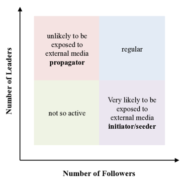
(a) Tweeting behaviour of different types of Twitter users based on their number of leaders and followers. Each type corresponds to the likelihood of being exposed to external media.

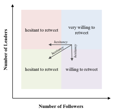
(b) Retweeting hesitancy of different types of Twitter users based on their number of leaders and followers. The arrows indicate the directions of increasing hesitancy, i.e. when the number of leaders or followers decreases.

Figure 2: Behaviour patterns of different types of users according to their number followers and leaders.

Let us consider a user $i$ ($i=1,2,\dots,N$) who follows $L_{i}$ leaders $l(i,j)$ ($j=1,2\dots,L_{i}$) and who has $F_{i}$ followers. The probability that user $i$ is exposed to external sources is

$$\boxed{\rho_{i}(t)=A_{i}\chi(t-t_{0})\text{,}}$$ (1)

in which $A_{i}$ represents the activeness of $i$ in following news and propagating to other people, and $\chi(t-t_{0})$ the coverage by the media. In general, the temporal profile of external media coverage satisfies the limiting conditions

$$\left\{\begin{aligned} 1\geq\chi(x)&\geq 0~{}\forall x\\ \chi(0)&=1\\ \lim_{\left|x\right|\rightarrow\infty}{\chi(x)}&=0\end{aligned}\right.\text{.}$$ (2)

We, however, assume that within a narrow window of time around the event, the media coverage is consistent and stays approximately constant so that $\chi(x\sim 0)\approx 1$. By the assumption described above, the activeness $A_{i}$ takes the form

$$A_{i}=\frac{F_{i}}{F_{max}}\times\left(1-\frac{L_{i}}{L_{max}+F_{i}}\right)$$ (3)

to reflect the assumption that a user having more followers tends to be active in following news and can introduce interesting stuff, but that is offset by having many leaders—as in such case, the user tends to rely on the leaders for information rather than tweeting so himself/herself as illustrated in Fig. 2(a) (see, for example, Kwak.etal:2010 ).

Upon external exposure, the probability of a user $i$ to tweet $T_{i}$ depends on: (1) the interest of user $\sigma_{i}$ in the nature of the information or the particular topic under consideration, (2) the level of interest $\tau_{i}(t-t_{0})$ as a function of time, and (3) his hesitancy to tweet $H_{i}$.

$$\boxed{T_{i}=\sigma_{i}\tau_{i}(t-t_{0})-H_{i}\text{.}}$$ (4)

The level of interest $\tau_{i}(t-t_{0})$ is high during and before the event, and decays with rate $\lambda$ after the event

$$\tau(x)=\left\{\begin{aligned} 1&\text{ if }x\leq 0\\ \exp{(-\lambda x)}&\text{ if }x>0\end{aligned}\right.\text{.}$$ (5)

The hesitancy to tweet (also retweet) depends on the number of leaders and followers a user has as illustrated in Fig. 2(b). The less leaders or followers a user has, the more hesitant he is to retweet because of the lack of engagement and/or motivation to do so. Hence,

$$H_{i}=\frac{1}{L_{i}+F_{i}+1}\text{.}$$ (6)

Here, we also assume that $\sigma=1$ indicating that we only focus on the topics that are of interest to the users.

Next, we define the average influence of all leaders of a user $i$ as

$$I_{i}=\frac{1}{L_{i}}\sum_{j=1}^{L_{i}}{F_{l(i,j)}}\text{,}$$ (7)

in which $F_{l(i,j)}$ is the number of followers that the leader $l(i,j)$ has.

In addition, we quantify the amount of exposure user $i$ has to the influence of his/her leaders in the following equation:

$$Y_{i}(t)=\sum_{\begin{subarray}{c}\text{all leaders}\\ l(i,j)\text{ having}\\ \text{tweeted}\\ \text{recently}\\ \text{before }t\end{subarray}}{F_{l(i,j)}}\text{.}$$ (8)

And the necessary condition for retweeting is

$$\boxed{Y_{i}\geq\eta^{\star}I_{i}\text{.}}$$ (9)

Upon this condition is met, the user $i$ retweets with probability

$$\boxed{R_{i}(t-t_{0})=\sigma_{i}\tau_{i}(t-t_{0})-H_{i}\text{,}}$$ (10)

which takes the same form as Eq. (4) in which $H_{i}$ represents the hesitancy as described in Eq. (6).

The number of leaders who tweeted recently, i.e. after the user’s last tweet and before current time $t$, is denoted as $\eta_{i}(t)$. The total number of possible retweets by user $i$ at time $t$ is given by

$$\boxed{\nu_{i}(t)=\sqrt{\frac{\eta_{i}(t)}{\eta^{\star}}\times\frac{Y_{i}}{\eta^{\star}I_{i}}}\text{,}}$$ (11)

in which we only take the integer part and take $0$ as $1$ because the number of retweets is at least $1$ if the user retweets.

If the user retweets, it does not necessarily mean that he would retweet all $n$ tweets. The probability to retweet $R$ means that he tweets at least one tweet. Therefore, it could be calculated that each of his $n$ possible retweets carries probability $r=1-\sqrt[n]{1-R}$.

By identifying the two key parameters $\lambda$ and $\eta^{\star}$, we can expect to observe four different types of users’ behaviour in response to an event, as illustrated in Fig. 3. The four types correspond to four quadrants in the $(\lambda,\eta^{\star})$ parameter space, namely lowly contagious-slow decaying, lowly contagious-fast decaying, highly contagious-slow decaying and highly contagious-fast decaying.

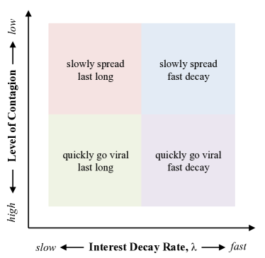
Figure 3: Distribution of different types of event in the $(\lambda,\eta^{\star})$ parameter space.

III Results and discussions

The empirical network we use for simulation was obtained from Stanford Large Network Dataset Collection McAuley_2012 . The entire network is a combination of $1,000$ ego networks with $81,306$ nodes and $1,768,149$ links, a diameter of $7$, and a clustering coefficient of $0.5653$. We run the simulation starting from $\delta t$ days before a topic peaks in popularity $t_{0}$ (we also refer to this one as “event”) until $7$ days after $t_{0}$. $\delta t$ can vary from $0$ to $7$, mimicking the fact that the amount of activities related to an event becomes significant up to $\delta t$ days before the event. $\delta t=0$ corresponds to sudden events while a large value of $\delta t$ indicates an anticipated one. It is noteworthy that by varying $\delta t$, we effectively include a third parameter in our model, which characterises the injection of information into the network.

We then scan the $(\lambda,\eta^{\star})$ parameter space in the steps of $\Delta\lambda=0.1$ ($\lambda\in[0;4]$) and $\Delta\eta^{\star}=1$ ($\eta^{\star}\in[1;60]$) to produce different time series for the number of tweets as well as the number of (distinct) users everyday and identify the ones that reproduce the empirical observations by using the distance metric introduced below. Since this is a Monte-Carlo simulation that involve generation of random numbers, we perform $50$ runs with distinct seeds for the random number generator for each set-up, i.e. the triplet $(\delta t,\eta^{\star},\lambda)$, and take the average results.

III.1 Validation of the model

We compare the data generated by our model to the empirical data by calculating the matching score of the two profiles which are quantified by the fraction of users or tweets on a single day. In details, let $\bm{P}=(P_{1},P_{2},\dots,P_{N})$ be the profile of the tweets produced by our model, i.e. $P_{i}$ is the fraction of tweets on day $t_{i}$ within the entire period from $t_{1}$ to $t_{N}$. By definition, we have

$$\sum_{i=1}^{i=N}{P_{i}}=1\text{.}$$ (12)

Similarly, $\bm{Q}=(Q_{1},Q_{2},\dots,Q_{N})$ is the corresponding profile of the tweets in the data collected by Lehmann.etal:2012 .

We compare $\bm{P}$ and $\bm{Q}$ by introducing the metric

$$\delta(\bm{P},\bm{Q})=\frac{1}{N}\sqrt{\sum_{i=1}^{i=N}{\left(\frac{P_{i}-Q_{i}}{\max{(P_{i},Q_{i})}}\right)^{2}}}\text{,}$$ (13)

which quantifies the (normalised) “distance” between the two profiles. It is obvious that when the two profiles are identical $\bm{P}\equiv\bm{Q}$, i.e. $P_{i}=Q_{i}~{}\forall i=1,2,\dots,N$, the distance is $\delta(\bm{P},\bm{Q})=0$. This is a normalised measure so that the maximum possible value of $\delta$ is $1$.

In Eq. (13), when $P_{i}=Q_{i}=0$, the term $\displaystyle\left(\frac{P_{i}-Q_{i}}{\max{(P_{i},Q_{i})}}\right)^{2}$ does not have any contribution to $\delta$. Finally, we set a tolerance threshold $\theta=0.04$ such that all the terms with $P_{i}+Q_{i}\leq\theta$ do not have any contribution to $\delta$.

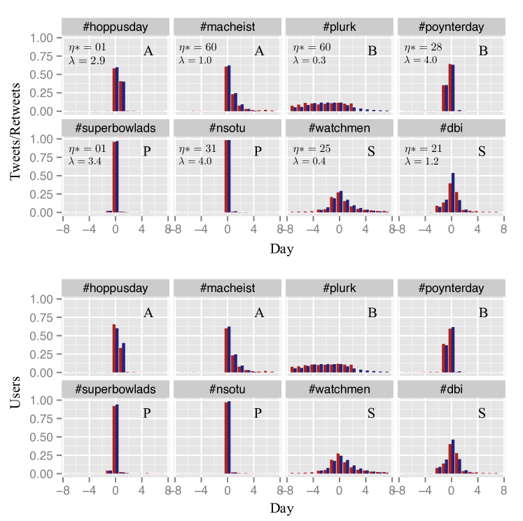
Figure 4: Time series of activities (top) and users (bottom). Results from the model (blue) shown together with the data (red) presented in Lehmann.etal:2012 for classes A, B, P, and S, respectively.

Using the metric introduced above and after visually verifying the plots (Fig. 4), we consider measures with $\delta(\bm{P},\bm{Q})\leq 0.08$ good and discard the rest. Of the $115$ hashtags, about $80\%$ ($88/115$) result to good fits—both for the number of users and number of retweets. The remaining $20\%$ fall into the groups of activities distributed before and symmetric around the peak day Lehmann.etal:2012 , which have significant amounts of activities distributed prior to the events. This demonstrates that the proposed model, in spite of it being capable of capturing the main features in the collective attention build-up and decay of users before and after the event day, requires additional framework that would quantify the “sense of time” of the users—whether or not an event is approaching Alfi.etal:2007 . This aspect will be investigated and reported elsewhere.

It is worth noting that while it is not straightforward to know how many times a user would tweet or retweet in a day, we have shown that our assumptions in Sec. II.2.2 for the users’ activities work well in estimating both the number of users and retweets in most cases. Moreover, the fact that we could reproduce the temporal profiles of activities (see Fig. 4) using our model with only two user-intrinsic parameters and an effective third parameter for external factors, justifies and validates our assumptions and hypotheses in identifying the key mechanisms of information spreading in social networks.

III.2 Classification of hashtag types

With the estimated parameter values, we generate the plot for the distribution of the hashtags on the two-dimensional parameter space of $\eta^{\star}$ and $\lambda$, as shown in Fig. 5. From the plot, we can observe the clustering pattern corresponding to different types of event shown in Fig. 3, with only a few outliers. It is quite evident that there is a clustering of large points at the bottom left corner of the plot, which correspond to the events that quickly go viral and last long. Those events appear many days before the peak and generate significant amount of activities afterward. The other three clusters contain small points signifying the events start not so long before their peak of activities.

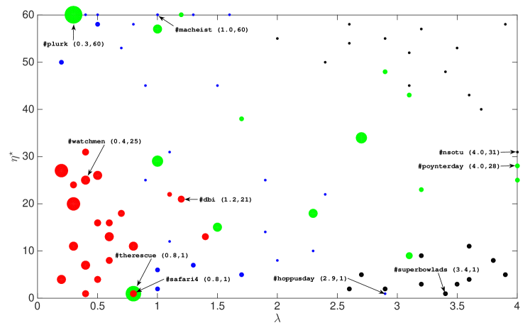
Figure 5: Fitted parameters $\eta^{\star}$ and $\lambda$ showing clustering patterns. The circles of larger size correspond to large value of $\delta t$. The colours (online) of the data points are determined by the classed identified in Lehmann.etal:2012 , red for S, black for P, blue for A and green for B.

As illustrated by the colors of the data points in Fig. 5, we can also observe that the distribution of the points correspond very well to the classification of dynamical classes reported in Lehmann.etal:2012 , i.e. the points for each of the four classes can be segregated into distinct clusters (with exception of a few points in class of activities concentrating before the peak, see below). The four classes are called A, B, P and S, respectively, in this work for convenience of the discussion. Class A describes events where the associated activities are concentrated after a topic peaks in popularity. Class B, on the other hand, refers to the events where the activities occur before the peaks. Class P consists of events where the activities are concentrated on a single day. Finally, Class S contains events that have significant activites before, on and after the peak day. Our results show that the clusters described above also reveal the existence of subclasses within each of the classes. In Fig. 5, we can generally identify $7$ clusters of data points (or hashtags) which show very good correspondence to the classification in Lehmann.etal:2012 .

From the fittings, we can observe two subgroups in the class with activities concentrating after the peak, i.e. class A (after). One group shows long range behaviours in which the activities span over a long period of time reflected by slow decay of interest (small $\lambda$) but high spreading threshold (large $\eta^{\star}$). The other group shows short range behaviours in which the activities span over a very short period of time reflected by low spreading threshold (small $\eta^{\star}$) but very fast decay of interest (large $\lambda$).

For the class with activities concentrating before the peak, i.e. class B (before), we also observe two subgroups. One group shows long range behaviours in which the activities span over a long period of time reflected by long appearance before the peak but high spreading threshold (large $\eta^{\star}$). The other group shows short range behaviours in which the activities span over a very short period of time reflected by very short appearance before the peak but very low spreading threshold (small $\eta^{\star}$).

For the class with activities concentrating at the peak, i.e. class P (peak), the values of the parameters suggest two subgroups, both of which have very fast decay of interest (large $\lambda$). One group shows contagious behaviours in which the events appear very shortly before the peak but generate a lot of activities due to low spreading threshold (small $\eta^{\star}$). The other group shows inert behaviours due to very high spreading threshold (large $\eta^{\star}$).

The class with activities distributed symmetrically around the peak, i.e. class S (symmetric), generally has low spreading threshold (small $\eta^{\star}$) and slow decay of interest (small $\lambda$).

In Fig. 4, we show the different profiles for each of the classes described above.

III.3 Content analysis

After revealing the existence of the classes and subclasses of the hashtags, we turn to looking at content of each hashtag and learn how it is related to the apparent classification. In Appendix A, we have a table showing the hashtags together with their corresponding type and class (and subclass, according to our results above). The table is organised in such a way that the top rows contain the “simple” hashtag types, in the sense that the hashtags of those types generally belong to one class identified by our model. The rows further down at the bottom of the table contain more complicated hashtag types whose tweets fall into different classes.

From the table, it could be seen that hashtags in the categories of activism (#ie6, #pman) or technology (#safari, #safari4, #skype) indicate events that capture attention in a long period of time and make impact that keep people discussing. These events are called for attention on a particular matter, e.g. campaign or of great interest and impact to many people, e.g. technology products. The peak in these events are usually associated with a symbolised or iconic activities on that day, e.g. rally of people in a place or release of a product. The hashtags in the category of charity (#twestival, #protest) indicate events that generate activities before a peak but soon decay after that. This is because these events usually call for people’s support to achieve a certain goal (e.g. fund raising, signature collection). And once the goal has been achieved, people are no longer interested in the follow-up. The hashtags in the category of marketing generally exhibit sudden appearance. That could be explained by the strategies of marketers releasing incentives to advertise their products. But our results show that it also depends on the type of product and how it is advertised to determine the dynamical behaviours of people’s attention to it.

The hashtags in other categories generally spread across different classes with no easy way of relating the content to the class. Nevertheless, content type like the Twitter (word) games spontaneously started by some user(s), which appear in all of the classes and subclasses identified in the work, could provide a very useful set-up to study what type of content would become popular in a social setting Castillo.etal:2014 ; Rudat.Buder:2015 . Further analysis of the meaning of the hashtags and the content of the tweet messages containing the hashtags will be explored and reported elsewhere.

III.4 Discussions

The classification of hashtags allows us to identify their general features in terms of how people react to the information they receive and also possibly infer their content. Overall, class S (symmetric) occupies the bottom left quadrant of the parameter space $(\lambda,\eta^{\star})$. In this quadrant, the threshold $\eta^{\star}$ is low and the rate of decay $\lambda$ is also low. They correspond to events that can easily spread (due to low threshold) and can last after a topic peaks in popularity (low rate of decay), e.g. movie (#watchmen), technology release (#safari, #skype) or activism (#pman). Our model in this study can reconstruct the data very well up to $\delta=4$ days before the peak but generally falls through beyond that. This suggests a different pattern in people’s behaviour when spreading the information when the “sense of time” is relevant, i.e. before and near the event associated with the information.

On the other hand, class P (peak) occupies the right half of the parameter space, which corresponds to events that decay very quickly after the peak. They can further be categorised into two groups: the upper one (high threshold $\eta^{\star}$) corresponds to events that capture immediate attention but decay immediately, e.g. unexpected and unpopular political events (#spectrial, #nsotu) or occasional media events (#grammys, #oscars); and the lower one (low threshold $\eta^{\star}$) corresponds to the events that spread very quickly (it appears one or two days before the peak) and also decay very quickly, e.g. sport events (#nfl, #superbowl). The remaining two classes A (after) and B (before) can both be divided into two groups: (1) low threshold, high decay rate; (2) high threshold, low decay rate. The difference between them is the time the users become aware of the events. Events in class A are sudden and people continue to discuss them due to either low decay rate (long last), e.g. lobbying marketing campaign (#macheist), or low threshold (easy to spread), e.g. honouring popular stars (#hoppusday). Events in class B depict anticipation where people already discuss the topics even before their popularities peak—this contributes to large amounts of activities before the peak, e.g. new feature of Twitter (#plurk) or anticipated show (#poynterday). The events in this class, however, display scattered pattern and in some rare cases make overlap with class S (#therescue).

It needs to be emphasised that the model proposed is straightforward and concise—carrying the heuristic and intuitive assumptions on the online behaviours of users, given the knowledge of their social network’s structure. Yet, the model produces the dynamical behaviours observed in real data and allows us to gain insights on the clustering of topics—telling us about the different natures of the contents being circulated in the social media, and how these clusters relate to the classes presented in Lehmann.etal:2012 . This signifies that the three mechanisms included in the model are essential and sufficient in accurately describing the dynamics behind the collection attention of users on a Twitter network.

Knowing the relevant factors that influence the dynamics behind information spreading and trend setting is crucial for various aspects of society which can range from governance to politics, and marketing. Everyday, we are overwhelmed with terabytes of information originating from various social media sources as people share news, comments, opinions, and updates in their blogs, microblogs, and homepages; and on Facebook, Twitter, and Instagram, among others. The key for the stakeholders is to know how to manipulate and strategize, if possible, their messages and campaigns such that theirs will stand out to attract attention and not get lost in the vast sea of online information.

What we have presented herewith so far is a model that recaptures the previous trends for certain issues and topics by describing certain attributes of the agents involved in the social network. The next important question is whether or not we can use this knowledge to reshape the trend profiles of the different information types. Our work hints on the importance of knowing the kind of audience on which a product, an idea, or a campaign has possible influence. That aspect to some extent is quantified in our model as the parameters $\lambda$ and $\eta*$.

IV Conclusions

In this work, we proposed a model using three mechanisms that underlie the tweeting and retweeting behaviours of users on Twitter. These behaviours correspond to perceiving and propagating information in a social network. Despite the simplicity of the model, we are able to capture the general patterns of behaviours observed in real data. In particular, we have not only illustrated the four dynamical classes reported by Lehman et al. Lehmann.etal:2012 but also demonstrated the existence of further subclasses in three of the classes.

V Acknowledgments

We would like to acknowledge Bruno Gonçalves and Yang Bo for meaningful and useful discussions. We thank Bruno for sharing with us the aggregated dataset for use in this study. HNH thanks Chew Lock Yue at the NTU Complexity Institute for his support. This research supported by Singapore A*STAR SERC “Complex Systems” Research Programme grant 1224504056.

Appendix A Hashtag type vs. its class

The $88$ hashtags used in this study. They belong to $13$ types of event. Full description of the meaning of the hashtags could be found in [14].

Class $\longrightarrow$	A		B		P		S
Hashtag type $\downarrow$	High $\eta^{\star}$	Low $\eta^{\star}$	High $\eta^{\star}$	Low $\eta^{\star}$	High $\eta^{\star}$	Low $\eta^{\star}$	Low $\eta^{\star}$
Activism ($2$)							#ie6
							#pman
Technology ($3$)							#safari
							#safari4
							#skype
Charity ($2$)				#twestival
				#protest
Sport ($6$)				#masters		#superbowlads
						#nfl
						#superads09
						#nfldraft
						#superbowl
Honour ($3$)		#hoppusday		#poynterday
				#asot400
Holiday ($3$)		#aprilfool s	#easter				#happy09
Convention ($10$)		#rp09	#macworld				#w2e
		#mix09					#ces
		#leweb					#ces09
							#drupalcon
							#cebit
							#25c3
Awareness ($4$)		#earthday		#earthhour		#horadoplaneta
				#therescue
Marketing ($5$)	#glmagic	#skittles			#evernote
	#free
	#macheist
Media ($9$)	#bsg	#americanidol			#grammys		#watchmen
	#bachelor	#starwarsday			#oscars
		#phish			#oscar
Political ($10$)		#g20		#rncchair	#spectrial	#budget	#inaug09
				#teaparty	#nsotu		#davos
							#coalition
							#hadopi
Disruption ($14$)	#amazonfa il	#googmayh arm			#gfail	#snowmage ddon	#h1n1
	#peace	#winneden			#gmail	#mikeyy	#influenza
	#swineflu				#schiphol
	#bushfires				#blackout
Twitter ($17)$	#yourtag	#unfollow friday	#tweepme	#iloveyou	#nerdpick up	#crapname s	#dbi
	#blogger		#firstfol low	#myfirstj ob	#oscarwil deday	#followme	#politics
	#socialmedia		#plurk		#3hotwords
					#oneword

References

- [1] V. Alfi, G. Parisi, and L. Pietronero. Conference registration: how people react to a deadline. NATURE PHYSICS, 3(11):746, NOV 2007.
- [2] Y. Altshuler, W. Pan, and A. Pentland. Trends Prediction Using Social Diffusion Models. In Social Computing Behavioral - Cultural Modeling and Prediction, pages 97–104. Springer ScienceBusiness Media, 2012.
- [3] S. Asur, B. A. Huberman, G. Szabo, and C. Wang. Trends in social media: Persistence and decay. In 5th International Conference on Weblogs and Social Media, page 434, 2011.
- [4] C. Castillo, M. El-Haddad, J. Pfeffer, and M. Stempeck. Characterizing the life cycle of online news stories using social media reactions. In Proceedings of the 17th ACM Conference on Computer Supported Cooperative Work & Social Computing, CSCW ’14, pages 211–223, New York, NY, USA, 2014. ACM.
- [5] K. Chung, Y. Baek, D. Kim, M. Ha, and H. Jeong. Generalized epidemic process on modular networks. Physical Review E, 89(5), may 2014.
- [6] D. Cosley, D. P. Huttenlocher, J. M. Kleinberg, X. Lan, and S. Suri. Sequential influence models in social networks. In W. W. Cohen and S. Gosling, editors, ICWSM. The AAAI Press, 2010.
- [7] R. Crane and D. Sornette. Robust dynamic classes revealed by measuring the response function of a social system. PNAS, 105(41):15649–15653, October 2008.
- [8] J. Goldenberg, B. Libai, and E. Muller. Talk of the network: A complex systems look at the underlying process of word-of-mouth. Marketing Letters, 12(3):211–223, 2001.
- [9] M. Granovetter. Threshold Models of Collective Behavior. American Journal of Sociology, 83(6):1420, may 1978.
- [10] N. O. Hodas and K. Lerman. The simple rules of social contagion. Scientific Reports, 4:4343, 2014.
- [11] Y. Ikeda, T. Hasegawa, and K. Nemoto. Cascade dynamics on clustered network. J. Phys.: Conf. Ser., 221:012005, apr 2010.
- [12] H. Kwak, C. Lee, H. Park, and S. Moon. What is twitter, a social network or a news media? In Proceedings of the 19th International Conference on World Wide Web, WWW ’10, pages 591–600, New York, NY, USA, 2010. ACM.
- [13] E. F. Legara, C. Monterola, D. E. Juanico, M. Litong-Palima, and C. Saloma. Earning potential in multilevel marketing enterprises. Physica A: Statistical Mechanics and its Applications, 387(19-20):4889–4895, aug 2008.
- [14] J. Lehmann, B. Gonçalves, J. J. Ramasco, and C. Cattuto. Dynamical classes of collective attention in twitter. In Proceedings of the 21st International Conference on World Wide Web, WWW ’12, pages 251–260, 2012.
- [15] P. Lind, L. da Silva, J. Andrade, and H. Herrmann. Spreading gossip in social networks. Physical Review E, 76(3), sep 2007.
- [16] P. G. Lind, L. R. da Silva, J. S. Andrade, and H. J. Herrmann. The spread of gossip in American schools. Europhys. Lett., 78(6):68005, jun 2007.
- [17] A. Louni and K. P. Subbalakshmi. Diffusion of Information in Social Networks. In Intelligent Systems Reference Library, pages 1–22. Springer ScienceBusiness Media, 2014.
- [18] J. McAuley and J. Leskovec. Learning to Discover Social Circles in Ego Networks. In Proceedings of the 2012 Neural Information Processing Systems Conference, 2012.
- [19] S. Myers, C. Zhu, and J. Leskovec. Information diffusion and external influence on networks. In Proceedings of the 18th ACM SIGKDD International Conference on Knowledge Discovery and Data Mining, KDD ’12, pages 33–41, New York, NY, USA, 2012. ACM.
- [20] J. Ratkiewicz, M. Conover, M. Meiss, B. Gonçalves, S. Patil, A. Flammini, and F. Menczer. Truthy. In Proceedings of the 20th international conference companion on World wide web, WWW ’11. ACM Press, 2011.
- [21] A. Rudat and J. Buder. Making retweeting social: The influence of content and context information on sharing news in twitter. Computers in Human Behavior, 46(0):75–84, 2015.
- [22] Y. Sano, K. Yamada, H. Watanabe, H. Takayasu, and M. Takayasu. Empirical analysis of collective human behavior for extraordinary events in the blogosphere. Phys. Rev. E, 87:012805, Jan 2013.
- [23] L. Shifman and M. Thelwall. Assessing global diffusion with web memetics: The spread and evolution of a popular joke. Journal of the American Society for Information Science and Technology, 60(12):2567–2576, dec 2009.
- [24] T. Tassier. A model of fads fashions, and group formation. Complexity, 9(5):51–61, 2004.
- [25] L. Weng, J. Ratkiewicz, N. Perra, B. Gonçalves, C. Castillo, F. Bonchi, R. Schifanella, F. Menczer, and A. Flammini. The role of information diffusion in the evolution of social networks. In Proceedings of the 19th ACM SIGKDD international conference on Knowledge discovery and data mining - KDD ’13. ACM Press, 2013.