Research on the redshift evolution of luminosity function and selection effect of GRBs

Abstract

We study the redshift evolution of the luminosity function (LF) and redshift selection effect of long gamma-ray bursts (LGRBs). The method is to fit the observed peak flux and redshift distributions, simultaneously. To account for the complex triggering algorithm of Swift, we use a flux triggering efficiency function. We find evidence supporting an evolving LF, where the break luminosity scales as $L_{b}\propto(1+z)^{\tau}$, with $\tau=3.5^{+0.4}_{-0.2}$ and $\tau=0.8^{+0.1}_{-0.08}$ for two kind of LGRB rate models. The corresponding local GRB rates are $\dot{R}(0)=0.86^{+0.11}_{-0.08}\,{\rm yr}^{-1}\,{\rm Gpc}^{-3}$ and $\dot{R}(0)=0.54^{+0.25}_{-0.07}\,{\rm yr}^{-1}\,{\rm Gpc}^{-3}$, respectively. Furthermore, by comparing the redshift distribution between the observed one and our mocked one, we find that the redshift detection efficiency of the flux triggered GRBs decreases with redshift. Especially, a great number of GRBs miss their redshifts in the redshift range of $1<z<2.5$, where “redshift desert” effect may be dominated. More interestingly, our results show that the “redshift desert” effect is mainly introduced by the dimmer GRBs, e.g., $P<10^{-7}\,{\rm erg}/\,{\rm s}/\,\rm cm^{2}$, but has no effect on the brighter GRBs.

1 Introduction

Gamma-ray bursts (GRBs) are one of the most luminous and distant transients in the universe (Greiner et al. 2009; Cucchiara et al. 2011). Observationally, GRBs are usually categorized into two groups: spectrally soft long GRBs with $T_{90}>2\,{\rm s}$ are expected to result from the collapse of short lived massive stars, as some long GRBs are evidenced to connect with Type Ic supernovae (e.g. Galama et al. 1998; Bloom et al. 2002; Stanek et al. 2003; Thomsen et al. 2004; Campana et al. 2006; Berger et al. 2011; Melandri et al. 2012). Meanwhile, spectrally hard short GRBs with $T_{90}<2\,{\rm s}$ are believed to originate from the merger of compact stars (e.g. Eichler et al. 1989; Nakar 2007; Fong et al. 2013). In this paper, GRBs are actually referred to long GRBs, unless otherwise specified.

The hosts of GRBs in the star formation regions suggest that GRBs could be used as the tracer of star formation rate (SFR) (Totani 1997; Paczyński 1998; Wijers et al. 1998). The detection of GRB 980425 associated with a supernova also strengthened the expectation (Galama et al. 1998). Therefore, GRBs provide a new opportunity for the measuring of star formation history (for a recent review, see Wang, Dai & Liang 2015), especially at high redshift, where direct measurement is difficult. Thanks to the launch of Swift satellite, which provides a large number of GRBs with measured redshifts. This large GRB sample makes it possible to give a more tight constraint on the relation between GRB rate and SFR, and rules out the models that GRBs unbiased trace the cosmic star formation history (Chary et al. 2007). Recent results show that GRBs do not trace the star formation history exactly but with an additional evolution, e.g., $(1+z)^{\delta}$ (Le & Dermer 2007; Kistler et al. 2008; Wang & Dai 2009; Wanderman & Piran 2010; Cao et al. 2011; Robertson & Ellis 2012; Wang 2013). However, the value of $\delta$ varies large from $\delta=0.5$ to $\delta=2$ which strongly depends on the sample selection, and the inferred SFR at high redshift seems too high comparing with the observation from the galaxy surveys (Kistler et al. 2008, 2009; Robertson & Ellis 2012; Wang 2013). Furthermore, Yu et al. (2015) even found an excess of GRB rate at low redshift of $z<1.0$ (see also Petrosian et al. 2015). Many theoretical models have been proposed to explain the discrepancy between the GRB rate and SFR, e.g., the evolution of the cosmic metallicity (Langer & Norman 2006; Li 2008; Elliott et al. 2012), the evolution of the initial mass function (Wang & Dai 2011), or the additional cosmic string explosions (Cheng et al. 2010). However, most previous works are based on the assumption that the luminosity function (LF) is a constant form and independent of redshift. Alternatively, some works suggest that the LF should evolve with redshift by using the GRB sample with pseudo redshifts inferred from luminosity relation (e.g., luminosity-variability relation, luminosity-peak energy relation; Lloyd-Ronning et al. 2002; Firmani et al 2004; Yonetoku et al. 2004; Matsubayashi et al. 2005; Kocevski & Liang 2006; Tan et al. 2013). The evolution of the LF scales as $L\propto(1+z)^{\tau}$, with $\tau$ varies from 1 to 3. In this paper, we will use GRBs with measured redshifts, but not the pseudo ones, to find out whether LF evolves with redshift or not.

In this work, we specially pay attention to two important effects. One is the redshift selection effect. Previous works use the GRB redshift distribution to study the LF or GRB rate do not consider the missing redshift problem (e.g. Kocevski & Liang 2006; Salvaterra et al 2012). However, this selection effect is very important for these studies, as only $\sim 30\%$ of Swift GRBs have measured redshifts. Especially, if the selection effect evolves with redshift, the results even could be wrong. A detailed study about the redshift selection effect is presented in Coward et al. (2013) (see also Fiore et al. 2007). The other effect is the Swift triggering threshold problem. Before Swift, a single detection threshold based on an increased photon count rate above the background is a reasonable approximation. However, Swift has a much more complex triggering algorithm in order to maximize the GRB detection (Band 2006), e.g., the Burst Alert Telescope (BAT) on board Swift has over 500 rate trigger criteria. Therefore, a single detection threshold approximation may not be correct for Swift. To solve this problem, we use a more complex triggering algorithm which is based on the most recent result of Lien et al. (2014).

First, we study the redshift evolution of the LF by fitting the number distributions of peak flux and redshift. Considering the discrepancy between the SFR and GRB rate, we introduce two kind of GRB rate models. While fitting the redshift distribution, only redshifts measured by absorbtion spectroscopy are considered (to reduce the redshift selection effect; see the following section for details). For the peak flux data, we take it from the Butler’s online catalog . Then, we analyze the redshift selection effect by comparing the number distribution between the observed redshift sample (include all GRBs with measured redshifts) and the model predicted one. We find that the selection effect is not only redshift dependent but also flux dependent.

This paper is organized as follows. In section 2, we describe the data extraction methodology. In section 3, models applied to constrain the LF and redshift selection effect are presented. Results are presented in section 4. The summary and discussion will be given in section 5.

2 The data

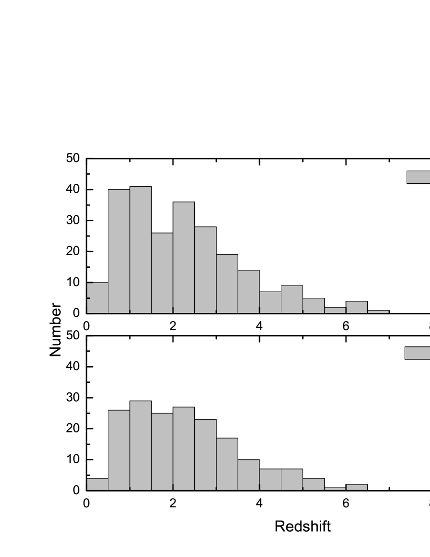
Figure 1: Top: The redshift distribution of the full GRB sample including 244 GRBs. Bottom: The reduced redshift distribution of 182 GRBs with redshifts obtained either from only afterglows, or from both afterglows and host galaxies.

Including long and short GRBs, Swift has detected more than 900 GRBs (until GRB 141026A) in the past 10 years. However, recent studies suggest that the classical classification of short and long GRBs with $T_{90}=2\,{\rm s}$ is not appropriate for Swift. Bromberg et al. (2013) argued that a more suitable selection for long GRBs from Swift satellite should be defined by $T_{90}>0.8\,{\rm s}$, which is based on a physically motivated model. Here we believe that the classification with $T_{90}=2\,{\rm s}$ is more strict in our study. As shown in Figure 3 of Bromberg et al. (2013), the probability of a GRB with $T_{90}>2\,{\rm s}$ to be a collapsar is more than $80\%$, which is higher than $50\%$ for $T_{90}>0.8\,{\rm s}$. Additionally, three sub-luminous GRBs (GRB 060218, 060505, 100316D) with luminosity $L<10^{49}\,{\rm erg}\,{\rm s}^{-1}$ have been excluded from our sample (Soderberg et al. 2006; Liang et al. 2007; Virgilii et al. 2008; Howell et al. 2011; Howell & Coward 2013), three ultra-long GRBs (GRB 101225A, 111209A, 121027A) have been suggested to be another population(Gendre et al. 2013; Stratta et al. 2013; Levan et al. 2014). We also exclude 22 possible short GRBs (GRB 050416A, 050724, 050911, 051016B, 051114, 051227, 060505, 060614, 061006, 061210, 070714B, 071227, 080123, 080503, 080520, 090531B, 090607, 090715B, 090916, 100213A, 100216A, 100816A; Dietz 2011; Kopač et al. 2012; Fong et al. 2013; Tsutsui et al. 2013; Howell & Coward 2013; Berger 2014; Howell et al. 2014).

In this paper, the redshift data was taken from the Swift archive . After removing the uncertain redshifts, we obtained 282 GRBs (including long and short GRBs) with measured redshifts, which is around 30% of the BAT-triggered GRBs. For long GRBs, their redshifts are always measured from afterglows and/or the host galaxies observed by the ground-based telescopes, including the Very Large Telescope (VLT), Gemini-S-N, Keck and Lick. Finally, we obtained 244 long GRBs with confirmed redshifts (the full redshift sample). However, this full redshift sample is greatly affected by the observation biases. On one hand, more low redshift GRBs could be observed, as the brightest GRBs are predominantly nearby. On the other hand, some redshift dependent selection effects even could change the shape of the redshift distribution. As shown in the upper panel of Figure 1, a large number of GRBs missed their redshifts in the range of $1.5<z<2$, which may caused by the “redshift desert” effect. Therefore, to derive a less biased redshift sample is an immediate necessity of this work. Following Fynbo et al. (2009), we reconstruct our redshift sample by considering redshifts measured either from afterglows, or from both afterglows and host galaxies. We exclude the bursts with redshifts measured from the emission spectra of the host galaxies, as these bursts always cover a low redshift range (e.g., $0.3<z<2.8$; Wanderman & Piran 2010, Howell et al. 2014). We also exclude GRBs with photometric redshifts because of the large uncertainties. After doing this, we obtained a less biased redshift sample with 182 GRBs (the reduced redshift sample). The distribution of the reduced redshift sample is shown in the bottom panel of Figure 1. It’s obvious that the completeness of the reduced redshift sample is better than that of the full redshift sample, as shown in the top and bottom panels of figure 1 (e.g., in the redshift range of $1.5<z<2$). However, one may argue that the missing redshifts of GRBs in the range of $1.5<z<2$ may be caused by the statistical fluctuations. For this point, we will discuss it in section 4.1.

In this work, we use the GRB peak flux data in the energy range of 15-150$\,{\rm keV}$ of the BAT. The data was taken from the Butler’s online catalogue, which is the extension of the work presented in Butler et al. (2007, 2010). As the peak flux data can be measured directly from BAT by assuming the fewest burst characters, we suggest that the peak flux distribution is the least uncertain property. Finally, we obtained a total number of 681 bursts with peak fluxes.

3 The model

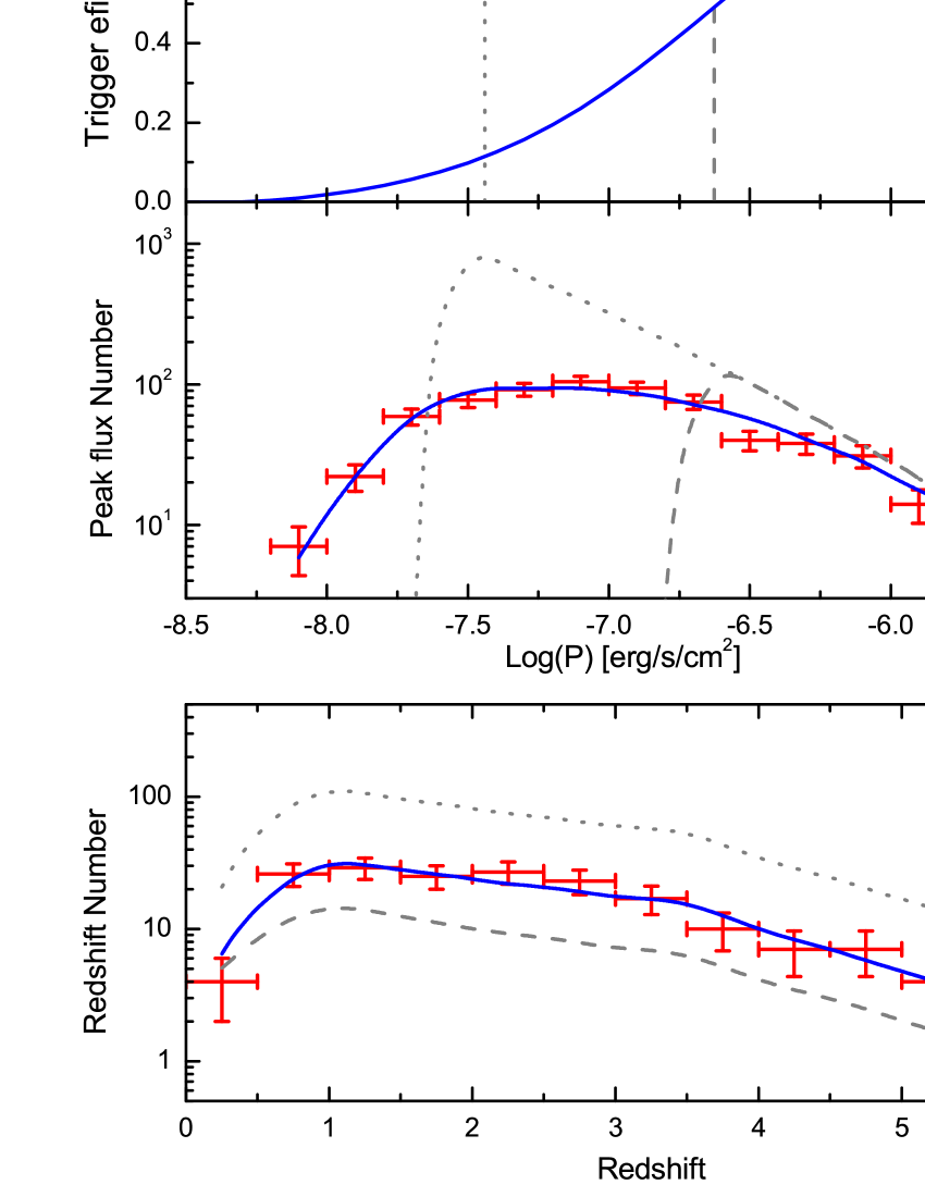
Figure 2: Top: The triggering efficiency of Swift as a function of peak flux (blue solid line), and the single detection threshold of 2.6 ph $\,{\rm s}^{-1}\,\rm cm^{-2}$ (gray dashed line) and 0.4 ph $\,{\rm s}^{-1}\,\rm cm^{-2}$ (gray dotted line). The middle and bottom figures show the effects of the triggering algorithm on the number distributions of peak flux and redshift (for RGRB1 for example), respectively.

The first step of our work is to fit the GRB number distributions of peak flux and redshift, which are both related to the GRB rate and LF. The expected number of GRBs with observed peak fluxes between $P_{1}$ and $P_{2}$ that triggered the BAT can be expressed by

$$N(P_{1},P_{2})={\Delta\Omega\over 4\pi}T\int^{\infty}_{0}\int^{L_{2}}_{L_{1}}\eta(P)\Phi_{z,P}(L)\dot{R}(z)dL{dV(z)\over 1+z},$$ (1)

where $(\Delta\Omega/4\pi)\sim 0.1$ is the field view of the BAT, $T\sim 10~{}\rm yrs$ is the observational period, $dV(z)$ is the comoving volume and $1/(1+z)$ accounts for the time dilation, $\eta(P)$ is the triggering function, $\Phi_{z,P}(L)$ is the LF with $L_{\min}=10^{49}\,{\rm erg}\,{\rm s}^{-1}$ and $L_{\max}=10^{57}\,{\rm erg}\,{\rm s}^{-1}$ for normalization, and $\dot{R}(z)$ is the GRB rate. The expected number of GRBs within redshift range of $z_{1}<z<z_{2}$ is given by

$$N(z_{1},z_{2})={\Delta\Omega\over 4\pi}T\int^{z_{2}}_{z_{1}}\int^{L_{\max}}_{L_{\rm min}}\eta(P)\Phi_{z,P}(L)\dot{R}(z)dL{dV(z)\over 1+z}.$$ (2)

For the flat $\Lambda$CDM cosmology, we employ the cosmological parameters from WMAP nine-year results with $\Omega_{m}=0.28,\Omega_{\Lambda}=0.72$ and $H_{0}=70\,{\rm km}\,{\rm s}^{-1}\,{\rm Mpc}^{-1}$.

The triggering algorithm of Swift is complicated. Lien et al. (2014) simulated 50,000 GRBs to mock the triggering efficiency, where GRB light curves, incident angles, BAT’s active detector number, and the image trigger algorithm are considered. Although a specific set of parameters are included, we consider that the triggering algorithm is better than other techniques. By comparing the simulated peak flux number distribution with the real triggered one, Howell et al. (2014) derived the flux triggering efficiency in a functional form of

$$\eta(P)={a(b+cP/P_{0})\over(1+P/dP_{0})},$$ (3)

with $P>5.5\times 10^{-9}\,{\rm erg}\,{\rm s}^{-1}\,\rm cm^{-2}$, and below this range the function equals to zero. The function parameters are as follows: a=0.47, b=-0.05, c=1.46, d=1.45 and $P_{0}=1.6\times 10^{-7}\,{\rm erg}\,{\rm s}^{-1}\,\rm cm^{-2}$ (Howell et al. 2014). We could reproduce the triggered GRB population in Lien et al (2014) by using this triggering function. It seems that the sample completeness is much better than that of the step function approximation. In figure 2, we compare $\eta(P)$ with two step function approximations, e.g., a value of 0.4 ph $\,{\rm s}^{-1}\,\rm cm^{-2}$ and a value of 2.6 ph $\,{\rm s}^{-1}\,\rm cm^{-2}$, which have been used by Salvaterra et al. (2012). From the middle panel of the figure, we see that the threshold of 0.4 ph $\,{\rm s}^{-1}\,\rm cm^{-2}$ predicts more dim GRBs, while the threshold of 2.6 ph $\,{\rm s}^{-1}\,\rm cm^{-2}$ predicts more bright ones. It is apparent that the adoption of such approximations could be problematic while estimating the relative contributions of bright and dim GRBs. Furthermore, it seems that the adoption of different triggering algorithms do not change the shape of the redshift distribution significantly, but change the GRB number greatly as shown in the bottom panel of the figure. So it is obvious that the threshold of 0.4 ph $\,{\rm s}^{-1}\,\rm cm^{-2}$ predicts a lower local GRB rate, while the threshold of 2.6 ph $\,{\rm s}^{-1}\,\rm cm^{-2}$ predicts a higher one.

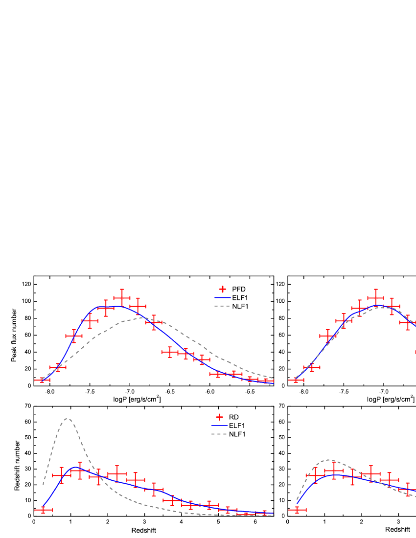
Figure 3: Left: The number of peak flux distribution (top; PFD) and redshift distribution (bottom; RD) of RGRB1. The solid blue lines are our best fitting results with an evolving LF (ELF1). The dashed gray lines are the fitting results with an non-evolving LF (NLF1). Right: The same as the left figures but for RGRB2.

The isotropic-equivalent peak luminosity in the source frame can be calculated by

$$L=4\pi d_{\rm L}(z)^{2}P{k(z)\over b},$$ (4)

where $P$ is the peak flux (in units of $\,{\rm erg}\,{\rm s}^{-1}\,\rm cm^{-2}$) in the observed energy band of $15-150\,{\rm keV}$, $d_{\rm L}(z)=(1+z)d_{c}(z)$ is the luminosity distance. The term ${k(z)/b}$ is to convert the observed energy band to the rest frame band of $1-10^{4}\,{\rm keV}$. Here $b$ accounts for the bolometric energy fraction that seen in the detector band (Wanderman & Piran 2010, Howell et al. 2011), and $k(z)$ is the cosmological correction. We express them in the form of

$$b=\int^{150}_{15}ES(E)dE/\int_{1}^{10^{4}}ES(E)dE$$ (5)

and

$$k(z)=\int^{150}_{15}ES(E)dE/\int_{15(1+z)}^{150(1+z)}ES(E)dE,$$ (6)

respectively. Here $S(E)$ is the rest frame photon spectrum, which can be well expressed by the empirical Band function (Band et al. 1993, 2003). The high and low energy spectral indices are given by -2.25 and -1, respectively. The spectral peak energy in the source frame can be derived by the Yonetoku relation (Yonetoku et al. 2004)

$$E_{p}(1+z)=\left({2.34\times 10^{47}\over L}\right)^{-1/2},$$ (7)

which is a much tighter and reliable relation.

We assume a broken power law form for the LF, which is suggested to be better than that of a single power law(e.g., Cao et al. 2011; Tan et al. 2013)

$$\Phi_{z,P}(L)\propto\left\{~{}\begin{array}[]{ll}\left({L\over L_{b}(z)}\right)^{-\alpha},{}{}{}{}&L\leq L_{b}(z),\\ \left({L\over L_{b}(z)}\right)^{-\beta},{}{}{}{}&L>L_{b}(z),\end{array}\right.,$$ (10)

where the break luminosity is assumed to evolve with redshift in the form of $L_{b}(z)=\mathcal{C}\times(1+z)^{\tau}$. The normalization coefficient is taken by assuming the minimum luminosity of $L_{\rm min}=10^{49}\,{\rm erg}\,{\rm s}^{-1}$. Here $\alpha$, $\beta$, $\tau$ and $\mathcal{C}$ are the free parameters which will be determinated in the following section.

Finally, we consider two kind of GRB rate models. For the first one, we consider that GRB rate follows the SFR (RGRB1 for short). The observational GRB production rate can be connected to star formation rate as

$$\dot{R}_{1}(z)=f_{b}f_{c}\dot{\rho}_{*}(z),$$ (11)

where $f_{b}=0.01$ is the beaming degree of GRB outflows and $f_{c}$ arises from the particularities of GRB progenitors (e.g., mass, metallicity, magnetic field, etc). We assume $f_{b}f_{c}$ does not evolve with redshift, and the redshift evolution effect between GRB rate and SFR mainly originates from the LF.

For the SFR $\dot{\rho}_{*}(z)$ , we describe it as (Hopkins & Beacom 2006)

$$\dot{\rho}_{*}(z)\propto\left\{~{}~{}\begin{array}[]{ll}(1+z)^{3.44},&~{}~{}~{}~{}z\leq 0.97,\\ (1+z)^{0},&~{}~{}~{}~{}0.97<z\leq 3.5,\\ (1+z)^{\kappa},&~{}~{}~{}~{}3.5<z,\end{array}\right.$$ (15)

with the local star formation rate $\dot{\rho}_{*}(0)=0.02\rm M_{\odot}yr^{-1}Mpc^{-3}$. Here we assume the high-redshift SFR ($z>3.5$) evolves in the form of a power law, which is still ambiguous. However, motivated by the shapes of the SFR at $z<3.5$ and also implied by some preliminary measurements (Bouwens et al. 2008, 2011; Ellis et al. 2012) and GRBs as well as their host galaxies (Yüksel et al. 2008; Kistler et al. 2009; Wang & Dai 2011; Elliott et al. 2012), the power low form of the SFR is considerable. For simplicity, we set a typical value of $\kappa=-3$ in the following calculation (e.g., Wang 2013).

The second GRB rate model (RGRB2 for short) is derived from the observed long GRBs. Following Wanderman & Piran (2010), we describe it in a functional form of

$$\dot{R}_{2}(z)=\dot{R}_{0}\left\{~{}~{}\begin{array}[]{ll}(1+z)^{v_{1}},&~{}~{}~{}~{}z\leq z_{*},\\ (1+z)^{v_{2}},&~{}~{}~{}~{}z_{*}<z,\\ \end{array}\right.$$ (18)

with typical values of $z_{*}=3.6,v_{1}=2.1$, and $v_{2}=-0.7$ based on the recent study (e.g., Howell et al. 2014). This form of GRB rate model is widely used in literature.

4 Results

In this section, we constrain the model parameters by jointly fitting the peak flux distribution (PFD) and redshift distribution (RD; the reduced redshift sample). As mention in the above section, two GRB rate models are considered. In each model, five free parameters are to be constrained: $\alpha$, $\beta$, $\tau$, $\mathcal{C}$, and $f_{c}$ (for RGRB1) or $\dot{R}_{0}$ (for RGRB2). In fact, $f_{c}$ or $\dot{R}_{0}$ can be easily derived by equating the model predicted peak flux number (equation 1) to the observed one (number of 681), if other four parameters are constrained. Other three parameters of $\alpha$, $\beta$ and $\mathcal{C}$ are mainly determinated by the PFD. The lower P-values of PFD fix the values of $\alpha$ and $\mathcal{C}$, and $\beta$ is mainly determined by the higher P-values. For the value of $\tau$, it is strongly dependent on the redshift evolution of RD.

Model	$\alpha$	$\beta$	$\tau$	$\mathcal{C}$	$f_{c}$	$\dot{R}(0)$	$\chi^{2}$	$Q$	$\chi_{\rm PFD}^{2}$	$Q_{\rm PFD}$	$\chi_{\rm RD}^{2}$	$Q_{\rm RD}$
				$10^{50}\,{\rm erg}\,{\rm s}^{-1}$	$10^{-6}\,{\rm M_{\odot}}^{-1}$	$\,{\rm yr}^{-1}\,{\rm Gpc}^{-3}$
ELF1	$0.3^{+0.11}_{-0.2}$	$1.9^{+0.05}_{-0.05}$	$3.5^{+0.4}_{-0.2}$	$0.33^{+0.1}_{-0.055}$	$4.34^{+0.6}_{-0.39}$	$0.86^{+0.11}_{-0.08}$	17.74	0.77	12.31	0.26	5.43	0.71
ELF2	$0.1^{+0.73}_{-0.1}$	$2.1^{+0.13}_{-0.03}$	$0.8^{+0.1}_{-0.08}$	$14^{+6}_{-6}$	$--$	$0.54^{+0.25}_{-0.07}$	23.63	0.42	16.43	0.09	7.20	0.51
NLF1	$0.1^{+0.1}_{-0.1}$	$1.7^{+0.05}_{-0.05}$	$0$	$3^{+0.5}_{-0.3}$	$6.9^{+0.2}_{-0.2}$	$1.36^{+0.04}_{-0.04}$	296.77	$\sim$0	197.33	$\sim$0	99.44	$\sim$0
NLF2	$0.1^{+0.13}_{-0.1}$	$2.4^{+0.12}_{-0.14}$	$0$	$39^{+5.6}_{-3.2}$	$--$	$0.66^{+0.06}_{-0.05}$	39.2	0.026	21.45	0.029	17.75	0.038

Table 1: The best-fit parameters for an evolving LF (ELF) and non-evolving LF (NLF) for RGRB1 and RGRB2 (with number 1 and 2 represent the two models), respectively. The statistical quality parameters of the models are shown in the last six columns.

Before the start of the work, we first set a primary constraint on the related parameters, e.g., $\alpha>0$, $\beta>0$, $L_{b}(0)>10^{49}\,{\rm erg}\,{\rm s}^{-1}$, $\tau>0$, and the local GRB rate $\dot{R}(0)\in[0,2]\,{\rm yr}^{-1}\,{\rm Gpc}^{-3}$ for both GRB rate models. Then, we give an arbitrary set of values for the five free parameters in the allowed ranges. For each set of the parameters, we calculate the $\chi^{2}$ values for both PFD ($\chi^{2}_{\rm PFD}$) and RD ($\chi^{2}_{\rm RD}$). The total $\chi^{2}$ is assumed to be the linear combination of $\chi^{2}_{\rm PFD}$ and $\chi^{2}_{\rm RD}$. The best fit parameters are derived by minimizing the global $\chi^{2}$. At last, we obtain the error bars for the five parameters by setting $\chi^{2}=\chi^{2}_{\min}+5.89$, which corresponds to the parameters within 68.3% confidence level. Table 1 gives the values of the fitted parameters for each model. The degrees of freedom (for the simultaneous fit) in Table 1 is 28 minus the number of parameters. The information about the quality of the fit for models is also given in the table. For each model, we show the total $\chi^{2}$ and the goodness-of-fit Q (the probability to find a new $\chi^{2}$ exceeding the current one).

In figure 3, we plot the observed and model-predicted PFD and RD. The left and right figures are the fitting results for RGRB1 and RGRB2, respectively. The solid lines are for models with the evolving LFs, while the dashed lines are for models without evolution. From this figure, we conclude our results as follows:

1. For both GRB rate models, the evolving LFs (ELF) fit well with both PFD and RD, while the non-evolving LFs (NLF) fit the data poorly, which can be inferred from the values of the $\chi^{2}$ and Q in Table 1. For RGRB1, the non-evolving LF (NLF1) model shows an excess of GRBs at high P and low redshift (left panels in figure 3). For RGRB2 (NLF2), it also shows the same tendency as RGRB1 (right panels in figure 3). Therefore, we suggest that the LF should evolve with redshift and rule out the non-evolving LF for both GRB rate models.

2. A non-negligible fraction of high-redshift GRBs may exist in the current Swift GRB sample. In our reduced redshift sample, the highest redshift is $z=6.32$ (GRB 140515A). By using the best fit parameters provided in Table 1, we find nearly 23 GRBs with their redshifts higher than 6.5 for RGRB1. Simulatively, nearly 24 GRBs with redshifts higher than 6.5 for RGRB2. However, the truth is that we only observed 4 GRBs with possible redshifts higher than that (GRB 060116, $z=4$ or 6.6; 080913, $z=6.44$ or $6.7$; 090423, $z=8.26$; 090429B,$z=9.3$). This result suggests that a large fraction of high-redshift GRBs (even with redshift higher than 10; e.g., Tan et al. 2015) may exist in the BAT-triggered GRB sample. Unfortunately, we can not measure their redshifts because of the instrumental reasons. It is also possible that these high-redshift GRBs may origin from Pop III stars (e.g., Mészáros & Rees 2010; Toma et al. 2011).

3. Except for the redshfit evolution of LF, an additional evolution may exist between the GRB rate and SFR. If the LF and GRB rate model of RGRB2 represent the intrinsic ones, the additional redshift evolution is obvious while comparing the values of $\tau$ between the two models ($\tau=3.5^{+0.4}_{-0.2}$ for RGRB1 and $\tau=0.8^{+0.1}_{-0.08}$ for RGRB2). However, it is hard to describe this evolution form as it may originate from many reasons, e.g., the evolution of cosmic metallicity (Wang & Dai 2009; Li 2008), initial mass function, different properties of progenitor, their host galaxies, or their combination. The collapsar model explains the formation of GRB via the collapse of a rapidly rotation massive iron core into a black hole (Woosley 1993). However, there are two basic problems of single-star model in producing collapsars. First, the spin-down of the stellar core due to core-envelope coupling. Second, the Wolf-Rayet winds can slow the rotation. Fortunately, the rapid rotation of low-metallicity stars can overcome both problems (Langer & Norman 2006). Such speculation is confirmed by observation (Fynbo et al. 2003; Modjaz et al. 2008; Graham & Fruchter 2013; Trenti et al. 2013; Wang & Dai 2014). So we believe that it is easier for low-metallicity stars to produce GRBs than the stars with high-metallicity. If we incorporate this effect into the LF (as we have done in the model of RGRB1, where only the redshift evolution of LF is considered, but ignore the evolution of the GRB progenitor properties), it will lead to a stronger redshift evolution of the LF, as the cosmic metallicity decreases with redshift. Futhermore, much more massive stars exist at high redshift, which will lead to more energetic GRBs and also increase the LF evolution. Therefore, the intrinsic redshift evolution of the LF should in the range of $0.8^{+0.1}_{-0.08}<\tau<3.5^{+0.4}_{-0.2}$ for reality.

4.1 Redshift selection effect

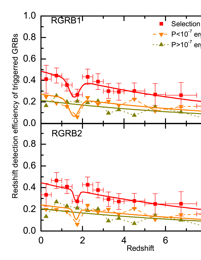
Figure 4: Redshift detection efficiency of BAT-triggered GRBs of Swift, with a total number of 244 GRBs with redshifts measured from afterglows and/or host galaxies. Top: Redshift detection efficiency for RGRB1. The solid squares correspond to the detection efficiency of the total GRBs. The up-triangles (down-triangles) with dotted (dashed) line correspond to the detection efficiency of GRBs with peak fluxes $>10^{-7}\,{\rm erg}\,{\rm s}^{-1}\,\rm cm^{-2}$ ($<10^{-7}\,{\rm erg}\,{\rm s}^{-1}\,\rm cm^{-2}$). The solid lines are our fitting results. Bottom: The same as that of the top panel, but for RGRB2.

There are two major elements to affect the GRB redshift detection efficiency: one is the instrumental bias and the other is the redshift-dependent selection effect. For the first point, the localization and sensitivity of the follow-up afterglow observations have great impact on the detection probability of GRB redshifts. The quick response and high sensitivity making Swift detect the largest number and the highest redshift of GRBs. Assuming GRB optical afterglows decrease like power laws with exponent $\gamma\sim-1$, Swift will detect GRB afterglows with 2.9 and 4.0 mag brighter than $HETE2$ and $BeppoSAX$ (Fiore et al. 2007), respectively. For the second point, the host galaxy dust obscuration plays a most important role in the measurement of GRB redshifts. It is suggested that a fraction of 30-35 percent of GRBs miss their redshifts for dust obscuration (Coward et al. 2013). In addition, the so-called “redshift desert” effect can also lead to a fraction of nearly $20\%$ of GRBs missing their redshifts in the range of $1.1<z<2.1$ (Steidel et al. 2005; Fiore et al. 2007; Coward et al. 2013). The Malmquist bias arises because of the sensitivity of telescopes and instruments, which leads to a decreasing redshift detection efficiency to higher redshift. Therefore, we only have $\sim 30\%$ of GRBs with measured redshifts.

In Figure 4, we compare the number distribution of the full redshift sample with our model predicted one in each redshift bin. The ratio could be considered as the redshift detection efficiency (solid squares). The error bars along the y-axis are the statistical errors (i.e., square root of the number in each bin $\Delta N=\sqrt{N}$), which correspond to the 68% Poisson confidence intervals for the binned events (Gehrels 1986). The x-axis error bars simply represent the bin size. For both GRB rate models, the detection efficiency have the tendency of decreasing with redshift. Particularly, nearly 20% of GRBs miss their redshifts in the range of $1<z<2.5$, which could be the evidence of the “redshift desert” effect. Furthermore, we divide the full redshift sample into two groups: one with peak fluxes $P>10^{-7}\,{\rm erg}/\,{\rm s}/\,\rm cm^{2}$ (up-triangles with dotted line), and the other with $P<10^{-7}\,{\rm erg}/\,{\rm s}/\,\rm cm^{2}$ (down-triangles with dashed line). It is obvious that the “redshift desert” effect mainly results from the low peak flux GRBs with $P<10^{-7}\,{\rm erg}/\,{\rm s}/\,\rm cm^{2}$. For GRBs with $P>10^{-7}\,{\rm erg}/\,{\rm s}/\,\rm cm^{2}$, the detection efficiency just decreases with redshift and has no relation with the “redshift desert” effect. See from the figure, we could find more high (or less low) redshift GRBs at low (high) peak fluxes, which may also indicate that high (low) redshift GRBs always have low (high) peak fluxes. For simplicity, we first fit the detection efficiency of RGRB1 with an exponential function multiple a Gauss function as

$$\eta_{\rm t}(z)=0.36\times e^{0.3-z/8.9}\times(1-0.41\times e^{-(z-1.6)^{2}/0.11}).$$ (19)

Then we fit the sample with $P>10^{-7}\,{\rm erg}/\,{\rm s}/\,\rm cm^{2}$ by multiplying an constant with equation (12) but without the Gauss fraction, and the fitting result could be expressed as

$$\eta_{\rm h}(z)=0.16\times e^{0.3-z/8.9}.$$ (20)

For the detection efficiency of $P<10^{-7}\,{\rm erg}/\,{\rm s}/\,\rm cm^{2}$, we obtain it by subtracting equation (13) from (12), which is $\eta_{\rm l}(z)=\eta_{\rm t}(z)-\eta_{\rm h}(z)$. It seems that $\eta_{\rm l}(z)$ also fits the reuslt quite well, which could also support our result that the “redshift desert” effect mainly comes from low flux GRBs. For RGRB2 model, we go through the same steps and the fitting results are as follows,

$$\eta_{\rm t}^{\prime}(z)=0.33\times e^{0.3-z/9.6}\times(1-0.3\times e^{-(z-1.7)^{2}/0.02})$$ (21)

and

$$\eta_{\rm h}^{\prime}(z)=0.15\times e^{0.3-z/9.6}.$$ (22)

Finally, we obtain $\eta_{\rm l}^{\prime}(z)=\eta_{\rm t}^{\prime}(z)-\eta_{\rm h}^{\prime}(z)$, which also fits the observation quit well. The fitting results are shown as the solid lines in Figure 4. The goodness of the fits at the highest redshift are greatly affected by the GRB number. Here we should mention that the “redshift desert” effect exists in both GRB rate models, particularly in the dimmer GRB sample. However, if this is caused by the statistical fluctuations, the “redshift desert” effect will disappear. Then, the redshift detection efficiency will be nearly a constant at $z<2.5$ and decrease at higher redshift. The problem is that the fluctuations only exist in the dimmer GRBs, but not in both dimmer and brighter GRB samples. The so-called “redshift desert” is a redshift region ($1<z<2.1$) where it is difficult to measure absorption and emission spectra of the sources. As redshift increases beyond $z\sim 1$, the strong emission lines from the host galaxies (e.g. the [O III]$\lambda\lambda$4959, 5007, [O II]$\lambda$3727 line, H$\alpha$, H$\beta$) are shifted outside of the typical interval covered by optical spectrometers ($\approx 3800-8000{\AA}$) at $z>1$, while Lyman-$\alpha$ enters the range at $z\sim 2.1$. This becomes more serious for faint sources, as the spectra of the faint sources always have small signal to noise ratio. Therefore, we believe that dimmer GRBs are more responsible for the “redshift desert” effect, which can not be caused by the statistical fluctuations.

5 Summary and discussion

In this work, we utilized both the peak flux and redshift distributions to constrain the LF. We don’t use the pseudo redshifts inferred from the empirical luminosity relations, because these relations could be greatly affected by the observational bias, e.g., trigger efficiency (Shahmoradi & Nemiroff 2011). By jointly fitting the PFD and RD, we found that the non-evolving LF fits the data poorly, while the evolving LF fits data well. The evolution of the break luminosity can be expressed as $L_{b}\propto(1+z)^{\tau}$, with $\tau=3.5^{+0.4}_{-0.2}$ and $\tau=0.8^{+0.1}_{-0.08}$ for RGRB1 and RGRB2, respectively. The strong and weak redshift evolution of the LFs for two GRB rate models might imply an additional redshift evolution between GRB rate and SFR. The strong redshift evolution of LF for RGRB1 is based on the assumption that only LF evolves with redshift, which is not real if GRB progenitors evolve with redshift. If we take these effects into account, the redshift evolution of the LF may become weaker for RGRB1 (e.g., $\tau<3.5^{+0.4}_{-0.2}$). However, it is impossible to distinguish this additional evolution under the current situation, unless the number of GRBs with measured redshifts is large enough to satisfy the LF fittings in different redshift ranges (Tan et al. 2013).

The local GRB rates are $\dot{R}(0)_{1}=0.86^{+0.11}_{-0.08}\,{\rm yr}^{-1}\,{\rm Gpc}^{-3}$ and $\dot{R}(0)_{2}=0.54^{+0.25}_{-0.07}\,{\rm yr}^{-1}\,{\rm Gpc}^{-3}$ for RGRB1 and RGRB2, respectively, which are consistent with the previous works (e.g., Schmidt 1999, 2001; Guetta et al. 2004, 2005; Liang et al. 2007; Wanderman & Piran 2010; Cao et al. 2011; Lien et al. 2014). Furthermore, we suggest that a large fraction of high-redshift GRBs ($z>6.5$) may have been detected by Swift satellite but without measured redshifts. These high-redshift GRBs may be produced by Pop III stars (e.g., Mészáros & Rees 2010; Toma et al. 2011; Tan et al. 2015).

To reduce the large biases introduced by the complex triggering criterion of Swift, we use the recent peak flux efficiency function for the triggering criterion instead of the constant photon flux (Howell et al. 2014). The constant photon flux triggering criterion could be problematic while estimating the contribution of the dim and bright GRBs as shown in figure 2. The introduction of a dependence of $L$ on $E_{p}$ has little effect on our results, and the Yonetoku relation is considered to be tight enough.

To reduce the redshift selection effect, only GRBs with redshifts measured from afterglows or from both afterglows and host galaxies are considered. After deriving the best-fit parameters, we compare the observed full redshift distribution with our model predicted one. Our results show that the redshift detection efficiency decreases with redshift slowly in general, and nearly 20% of GRBs missed their redshifts in the “redshift desert” range of $1<z<2.5$. The reason for the slow decreasing tendency of the detection efficiency might be the combined effects of the dust extinction and Malmquist bias, as the higher (lower) redshift GRBs always have less (more) dust contents but lower (higher) peak fluxes (e.g. Bouwens et al. 2009; Perley et al. 2009; Zafar et al. 2011; Rossi et al. 2012). By dividing the GRB sample into the dim and bright groups, we find that the “redshift desert” effect is mainly introduced by the low-flux GRBs, which is a useful result for the completeness of the sample selection in future works.

References

- (1) Band D., Matteson, J., Ford, L., et al., 1993, ApJ, 413, 281
- (2) Band D., 2003, ApJ, 588, 945
- (3) Band D. L., 2006, ApJ, 644, 378
- (4) Berger E., Chornock R., Holmes T. R., et al., 2011, ApJ, 743, 204
- (5) Berger E., 2014, ARA&A, 52, 43
- (6) Bloom J. S., Kulkarni S. R., Price P. A., et al., 2002, ApJL, 572, L45
- (7) Bouwens R. J., et al., 2008, ApJ, 686, 230
- (8) Bouwens R. J., et al., 2011, Natur, 469, 504
- (9) Bouwens R. J., et al., 2009, ApJ, 705, 936
- (10) Bromberg O., et al., 2013, ApJ, 764, 179
- (11) Butler N. R., Kocevski D., Bloom J. S., Curtis J. L., 2007, ApJ, 671, 656
- (12) Butler N. R., Bloom J. S., Poznanski D., 2010, ApJ, 711, 495
- (13) Campana S., Mangano V., Blustin A. J., et al., 2006, Natur, 442, 1008
- (14) Cao X. F., Yu Y. W., Cheng K. S., Zheng X. P., 2011, MNRAS, 416, 2174
- (15) Chary R., Berger E., Cowie L., 2007, ApJ, 671, 272
- (16) Cheng K. S., Yu Y. W., Harko T., PRL, 104, 241102
- (17) Cucchiara A., et al., 2011, ApJ, 736, 7
- (18) Coward D. M., Burman R. R., 2005, MNRAS, 361, 362
- (19) Coward D. M., et al., 2013, MNRAS, 432, 2141
- (20) Dietz A., 2011, A&A, 529, A97
- (21) Eichler D., Livio M., Piran T., & Schramm D. N., 1989, Natur, 340, 126
- (22) Ellis R. S., et al., 2012, arXiv: 1211.6804
- (23) Elliott J., Greiner J., Khochfar S., et al., 2012, A&A, 539, A113
- (24) Fiore F., et al., 2007, A&A, 470,515
- (25) Firmani C., Avila-Reese V., Ghisellini G., Tutukov A. V., 2004, ApJ, 611, 1033
- (26) Fong W., Berger E., Chornock R., et al., 2013, ApJ, 769, 56
- (27) Fynbo, J. P. U., et al. 2003, A&A, 406, L63
- (28) Fynbo J. P. U., Jakobsson P., Prochaska J. X., et al., 2009, ApJS, 185, 526
- (29) Galama T. J., Vreeswijk P. M., van Paradijs J., et al., 1998, Natur, 395, 670
- (30) Gehrels, N. 1986, ApJ, 303, 336
- (31) Gendre B., et al., 2013, ApJ, 766, 30
- (32) Graham, J. F., & Fruchter, A. S. 2013, ApJ, 774, 119
- (33) Greiner J., et al., 2009, ApJ, 693, 1610
- (34) Hopkins, A. M., & Beacom, J. F. 2006, ApJ, 651, 142
- (35) Howell E. J., et al., 2007, ApJL, 666, L65
- (36) Howell E. J., et al., 2011, MNRAS, 410, 2123
- (37) Howell E. J., Coward D. M., 2013, MNRAS, 428, 167
- (38) Howell E. J., et al., 2014, MNRAS, 444,15
- (39) Kistler M. D., et al., 2008, ApJL, 673, L119
- (40) Kistler M. D., Yüksel H., Beacom J. F., et al., 2009, ApJL, 705, L104
- (41) Kocevski D., Liang E. W., 2006, ApJ, 642, 371
- (42) Kopač D., et al., 2012, MNRAS, 424, 2393
- (43) Langer L., Norman C. A., 2006, ApJL, 638, L63
- (44) Le T., Dermer C. D., 2007, ApJ, 661, 394
- (45) Levan A. J., et al., 2014, ApJ, 781, 13
- (46) Li L. X., 2008, MNRAS, 388, 1487
- (47) Liang, E. W., Zhang, B., Virgili, F., & Dai, Z. G. 2007, ApJ, 662, 1111
- (48) Lien A., Sakamoto T., Gehrels N., Palmer D. M., et al., 2014, ApJ, 783, 24
- (49) Lloyd-Ronning N. M., Fryer C. L., Ramirez-Ruiz E., 2002, ApJ, 574, 554
- (50) Matsubayashi T., Yamazaki R., Yonetoku D., et al., 2005, Prog. Theor. Phys., 114, 983
- (51) Mészáros P., Rees M. J., 2010, ApJ, 715, 967
- (52) Melandri A., Pian E., Ferrero P., et al., 2012, A&A, 547, A82
- (53) Modjaz, M., et al. 2008, AJ, 135, 1136
- (54) Nakar E., 2007, PhR, 442, 166
- (55) Paczyński B., 1998, ApJL, 494, L45
- (56) Perley D. A., et al., 2009, AJ, 138, 1690
- (57) Petrosian V., et al., 2015, arXiv:1504.01414
- (58) Porciani C., Madau P., 2001, ApJ, 548, 522
- (59) Robertson B. E., Ellis R. S., 2012, ApJ, 744, 95
- (60) Rossi A. et al., 2012, A&A, 545, A77
- (61) Salvaterra R. et al., 2012, ApJ, 749, 68
- (62) Schmidt M., 1999, ApJL, 523, L117
- (63) Schmidt M., 2001, ApJL, 559, L79
- (64) Shahmoradi A., Nemiroff R. J., 2011, MNRAS, 411, 1843
- (65) Soderberg A. M. et al., 2006, Natur, 442, 1014
- (66) Stanek K. Z., Matheson T., Garnavich P. M., et al., 2003, ApJL, 591, L17
- (67) Steidel C., Shapley A., Pettini M., Adelberger K., Erb D., Reddy N., Hunt M., 2005, eds, Proc. ESO Workshop, Multi-wavelength Mapping of Galaxy Formation and Evolution, Springer, Berlin, p. 169
- (68) Stratta G., et al., 2013, ApJ, 779, 66
- (69) Tan W. W., Cao X. F., Yu, Y. W., 2013, ApJL, 772, L8
- (70) Tan W. W., Cao X. F., Yu, Y. W., 2015, New Astronomy, 38, 11
- (71) Thomsen B., Hjorth J., Watson D., et al., 2004, A&A, 419, L21
- (72) Toma K., Sakamoto, T., Mészáros P., 2011, ApJ, 731, 127
- (73) Totani T., 1997, ApJL, 486, L71
- (74) Trenti, M., Perna, R. & Tacchella, S., 2013, ApJ, 773, L22
- (75) Tsutsui R., et al., 2013, MNRAS, 431, 1398
- (76) Virgilii F. J., Liang E.-W., Zhang B., 2008, MNRAS, 392, 91
- (77) Wanderman D., Piran T., MNRAS, 2010, 406, 1944
- (78) Wang F. Y., Dai Z. G., 2009, MNRAS, 400, L10
- (79) Wang F. Y., Dai Z. G., 2011, ApJL, 727, L34
- (80) Wang F. Y., Dai Z. G., 2014, ApJS, 213, 15
- (81) Wang F. Y., 2013, A&A, 556, A90
- (82) Wang F. Y., Dai Z. G., Liang E. W., 2015, New, Astro. Rev., 67, 1
- (83) Wijers R. A. M. J., Bloom J. S., Bagla J. S., Natarajan P., 1998, MNRAS, 294, L13
- (84) Woosley, S. E. 1993, ApJ, 405, 273
- (85) Yonetoku D., Murakami T., Nakamura T., et al., 2004, ApJ, 609, 935
- (86) Yu H., Wang F. Y., Dai Z. G., Cheng K. S., 2015, ApJS, 218, 13
- (87) Yüksel H., et al., 2008, ApJL, 683, L5
- (88) Zafar T., et al., 2011, ApJ, 735, 2