An $H_{\infty}$ Cooperative Fault Recovery Control of Multi-Agent Systems

Abstract

In this work, an $H_{\infty}$ performance fault recovery control problem for a team of multi-agent systems that is subject to actuator faults is studied. Our main objective is to design a distributed control reconfiguration strategy such that a) in absence of disturbances the state consensus errors either remain bounded or converge to zero asymptotically, b) in presence of actuator fault the output of the faulty system behaves exactly the same as that of the healthy system, and c) the specified $H_{\infty}$ performance bound is guaranteed to be minimized in presence of bounded energy disturbances. The gains of the reconfigured control laws are selected first by employing a geometric approach where a set of controllers guarantees that the output of the faulty agent imitates that of the healthy agent and the consensus achievement objectives are satisfied. Next, the remaining degrees of freedom in the selection of the control law gains are used to minimize the bound on a specified $H_{\infty}$ performance index. The effects of uncertainties and imperfections in the FDI module decision in correctly estimating the fault severity as well as delays in invoking the reconfigured control laws are investigated and a bound on the maximum tolerable estimation uncertainties and time delays are obtained. Our proposed distributed and cooperative control recovery approach is applied to a team of five autonomous underwater vehicles to demonstrate its capabilities and effectiveness in accomplishing the overall team requirements subject to various actuator faults, delays in invoking the recovery control, fault estimation and isolation imperfections and unreliabilities under different control recovery scenarios.

I Introduction

Utilization of unmanned vehicles (agents) in operations where human involvement is dangerous, or impossible as in deploying mobile robots for planetary surface exploration, autonomous underwater vehicles for surveying deep sea, among others, has recently received extensive interest by the research community. In addition, deployment of multiple vehicles such as spacecraft, mobile robots, or unmanned underwater vehicles instead of using a single vehicle increases the system performance and reliability, while it will ultimately reduce the cost of the overall mission.

In safety critical missions, the agents should have the capability to cope with unexpected external influences such as environmental changes or internal events such as actuator and sensor faults. If these unexpected events are not managed successfully, they can lead to the team instability or cause sever overall team performance degradations. For example, the crash of the NASA’s DART spacecraft in 2006 was due to a fault in its position sensors [6].

The development of control reconfiguration for multi-agent systems is distinct from the control design problem of healthy multi-agent systems [4, 23, 28, 21]. This is so in the sense that the former should be ideally solved on-line and use only local information given that faults occur at unknown times, have unknown patterns, and the existing fault detection and isolation (FDI) module in the team information may be available only locally, while the latter problem can be solved off-line and by potentially using the entire system information. Moreover, due to the information sharing structure of multi-agent systems, the fault tolerant control approaches that have extensively been studied in the literature for single agent systems [Yang2010, 30, 16, 22, 14] will not be directly applicable to multi-agent systems.

Recently, the control reconfiguration problem of multi-agent systems has been studied in [25, 1, 9, 10, 33, 32, 5, 27, 26, 20, 19, 13, 29]. In [25, 1], formation flight problem in a network subject to loss of effectiveness (LOE) faults is considered and in [9, 10, 33] the consensus achievement problem in faulty multi-agent systems is studied. In [25], a discrete-event supervisory module is designed to recover the faults that cannot be recovered by the agents using only local recovery solutions. In [1], a high-level performance monitoring module is designed that monitors all the agents and detects deviations of the error signals from their acceptable ranges. This module would then activate a high-level supervisor to compensate for the deviations in the performance specifications due to limitations of the low-level recovery strategy. In [32, 5, 27, 26] adaptive control approaches are employed to compensate for actuator faults and in [20, 19] control reconfiguration problem in a team of Euler Lagrange systems subject to actuator faults and environmental disturbances is studied. Finally in [13, 29], attitude synchronization problem for a team of satellites in presence of actuator faults is studied.

In this work, $H_{\infty}$ performance control reconfiguration problem in multi-agent systems subject to occurrence of three types of faults, namely, the loss of effectiveness (LOE), stuck and outage faults is studied. The proposed $H_{\infty}$-based control reconfiguration strategy guarantees that the faulty agent outputs imitate those of the healthy system while the state consensus errors are either ensured to be asymptotically stable or remain bounded in absence of disturbances and the disturbance attenuation bound is minimized when the disturbances exist. Furthermore, this approach can compensate for the outage and stuck faults which cause rank deficiency and change the agent structure, whereas in the adaptive approaches it is assumed that the fault does not cause rank deficiency.

Our proposed approach is similar to the works in [33, 10], but it has the following distinctions, namely: (i) in [33] it is assumed that all the followers have access to the leader input signal while in this work we do not require this assumption, (ii) in [33] environmental disturbances have not been considered whereas in this work we do include disturbances in our analysis and design, (iii) in this work agents could be subject to simultaneous LOE, outage and stuck faults, however in [10] only a single LOE fault has been studied and in [33] only LOE and outage faults have been considered, (iv) in both [33, 10] the network topology is assumed to be indirected whereas in this work we have considered a directed network topology, and (v) in this work we ensure that the outputs of the faulty agent are exactly forced to follows those of the healthy agent and the state consensus errors remain bounded, whereas in [33, 10] the consensus problem is considered. The main motivation for enforcing outputs of the agents outputs to follow that of the leader is that in some applications like small light weight under vehicles, a small deviation in the speed can cause a big deviation in the agent position which may cause the network become disconnected or the agent becomes lost. In order to reach this objective, we formulated the problem as disturbance decoupling problem with stability and we use the Geometric approach [3] and controlled invariant subspaces to solve the problem along with linear algebra and matrix theory to address exact output following and state consensus error stability in the team as well as disturbance attenuation. To the best of our knowledge this problem has not been considered in the current literature in multi-agent systems.

In view of the above discussion, the main contributions of this work can be summarized as follows:

1. A distributed control reconfiguration strategies for multi-agent systems subject to LOE, outage and stuck faults are proposed and developed. Towards this end, associated with each agent a novel “virtual auxiliary system” is constructed for the first time in the literature. Each agent will receive information from only the states of its associated auxiliary agent and the nearest neighboring auxiliary agents. This is in contrast with conventional cooperative schemes where each agent will be receiving the actual state information from its nearest neighboring agents. The proposed strategy guarantee an $H_{\infty}$ performance control reconfiguration with stability.

2. The proposed reconfiguration control laws guarantee that the output of the faulty agent behaves the same as that of the healthy system, and moreover a specified $H_{\infty}$ performance index is minimized in presence of environmental disturbances.

3. The effects of uncertainties and imperfections in the FDI module decision in correctly estimating the fault severity as well as delays in invoking the reconfigured control laws are investigated and a bound on the maximum tolerable estimation uncertainties and time delays are obtained.

4. The proposed distributed reconfiguration control laws are capable of and designed specifically for accommodating single, concurrent and simultaneous actuator faults in multi-agent systems.

The remainder of this work is as follows. In Section II, the required background information are provided and the problem is formally defined. In Section III, the proposed reconfigured control law and the effects of uncertainties on the proposed solution are investigated. In Section IV, the proposed control laws are applied to a network of Autonomous Underwater Vehicles (AUV)s and extensive simulation results and various case studies are studied and presented. Finally, Section V concludes the paper.

II Background and Problem Definition

II-A Graph Theory

The communication network among $N+1$ agents can be represented by a graph. A directed graph $\mathcal{G}=(\mathcal{V},\mathcal{E})$ consists of a nonempty finite set of vertices $\mathcal{V}=\{v_{0},v_{1},...,v_{N}\}$ and a finite set of arcs $\mathcal{E}\subset\mathcal{V}\times\mathcal{V}$. The $i$-th vertex represents the $i$-th agent and the directed edge from $i$ to $j$ is denoted as the ordered pair $(i,j)\in\mathcal{E}$, which implies that agent $j$ receives information from agent $i$. The neighbor set of the $i$-th agent in the network is denoted by ${\mathcal{N}}_{i}=\{j|(j,i)\in\mathcal{E}\}$. The adjacency matrix of the graph $\mathcal{G}$ is given by $G=[g_{ij}]\in\mathbb{R}^{(N+1)\times(N+1)}$, where $g_{ij}=1$ if $j\in{\mathcal{N}}_{i}$, otherwise $g_{ij}=0$. The Laplacian matrix for the graph $\mathcal{G}$ is defined as $L=D-G$, where $D=\text{diag}\{d_{i}\}$ and $d_{i}=\sum_{j=0}^{N}{g_{ij}}$.

II-B Leader-Follower Consensus Problem in a Network of Multi-Agent Systems

The main objective of the consensus problem in a leader-follower (LF) network architecture is to ensure all the team members follow the leader’s specified trajectory/states. Consider a network with $N$ follower agents that are governed by

$$\dot{x}_{i}(t)=Ax_{i}(t)+Bu_{i}(t)+B_{\omega}\omega_{i}(t),\ x_{i}(t_{0})=x_{i0},\ i=1,..,N,$$ (1)

$$y_{i}(t)=Cx_{i}(t),$$

and a leader agent that has the dynamics given by

$$\dot{x}_{0}(t)=Ax_{0}(t)+Bu_{0}(t)+B_{\omega}\omega_{0}(t),$$ (2)

$$y_{0}(t)=Cx_{0}(t),$$

where matrices $A$, $B$, $C$, $B_{\omega}$ represent the agents dynamics matrices and are known, $x_{i}(t)\in\mathbb{R}^{n}$, $y_{i}(t)\in\mathbb{R}^{q}$, $u_{i}(t)\in\mathbb{R}^{m}$, and $\omega_{i}(t)\in\mathbb{R}^{p}$, $i=0,\dots,N$ are the agents states, outputs, control signals, and exogenous disturbance inputs. In this work, bounded energy disturbances are considered, i.e. $\omega_{i}(t)\in\mathcal{L}_{2}$, $i=0,\dots,N$ ($\omega_{i}(t)$ belongs to $\mathcal{L}_{2}$ if $\int_{t_{0}}^{\infty}\omega_{i}^{\text{T}}(t)\omega_{i}(t)\text{d}t\leq\infty$).

In the architecture considered in this paper, certain and a very few of the followers, that are designated as pinned agents, are communicating with the leader and receive data from it directly. The other followers are not in communication with the leader and exchange information only with their own nearest neighbor follower agents. On the other word, each agent only communicate with its neighbors and at least one agent is a neighbour of the leader. The consensus error signal for the $i$-th follower is now defined by

$$e_{i}(t) = g_{i0}(x_{i}(t)-x_{0}(t))+\sum_{j\in{\mathcal{N}_{i}}}(x_{i}(t)-x_{j}(t)),$$ (3)

where $g_{i0}=1$ if agent $i$ is a pinned agent or is directly communicating with the leader and is zero otherwise. When there are no environmental disturbances, i.e. $\omega_{i}(t)\equiv 0$, $t>0$, $i=0,\dots,N$ the team reaches a consensus if $e_{i}(t)$ converges to origin asymptotically as $t\to\infty$. However, when there exist environmental disturbances, $e_{i}(t)$ cannot converge to origin, although it should remain in a bounded region around the origin. We refer and designate both of these cases as achieving consensus through out this paper.

Based on the above representation for the network, the aim is that all follower agents follow the leader agent trajectory. Accordingly, we partition the network Laplacian matrix defined in Subsection II-A, as $L=\begin{bmatrix}L_{11}&L_{12}\\ L_{21}&L_{22}\end{bmatrix}$, $L_{11}=0$, $L_{21}=0$, where $L_{21}$ is a $N\times 1$ vector and represents the leader’s links to the followers and $L_{22}$ is an $N\times N$ matrix and specifies the followers’ connections. This will help us to discuss the effects of the leader agent and follower agents to reach the entire team objectives.

II-C The Types and Description of the Actuator Faults

Before formally defining the three fault types that are considered in this work, we let $B=\begin{bmatrix}b^{1},b^{2},\dots,b^{m}\end{bmatrix}$ denote the matrix of input channels of the healthy agent, where $b^{k}$ denotes the $k$-th column of the matrix $B$, $B^{fk}$ denote the matrix of the faulty agent with a fault in only the $k$-th input channel, and $B^{f}$ denote the matrix of the faulty agent subject to several concurrent faulty channels.
Loss of Effectiveness (LOE) Fault: For the LOE fault, only a percentage of the generated control effort is available to the agent for actuation, therefore the dynamics of the $i$-th faulty agent after the occurrence of a fault at $t=t_{f}$ is modelled according to

$$\dot{x}_{i}^{f}(t)=Ax_{i}^{f}(t)+B^{f}u_{i}(t)+B_{\omega}\omega_{i}(t),\ t\geq t_{f},\ i=1,\dots,N,$$ (4)

$$y_{i}^{f}(t)=Cx_{i}^{f}(t),$$

where $x_{i}^{f}(t)\in\mathbb{R}^{n}$ denotes the state of the faulty agent, $B^{f}=B\Gamma_{i}$, $\Gamma_{i}=\operatorname{diag}\{\Gamma_{i}^{k}\}$, for $k=1,\dots,m$, $\Gamma_{i}^{k}$ represents the fault effectiveness of the $k$-th channel of the $i$-th agent, $0<\Gamma_{i}^{k}<1$ if the $k$-th actuator is faulty, and $\Gamma_{i}^{k}=1$ if it is healthy.

Outage Fault: If the $k$-th actuator of the $i$-th agent is completely lost at the time $t=t_{f}$, then we have $u_{i}^{k}(t)=0$ for $t\geq t_{f}$, where $u_{i}(t)=\begin{bmatrix}u_{i}^{1}(t),\dots,u_{i}^{m}(t)\end{bmatrix}^{\text{T}}$. The dynamics of the $i$-th agent with an outage fault in its $k$-th actuator can be represented by

$$\dot{x}_{i}^{f}(t)=Ax_{i}^{f}(t)+B^{fk}u_{i}(t)+B_{\omega}\omega_{i}(t),\ t\geq t_{f},\ i=1,\dots,N,$$ (5)

$$y_{i}^{f}(t)=Cx_{i}^{f}(t),$$

where $B^{fk}=\begin{bmatrix}b^{1},b^{2},\dots,b^{k-1},0,b^{k+1},\dots,b^{m}\end{bmatrix}$.

Stuck Fault: If at the time $t=t_{f}$ the $k$-th actuator of the $i$-th agent freezes at a certain value and does not respond to subsequent commands, the fault is then designated as the stuck fault. The dynamics of the $i$-th faulty agent under this fault type can be modelled as

$$\dot{x}_{i}^{f}(t)=Ax_{i}^{f}(t)+Bu_{i}^{f}(t)+B_{\omega}\omega_{i}(t),\ t\geq t_{f},\ i=1,\dots,N,$$ (6)

$$y_{i}^{f}(t)=Cx_{i}^{f}(t),$$

where $u_{i}^{f}(t)=\begin{bmatrix}u_{i}^{1}(t),\dots,u_{i}^{k-1}(t),\underline{u}_{i}^{k},u_{i}^{k+1}(t),\dots,u_{i}^{m}(t)\end{bmatrix}^{\text{T}}$, and $\underline{u}_{i}^{k}=u_{i}^{k}(t_{f})$ for all $t\geq t_{f}$ denotes the value of the stuck command.

We are now in a position to state the following assumptions.

Assumption 1.

(a) The network graph is directed and has a spanning tree, and (b) The leader control input is bounded and the upper bound is known.

Assumption 2.

(a) The agents are stabilizable and remain stabilizable even after the fault occurrence.
(b) Each agent is equipped with a local FDI module which detects with possible delays and correctly isolates the fault in the agent and also estimates the severity of the fault with possible errors in the case of the LOE or stuck faults.

Regarding the above assumptions the following clarifications are in order. First, the Assumptions 1-(a) and 2-(a) are quite common for consensus achievement and fault recovery control design problems, respectively. Second, it is quite necessary that in most practical applications one considers a leader whose states are ensured to be bounded. Moreover, in practical scenarios the actuators are quite well understood and described and their maximum deliverable control effort and bound they can tolerate are readily available and known. Therefore Assumptions 1-(b) is also not restrictive. Furthermore, in Subsection III-B we analyze the system behavior for situations where either Assumption 2-(c) does not hold or the estimated fault severities by the FDI module are not accurate. We obtain the maximum uncertainty bound that our proposed approaches can tolerate. However, as stated in Assumption 2-(b), we require the correct actuator location as well as the type of the fault for guaranteeing that our proposed reconfigured control laws will yield the desired design specifications and requirements. The Scenario $4$ in Section IV does demonstrate the consequences of violating this assumption.

As far as Assumption 2-(c) is concerned, it should be noted that this assumption is indeed quite realistic for the following observations and justications. The transient time that any cooperative or consensus-based controller takes to settle down and the overall team objectives are satisfied is among one of the design consideration and specification for the controller selection. In most practical consensus achievement scenarios dealing with a healthy team, the transient time associated with the agent response is ensured to be settled down in a very small fraction of the entire mission time, and in most cases the healthy transient time takes a few seconds to minutes to die out. Therefore, it is quite realistic and indeed practical that during this very short and initial operation of the system, the agents are assumed to be fault free. In other words, we will not initiate the mission with agents that are faulty from the outset. It is highly unlikely that during the very first few moments after the initiation of the mission a fault occurs in the agents. For all the above explanations and observations we believe that Assumption 2-(c) is meaningful and quite realistic.

II-D Notations and Preliminaries

For a vector $x=\left[x_{1},\dots,x_{n}\right]^{\text{T}}$ we define $L^{1}$, $L^{2}$ (Euclidean norm ) and $L^{\infty}$ norm as $\|x\|_{1}=\sum_{i=1}^{n}|x_{i}|$, $\|x\|_{2}=\sqrt{x_{1}^{2}+\dots+x_{n}^{2}}$, $\|x\|_{\infty}=\max(|x_{1}|,\dots,|x_{n}|)$. The signal $x(t)$ is also represented as $x(t)=\text{col}\{x_{i}(t)\}$. The function $\text{sgn}\{x(t)\}$ is defined as

$$\text{sgn}\{x(t)\}=\begin{bmatrix}\text{sgn}\{x_{1}(t)\},\dots,\text{sgn}\{x_{n}(t)\}\end{bmatrix}^{\text{T}},\ \text{sgn}\{x_{i}(t)\}=\left\{\begin{array}[]{rcl}0&x_{i}(t)=0\\ \frac{x_{i}(t)}{|x_{i}(t)|}&x_{i}(t)\neq 0\end{array}\right..$$ (9)

For the vector $x$ the notation $\text{diag}\{x\}$ denotes a diagonal matrix that has diagonal entries $x_{i}$’s. The notations $I_{n}$, $1_{n}$ and $0_{n\times m}$ denote an identity matrix of dimension $n\times n$, a unity $n\times 1$ vector with all its entries as one, and a zero matrix of dimension $n\times m$, respectively. For a matrix $X\in\mathbb{R}^{n\times n}$, the notation $X>0$ ($X\leq 0$) or $X<0$ ($X\leq 0$) implies that $X$ is a positive definite (positive semi-definite) or a negative definite (negative semi-definite) matrix. For a matrix $A\in\mathbb{R}^{m\times n}$, its $2$-norm is defined by

$$\|A\|_{2}=\left\{\sup\frac{\|Ax\|_{2}}{\|x\|_{2}}:x\in\mathbb{R}^{n},\ x\neq 0\right\}.$$

The term $X^{-L}$ ($X^{-R}$) denotes the generalized left (right) inverse of the matrix $X$. The terms $\lambda_{i}(X)$, $\lambda_{\text{min}}(X)$ and $\lambda_{\text{max}}(X)$ denote the $i$-th eigenvalue, the smallest, and the largest eigenvalues of the matrix $X$, respectively. For the matrix $X$, $\sigma_{i}(X)$, $\sigma_{\min}(X)$, $\sigma_{\max}(X)$, denote the $i$-th singular value, the minimum singular value, and the largest singular value of $X$. The notations $\text{Im}\{X\}$ and $\text{Ker}\{X\}$ denote the image and the kernel of $X$.

Theorem 1.

[31] Consider the system

$$\dot{x}(t)=Ax(t)+f(x(t),t),$$ (10)

where $A$ is Hurwitz stable and $x(t)\in\mathbb{R}^{n}$ is the state vector. The system (10) is stable if

$$\frac{\|f(x(t),t)\|_{2}}{\|x(t)\|_{2}}<\frac{1}{\sigma_{\text{max}}(P)},$$

for all $x(t)\in\mathbb{R}^{n}$ and $t>0$, where $P$ is the solution to

$$PA+A^{\text{T}}P+2I=0.$$

Fact 1.

For any two matrices $X$ and $Y$ and a positive scaler $\alpha$ we have

$$X^{\text{T}}Y+Y^{\text{T}}X\leq\alpha X^{\text{T}}X+\alpha^{-1}Y^{\text{T}}Y.$$

II-E Problem Definition

In this work, our main goal and objective is to design a state feedback reconfigurable or recovery control strategy in a directed network of multi-agent systems that seek consensus in presence of three types of actuator faults and environmental disturbances. Suppose the $i$-th agent becomes faulty and its first $m_{o}$ actuators are subject to the outage fault, $m_{o}+1$ to $m_{s}$ actuators are subject to the stuck fault, while the remaining $m-m_{s}$ actuators are either subject to the LOE fault or are healthy. Using equations (4)-(6) the model of $i$-th faulty agent that is subject to three types of actuator faults can be expressed as

$$\dot{x}_{i}^{f}(t)=Ax_{i}^{f}(t)+B_{i}^{f}u_{i}^{f}(t)+B_{\omega}\omega_{i}(t),\ x_{i}^{f}(t_{f})=x_{i}(t_{f}),\ t\geq t_{f},$$ (11)

$$y_{i}^{f}(t)=Cx_{i}^{f}(t),$$

where $B_{i}^{f}=\begin{bmatrix}B_{i}^{o}&B_{i}^{s}&B_{i}^{r}\end{bmatrix}$, $B_{i}^{o}=\begin{bmatrix}b^{1},\dots,b^{m_{o}}\end{bmatrix}$, $B_{i}^{s}=\begin{bmatrix}b^{m_{o}+1},\dots,b^{m_{s}}\end{bmatrix}$, $B_{i}^{r}=\begin{bmatrix}b^{m_{s}+1},\dots,b^{m}\end{bmatrix}\Gamma_{i}$, $\Gamma_{i}=\text{diag}\{\Gamma_{i}^{k}\}$, $k=m_{s}+1,\dots,{m}$, $\Gamma_{i}^{k}$ denotes the $k$-th actuator effectiveness and fault severity factor, $u_{i}^{f}(t)=\begin{bmatrix}0_{1\times m_{o}}&(\underline{u}_{i}^{s})^{\text{T}}&(u_{i}^{r}(t))^{\text{T}}\end{bmatrix}^{\text{T}}$, $\underline{u}_{i}^{s}=\begin{bmatrix}u_{i}^{m_{o}+1}(t_{f}),\dots,u_{i}^{m_{s}}(t_{f})\end{bmatrix}^{\text{T}}$, $u_{i}^{r}(t)=\begin{bmatrix}u_{i}^{m_{s}+1}(t),\dots,u_{i}^{m}(t)\end{bmatrix}^{\text{T}}$.

Considering the structure of the control law $u_{i}^{f}(t)$ and the matrix $B_{i}^{f}$, it follows that only the actuators $m_{s}+1$ to $m$ are available to be reconfigured. Therefore, to proceed with our proposed control recovery strategy the model (11) is rewritten as follows

$$\dot{x}_{i}^{f}(t)=Ax_{i}^{f}(t)+B_{i}^{r}u_{i}^{r}(t)+B_{i}^{s}\underline{u}_{i}^{s}+B_{\omega}\omega_{i}(t),\ x_{i}^{f}(t_{f})=x_{i}(t_{f}),\ t\geq t_{f},$$ (12)

$$y_{i}^{f}(t)=Cx_{i}^{f}(t).$$

The main objective of the control reconfiguration or control recovery is to design and select $u_{i}^{r}(t)$ such that the state consensus errors either remain bounded and $y_{i}^{f}(t)=y_{i}^{h}(t)$, for $t\geq t_{f}$, when $\omega_{i}(t)\equiv 0$, $i=0,\dots,N$, and the environmental disturbances are attenuated for $\omega_{i}(t)\neq 0$, where $y_{i}^{h}(t)=y_{i}(t)$, $i=1,\dots,N$, and $y_{i}(t)$ is defined as in equation (1).

To develop our proposed reconfiguration control laws, a virtual auxiliary system associated with each agent is now introduced as follows

$$\dot{x}_{i}^{a}(t)=Ax_{i}^{a}(t)+Bu_{i}^{a}(t),\ x_{i}^{a}(t_{0})=x_{i0}^{a},\ i=1,\dots,N,$$ (13)

$$y_{i}^{a}(t)=Cx_{i}^{a}(t),$$

where $x_{i}^{a}(t)\in\mathbb{R}^{n}$, $u_{i}^{a}(t)\in\mathbb{R}^{m}$ and $y_{i}^{a}(t)\in\mathbb{R}^{q}$ denote the state of the auxiliary system corresponding to the $i$-th agent, its control and output signals, respectively. Furthermore, the disagreement error for each auxiliary system is also defined as

$$e_{i}^{a}(t)=\sum_{j\in\mathcal{N}_{i}}(x_{i}^{a}(t)-x_{j}^{a}(t))+g_{i0}(x_{i}^{a}(t)-x_{0}(t)).$$ (14)

The auxiliary system that is defined in (13) is “virtual” and is not subject to actuator faults or disturbances, and hence it can be used as the reference model for designing the reconfigured control laws of the actual system (1) once it is subjected to actuator faults.

The $H_{\infty}$ performance index corresponding to the $i$-th healthy agent (1) and the $i$-th faulty agent (12) is now defined according to

$$J_{i} = \int_{t_{0}}^{\infty}\big{(}(x_{i}(t)-x_{0}(t))^{\text{T}}(x_{i}(t)-x_{0}(t))-\gamma^{2}(\omega_{i}^{\text{T}}(t)\omega_{i}(t)+\omega_{0}^{\text{T}}(t)\omega_{0}(t))\big{)}\text{d}t,$$ (15)

$$J_{i}^{f} = \int_{t_{f}}^{\infty}(\xi_{i}^{f^{\text{T}}}(t)\xi_{i}^{f}(t)-\gamma_{f}^{2}\omega_{i}^{\text{T}}(t)\omega_{i}(t))\text{d}t,$$ (16)

where $\xi_{i}^{f}(t)=x_{i}^{f}(t)-x_{i}^{a}(t)$, and $\gamma$ and $\gamma_{f}$ represent the disturbance attenuation bounds. Based on the above definitions, the team performance index is now defined by $J=\sum_{i=1}^{N}J_{i}$. Under the control laws $u_{i}(t)$, $i=1,\dots,N$, the $H_{\infty}$ performance index bound for the healthy team is attenuated if $J=\sum_{i=1}^{N}J_{i}\leq 0$, $\forall\ \omega_{i}\in\mathcal{L}_{2}$. Furthermore, the $H_{\infty}$ performance index for the $i$-th faulty agent is attenuated if $J_{i}^{f}\leq 0$, $\forall\ \omega_{i}\in\mathcal{L}_{2}$, $i=0,\dots,N$. It should be noted that the performance indices (15) and (16) are not and cannot be calculated directly as the disturbance is unknown and the aim of the proposed approach is to minimize the performance indices without directly calculating them.

We are now in a position to formally state the problem that we consider in this work.

Definition 1.

(a) The state consensus $H_{\infty}$ performance control problem for the healthy team is solved if in absence of disturbances, the agents follow the leader states and consensus errors converge to zero asymptotically, and in presence of disturbances, the prescribed $H_{\infty}$ performance bound for the healthy team is attenuated, i.e. $J=\sum_{i=1}^{N}J_{i}\leq 0$.
(b) Under Assumptions 1 and 2, the $H_{\infty}$ performance control reconfiguration problem with stability is solved if in absence of disturbances the state consensus errors remain bounded while the output of the faulty agent behaves the same as those of the healthy system outputs, and in presence of disturbances the disturbance attenuation bound is minimized and $J_{i}^{f}\leq 0$.

III $H_{\infty}$ Performance Cooperative and Distributed Control Reconfiguration Strategy

In this section, our proposed reconfigurable control law is introduced and developed. Since each agent only shares its information with its nearest neighbors, the reconfiguration control strategy also employs the same information as well as the agent’s FDI module information.

Consider the dynamics of the $i$-th faulty agent is given by (12). As defined above $\xi_{i}^{f}(t)=x_{i}^{f}(t)-x_{i}^{a}(t)$, with $x_{i}^{f}(t)$ denoting the $i$-th faulty agent state and $x_{i}^{a}(t)$ defined in (13), we let $z_{i}(t)=C\xi_{i}^{f}(t)$ to denote the deviation of the output of the faulty agent from its associated auxiliary agent output. Then, the dynamics associated with $\xi_{i}^{f}(t)$ can be obtained as

$$\dot{\xi}_{i}^{f}(t)=A\xi_{i}^{f}(t)+B_{i}^{r}u_{i}^{r}(t)+B_{i}^{s}\underline{u}_{i}^{s}-Bu_{i}^{a}(t)+B_{\omega}\omega_{i}(t),\ t\geq t_{f},$$

$$z_{i}(t)=C\xi_{i}^{f}(t).$$ (17)

Moreover, the faulty agent consensus error is defined as

$$e_{i}^{f}(t)=\sum_{j\in\mathcal{N}_{i}}(x_{i}^{f}(t)-x_{j}(t))+g_{i0}(x_{i}^{f}(t)-x_{0}(t)).$$ (18)

Lemma 1.

The faulty agent consensus error (18) is stable if $e_{i}^{a}(t)$ and $\xi_{i}(t)=x_{i}(t)-x_{i}^{a}(t)$ are asymptotically stable and $\xi_{i}^{f}(t)$ is stabilized.

Proof. From the auxiliary error dynamics (17), one can express the state consensus error dynamics for the $i$-th faulty agent that is denoted by $e_{i}^{f}(t)$ according to

$$e_{i}^{f}(t) = \sum_{j\in\mathcal{N}_{i}}(x_{i}^{f}(t)-x_{j}(t))+g_{i0}(x_{i}^{f}(t)-x_{0}(t))$$

$$= e_{i}^{a}(t)+(d_{i}+g_{i0})\xi_{i}^{f}(t)-\sum_{j\in\mathcal{N}_{i}}\xi_{j}(t),$$

Therefore if the control law $u_{i}^{r}(t)$ can be reconfigured such that $\xi_{i}^{f}(t)$ is stabilized then it follows that $e_{i}^{f}(t)$ will be stable. This completes the proof of the lemma. ∎

The above lemma shows that stability of the faulty agent’s consensus error can be guaranteed by reconfiguring the control law $u_{i}^{r}(t)$ such that $\xi_{i}^{f}(t)$ is stable. This implies that one can transform the control reconfiguration problem to that of the stabilization problem. Consequently, in the next two subsections we consider the problem of stabilizing $\xi_{i}^{f}(t)$. However, as seen from (17), the dynamics of $\xi_{i}^{f}$ depends on the control of the healthy agents. Hence, before presenting our proposed control reconfiguration strategy, the control law for the healthy team (where it is assumed without loss of any generality that all the agents are healthy) is presented below.

In this work, the following general control law structure is utilized,

$$u_{i}(t)=K_{1i}\xi_{i}(t)+K_{2i}e_{i}^{a}(t)+c_{i0}\text{sgn}(Ke_{i}^{a}(t)),$$ (19)

which is the generalization of the one developed in [15] and is given by

$$u_{i}(t)=c_{1}Ke_{i}(t)+c_{2}\text{sgn}(Ke_{i}(t)),$$ (20)

where $\xi_{i}(t)=x_{i}(t)-x_{i}^{a}(t)$, and $e_{i}^{a}(t)$ and $e_{i}(t)$ are given by (14) and (3), respectively.

Remark 1.

The main challenge in developing the reconfigurable control law in multi-agent system as compared to that in single agent is that in single agent control recovery the agent is redesigned its control law to maintain its stability. However, in multi-agent system the agent should redesign its control law such that the entire team remains stable and loosing one agent can cause a disconnected network and failing the entire mission. The main difficulty in the design which is not the case in single agent is that each agent only share information with its nearest neighbours and communication channels are limited, so that the design should be performed using only local information.

The followings comments summarize the main characteristics of the control law (19) :

(1) In the control law (19) an agent employs and communicates only the auxiliary states $x_{i}^{a}(t)$ that are unaffected by both disturbances and faults. In contrast in standard consensus control schemes such as (20) the actual states $x_{i}(t)$ are employed and communicated from the nearest neighbor agents. Hence, the utilization of (19) avoids the propagation of the adverse effects of the disturbances and faults through out the team of multi-agent systems. This along with the degrees of freedom in designing the control recovery laws allow us to manage the $i$-th faulty agent by only reconfiguring the control law of the faulty agent, and moreover it also provides us with the capability to recover simultaneous faults in multiple agents.

(2) The gain $K_{1i}$ is designed such that the states of the $i$-th agent follow the states of its associated auxiliary agent, while the gain $K_{2i}$ is designed such that the states of the auxiliary agents reach a consensus and follow the leader state.

(3) Each agent receives only the auxiliary agents states in its nearest neighbor set as opposed to their actual states that is conventionally required in standard multi-agent consensus approaches.

(4) The control law (19) is shown subsequently to solve the consensus problem in a directed network topology that is subject to environmental disturbances, whereas the control law (20) solves the consensus problem in disturbance free environment and where the network topology is assumed to be undirected. The procedure for selecting and designing the gains of the control law (19) is provided in Theorem 2. Moreover, the structure of the proposed control law of this agent are provided in Figures 1 and 2.

Theorem 2.

The control law $u_{i}(t)=u_{it}(t)+u_{ic}(t)$ solves the $H_{\infty}$ performance state consensus problem in a team of $N$ follower agents whose dynamics are given by (1) and the leader dynamics that is given by (2), if $u_{it}(t)$ and $u_{ic}(t)$ are selected as follows:

$$u_{it}(t)=K_{1i}\xi_{i}(t)$$

$$u_{ic}(t)=u_{i}^{a}(t)=K_{2i}e_{i}^{a}(t)+K_{i0}(t),$$

where $e_{i}^{a}(t)$ is defined as in (14), $K_{1i}=c_{1}K$, $K_{2i}=c_{2i}K$, $K_{i0}(t)=c_{i0}\text{sgn}(Ke_{i}^{a}(t))$, $\text{sgn}\{.\}$ is defined as in (9), $K=-B^{\text{T}}P$, $c_{1}=\frac{c_{3}}{2}$, and finally the positive definite matrix $P$ is the solution to

$$A^{\text{T}}P+PA-c_{3}PBB^{\text{T}}P+2\gamma^{-2}c_{4}^{-1}PB_{\omega}B_{\omega}^{\text{T}}P+d_{0}^{*}I<0,$$

and $c_{2i}$ and $c_{3}$ are solutions to

$$C_{2}L_{22}^{\text{T}}+L_{22}C_{2}>c_{3}I,\ c_{3}>0,\ C_{2}=\text{diag}\{c_{2i}\}>0,$$

where $d_{0}^{*}$ denotes the number of pinned agents, $\gamma^{2}$ is the desired disturbance attenuation bound, $c_{4}^{-1}=\max\{1,N^{-1}\lambda_{\text{min}}^{-1}(L_{22}^{\text{T}}L_{22})\}$, and $c_{i0}$’s are the solutions to the inequalities

$$u_{0M}-d_{i}c_{i0}+\sum_{j\in\mathcal{N}_{i}}c_{j0}<0,\ c_{i0}>0,\ i,j=1,\dots,N,$$

where $u_{0M}$ denotes the upper bound of the leader control signal, i.e., $\|u_{0}(t)\|_{\infty}\leq u_{0M}$ for all $t\geq t_{0}$.

Proof. The team reaches a consensus if $x_{i}(t)\to x_{j}(t)\to x_{0}(t)$. This goal is also achieved if agents’ controls are designed such that $x_{i}(t)\to x_{i}^{a}(t)$ ($\xi_{i}(t)\to 0$) and $x_{i}^{a}(t)\to x_{0}(t)$ ($e_{i}^{a}(t)\to 0$) for $i=1,\dots,N$. This implies that the consensus achievement problem can be re-stated as the problem of asymptotically stabilizing $\xi_{i}(t)$ and $e_{i}^{a}(t)$ simultaneously.

In the following, first we discuss the stability criterion and disturbances attenuation for $e_{i}^{a}(t)$ and $\xi_{i}(t)$ in Parts A and B, respectively and then in Part C, we derive the conditions that satisfy the requirements for both Parts A and B that in fact solve the $H_{\infty}$ performance state consensus.

Part A: From (13) and (14), the dynamics of $e^{a}(t)=\text{col}\{e_{i}^{a}(t)\}$ can be obtained as

$$\dot{e}^{a}(t) = \mathcal{A}e^{a}(t)+\mathcal{B}u^{a}(t)+\mathcal{B}_{0}u_{0}(t)+\mathcal{B}_{\omega}{\omega}_{0}(t),$$ (21)

where $u^{a}(t)=\text{col}\{u_{i}^{a}(t)\}$, $\mathcal{A}=I_{N}\otimes A$, $\mathcal{B}=L_{22}\otimes B$, $\mathcal{B}_{0}={L}_{21}\otimes B$, $\mathcal{B}_{\omega}={L}_{21}\otimes B_{\omega}$. Let us select $u_{i}^{a}(t)$ as $u_{i}^{a}(t)=K_{2i}e_{i}^{a}(t)+c_{i0}\text{sgn}(Ke_{i}^{a}(t))$, then the system (21) becomes

$$\dot{e}^{a}(t) = (\mathcal{A}+L_{22}C_{2}\otimes BK)e^{a}(t)+(L_{22}C_{0}\otimes B)\text{sgn}((I\otimes K)e^{a}(t))+\mathcal{B}_{0}u_{0}(t)+\mathcal{B}_{\omega}{\omega}_{0}(t),$$

where $C_{2}=\text{diag}\{c_{2i}\}$ and $C_{0}=\text{diag}\{c_{i0}\}$. Since the sgn function is discontinuous, in order to conduct the stability analysis of the system (LABEL:augmented_error_auxiliary), it is replaced with its differential inclusion (for more details refer to [24, 2]) representation as follows

$$\dot{e}^{a}(t) \in^{a.e.} \mathcal{K}[(\mathcal{A}+L_{22}C_{2}\otimes BK)e^{a}(t)+(L_{22}C_{0}\otimes B)\text{sgn}((I\otimes K)e^{a}(t))+\mathcal{B}_{0}u_{0}(t)+\mathcal{B}_{\omega}{\omega}_{0}(t)],$$

where the operator $\mathcal{K}[.]$ is defined as in [24, 2] to investigate its Filipov solutions. Now, we require to define the Lyapunov function candidate $V(e^{a}(t))$ to study the stability properties of the error dynamics system. For this purpose, let us select $V(e^{a}(t))=e^{a^{\text{T}}}(t)\mathcal{P}e^{a}(t)$, as a Lyapunov function candidate for the system (LABEL:augmented_error_auxiliary_1), where $\mathcal{P}=I_{N}\otimes P$. Also, let $K=-B^{\text{T}}P$, so that the set-valued derivative of $V(e^{a}(t))$ along the trajectories of the system (LABEL:augmented_error_auxiliary_1) is given by

$$\dot{\bar{V}}(e^{a}(t)) = \mathcal{K}[e^{a^{\text{T}}}(t)\big{(}I_{N}\otimes(A^{\text{T}}P+PA)-(C_{2}L_{22}^{\text{T}}+L_{22}C_{2})\otimes PBB^{\text{T}}P\big{)}e^{a}(t)+2e^{a^{\text{T}}}(t)(I\otimes PB)$$

$$(L_{21}\otimes I)u_{0}(t)-2e^{a^{\text{T}}}(t)(I\otimes PB)(L_{22}C_{0}\otimes I)\text{sgn}((I\otimes B^{\text{T}}P)e^{a}(t))+2\omega_{0}^{\text{T}}(t)\mathcal{B}_{\omega}^{\text{T}}\mathcal{P}e^{a}(t)].$$

Let $T_{1}(t)=e^{a^{\text{T}}}(t)(I\otimes PB)(L_{21}\otimes I)u_{0}(t)$, $T_{2}(t)=e^{a^{\text{T}}}(t)(I\otimes PB)(L_{22}C_{0}\otimes I)\text{sgn}((I\otimes B^{\text{T}}P)e^{a}(t))$, $\bar{e}_{i}(t)=B^{\text{T}}Pe_{i}^{a}(t)$ and $\bar{e}(t)=\text{col}\{\bar{e}_{i}(t)\}$. Since $T_{1}(t)$ is a scaler, $T_{1}(t)\leq\|T_{1}(t)\|_{1}$, and one has

$$T_{1}(t) \leq \|{T_{1}}(t)\|_{1}\leq\|(L_{21}^{\text{T}}\otimes I)(I\otimes B^{\text{T}}P)e^{a}(t)\|_{1}\|u_{0}(t)\|_{\infty}.$$ (25)

Then by using the Holder’s inequality

$$T_{1}(t) \leq \|(L_{21}^{\text{T}}\otimes I)\|_{\infty}\|(I\otimes B^{\text{T}}P)e^{a}(t)\|_{1}\|u_{0}(t)\|_{\infty}$$ (26)

$$\leq \|(I\otimes B^{\text{T}}P)e^{a}(t)\|_{1}u_{0M}=u_{0M}\sum_{i=1}^{N}\sum_{k=1}^{m}|\bar{e}_{i}^{k}(t)|,$$

where $\bar{e}_{i}^{k}(t)$ is the $k$-th element of $\bar{e}_{i}(t)=\begin{bmatrix}\bar{e}_{i}^{1}(t),\dots,\bar{e}_{i}^{m}(t)\end{bmatrix}^{\text{T}}$ and we use the fact that $\|L_{21}\|_{\infty}=1$. On the other hand, $T_{2}(t)$ can be written as

$$T_{2}(t)=\bar{e}^{\text{T}}(t)(L_{22}C_{0}\otimes I)\text{sgn}(\bar{e}(t))=\sum_{i=1}^{N}T_{2i}(t),$$ (27)

where

$$T_{2i}(t) = \bar{e}_{i}^{\text{T}}(t)(d_{i}c_{i0}\text{sgn}\{\bar{e}_{i}(t)\}-\sum_{j\in\mathcal{N}_{i}}c_{j0}\text{sgn}\{\bar{e}_{j}(t)\})$$

$$= \sum_{k=1}^{m}\bar{e}_{i}^{k}(t)\big{(}d_{i}c_{i0}\text{sgn}\{\bar{e}_{i}^{k}(t)\}-\sum_{j\in\mathcal{N}_{i}}c_{j0}\text{sgn}\{\bar{e}_{j}^{k}(t)\}\big{)}.$$

Let $T_{2i}^{k}(t)=\bar{e}_{i}^{k}(t)\big{(}d_{i}c_{i0}\text{sgn}\{\bar{e}_{i}^{k}(t)\}-\sum_{j\in\mathcal{N}_{i}}c_{j0}\text{sgn}\{\bar{e}_{j}^{k}(t)\}\big{)}$, then three cases can be considered depending on the value of $\bar{e}_{i}^{k}(t)$ as follows:
i) $\bar{e}_{i}^{k}(t)=0$, then $T_{2i}^{k}(t)=0$.
ii) $\bar{e}_{i}^{k}(t)>0$, then $\text{sgn}\{\bar{e}_{i}^{k}(t)\}=1$. Since $c_{j0}>0$ and $\text{sgn}\{\bar{e}_{j}^{k}(t)\}\in\{-1,0,1\}$, it follows that

$$d_{i}c_{i0}-\sum_{j\in\mathcal{N}_{i}}c_{j0}\leq d_{i}c_{i0}\text{sgn}\{\bar{e}_{i}^{k}(t)\}-\sum_{j\in\mathcal{N}_{i}}c_{j0}\text{sgn}\{\bar{e}_{j}^{k}(t)\}\leq d_{i}c_{i0}+\sum_{j\in\mathcal{N}_{i}}c_{j0},$$

and if $c_{i0}$, $i=1,\dots,N$ are designed such that $d_{i}c_{i0}-\sum_{j\in\mathcal{N}_{i}}c_{j0}>0$, then

$$|\bar{e}_{i}^{k}(t)|(d_{i}c_{i0}-\sum_{j\in\mathcal{N}_{i}}c_{j0})\leq T_{2i}^{k}(t)\leq|\bar{e}_{i}^{k}(t)|(d_{i}c_{i0}+\sum_{j\in\mathcal{N}_{i}}c_{j0}).$$ (28)

iii) $\bar{e}_{i}^{k}(t)<0$, then $\text{sgn}\{\bar{e}_{i}^{k}(t)\}=-1$ and $e_{i}^{k}(t)=-|e_{i}^{k}(t)|$. Therefore,

$$-d_{i}c_{i0}-\sum_{j\in\mathcal{N}_{i}}c_{j0}\leq d_{i}c_{i0}\text{sgn}\{\bar{e}_{i}^{k}(t)\}-\sum_{j\in\mathcal{N}_{i}}c_{j0}\text{sgn}\{\bar{e}_{j}^{k}(t)\}\leq-d_{i}c_{i0}+\sum_{j\in\mathcal{N}_{i}}c_{j0}.$$

Again if $c_{i0}$, $i=1,\dots,N$ are designed such that, $d_{i}c_{i0}-\sum_{j\in\mathcal{N}_{i}}c_{j0}>0$, then

$$|\bar{e}_{i}^{k}(t)|(d_{i}c_{i0}-\sum_{j\in\mathcal{N}_{i}}c_{j0})\leq T_{2i}^{k}(t)\leq|\bar{e}_{i}^{k}(t)|(d_{i}c_{i0}+\sum_{j\in\mathcal{N}_{i}}c_{j0}).$$ (29)

Let $T_{3}(t)=T_{1}(t)-T_{2}(t)$. From the inequalities (26)-(29) it follows that

$$T_{3}(t) \leq u_{0M}\sum_{i=1}^{N}{\sum_{k=1}^{m}|\bar{e}_{i}^{k}(t)|}-\sum_{i=1}^{N}{\sum_{k=1}^{m}|\bar{e}_{i}^{k}(t)|(d_{i}c_{i0}-\sum_{j\in\mathcal{N}_{i}}c_{j0})}$$ (30)

$$= \sum_{i=1}^{N}\sum_{k=1}^{m}|\bar{e}_{i}^{k}(t)|\big{(}u_{0M}-d_{i}c_{i0}+\sum_{j\in\mathcal{N}_{i}}c_{j0}\big{)}.$$

Suppose that $c_{2i}$s and $c_{3}$ are obtained such that

$$C_{2}L_{22}^{\text{T}}+L_{22}C_{2}>c_{3}I,\ c_{3}>0,\ C_{2}=\text{diag}\{c_{2i}\}>0.$$ (31)

Now by using the Fact 1 for the last term in the right-hand side of (LABEL:eq._6.5) with $X=(L_{21}\otimes I_{m})\omega_{0}(t)$, $Y=(I_{N}\otimes B_{\omega}^{\text{T}}P)e^{a}(t)$ and $\alpha=\frac{\gamma^{2}}{2}c_{4}$, and also the inequalities (30) and (31), the expression (LABEL:eq._6.5) can be replaced with the following inequality

$$\dot{\bar{V}}(e^{a}(t)) \leq \mathcal{K}[e^{a^{\text{T}}}(t)\big{(}I_{N}\otimes(A^{\text{T}}P+PA-c_{3}PBB^{\text{T}}P)\big{)}e^{a}(t)+2\sum_{i=1}^{N}\sum_{k=1}^{m}|\bar{e}_{i}^{k}|\big{(}u_{0M}-d_{i}c_{i0}+\sum_{j\in\mathcal{N}_{i}}c_{j0}\big{)}$$

$$+\frac{\gamma^{2}}{2}c_{4}\omega_{0}^{\text{T}}(t)(L_{21}^{\text{T}}L_{21}\otimes I_{m})\omega_{0}(t)+{2}{\gamma^{-2}}c_{4}^{-1}e^{a^{\text{T}}}(t)(I\otimes PB_{\omega}B_{\omega}^{\text{T}}P)e^{a}(t)].$$

Since now the right hand side of the above inequality is continuous, the operator $\mathcal{K}[.]$ can be removed. Let $d_{0}^{*}=L_{21}^{\text{T}}L_{21}$ and add $d_{0}^{*}e^{a^{\text{T}}}(t)e^{a}(t)$ to both sides of the above inequality then it follows that

$$\dot{\bar{V}}(e^{a}(t))-\frac{\gamma^{2}}{2}d_{0}^{*}c_{4}\omega_{0}^{\text{T}}(t)\omega_{0}(t)+d_{0}^{*}{e}^{a^{\text{T}}}(t)e^{a}(t)\leq g(e^{a}(t)),$$ (32)

where

$$g(e^{a}(t)) = e^{a^{\text{T}}}(t)\big{(}I_{N}\otimes(A^{\text{T}}P+PA-c_{3}PBB^{\text{T}}P+d_{0}^{*}I+{2}{\gamma^{-2}}c_{4}^{-1}PB_{\omega}B_{\omega}^{\text{T}}P)\big{)}e^{a}(t)$$

$$+2\sum_{i=1}^{N}\sum_{k=1}^{m}|\bar{e}_{i}^{k}(t)|\big{(}u_{0M}-d_{i}c_{i0}+\sum_{j\in\mathcal{N}_{i}}c_{j0}\big{)}.$$

From [24], we require $g(e^{a}(t))$ to be negative definite, which will be achieved if $P$ is obtained such that

$$A^{\text{T}}P+PA-c_{3}PBB^{\text{T}}P+{2}{\gamma^{-2}}c_{4}^{-1}PB_{\omega}B_{\omega}^{\text{T}}P+d_{0}^{*}I<0,$$ (33)

and $c_{i0}$ are selected such that

$$u_{0M}-d_{i}c_{i0}+\sum_{j\in\mathcal{N}_{i}}c_{j0}<0,i=1,\dots,N.$$ (34)

Therefore, if $c_{i0}$, $i=1,\dots,N$ and $P$ are selected as the solutions to (34) and (33), the function $g(.)$ will be negative definite and for $\omega_{0}(t)\equiv 0$, it follows that $\dot{\bar{V}}(e^{a}(t))<0$, or equivalently the consensus errors are asymptotically stable.

Now, if the initial conditions are set to zero and the disturbance is the only input to the agents, then by integrating the left-hand side of (32) one gets

$$\int_{t_{0}}^{\infty}(e^{a^{\text{T}}}(t)e^{a}(t)-\frac{\gamma^{2}}{2}c_{4}\omega_{0}^{\text{T}}(t)\omega_{0}(t))\text{d}t<0.$$ (35)

Given that $e^{a}(t)=(L_{22}\otimes I_{n})\xi^{a}(t)$, $\xi^{a}(t)=x^{a}(t)-1_{N}\otimes x_{0}(t)$ and $x^{a}(t)=\text{col}\{x_{i}^{a}(t)\}$, it follows that

$$\lambda_{\text{m}}\xi^{a^{\text{T}}}(t)\xi^{a}(t)\leq e^{a^{\text{T}}}(t)e^{a}(t)\leq\lambda_{\text{M}}\xi^{a^{\text{T}}}(t)\xi^{a}(t),$$ (36)

where $\lambda_{\text{m}}=\lambda_{\text{min}}(L_{22}^{\text{T}}L_{22})$ and $\lambda_{\text{M}}=\lambda_{\text{max}}(L_{22}^{\text{T}}L_{22})$. Hence, from the inequalities (35) and (36) it follows that

$$\int_{t_{0}}^{\infty}\lambda_{\text{m}}\xi^{a^{\text{T}}}(t)\xi^{a}(t)\text{d}t-\int_{t_{0}}^{\infty}\frac{\gamma^{2}}{2}c_{4}\omega_{0}^{\text{T}}(t)\omega_{0}(t)\text{d}t<0,$$

and by selecting $c_{4}=N\lambda_{\text{m}}$ one gets

$$\frac{\int_{t_{0}}^{\infty}\xi^{a^{\text{T}}}(t)\xi^{a}(t)\text{d}t}{\int_{t_{0}}^{\infty}\omega_{0}^{\text{T}}(t)\omega_{0}(t)\text{d}t}<\frac{N}{2}\gamma^{2}.$$ (37)

Part B: Under our proposed control law the dynamics of the $i$-th auxiliary agent tracking error, $\xi_{i}(t)$, can be expressed as

$$\dot{\xi}_{i}(t)=(A+c_{1}BK)\xi_{i}(t)+{B}_{\omega}\omega_{i}(t).$$ (38)

Consider $V_{i}(\xi_{i}(t))=\xi_{i}^{\text{T}}(t)P\xi_{i}(t)$ as a Lyapunov function candidate for the system (38) and select $K=-B^{\text{T}}P$. It then follows that

$$\dot{V}_{i}(\xi_{i}(t)) = \xi_{i}^{\text{T}}(t)(A^{\text{T}}P+PA-2c_{1}PBB^{\text{T}}P)\xi_{i}(t)+2\xi_{i}^{\text{T}}(t)PB_{\omega}\omega_{i}(t),$$

and by following along the same steps as in Part A, the above equality can be written as

$$\dot{V}_{i}(\xi_{i}(t))-\frac{\gamma^{2}}{2}\omega_{i}^{\text{T}}(t)\omega_{i}(t)+\xi_{i}^{\text{T}}(t)\xi_{i}(t)\leq\xi_{i}^{\text{T}}(t)(A^{\text{T}}P+PA-2c_{1}PBB^{\text{T}}P+{2}{\gamma^{-2}}PB_{\omega}B_{\omega}^{\text{T}}P+I)\xi_{i}(t).$$

Now if $P>0$ is obtained such that

$$A^{\text{T}}P+PA-2c_{1}PBB^{\text{T}}P+{2}{\gamma^{-2}}PB_{\omega}B_{\omega}^{\text{T}}P+I<0,$$ (39)

then $\dot{V}_{i}(\xi_{i}(t))-\frac{\gamma^{2}}{2}\omega_{i}^{\text{T}}(t)\omega_{i}(t)+\xi_{i}^{\text{T}}(t)\xi_{i}(t)<0$. This implies that for $\omega_{i}(t)\equiv 0$, we have $\dot{V}_{i}(\xi_{i}(t))<0$, and for $\omega_{i}(t)\neq 0$, one gets

$$\frac{\int_{t_{0}}^{\infty}\xi_{i}^{\text{T}}(t)\xi_{i}(t)\text{d}t}{\int_{t_{0}}^{\infty}\omega_{i}^{\text{T}}(t)\omega_{i}(t)\text{d}t}\leq\frac{\gamma^{2}}{2}.$$ (40)

Part C: In order to obtain the positive definite matrix $P$ that satisfies the inequalities (33) and (39) and also guarantees the disturbance bound attenuation, let us set $c_{1}$ and $c_{4}$ as $c_{1}=\frac{c_{3}}{2}$ and $c_{4}^{-1}=\max\{1,N^{-1}\lambda_{\text{m}}^{-1}\}$, respectively. Given that $d_{0}^{*}\geq 1$, it can be observed that if $P$ satisfies

$$A^{\text{T}}P+PA-c_{3}PBB^{\text{T}}P+{2}{\gamma^{-2}}c_{4}^{-1}PB_{\omega}B_{\omega}^{\text{T}}P+d_{0}^{*}I<0,$$ (41)

then inequalities (33) and (39) will both hold, where $c_{3}$ is the solution to (31). On the other hand

$$\frac{1}{2}\sum_{i=1}^{N}\int_{t_{0}}^{\infty}(x_{i}(t)-x_{0}(t))^{\text{T}}(x_{i}(t)-x_{0}(t))\text{d}t=\frac{1}{2}\sum_{i=1}^{N}\int_{t_{0}}^{\infty}(\xi_{i}(t)+\xi_{i}^{a}(t))^{\text{T}}(\xi_{i}(t)-\xi_{i}^{a}(t))\text{d}t=$$

$$\frac{1}{2}\sum_{i=1}^{N}\int_{t_{0}}^{\infty}(\xi_{i}^{\text{T}}(t)\xi_{i}(t)+{\xi_{i}^{a}}^{\text{T}}(t)\xi_{i}^{a}(t)+2\xi_{i}^{\text{T}}(t)\xi_{i}^{a}(t))\text{d}t\leq$$

$$\frac{1}{2}\sum_{i=1}^{N}\int_{t_{0}}^{\infty}(\xi_{i}^{\text{T}}(t)\xi_{i}(t)+{\xi_{i}^{a}}^{\text{T}}(t)\xi_{i}^{a}(t)+\xi_{i}^{\text{T}}(t)\xi_{i}(t)+\xi_{i}^{a}(t){\xi_{i}^{a}}^{\text{T}}(t))\text{d}t=$$

$$\sum_{i=1}^{N}\int_{t_{0}}^{\infty}(\xi_{i}^{\text{T}}(t)\xi_{i}(t)+{\xi_{i}^{a}}^{\text{T}}(t)\xi_{i}^{a}(t))\text{d}t$$

Now from equations (37) one has

$$\int_{t_{0}}^{\infty}{\xi^{a}}^{\text{T}}(t)\xi^{a}(t)\text{d}t=\sum_{i=1}^{N}\int_{t_{0}}^{\infty}{\xi^{a}}_{i}^{\text{T}}(t)\xi_{i}^{a}(t)\text{d}t\leq\frac{N}{2}\gamma^{2}\int_{t_{0}}^{\infty}\omega_{0}^{\text{T}}(t)\omega_{0}(t)\text{d}t=\frac{\gamma^{2}}{2}\sum_{i=1}^{N}\int_{t_{0}}^{\infty}\omega_{0}^{\text{T}}(t)\omega_{0}(t)\text{d}t$$

and by using (40)

$$\sum_{i=1}^{N}\int_{t_{0}}^{\infty}\xi_{i}^{\text{T}}(t)\xi_{i}(t)\text{d}t\leq\frac{\gamma^{2}}{2}\sum_{i=1}^{N}\int_{t_{0}}^{\infty}\omega_{i}^{\text{T}}(t)\omega_{i}(t)\text{d}t.$$

then it follows that

$$\frac{1}{2}\sum_{i=1}^{N}\int_{t_{0}}^{\infty}(x_{i}(t)-x_{0}(t))^{\text{T}}(x_{i}(t)-x_{0}(t))\text{d}t\leq\frac{\gamma^{2}}{2}{\sum_{i=1}^{N}\int_{t_{0}}^{\infty}(\omega_{i}^{\text{T}}(t)\omega_{i}(t)+\omega_{0}^{\text{T}}(t)\omega_{0}(t))\text{d}t}.$$

Therefore, the team $H_{\infty}$ performance upper bound can be expressed as

$$\frac{\sum_{i=1}^{N}\int_{t_{0}}^{\infty}(x_{i}(t)-x_{0}(t))^{\text{T}}(x_{i}(t)-x_{0}(t))\text{d}t}{\sum_{i=1}^{N}\int_{t_{0}}^{\infty}(\omega_{i}^{\text{T}}(t)\omega_{i}(t)+\omega_{0}^{\text{T}}(t)\omega_{0}(t))\text{d}t}\leq\gamma^{2}.$$

The above inequality implies that $J\leq 0$, or equivalently the healthy team $H_{\infty}$ performance criterion holds. This along with the properties of the stability of $e_{i}^{a}(t)$ and $\xi_{i}(t)$, as stated in Parts A and B, imply that our proposed control law solves the $H_{\infty}$ performance state consensus problem for the healthy team. ∎

Figure 1: The schematic of the $i$-th pinned agent and its nearest neighbor agents $j$ and $k$, which are not pinned.

Figure 2: The $i$-th agent cooperative control structure and its associated auxiliary system control laws, where $\xi_{i}(t)=x_{i}(t)-x_{i}^{a}(t)$ and $e_{i}^{a}(t)$ is defined in (14).

III-A $H_{\infty}$ Performance Control Reconfiguration

Consider the representation of an agent subject to presence of faults be specified as in Subsection II-E, and given by the equation (12) or equivalently by the transformed model (17). Our proposed reconfigured control law for the $i$-th faulty agent is now given by

$$u_{i}^{r}(t)=K_{1i}^{r}\xi_{i}^{f}(t)+K_{2i}^{r}u_{i}^{a}(t)+\underline{u}_{i}^{C},$$ (42)

where $K_{1i}^{r}$, $K_{2i}^{r}$ are control gains and $\underline{u}_{i}^{C}$ is the control command to be designed later. Therefore the dynamics of the closed-loop faulty agent (17) becomes

$$\dot{\xi}_{i}^{f}(t) = (A+B_{i}^{r}K_{1i}^{r})\xi_{i}^{f}(t)+(B_{i}^{r}K_{2i}^{r}-B)u_{i}^{a}(t)+B_{i}^{s}\underline{u}_{i}^{s}+B_{i}^{r}\underline{u}_{i}^{C}+B_{\omega}\omega_{i}(t),$$ (43)

$$z_{i}(t) = C\xi_{i}^{f}(t).$$

As per Definition 1, the $H_{\infty}$ control reconfiguration objectives can now be stated as that of selecting the gains $K_{1i}^{r}$ and $K_{2i}^{r}$ and the control command $\underline{u}_{i}^{r}$ such that (a) $\xi_{i}^{f}(t)$ is stable, (b) $z_{i}(t)\equiv 0$ (that is, $y_{i}^{f}(t)=y_{i}^{a}(t)$) for $\omega_{i}(t)\equiv 0$, $t\geq t_{f}$, and (c) $\frac{\int_{t_{f}}^{\infty}\xi_{i}^{f^{\text{T}}}(t)\xi_{i}^{f}(t)\text{d}t}{\int_{t_{f}}^{\infty}\omega_{i}^{\text{T}}(t)\omega_{i}(t)\text{d}t}\leq\gamma_{f}^{2}$ for $\omega_{i}(t)\neq 0$. In order to pursue the reconfiguration strategy we required the following assumption, we later discuss how deviation of this assumption affect the results.

Assumption 3.

Under the fault scenario, there still enough actuator redundancy to compensate for the fault, i.e.

$$B_{i}^{s}\underline{u}_{i}^{s}\subset\text{Im}\{B_{i}^{r}\}.$$ (44)

then there exists a control signal $\underline{u}_{i}^{C}$ such that

$$B_{i}^{s}\underline{u}_{i}^{s}+B_{i}^{r}\underline{u}_{i}^{C}=0.$$ (45)

Subject to the above condition, equation (43) now becomes

$$\dot{\xi}_{i}^{f}(t) = (A+B_{i}^{r}K_{1i}^{r})\xi_{i}^{f}(t)+(B_{i}^{r}K_{2i}^{r}-B)u_{i}^{a}(t)+B_{\omega}\omega_{i}(t),$$ (46)

$$z_{i}(t) = C\xi_{i}^{f}(t).$$

Let us temporarily assume that $\omega_{i}(t)\equiv 0$, then

$$z_{i}(t) = Ce^{(A+B_{i}^{r}K_{1i}^{r})(t-t_{f})}\xi_{i}^{f}(t_{f})+\int_{t_{f}}^{t}Ce^{(A+B_{i}^{r}K_{1i}^{r})(t-s)}(B_{i}^{r}K_{2i}^{r}-B)u_{i}^{a}(s)\text{d}s.$$ (47)

From (47), to ensure that the outputs of the faulty agent do not deviate after fault, both terms should be zero or negligible. The first term will be negligible if the agents reach a consensus before fault occurrence i.e. $\xi_{i}^{f}(t_{f})\simeq 0$ or if $K_{1i}^{r}$ is designed such that $e^{(A+B_{i}^{r}K_{1i}^{r})(t-t_{f})}$ damps very fast. This can be achieved easily if $\lambda_{max}\{A+B_{i}^{r}K_{1i}^{r}\}$ is small enough. On the other hand, according to Theorem 2, $u_{i}^{a}(t)=u_{ic}(t)=K_{2i}e_{i}^{a}(t)+K_{i0}(t)$. Given that the control gains are designed such that $e_{i}^{a}(t)$ is asymptotically stable and $K_{i0}(t)$ is bounded, $u_{i}^{a}(t)$ also remains bounded. Considering that $u_{i}^{a}(t)$ does not depend on the dynamics of $\xi_{i}^{f}(t)$, it can be treated as a disturbance to the system (46). Consequently, the problems of (i) enforcing $z_{i}(t)\equiv 0$ (for $t\geq t_{f}$, $\omega_{j}(t)\equiv 0$, $j=0,\dots,N$ and any $u_{i}^{a}(t)$), and (ii) stabilizing $\xi_{i}^{f}(t)$, is similar to that of the disturbance decoupling problem with stability (DDPS), as studied in [17].

The geometric approach that is based on the theory of subspaces [3] is the most popular method for solving the DDPS problem. Towards this end, we first introduce the required subspaces as follows: $\mathcal{B}_{i}^{r}=\text{Im}\{B_{i}^{r}\}$, $\mathcal{C}=\text{Ker}\{C\}$, $\mathcal{V}^{*}$ and $\mathcal{V}_{g}^{*}$ denote the maximal $(A,B_{i}^{r})$ controlled invariant subspace that is contained in $\mathcal{C}$, and the maximal internally stable $(A,B_{i}^{r})$ controlled invariant subspace that is contained in $\mathcal{C}$, respectively.

Following the procedure in [3], if $K_{2i}^{r}$ and $K_{1i}^{r}$ are selected such that

$$\text{Im}\{B_{i}^{r}K_{2i}^{r}-B\}\subset\mathcal{V}^{*},(A+B_{i}^{r}K_{1i}^{r})\mathcal{V}^{*}\subset\mathcal{V}^{*}$$ (48)

then the second term in (47) will also vanish. On the other hand, if $K_{2i}^{r}$ and $K_{1i}^{r}$ are selected such that

$$\text{Im}\{B_{i}^{r}K_{2i}^{r}-B\}\subset\mathcal{V}_{g}^{*},(A+B_{i}^{r}K_{1i}^{r})\mathcal{V}_{g}^{*}\subset\mathcal{V}^{*}_{g},$$ (49)

then the second term in (47) will also vanish and $\xi_{i}^{f}(t)$ will be stable due to the stability of the subspace $\mathcal{V}_{g}^{*}$. Unfortunately, there is no systematic approach to explicitly obtain $\mathcal{V}_{g}^{*}$, implying that $\mathcal{V}_{g}^{*}$ cannot be computed and employed directly for obtaining $K_{2i}^{r}$ that satisfies the condition (49). Therefore, we are required to transform the condition (49) into a verifiable one. Once such a controller is obtained, one can then ensure that $z_{i}(t)\equiv 0$ and $\xi_{i}^{f}(t)$ will remain stable.

Given that $\mathcal{V}^{*}$ is $(A,B_{i}^{r})$ controlled invariant, there exists a matrix $K_{1i}^{r}$, a friend of $\mathcal{V}^{*}$, [3] such that $A_{c}\mathcal{V}^{*}\subset\mathcal{V}^{*}$, where $A_{c}=A+B_{i}^{r}K_{1i}^{r}$. Now, by invoking the Theorem 3.2.1 of [3], for a matrix $A_{c}$ and its associated $\mathcal{V}^{*}$, there always exists a nonsingular transformation $T$ such that

$$\bar{A}_{c}=T^{-1}A_{c}T=\begin{bmatrix}\bar{A}_{c}^{1}&\bar{A}_{c}^{2}\\ 0&\bar{A}_{c}^{3}\end{bmatrix},$$ (50)

where $T=\begin{bmatrix}T_{1}&T_{2}\end{bmatrix}$, $\text{Im}\{T_{1}\}=\mathcal{V}^{*}$ and $T_{2}$ is any matrix that renders $T$ nonsingular. By substituting $A_{c}=A+B_{i}^{r}K_{1i}^{r}$ into (50), it follows that

$$\bar{A}_{c}=\bar{A}+\bar{B}_{i}^{r}\bar{K}_{1i}^{r},$$ (51)

where $\bar{A}=T^{-1}AT=\begin{bmatrix}\bar{A}_{11}&\bar{A}_{12}\\ \bar{A}_{21}&\bar{A}_{22}\end{bmatrix}$, $\bar{B}_{i}^{r}=T^{-1}B_{i}^{r}=\begin{bmatrix}\bar{B}_{i1}^{r}\\ \bar{B}_{i2}^{r}\end{bmatrix}$ and $\bar{K}_{1i}^{r}=K_{1i}^{r}T$. Now, if $\bar{K}_{1i}^{r}$ is partitioned as $\bar{K}_{1i}^{r}=\begin{bmatrix}\bar{K}_{1i}^{r1}&\bar{K}_{1i}^{r2}\end{bmatrix}$, from (50) and (51) it can be concluded that there exists $\bar{K}_{1i}^{r1}$ such that

$$\bar{A}_{21}+\bar{B}_{i2}^{r}\bar{K}_{1i}^{r1}=0.$$

Furthermore, under the transformation $T,$ the system (46) can be re-written as

$$\dot{\bar{\xi}}_{i}^{f}(t) = \bar{A}_{c}\bar{\xi}_{i}^{f}(t)+\bar{E}_{i}u_{i}^{a}(t)+\bar{B}_{\omega}\omega_{i}(t),$$ (52)

$$z_{i}(t) = \bar{C}\bar{\xi}_{i}^{f}(t),$$

where $\bar{\xi}_{i}^{f}(t)=T^{-1}\xi_{i}^{f}(t)$, $\bar{A}_{c}=\begin{bmatrix}\bar{A}_{c}^{1}&\bar{A}_{c}^{2}\\ 0&\bar{A}_{c}^{3}\end{bmatrix}$, $\bar{A}_{c}^{1}=\bar{A}_{11}+\bar{B}_{i1}^{r}\bar{K}_{1i}^{r1}$, $\bar{A}_{c}^{2}=\bar{A}_{12}+\bar{B}_{i1}^{r}\bar{K}_{1i}^{r2}$, $\bar{A}_{c}^{3}=\bar{A}_{22}+\bar{B}_{i2}^{r}\bar{K}_{1i}^{r2}$, $\bar{E}_{i}=\bar{B}_{i}^{r}K_{2i}^{r}-\bar{B}=\begin{bmatrix}\bar{B}_{i1}^{r}K_{2i}^{r}-\bar{B}_{1}\\ \bar{B}_{i2}^{r}K_{2i}^{r}-\bar{B}_{2}\end{bmatrix}$, $\bar{B}=T^{-1}B=\begin{bmatrix}\bar{B}_{1}\\ \bar{B}_{2}\end{bmatrix}$, $\bar{C}=CT=\begin{bmatrix}0&\bar{C}_{2}\end{bmatrix}$, $\bar{B}_{\omega}=T^{-1}B_{\omega}$. We are now in a position to state the main result of this subsection.

Theorem 3.

Consider a team that consists of a leader that is governed by (2) and $N$ follower agents that are governed by (1), and their control laws are designed and specified according to Theorem 2. Suppose at time $t=t_{f}$ the $i$-th agent becomes faulty and its dynamics is now governed by (12) where Assumption 2 also hold. The control law (42) solves the $H_{\infty}$ performance control reconfiguration problem with stability where the $H_{\infty}$ upper bound is given by $\gamma_{f}^{2}=\alpha^{-1}\lambda_{\text{min}}^{-1}\{(TT^{\text{T}})^{-1}\}$ if $\underline{u}_{i}^{C}$ is obtained as a solution to (45), $K_{1i}^{r}=\begin{bmatrix}Y_{1}X_{1}^{-1}&Y_{2}X_{2}^{-1}\end{bmatrix}T^{-1}$, and $K_{2i}^{r}$ is the solution to

$$\bar{B}_{i2}^{r}K_{2i}^{r}-\bar{B}_{2}=0,$$ (53)

where $T$ is defined in (50), $X_{i}$ and $Y_{i}$’s, $i=1,2$ are solutions to

$$\text{max}\ \alpha\ \text{s.t.} \begin{bmatrix}\Theta&X\\ X&-I\end{bmatrix}<0,\ X=\text{diag}\{X_{1},X_{2}\}>0,\ \bar{A}_{21}X_{1}+\bar{B}_{i2}^{r}Y_{1}=0,$$ (54)

where $\Theta=\begin{bmatrix}\Theta_{1}&\Theta_{2}\\ \Theta_{2}^{\text{T}}&\Theta_{3}\end{bmatrix}$, $\Theta_{1}=X_{1}\bar{A}_{11}^{\text{T}}+Y_{1}^{\text{T}}\bar{B}_{i1}^{r^{\text{T}}}+\bar{A}_{11}X_{1}+\bar{B}_{i1}^{r}Y_{1}+\alpha\bar{B}^{1}_{\omega}\bar{B}_{\omega}^{1^{\text{T}}}$, $\Theta_{2}=\bar{A}_{12}X_{2}+\bar{B}_{i1}^{r}Y_{2}+\alpha\bar{B}^{1}_{\omega}\bar{B}_{\omega}^{2^{\text{T}}}$, $\Theta_{3}=X_{2}\bar{A}_{22}^{\text{T}}+Y_{2}^{\text{T}}\bar{B}_{i2}^{r^{\text{T}}}+\bar{A}_{22}X_{2}+\bar{B}_{2}Y_{2}+\alpha\bar{B}^{2}_{\omega}\bar{B}_{\omega}^{2^{\text{T}}}$, $\bar{A}_{11}$, $\bar{A}_{21}$, $\bar{A}_{12}$, $\bar{B}_{i1}$ and $\bar{B}_{i2}$ are defined as in (51) and $\bar{B}_{\omega}$ and $\bar{B}_{2}$ are defined as in (52).

Proof. Consider the system (52). Given that the two inputs $\omega_{i}(t)$ and $u_{i}^{a}(t)$ are bounded and independent from each other, one can investigate their effects separately. Therefore, the proof is provided in three parts, namely: in Part A we assume that $\omega_{i}(t)\equiv 0$ and the set of all control gains that guarantee $z_{i}(t)=0$ and stabilize $\xi_{i}^{f}(t)$ are obtained. Next, in Part B we assume that the disturbance is the only input to the agent and obtain the gains that minimize the $H_{\infty}$ performance index and guarantee stability as well. Finally, in Part C, the control gains that satisfy both Parts A and B are obtained.

Part A: Let $\omega_{i}(t)\equiv 0$ so that we have

$$\dot{\bar{\xi}}_{i}^{f}(t) = \bar{A}_{c}\bar{\xi}_{i}^{f}(t)+\bar{E}_{i}u_{i}^{a}(t),$$

$$z_{i}(t) = \bar{C}\bar{\xi}_{i}^{f}(t).$$

Since $\bar{A}_{c}$ is an upper-triangular matrix, the matrix $e^{\bar{A}_{c}t}$ is also upper-triangular and can be written as $e^{\bar{A}_{c}t}=\begin{bmatrix}e^{\bar{A}_{c}^{1}t}&F_{2}(t)\\ 0&e^{\bar{A}_{c}^{3}t}\end{bmatrix}$, where $F_{2}(t)=\int_{t_{0}}^{t}e^{\bar{A}_{c}^{1}(t-s)}\bar{A}_{c}^{2}e^{\bar{A}_{c}^{3}s}\text{d}s$. Under Assumption 2-(c), $\xi_{i}^{f}(t_{f})=0$ and $\bar{z}_{i}(t)$ can be written as

$$z_{i}(t)=\int_{t_{f}}^{t}\bar{C}_{2}e^{\bar{A}_{c}^{3}(t-s)}(\bar{B}_{i2}^{r}K_{2i}^{r}-\bar{B}_{2})u_{i}^{a}(s)\text{d}s.$$ (55)

If $K_{2i}^{r}$ is obtained such that

$$\bar{B}_{i2}^{r}K_{2i}^{r}-\bar{B}_{2}=0,$$

then $z_{i}(t)\equiv 0$, which implies that the above condition is equivalent to (48). Moreover, if $\bar{K}_{1i}^{r1}$ and $\bar{K}_{1i}^{r2}$ are selected such that $\bar{A}_{11}+\bar{B}_{i1}^{r}\bar{K}_{1i}^{r1}$ and $\bar{A}_{22}+\bar{B}_{i2}^{r}\bar{K}_{1i}^{r2}$ are Hurwitz, then $\bar{A}_{c}$ will also be Hurwitz. Given that $u_{i}^{a}(t)$ is bounded and $\bar{A}_{c}$ is Hurwitz, then $\bar{\xi}_{i}(t)$ will also be bounded. Therefore, condition (49) is equivalent to obtaining the matrices $\bar{K}_{1i}^{r1}$, $\bar{K}_{1i}^{r2}$ and $K_{2i}^{r}$ such that

$$\bar{A}_{21}+\bar{B}_{i2}^{r}\bar{K}_{1i}^{r1}=0,$$ (56)

$$\bar{A}_{11}+\bar{B}_{i1}^{r}\bar{K}_{1i}^{r1}\ \text{is Hurwitz},$$ (57)

$$\bar{A}_{22}+\bar{B}_{i2}^{r}\bar{K}_{1i}^{r2}\ \text{is Hurwitz},$$ (58)

$$\bar{B}_{i2}^{r}K_{2i}^{r}-\bar{B}_{2}=0.$$ (59)

Part B: Let the agents be only affected by the disturbances, then we obtain

$$\dot{\bar{\xi}}_{i}^{f}(t) = \bar{A}_{c}\bar{\xi}_{i}^{f}(t)+\bar{B}_{\omega}\omega_{i}(t),$$ (60)

$$z_{i}(t) = \bar{C}\bar{\xi}_{i}^{f}(t).$$

Consider a Lyapunov function candidate $V_{i}^{f}(\bar{\xi}_{i}^{f}(t))=\bar{\xi}_{i}^{f^{\text{T}}}(t)P\bar{\xi}_{i}^{f}(t)$, where $P=\text{diag}\{P_{1},P_{2}\}>0$. The time derivative of $V_{i}^{f}(t)$ along the trajectories of the system (60) is given by

$$\dot{V}_{i}^{f}(t)=\bar{\xi}_{i}^{f^{\text{T}}}(t)(\bar{A}_{c}^{\text{T}}P+P\bar{A}_{c}){\bar{\xi}_{i}^{f}}(t)+2\bar{\xi}_{i}^{f^{\text{T}}}(t)P\bar{B}_{\omega}\omega_{i}(t).$$

By applying Fact 1 to the second term in the right hand side of the above equation with $X^{\text{T}}=\bar{\xi}_{i}^{f^{\text{T}}}(t)P\bar{B}_{\omega}$, $Y=\omega_{i}(t)$ and $\alpha=\gamma^{-2}$, and adding $\bar{\xi}_{i}^{\text{T}}(t)\bar{\xi}_{i}(t)$ to both sides one gets

$$\dot{V}_{i}^{f}(t)-\gamma^{2}\omega_{i}^{\text{T}}(t)\omega_{i}(t)+\bar{\xi}_{i}^{f^{\text{T}}}(t)\bar{\xi}_{i}^{f}(t)\leq\bar{\xi}_{i}^{f^{\text{T}}}(t)\Lambda{\bar{\xi}_{i}^{f}}(t),$$ (61)

where

$$\Lambda=\begin{bmatrix}\bar{A}_{c}^{1^{\text{T}}}P_{1}+P_{1}\bar{A}_{c}^{1}&P_{1}\bar{A}_{c}^{2}\\ \bar{A}_{c}^{2^{\text{T}}}P_{1}&\bar{A}_{c}^{3^{\text{T}}}P_{2}+P_{2}\bar{A}_{c}^{3}\end{bmatrix}+\gamma^{-2}\begin{bmatrix}P_{1}\bar{B}_{\omega}^{1}\bar{B}_{\omega}^{1^{\text{T}}}P_{1}&P_{1}\bar{B}_{\omega}^{1}\bar{B}_{\omega}^{2^{\text{T}}}P_{2}\\ P_{2}\bar{B}_{\omega}^{2}\bar{B}_{\omega}^{1^{\text{T}}}P_{1}&P_{2}\bar{B}_{\omega}^{2}\bar{B}_{\omega}^{2^{\text{T}}}P_{2}\end{bmatrix}+I,$$

and $\bar{B}_{\omega}^{1}$ and $\bar{B}_{\omega}^{2}$ are such that $\bar{B}_{\omega}=\begin{bmatrix}\bar{B}_{\omega}^{1}\\ \bar{B}_{\omega}^{2}\end{bmatrix}$. If the matrices $P_{1}$ and $P_{2}$ are obtained such that

$$\Lambda=\begin{bmatrix}\bar{A}_{c}^{1^{\text{T}}}P_{1}+P_{1}\bar{A}_{c}^{1}&P_{1}\bar{A}_{c}^{2}\\ \bar{A}_{c}^{2^{\text{T}}}P_{1}&\bar{A}_{c}^{3^{\text{T}}}P_{2}+P_{2}\bar{A}_{c}^{3}\end{bmatrix}+\gamma^{-2}\begin{bmatrix}P_{1}\bar{B}_{\omega}^{1}\bar{B}_{\omega}^{1^{\text{T}}}P_{1}&P_{1}\bar{B}_{\omega}^{1}\bar{B}_{\omega}^{2^{\text{T}}}P_{2}\\ P_{2}\bar{B}_{\omega}^{2}\bar{B}_{\omega}^{1^{\text{T}}}P_{1}&P_{2}\bar{B}_{\omega}^{2}\bar{B}_{\omega}^{2^{\text{T}}}P_{2}\end{bmatrix}+I<0,$$ (62)

then the right hand side of (61) will be negative definite and we have

$$\dot{V}_{i}^{f}(t)-\gamma^{2}\omega_{i}^{\text{T}}(t)\omega_{i}(t)+\bar{\xi}_{i}^{f^{\text{T}}}(t)\bar{\xi}_{i}^{f}(t)<0.$$

Consequently, by integrating both sides of the above inequality, one gets

$$\frac{\int_{t_{f}}^{\infty}\bar{\xi}_{i}^{f^{\text{T}}}(t)\bar{\xi}_{i}^{f}(t)\text{d}t}{\int_{t_{f}}^{\infty}\omega_{i}^{\text{T}}(t)\omega_{i}(t)\text{d}t}<\gamma^{2}.$$

Now, given that $\bar{\xi}_{i}^{f^{\text{T}}}(t)=T^{-1}\xi_{i}^{f}(t)$, the $H_{\infty}$ performance bound for $\xi_{i}^{f}(t)$ can be obtained as

$$\frac{\int_{t_{0}}^{\infty}\xi_{i}^{\text{T}}(t)\xi_{i}(t)\text{d}t}{\int_{t_{0}}^{\infty}\omega_{i}^{\text{T}}(t)\omega_{i}(t)\text{d}t}\leq\gamma^{2}\lambda_{\text{min}}^{-1}(T^{\text{-T}}T^{-1})=\gamma^{2}_{f}.$$

Part C: From Parts A and B, it follows that $\bar{K}_{1i}^{r1}$ should satisfy (56) and (57), $\bar{K}_{1i}^{r2}$ should satisfy (58) and $K_{2i}^{r}$ should satisfy (59), while the inequality (62) should also hold. Note that if there exist matrices $P_{1}$ and $P_{2}$ such that (62) holds then $\bar{A}_{c}$ will be Hurwitz. This implies that if the inequality (62) holds then (57) and (58) will hold. Therefore, the problem is reduced to solving the equality (59) for $K_{2i}^{r}$ and solving (56) and (62) simultaneously for $\bar{K}_{1i}^{r1}$ and $\bar{K}_{1i}^{r2}$. Equation (59) is linear with respect to $K_{2i}^{r}$ and can be solved easily, whereas considering the structure of $\bar{A}_{c}^{i}$ for $i=1,2,3$, the inequality (62) is nonlinear with respect to $P_{1}$, $P_{2}$ and $\gamma$. However, by multiplying both sides by $P^{-1}$ and using the known change of variables $X=\text{diag}\{X_{1},X_{2}\}$, $X_{1}=P_{1}^{-1}$, $X_{2}=P_{2}^{-1}$, $Y_{1}=\bar{K}_{i1}^{r1}P_{1}^{-1}$, $Y_{2}=\bar{K}_{i1}^{r2}P_{2}^{-1}$, $\alpha=\gamma^{-2}$ and using the Schur complement, the inequality (62) can be transformed into the following LMI condition:

$$\begin{bmatrix}\Theta&X\\ X&-I\end{bmatrix}<0,$$ (63)

where $\Theta=\begin{bmatrix}\Theta_{1}&\Theta_{2}\\ \Theta_{2}^{\text{T}}&\Theta_{3}\end{bmatrix}$, $\Theta_{1}=X_{1}\bar{A}_{11}^{\text{T}}+Y_{1}^{\text{T}}\bar{B}_{i1}^{r^{\text{T}}}+\bar{A}_{11}X_{1}+\bar{B}_{i1}^{r}Y_{1}+\alpha\bar{B}^{1}_{\omega}\bar{B}_{\omega}^{1^{\text{T}}}$, $\Theta_{2}=\bar{A}_{12}X_{2}+\bar{B}_{i1}^{r}Y_{2}+\alpha\bar{B}^{1}_{\omega}\bar{B}_{\omega}^{2^{\text{T}}}$ $\Theta_{3}=X_{2}\bar{A}_{22}^{\text{T}}+Y_{2}^{\text{T}}\bar{B}_{i2}^{r^{\text{T}}}+\bar{A}_{22}X_{2}+\bar{B}_{2}Y_{2}+\alpha\bar{B}^{2}_{\omega}\bar{B}_{\omega}^{2^{\text{T}}}$. Therefore, the control gains $\bar{K}_{1i}^{r1}$ and $\bar{K}_{1i}^{r2}$ satisfy the requirements of Parts A and B if the solutions to the inequality (63) also satisfy (56). These requirements can be achieved provided that the gains are obtained as solutions to the following optimization problem, namely

$$\text{max}\ \alpha\ \text{s.t.} \begin{bmatrix}\Theta&X\\ X&-I\end{bmatrix}<0,\ X>0,\ \bar{A}_{21}X_{1}+\bar{B}_{i2}^{r}Y_{1}=0.$$

Subject to the above conditions the upper bound for the $H_{\infty}$ performance index and the reconfigured control gain $K_{1i}^{r}$ are now specified according to $\gamma^{2}=\alpha^{-1}\lambda_{\text{min}}^{-1}\{(TT^{\text{T}})^{-1}\}$ and $K_{1i}^{r}=\begin{bmatrix}Y_{1}X_{1}^{-1}&Y_{2}X_{2}^{-1}\end{bmatrix}T^{-1}$, and this completes the proof of the theorem.∎

The following algorithm summarizes the required steps that one needs to follow for designing the reconfigured control law gains.

Algorithm for Design of the Fault Reconfiguration Controller Gains:

• Obtain the maximal $(A,B_{i}^{r})$ controlled invariant subspace, $\mathcal{V}^{*}$, either by using the iterative algorithm that is proposed in [3] or by using the Geometric Approach Toolbox[18] (available online). Set $T_{1}$ such that $\mathcal{V}^{*}=\text{Im}\{T_{1}\}$ and select $T_{2}$ such that $T=\begin{bmatrix}T_{1}&T_{2}\end{bmatrix}$ is a nonsingular matrix.

• Obtain $\bar{A}_{11}$, $\bar{A}_{21}$, $\bar{A}_{12}$, $\bar{B}_{i1}$ and $\bar{B}_{i2}$ as in (51) and $\bar{B}_{\omega}$ and $\bar{B}_{2}$ as in (52).

• Solve the optimization problem (54) for $X_{1},X_{2},Y_{1}$ and $Y_{2}$.

• Set $K_{1i}^{r}$ as $K_{1i}^{r}=\begin{bmatrix}Y_{1}X_{1}^{-1}&Y_{2}X_{2}^{-1}\end{bmatrix}T^{-1}$.

• Solve equation (53) for $K_{2i}^{r}$.

• Solve equation (45) for $\underline{u}_{i}^{C}$.

• Set $u_{i}^{r}(t)=K_{1i}^{r}\xi_{i}^{f}(t)+K_{2i}^{r}u_{i}^{a}(t)+\underline{u}_{i}^{C}$.

• Set $u_{i}^{f}(t)=\begin{bmatrix}0_{1\times m_{o}}&(\underline{u}_{i}^{s})^{\text{T}}&(u_{i}^{r}(t))^{\text{T}}\end{bmatrix}^{\text{T}}$.

In view of Theorem 3 and the above Algorithm the following results can be obtained immediately.

Corollary 1 (Presence of only the LOE fault).

Suppose the actuators are either healthy or subject to the LOE fault. In this case, $B_{i}^{r}$ in (51) is given by $B_{i}^{r}=B\Gamma_{i}$, where $\Gamma_{i}=\text{diag}\{\Gamma_{i}^{k}\}$, $k=1,\dots,m$. Furthermore, the faulty control law $u_{i}^{f}(t)$, and the reconfigured control law, $u_{i}^{r}(t)$, for the $i$-th faulty agent are designed according to

$$u_{i}^{f}(t)=u_{i}^{r}(t)$$

$$u_{i}^{r}(t)=K_{1i}^{r}\xi_{i}^{f}(t)+K_{2i}^{r}u_{i}^{a}(t),$$

where the control gains $K_{1i}^{r}$ and $K_{2i}^{r}$ are designed according to the Steps 4 and 5 of the above algorithm.

Corollary 2 (Presence of only the outage fault).

Suppose the actuators $1$ to $m_{o}$ are subject to the outage fault and the remaining actuators are healthy. In this case, $B_{i}^{r}$ in (51) is given by $B_{i}^{r}=\begin{bmatrix}b^{m_{o}+1}&\dots&b^{m}\end{bmatrix}$. Furthermore, the faulty control law $u_{i}^{f}(t)$, and the reconfigured control law, $u_{i}^{r}(t)$, for the $i$-th faulty agent are designed according to

$$u_{i}^{f}(t)=\begin{bmatrix}0_{1\times m_{o}}&(u_{i}^{r}(t))^{\text{T}}\end{bmatrix}^{\text{T}},$$

$$u_{i}^{r}(t)=K_{1i}^{r}\xi_{i}^{f}(t)+K_{2i}^{r}u_{i}^{a}(t),$$

where the control gains $K_{1i}^{r}$ and $K_{2i}^{r}$ are designed according to the Steps 4 and 5 of the above algorithm.

Corollary 3 (Presence of only the stuck fault).

Suppose the actuators $1$ to $m_{s}$ are subject to the stuck and the remaining actuators are healthy. In this case, $B_{i}^{r}$ in (51) is given by $B_{i}^{r}=\begin{bmatrix}b^{m_{s}+1}&\dots&b^{m}\end{bmatrix}$. Furthermore, the faulty control law $u_{i}^{f}(t)$, and the reconfigured control law, $u_{i}^{r}(t)$, for the $i$-th faulty agent are designed according to

$$u_{i}^{f}(t)=\begin{bmatrix}(\underline{u}_{i}^{s})^{\text{T}}&(u_{i}^{r}(t))^{\text{T}}\end{bmatrix}^{\text{T}},$$

$$u_{i}^{r}(t)=K_{1i}^{r}\xi_{i}^{f}(t)+K_{2i}^{r}u_{i}^{a}(t)+\underline{u}_{i}^{C},$$

where the control gains $K_{1i}^{r}$ and $K_{2i}^{r}$ are designed according to the Steps 4 and 5 and the control command $\underline{u}_{i}^{C}$ is obtained according to the Step 6 of the above algorithm.

Similar results corresponding to the combination of any two of the considered three types of faults can also be developed. These straightforward results that follow from Theorem 3 and the Corollaries 1-3 are not included here for brevity.

III-B The Existence of Solutions and Analysis

In the previous two subsections, two cooperative control strategies to ensure consensus achievement and control reconfiguration in multi-agent systems subject to actuator faults and environmental disturbances are proposed and conditions under which these objectives are guaranteed are provided. In the following, we discuss the properties of solutions if certain required conditions are not satisfied. We consider five cases that are designated as I to IV below.

Case I: If the Assumption 2-(c) does not hold, i.e., the fault occurs during the transient period, then $\xi_{i}^{f}(t_{f})\neq 0$, and the first term in (47) will be non-zero. However, since $K_{1i}^{r}$ is designed such that $A+B_{i}^{r}K_{1i}^{r}$ is Hurwitz this term will vanish asymptotically. Note that the delay in receiving the information from the FDI module and activating the control reconfiguration will also result in $\xi_{i}^{f}(t_{f})\neq 0$, and causes a similar effect.

Case II: If $\bar{B}_{2}\not\subset\text{Im}\{\bar{B}_{i2}^{r}\}$, then (53) does not have a solution. In this case, we may obtain $K_{2i}^{r}$ as a solution to

$$\min_{K_{2i}^{r}}\ \text{trace}\{B_{i2}^{r}K_{2i}^{r}-\bar{B}_{2}\}.$$

Corresponding to this choice of $K_{2i}^{r}$, the second term of (47) will remain non-zero and we have $z_{i}(t)\neq 0$ but bounded. However, if $\bar{K}_{1i}^{r}$ is designed according to Part B in the proof of Theorem 3, one can still guarantee boundedness of the state consensus errors.

Case III: Suppose that equation (45) does not have a solution, which is the case if
the estimated value of the stuck fault command, that is $\underline{u}_{i}^{s}$, is not accurate, or if Assumption 3 does not hold or both. For generality, suppose that $\underline{u}_{i}^{s}$ is not accurate and condition (44) does not hold. In this case $\underline{u}_{i}^{s}=\underline{\hat{u}}_{i}^{s}+\epsilon_{i}$, where $\underline{\hat{u}}_{i}^{s}$ and $\epsilon_{i}$ denote the estimated then equation (45) can then be expressed as

$$(B_{i}^{s}\underline{\hat{u}}_{i}^{s}+B_{i}^{r}\underline{u}_{i}^{C})+B_{i}^{s}\epsilon_{i}=0.$$

Since $\epsilon_{i}$ is unknown, therefore to obtain $\underline{u}_{i}^{C}$ we instead use the following optimization problem, namely

$$\min_{\underline{u}_{i}^{C}}\ \text{trace}\{B_{i}^{s}\underline{\hat{u}}_{i}^{s}+B_{i}^{r}\underline{u}_{i}^{C}\}.$$

Let $\eta_{i}=(B_{i}^{s}\underline{\hat{u}}_{i}^{s}+B_{i}^{r}\underline{u}_{i}^{C})+B_{i}^{s}\epsilon_{i}$. Consider the control law (42) as designed in Theorem 3. It follows that for $\omega_{i}(t)\equiv 0$, equation (46) becomes

$$\dot{\xi}_{i}^{f}(t)=A_{c}\xi_{i}^{f}(t)+(B_{i}^{r}K_{2i}^{r}-B)u_{i}^{a}(t)+\eta_{i},$$

where $A_{c}=A+B_{i}^{r}K_{1i}^{r}$. For $K_{2i}^{r}$ as a solution to (53), it follows that

$$z_{i}(t)=CA_{c}^{-1}(e^{A_{c}(t-t_{f})}-I)\eta_{i}.$$

Given that $A_{c}$ is Hurwitz, the above equation implies that after a transient period the error between the output of the faulty agent and its associated auxiliary system, or equivalently the output tracking error reaches a constant steady state value, i.e. $\lim_{t\to\infty}z_{i}(t)=-CA_{c}^{-1}\eta_{i}$. Consequently, under this scenario one can still observe that the state consensus errors remain bounded.

Case IV: Let the estimated actuator loss of effectiveness factor or severity be subject to uncertainties, i.e. $\Gamma_{i}^{k}=\hat{\Gamma}_{i}^{k}+\epsilon_{i}^{k}$, where $\hat{\Gamma}_{i}^{k}$ is the estimate of the fault severity that is provided by the FDI module, and $\epsilon_{i}^{k}$ is an unknown estimation error uncertainty. Consider equation (51). Since $\Gamma_{i}\neq\hat{\Gamma}_{i}$ we have $\bar{B}_{i}^{r}=\hat{B}_{i}^{r}+\bar{B}_{i}^{r\epsilon}$, where $\hat{\bar{B}}_{i}^{r}=T^{-1}B_{i}^{fr}\hat{\Gamma}_{i}$, $\bar{B}_{i}^{r\epsilon}=T^{-1}B_{i}^{fr}\Upsilon_{i}$, $\Upsilon_{i}=\text{diag}\{\epsilon_{i}^{k}\}$, $k=m_{s}+1,\dots,m$ and $B_{i}^{fr}=\begin{bmatrix}b^{m_{s}+1}\dots,B^{m}\end{bmatrix}$. In order to analyze the impact of these uncertainties on our previous results, we need to investigate both the matching condition, namely equation (53), and the stability of the tracking error $\xi_{i}^{f}(t)$.

Since $\Upsilon_{i}$ is unknown, one cannot determine the gain $K_{2i}^{r}$ such that (53) holds. This implies that unlike (55) one cannot ensure $z_{i}(t)\equiv 0$. On the other hand, $\bar{A}_{c}$ in (52) should be replaced by

$$\tilde{A}_{c}={\bar{A}}_{c}+\bar{A}_{c}^{\epsilon}=\bar{A}+\hat{\bar{B}}_{i}^{r}\bar{K}_{1i}^{r}+\bar{B}_{i}^{r\epsilon}\bar{K}_{1i}^{r}.$$

Following along the same steps as those utilized in Subsection III-A for now $\bar{A}_{c}=\bar{A}+\hat{\bar{B}}_{i}^{r}\bar{K}_{1i}^{r}$, one can obtain the control gain $\bar{K}_{1i}^{r}$ that makes $\bar{A}_{c}$ Hurwitz. Hence, for $\omega_{i}(t)\equiv 0$, equation (52) can be written as

$$\dot{\bar{\xi}}_{i}^{f}(t)=\big{(}\bar{A}_{c}+\bar{A}_{c}^{\epsilon}\big{)}\xi_{i}^{f}(t)+\bar{E}_{i}u_{i}^{a}(t).$$

In order to utilize the results in Theorem 1, we rewrite the above equation as follows

$$\dot{\bar{\xi}}_{i}^{f}(t)=\bar{A}_{c}\xi_{i}^{f}(t)+\bar{E}_{i}u_{i}^{a}(t)+f(\xi_{i}^{f}(t)),$$

where $f(\xi_{i}^{f}(t))\triangleq\bar{A}_{c}^{\epsilon}\xi_{i}^{f}(t)$. Given that $\bar{A}_{c}^{\epsilon}=\sum_{l=m_{s}+1}^{m}\epsilon_{i}^{l}b^{l}k^{l}$, we get

$$\|\bar{A}_{c}^{\epsilon}\|_{2}\leq\sum_{l=m_{s}+1}^{m}|\epsilon_{i}^{l}|\|b^{l}k^{l}\|_{2},$$

where $b^{l}$ and $k^{l}$ denote the $l-m_{s}$ column of $B_{i}^{fr}$ and the $l-m_{s}$ row of $\bar{K}_{1i}^{r}$, respectively. Now, by using Theorem 1, if there exist $\bar{\epsilon}_{\text{imax}}^{l}>0$, $l=1,\dots,m-m_{s}$ such that

$$\sum_{l=m_{s}+1}^{m}\bar{\epsilon}_{\text{imax}}^{l}\|b^{l}k^{l}\|_{2}\leq\frac{1}{\sigma_{\min}(P)},$$ (64)

and $|\epsilon_{i}^{l}|\leq\bar{\epsilon}_{\text{imax}}^{l}$, then the matrix $\tilde{A}_{c}$ remains Hurwitz, where $P$ is a positive definite matrix solution to

$$P{\bar{A}}_{c}+{\bar{A}}_{c}^{\text{T}}P=-2I.$$

This along with the boundedness of $u_{i}^{a}(t)$ implies that $\bar{\xi}_{i}^{f}(t)$ will also remain bounded.

Case V: Suppose that the fault is recovered after a delay of $\Delta$ s, i.e. $t_{r}=t_{f}+\Delta$, where $t_{f}$ and $t_{r}$ denote the time that the fault occurs and the time that the control reconfiguration is invoked. During the time $t_{f}\leq t\leq t_{r}$, the tracking dynamics of the $i$-th agent, i.e., $\xi_{i}^{f}(t)$, becomes

$$\dot{\xi}_{i}^{f}(t)=(A+c_{1}B_{i}^{f}K)\xi_{i}^{f}(t)+(B_{i}^{f}-B)u_{i}^{a}(t),\ t_{f}\leq t<t_{r}.$$

Therefore, one gets

$$x_{i}^{f}(t)=\text{exp}((A+c_{1}B_{i}^{f}K)(t-t_{f}))(x_{i}(t_{f})-x_{i}^{a}(t_{f}))+\int_{t_{f}}^{t}\text{exp}((A+c_{1}B_{i}^{f}K)(t-s))u_{i}^{a}(s)\text{d}s+x_{i}^{a}(t).$$

If the fault causes $A+c_{1}B_{i}^{f}K$ to become non-Hurwitz, then $x_{i}^{f}(t)$ will grow exponentially. Now, let $x_{i}^{M}$ denote the maximum allowable upper bound on the agent’s state (this can be specified for example based on the maximum speed of the moving agent or the maximum depth for surveying under the water), then invoking the reconfigured control law cannot be delayed beyond $\Delta$s, where the maximum delay in invoking the reconfigured controller is denoted by $\Delta$ and can be obtained by solving the following equation:

$$x_{i}^{M}=x_{i}^{a}(t_{f}+\Delta)+\text{exp}((A+c_{1}B_{i}^{f}K)\Delta)(x_{i}(t_{f})-x_{i}^{a}(t_{f}))+\int_{t_{f}}^{t_{f}+\Delta}\text{exp}((A+c_{1}B_{i}^{f}K)(t_{f}+\Delta-s))u_{i}^{a}(s)\text{d}s.$$

This implies that if the fault is not recovered before $t=t_{f}+\Delta$ s, the faulty agent may no longer be recoverable to satisfy the overall mission requirements and specifications at all times.

IV Simulation Results

In this section, our proposed control recovery approach is applied to a network of Autonomous Underwater Vehicles (AUVs). The team behavior is studied under several scenarios, namely when the agents are healthy and also when the agents are subject to simultaneous LOE, outage and stuck actuator faults, uncertainties in the FDI module information and delays in invoking the control reconfiguration. The team is considered to consist of five Sentry Autonomous Underwater Vehicles (AUVs). Sentry, made by the Woods Hole Oceanographic Institution [12], is a fully autonomous underwater vehicle that is capable of surveying to the depth of 6000 m and is efficient for forward motions.

The nonlinear six degrees of freedom equations of motion in the body-fixed frame in the horizontal plane is given by [7]:

$$\mathbb{M}\dot{\nu}+\mathbb{C}(\nu)\nu+\mathbb{D}(\nu,\phi_{f})\nu+g(\eta)=b(\phi,h),$$

$$\dot{\eta}=\mathbb{J}(\eta)\nu,$$

where $\mathbb{M}$, $\mathbb{C}$, $\mathbb{D}$ and $\mathbb{J}$ denote the inertia matrix, the moment/forces matrix, the damping matrix and the transformational matrix, respectively. The terms $g(\eta)$ and $b(\phi_{f},h)$ denote the hydrostatic restoring forces and the truster input, respectively, and are given by

$$b(\phi_{f},h)=\begin{bmatrix}(h_{fp}+h_{fs})\cos\phi_{ff}+(h_{ap}+h_{as})\cos\phi_{af}\\ 0\\ (h_{fp}+h_{fs})\sin\phi_{ff}+(h_{ap}+h_{as})\sin\phi_{af}\\ b_{t}(h_{fp}-h_{fs})\sin\phi_{ff}+b_{t}(h_{ap}-h_{as})\sin\phi_{af}\\ -a_{ff}(h_{fp}+h_{fs})\sin\phi_{ff}-a_{af}(h_{ap}+h_{as})\sin\phi_{af}\\ b_{t}(h_{fp}-h_{fs})\cos\phi_{ff}+b_{t}(h_{ap}-h_{as})\cos\phi_{af}\ \end{bmatrix},\ g(\eta)=\begin{bmatrix}0\\ 0\\ 0\\ z_{BG}\cos\theta\sin\phi W\\ z_{BG}\sin\theta W\\ 0\end{bmatrix},$$

where $\phi_{f}=[\phi_{ff}\ \phi_{af}]^{\text{T}}$ and $h=[h_{fp}\ h_{fs}\ h_{ap}\ h_{as}]^{\text{T}}$ denote the foil angles and the truster inputs, respectively. The term $\eta=[\eta_{1}^{\text{T}}\ \eta_{2}^{\text{T}}]^{\text{T}}$, where $\eta_{1}=[x\ y\ z]^{\text{T}}$ denotes the inertial position and $\eta_{2}=[\phi\ \theta\ \psi]^{\text{T}}$ denotes the inertial orientation. Also, $\nu=[\nu_{1}^{\text{T}}\ \nu_{2}^{\text{T}}]^{\text{T}}$, with $\nu_{1}=[\bar{u}\ v\ w]^{\text{T}}$ denotes the body-fixed linear velocity and $\nu_{2}=[p\ q\ r]^{\text{T}}$ denotes the angular velocity. Finally, $z_{BG}$ and $W$ denote the vertical distance between the center of the buoyancy and the center of the mass and the vehicle weight, respectively.

For the Sentry vehicle, the horizontal position is controlled indirectly through the heading subsystem, i.e. $v,r,\psi$, and surge speed subsystem, i.e. $\bar{u}$. Therefore, for control purposes the states $x$ and $y$ are ignored. Moreover, under the assumptions that (a) the truster and foil angles do not affect each other, (b) the pitch and the pitch rate, i.e. $\theta$ and $q$ are sufficiently small, and (c) the foil angles are sufficiently small, then the states $p,\phi$ are also ignored for control design and are considered passive [12]. Therefore, for the control design in the near horizontal maneuver under the operating point $\nu_{1}^{o}=[u^{o}\ 0\ w^{o}]^{\text{T}}$, $\nu_{2}^{o}=0_{3\times 1}$ and $\eta^{o}=0_{6\times 1}$, the linear model of the Sentry AUV is reduced to the following subsystems:

$$\begin{bmatrix}\dot{\bar{u}}(t)\\ \dot{v}(t)\\ \dot{r}(t)\\ \dot{\psi}(t)\end{bmatrix}=\begin{bmatrix}a_{11}u^{o}&0&0&0\\ 0&a_{22}u^{o}&a_{26}u^{o}&0\\ 0&a_{62}u^{o}&a_{66}u^{o}&0\\ 0&0&1&0\end{bmatrix}\begin{bmatrix}\bar{u}(t)\\ v(t)\\ r(t)\\ \psi(t)\end{bmatrix}+\begin{bmatrix}m_{11}&m_{11}&m_{11}&m_{11}\\ m_{26}b_{h}&-m_{26}b_{h}&m_{26}b_{h}&-m_{26}b_{h}\\ m_{66}b_{h}&-m_{66}b_{h}&m_{66}b_{h}&-m_{66}b_{h}\\ 0&0&0&0\end{bmatrix}\begin{bmatrix}h_{fp}(t)\\ h_{fs}(t)\\ h_{ap}(t)\\ h_{as}(t)\end{bmatrix},$$

$$\begin{bmatrix}\dot{w}(t)\\ \dot{q}(t)\\ \dot{z}(t)\\ \dot{\theta}(t)\end{bmatrix}=\begin{bmatrix}a_{33}u^{o}&a_{35}u^{o}&0&-m_{m35}z_{GB}W\\ a_{53u^{o}}&a_{55}u^{o}&0&-m_{55}z_{GB}W\\ 1&0&0&u^{o}\\ 0&1&0&0\end{bmatrix}\begin{bmatrix}w(t)\\ q(t)\\ z(t)\\ \theta(t)\end{bmatrix}+\begin{bmatrix}\alpha_{h}^{11}&\alpha_{h}^{12}\\ \alpha_{h}^{21}&\alpha_{h}^{22}\\ 0&0\\ 0&0\end{bmatrix}\begin{bmatrix}\phi_{ff}(t)\\ \phi_{af}(t)\end{bmatrix},$$

where $\alpha_{h}^{11}=\frac{\beta_{h}}{1+\beta_{h}}h_{31}+(u^{o})^{2}f_{31}$, $\alpha_{h}^{12}=\frac{1}{1+\beta_{h}}h_{32}+(u^{o})^{2}f_{32}$, $\alpha_{h}^{21}=\frac{\beta_{h}}{1+\beta_{h}}h_{51}+(u^{o})^{2}f_{51}$, and $\alpha_{h}^{22}=\frac{1}{1+\beta_{h}}h_{52}+(u^{o})^{2}f_{52}$. The detail relationships between the above parameters and the system parameters are provided in [12].

For underwater vehicles, the ocean current is considered as a disturbance to the system, i.e. $\omega(t)=V_{c}(t)$, where $V_{c}(t)$ denotes the ocean current. In [8], the ocean current is modeled by a first order Gauss-Markov Process as governed by $\dot{V}_{c}(t)+\mu V_{c}(t)=v(t)$, where $\mu\geq 0$ and $v(t)$ is a Gaussian white noise. For $\mu=0$, the model becomes a random walk, i.e. $\dot{V}_{c}(t)=v(t)$. Therefore, the disturbance signal that is applied to the $i$-th agent is expressed as $\omega_{i}(t)=V_{ci}(t)=\int_{t_{0}}^{t}v_{i}(t)\text{d}t+V_{ci}(t_{0})$.

In conducting our simulations we only consider the speed-heading subsystems, i.e. $\bar{u},v,r,\psi$. To obtain a linear model, the forward (surge) speed $u^{o}$ is set to $u^{o}=1$ and all the parameters are considered to be the same as those in [12, 11]. The numerical values of the triple $(A,B,C)$ for the $i$-th agent is governed by
$A=\begin{bmatrix}-0.0401&0&0&0\\ 0&-0.709&-0.648&0\\ 0&-1.770&1.414&0\\ 0&0&1.00&0\end{bmatrix}$, $B=1.0e-03\begin{bmatrix}0.44&0.44&0.44&0.44\\ 0.06&-0.06&0.06&-0.06\\ 0.49&-0.49&0.49&-0.49\\ 0&0&0&0\end{bmatrix}$,
$B_{\omega}=\begin{bmatrix}0.023&0.017&0.03&0\end{bmatrix}$, $C=\begin{bmatrix}1&0&0&0\end{bmatrix}$, $x_{i}(t)=\begin{bmatrix}\bar{u}_{i}(t)&v_{i}(t)&r_{i}(t)&\psi_{i}(t)\end{bmatrix}^{\text{T}}$,
$u_{i}(t)=\begin{bmatrix}h_{ifp}(t)&h_{ifs}(t)&h_{iap}(t)&h_{ias}(t)\end{bmatrix}^{\text{T}}$.

The network topology considered is as shown in Figure 3.

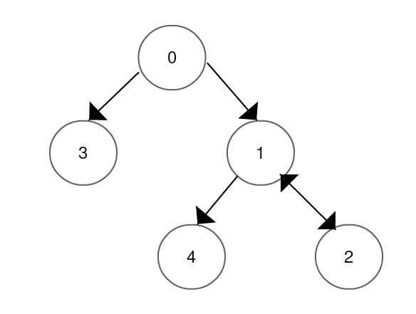
Figure 3: The topology of the leader-follower network of given AUVs.

The leader control law is selected as $u_{0}(t)=K_{0}x_{0}(t)+F_{0}r(t)$, with $K_{0}=1.0e+04[k_{01};k_{02};k_{03};k_{04}]$, $k_{01}=[-0.52,-3.5,-0.65,-8.0]$, $k_{02}=[-0.22,-0.19,0.39,0.48]$, $k_{03}=[-0.04,3.48-0.04,6.47]$, $k_{04}=[-0.25,0.17,0.45,1.19]$, and $F_{0}=1.0e+03[f_{01};f_{02};f_{03};f_{04}]$, $f_{01}=[3.02,-0.14,0.36,6.53]$, $f_{02}=[-0.14,4.02,-1.93,-2.46]$, $f_{03}=[0.36,-1.93,-1.55,3.61]$, $f_{04}=[6.53,-2.46,3.61,-9.55]$, and the desired leader speed $r(t)=\bar{u}_{\text{desired}}(t)$ is defined according to Figure 4. The objective of the team cooperative control is to ensure that all the agents follow the leader output (surge speed) trajectory, while their yaw angle, sway and yaw rate remain bounded. The acceptable errors between the desired trajectory and the actual trajectories are considered to be less than $10\%$ in the steady state. The following scenarios are now considered:

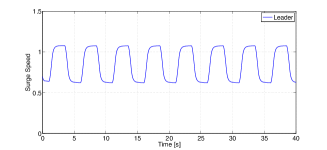
Figure 4: The desired leader surge speed trajectory.

Scenario 1: Faulty team without control reconfiguration: In this scenario, it is assumed that no control reconfiguration is invoked after the occurrence of the faults. The specifics for the mission considered are as follows where the followers state trajectories are depicted in Figure 5.
A) All the agents are healthy and the agent control law is designed according to Theorem 2 and using YALMIP toolbox [Yalmip] for MATLAB. The gains are obtained as $c_{1}=3.926e+06$, $K=1.0e03[k_{1};k_{2};k_{3};k_{4}]$, $k_{1}=[-0.23,0.169,$ $-0.275,-0.039]$, $k_{2}=[-0.26,-0.175,$ $0.278,0.031]$, $k_{3}=[-0.23,0.169,-0.497,-0.039]$, $k_{4}=[-0.026,-0.175,0.278,0.031]$, $C_{2}=1.0e+07\text{diag}\{1.23,1.39,0.39,1.48\}$ and the $H_{\infty}$ upper bound is computed to be $\gamma=0.3687$.
B) At time $t=t_{f}=25\ s$, the agents $1$ and $2$ become faulty. Agent $1$ loses its second actuator i.e. $h_{1fs}^{f}(t)\equiv 0$, $t\geq 25$. Agent $2$ loses $30\%$ of its first actuator and its second actuator gets stuck at $\underline{u}_{2}^{s}=1$, i.e. $h_{2fp}^{f}(t)=0.7h_{2fp}(t)$ and $h_{2fs}^{f}(t)\equiv 1$ for $t\geq 25\ s$.

Figure 5 clearly shows that if a reconfiguration control strategy is not invoked, the agents become unstable and their states grow exponentially unbounded. Therefore, it is necessary to reconfigure the agent’s control law after the occurrence of this fault.

Figure 5: The followers trajectories corresponding to the Scenario 1.

Scenario 2: Control reconfiguration subject to delays in invoking the reconfigured control law: Unlike the previous scenario, in this scenario control reconfiguration laws are invoked to the faulty agents. However, it is assumed that there are delays in the time that the FDI module communicates this information to the faulty agents and the agents reconfigured controls are invoked. The specifics for the execution of the mission are as follows where the followers state trajectories are depicted in Figure 6.
A) All the agents are healthy and the agent control law is similar to the Scenario 1.
B) At time $t=t_{f}=25\ s$, the agents $1$ and $2$ become faulty. The fault scenario that is considered is the same as that of Step B) in Scenario 1.
C) The control laws for both faulty agents are reconfigured according to Theorem 3 at $t=t_{r}=30\ s$ and are set as $K_{11}^{r}=10e03[k_{111};k_{112};k_{113}]$, $k_{111}=[2.627,0.090,-1.895,-4.328]$, $k_{112}=[-2.058,0.09,0.293,3.034]$, $k_{113}=[-0.7549,-0.1799,0.8115,0.4458]$,

$K_{21}^{r}=[k_{211},k_{212},k_{213}]$, $k_{211}=[0.50,0.00,$ $0.50,0.00]$, $k_{212}=[0.50,0.00,0.499,-0.00]$, $k_{213}=[0.00,1.00,-0.00,1.00]$ and $K_{12}^{r}=10e03[k_{121};k_{122};k_{123}]$, $k_{121}=[0.113,0.130,-0.485,-2.89]$, $k_{122}=[0.881,-0.089,-1.263,0.664]$, $k_{123}=[-0.969,0.18,$ $0.697,0.4]$, $K_{22}^{r}=[k_{211},k_{212},k_{213}]$, $k_{211}=[0.7140,0.00,$ $0.7143,0.00]$, $k_{212}=[0.50,0.00,0.499,-0.00]$, $k_{213}=[0.00,1.00,-0.00,1.00]$ and

Figure 6, depicts that by invoking the reconfigured control laws one can now stabilize all the agents. The delay in invoking the control reconfiguration causes a transient period in which the agent states diverge and will not follow the leader (refer to discussion in Subsection III-B, Case V). However, after the transients have died out, the agent reach a consensus with the leader state.

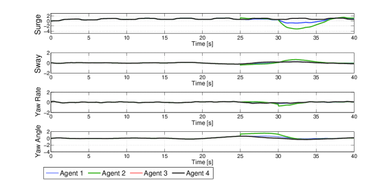
Figure 6: The followers trajectories corresponding to the Scenario 2.

Scenario 3: Control reconfiguration subject to fault estimation uncertainties: In this scenario, we consider a similar fault scenario as in the previous scenarios. However, it is assumed that the estimated fault severities are subject to unreliabilities, errors and uncertainties. Using the inequality (64) the upper bound on uncertainties is obtained as $\bar{\epsilon}_{2max}^{1}=0.146$, implying that the reconfigured control law stabilizes the errors provided that it is designed based on $0.554\leq\hat{\Gamma}_{2}^{1}\leq 0.846$. To investigate how accurate this range is, various levels of uncertainties and mismatches are considered and it is observed that the control gains that are designed for $\hat{\Gamma}_{2}^{1}<0.86$ stabilize the errors whereas for $\hat{\Gamma}_{2}^{1}\geq 0.87$ the state consensus errors become unstable. This indicates that the bound provided by the inequality (64) provides an acceptable approximation to the maximum allowable fault severities estimation errors and uncertainties. The agents state simulation responses correspond to $\hat{\Gamma}_{2}^{1}=0.6$ and $\hat{\underline{u}}_{i}^{s}=0.9$, and are depicted in Figure 7.

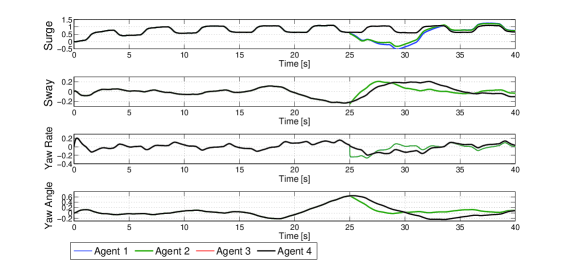
Figure 7: The followers trajectories corresponding to the Scenario 3.

Figure 7 shows that by invoking the reconfigured control law, the agent states will no longer diverge and the recovery control strategy stabilizes the agent states. In fact, in this scenario the agents do follow the changes in the leader speed trajectory, although the error between the faulty agent speed trajectory and the leader speed trajectory will not vanish but converges asymptotically to a small constant value.

Scenario 4: Control reconfiguration subject to uncertainties in the fault isolation: In this scenario, the effects of uncertainties in the fault isolation decision made by the FDI module are studied. It is assumed that the FDI module of agents $1$ and $2$ are subject to fault isolation uncertainties. Two cases are considered as follows:
Scenario 4.1:
A) Similar to Step A) in the Scenario 1.
B) At time $t=20$s the FDI module launches a false fault alarm for the agent $2$, that the second actuator gets stuck at $\underline{u}_{2}^{s}=1$ and its first actuator loses $30\%$ of its efficiency. Then, a reconfigured control is invoked to this agent.
Scenario 4.2:
A) Similar to Step A) in the Scenario 1.
B) At time $t=20$ s agent 2 becomes faulty and a fault scenario similar to Step B) in the Scenario $1$ occurs. However, the FDI module does not detect and isolate this fault in the agent $2$ and instead the FDI module wrongly initiates a fault alarm and a reconfigured control that is applied to the agent $1$.

V Conclusions

In this work, cooperative and distributed reconfigurable control law strategies are developed and designed to control and reconfigure faulty agents from three types of actuator faults, namely loss of effectiveness, outage, and stuck faults that guarantee boundedness of the state consensus errors for a network of multi-agent systems. It is shown that the proposed control strategies can ensure an $H_{\infty}$ performance bound attenuation for the team agents when they are subjected to environmental disturbances and actuator faults. Our proposed reconfigured control laws ensure that the output of the faulty agent matches that of the healthy agent in absence of disturbances. Moreover, the control laws also guarantee that the state consensus errors either remain bounded. Furthermore, in presence of environmental disturbances the $H_{\infty}$ disturbance attenuation bound is ensured to be minimized. The effectiveness of our proposed cooperative control and reconfigurable approaches are evaluated by applying them to a network of five autonomous underwater vehicles. Extensive simulation case studies are also considered to demonstrate the capabilities and advantages of our proposed strategies subject to FDI module uncertainties, erroneous decisions, and imperfections.

References

[1]
S. M. Azizi and K. Khorasani.
Cooperative actuator fault accommodation in formation flight of
unmanned vehicles using relative measurements.
International Journal of Control, 84(5):876–894, 2011.
[2]
A. Bacciotti and F. Ceragioli.
Stability and stabilization of discontinuous systems and nonsmooth
lyapunov functions.
Control, Optimization and Calculus of Variations, 4, 1999.
[3]
G. Basile and G. Marro.
Controlled and Conditioned Invariants in Linear System Theory.
Prentice Hall, Englewood Cliffs, NJ, 1992.
[4]
L. Breger and J. How.
Safe trajectories for autonomous rendezvous of spacecraft.
Journal of Guidance, Control, and Dynamics, 31(5):1478–1489,
2008.
[5]
S. Chen, D. Ho, L. Li, and M. Liu.
Fault-tolerant consensus of multi-agent system with distributed
adaptive protocol.
IEEE Transactions on Cybernetics, 2015.
[6]
S. Croomes.
Overview of the DART mishap investigation results.
NASA Report, pages 1–10, 2006.
[7]
T. Fossen.
Guidance and Control of Ocean Vehicles.
Wiley, 1994.
[8]
T. Fossen.
Marine control systems: Guidance, navigation and control of
ships, rigs and underwater vehicles.
Marine Cybernetics Trondheim, 2002.
[9]
Z. Gallehdari, N. Meskin, and K. Khorasani.
Cost performance based control reconfiguration in multi-agent
systems.
In 2014 American Control Conference, pages 509–516, 2014.
[10]
Z. Gallehdari, N. Meskin, and K. Khorasani.
Robust cooperative control reconfiguration/recovery in multi-agent
systems.
In 2014 European Control Conference (ECC), pages 1554–1561,
2014.
[11]
Z. Gallehdari, N. Meskin, and K. Khorasani.
An cooperative control fault recovery of multi-agent
systems.
http://arxiv.org/abs/1508.07076, 2015.
[12]
M. Jakuba.
Modeling and control of an autonomous underwater vehicle with
combined foil/thruster actuators.
Master’s thesis, Massachusetts Institute of Technology and Woods Hole
Oceanographic Institution, 2003.
[13]
L. Junquan and K. Kumar.
Decentralized fault-tolerant control for satellite attitude
synchronization.
IEEE Transactions on Fuzzy Systems, 20(3):572–586, 2012.
[14]
M. J. Khosrowjerdi, R. Nikoukhah, and N. Safari-Shad.
A mixed H2/H∞ approach to simultaneous fault detection
and control.
Automatica, 40(2):261 – 267, 2004.
[15]
Z. Li, X. Liu, W. Ren, and L. Xie.
Distributed tracking control for linear multi-agent systems with a
leader of bounded unknown input.
IEEE Transactions on Automatic Control, 58(2):518–523, 2013.
[16]
L. Liu, Y. Shen, E. H. Dowell, and C. Zhu.
A general fault tolerant control and management for a linear system
with actuator faults.
Automatica, 48(8):1676 – 1682, 2012.
[17]
J. Lunze and T. Steffen.
Control reconfiguration after actuator failures using disturbance
decoupling methods.
IEEE Transactions on Automatic Control, 51(10):1590–1601,
2006.
[18]
G. Marro.
Geometric approach toolbox.
http://www3.deis.unibo.it/Staff/FullProf/GiovanniMarro/geometric.htm,
2010.
[19]
A.R. Mehrabian, S. Tafazoli, and K. Khorasani.
Reconfigurable control of networked nonlinear Euler-Lagrange
systems subject to fault diagnostic imperfections.
In 50th IEEE Conference on Decision and Control and European
Control Conference (CDC-ECC), pages 6380–6387, 2011.
[20]
A.R. Mehrabian, S. Tafazoli, and K. Khorasani.
State synchronization of networked Euler-Lagrange systems with
switching communication topologies subject to actuator faults.
In 18th IFAC World Congress Milano (Italy), 2011.
[21]
K. H. Movric and F. L. Lewis.
Cooperative optimal control for multi-agent systems on directed graph
topologies.
IEEE Transactions on Automatic Control, 59(3):769–774, 2014.
[22]
Xavier O.
FDI(R) for satellites: How to deal with high availability
and robustness in the space domain?
International Journal of Applied Mathematics and Computer
Science, 22(1):99 107, 2012.
[23]
E. Semsar-Kazerooni and K. Khorasani.
Multi-agent team cooperation: A game theory approach.
Automatica, 45(10):2205–2213, 2009.
[24]
D. Shevitz and B. Paden.
Lyapunov stability theory of nonsmooth systems.
IEEE Transactions on Automatic Control, 39(9):1910–1914, 1994.
[25]
M. M. Tousi and K. Khorasani.
Optimal hybrid fault recovery in a team of unmanned aerial vehicles.
Automatica, 48(2):410 – 418, 2012.
[26]
X. Wang and G. H. Yang.
Cooperative adaptive fault-tolerant tracking control for a class of
multi-agent systems with actuator failures and mismatched parameter
uncertainties.
IET Control Theory Applications, 9(8):1274–1284, 2015.
[27]
Y. Wang, Y. Song, and F.L. Lewis.
Robust adaptive fault-tolerant control of multiagent systems with
uncertain nonidentical dynamics and undetectable actuation failures.
IEEE Transactions on Industrial Electronics, 62(6):3978–3988,
2015.
[28]
R. Wei.
Consensus tracking under directed interaction topologies: Algorithms
and experiments.
IEEE Transactions on Control Systems Technology,
18(1):230–237, 2010.
[29]
B. Xiao, Q. Hu, and P. Shi.
Attitude stabilization of spacecrafts under actuator saturation and
partial loss of control effectiveness.
IEEE Transactions on Control Systems Technology,
21(6):2251–2263, 2013.
[30]
G. H. Yang and D. Ye.
Adaptive actuator failure compensation control of uncertain nonlinear
systems with guaranteed transient performance.
Automatica, 46(12):2082 – 2091, 2010.
[31]
R. K. Yedavalli.
Robust Control of Uncertain Dynamic Systems:A Linear State Space
Approach.
Springer New York, 2014.
[32]
L. Zhao and Y. Jia.
Neural network-based adaptive consensus tracking control for
multi-agent systems under actuator faults.
International Journal of Systems Science, 21(6):2251–2263,
2014.
[33]
B. Zhou, W. Wang, and H. Ye.
Cooperative control for consensus of multi-agent systems with
actuator faults.
Computers Electrical Engineering, 40(7):2154 – 2166,
2014.