Modelling galaxy clustering: halo occupation distribution versus subhalo matching

Abstract

We model the luminosity-dependent projected and redshift-space two-point correlation functions (2PCFs) of the Sloan Digital Sky Survey (SDSS) Data Relese 7 Main galaxy sample, using the halo occupation distribution (HOD) model and the subhalo abundance matching (SHAM) model and its extension. All the models are built on the same high-resolution $N$-body simulations. We find that the HOD model generally provides the best performance in reproducing the clustering measurements in both projected and redshift spaces. The SHAM model with the same halo-galaxy relation for central and satellite galaxies (or distinct haloes and subhaloes), when including scatters, has a best-fitting $\chi^{2}/\rm{dof}$ around $2$–$3$. We therefore extend the SHAM model to the subhalo clustering and abundance matching (SCAM) by allowing the central and satellite galaxies to have different galaxy–halo relations. We infer the corresponding halo/subhalo parameters by jointly fitting the galaxy 2PCFs and abundances and consider subhaloes selected based on three properties, the mass $M_{\rm acc}$ at the time of accretion, the maximum circular velocity $V_{\rm acc}$ at the time of accretion, and the peak maximum circular velocity $V_{\rm peak}$ over the history of the subhaloes. The three subhalo models work well for luminous galaxy samples (with luminosity above $L_{*}$). For low-luminosity samples, the $V_{\rm acc}$ model stands out in reproducing the data, with the $V_{\rm peak}$ model slightly worse, while the $M_{\rm acc}$ model fails to fit the data. We discuss the implications of the modelling results.

1 Introduction

The connection between the observed galaxy distribution and the underlying dark matter is a fundamental question in modern cosmology. It can help us understand the dark matter component of the energy density distribution from the observed baryon components. The contemporary galaxy formation models assume that galaxies form and evolve within the dark matter haloes (White & Rees, 1978). Therefore, we can use the dark matter haloes to build the connection between the luminous and dark sides of the universe.

There are multiple ways of linking galaxies to the dark matter haloes. The most straightforward method is to employ the hydrodynamic simulations to take into account the complicated physics involved in the galaxy formation and evolution (see the latest such simulations in e.g. Vogelsberger et al., 2014a; Schaye et al., 2015), as well as the semi-analytic models that are built on the halo merger trees from $N$-body dark matter simulations (e.g. Bower et al., 2006; Croton et al., 2006; Somerville et al., 2008; Guo et al., 2011). But the poorly understood galaxy formation physical processes related to baryons make such methods model dependent and difficult to satisfactorily reproduce the observations in the current data accuracy. Other statistical methods are then developed to evade the necessity of including the galaxy formation physics and to make use of the population of dark matter haloes whose formation is dominated by gravity and well understood. Such methods aim at empirically establishing the connection between galaxies and dark matter haloes from statistical distributions of galaxies like galaxy clustering, and then the galaxy-halo connection is used to constrain galaxy formation and evolution. The most popular models are the halo occupation distribution (HOD; Jing et al., 1998; Peacock & Smith, 2000; Berlind & Weinberg, 2002; Zheng et al., 2005; Zheng et al., 2009; Leauthaud et al., 2012; Guo et al., 2014; Skibba et al., 2015; Zu & Mandelbaum, 2015), the closely related conditional luminosity function (CLF; Yang et al., 2003; Yang et al., 2004), and the subhalo abundance matching (SHAM; Kravtsov et al., 2004; Conroy et al., 2006; Vale & Ostriker, 2006; Wang et al., 2007; Behroozi et al., 2010; Guo et al., 2010; Moster et al., 2010; Nuza et al., 2013; Rodríguez-Puebla et al., 2013; Sawala et al., 2015; Yamamoto et al., 2015). All of these methods are based on the halo framework, by assuming that all galaxies reside in the haloes. In this paper we focus on the detailed and quantitative model comparisons between the HOD and SHAM methods.

The HOD description includes the probability $P(N|M)$ of finding $N$ galaxies of certain properties in a dark matter halo of virial mass $M$, and the spatial and velocity distribution of those galaxies inside haloes. Analytical methods have been developed within the HOD (or CLF) framework to compute galaxy clustering statistics (e.g. Zheng, 2004; Tinker et al., 2005; van den Bosch et al., 2013). By using dark matter haloes identified in high-resolution $N$-body simulations, the HOD model can be made accurate enough to interpret the observed high-precision galaxy clustering measurements from large galaxy surveys (Zheng & Guo, 2016), which overcomes the difficulty of modelling the effects of halo exclusion, nonlinear growth, and scale-dependent halo bias in the analytical HOD models (e.g. Zheng, 2004; Tinker et al., 2005). Based on galaxy formation models, galaxies in the HOD model are further categorized into central and satellite galaxies according to their spatial distribution within the haloes. In many applications, central galaxies are usually put at halo centres and assumed to have the velocities of the haloes, while satellite galaxies are assumed to follow the spatial and velocity distributions of the dark matter in the haloes. However, the HOD description itself allows the freedom of varying the above assumptions, by introducing spatial bias and velocity bias. For example, the recent modelling of small-scale redshift-space clustering measurements using both the Sloan Digital Sky Survey (SDSS) Main galaxy sample (Guo et al., 2015c) and SDSS-III Baryon Oscillation Spectroscopic Survey (Guo et al., 2015a) shows that central galaxies have velocity offsets with respect to the halo bulk velocities and the velocity distribution of satellite galaxies generally differs from that of the dark matter. By including such velocity bias factors, the HOD model is able to reproduce the observed galaxy two-point correlation functions (2PCFs) in both projected and redshift spaces remarkably well and to interpret successfully higher-order statistics, like the three-point correlation functions (Guo et al., 2015b).

The development of the high-resolution $N$-body simulations enables the identification of the substructures within the dark matter haloes, i.e. the subhaloes, which were distinct haloes before they fell into the current host haloes (see e.g. Klypin et al., 2016; Pujol et al., 2014). As in the literature, we refer to virialized haloes that are not subhaloes of another halo as distinct haloes. The subhaloes are believed to be the natural local environments for the satellite galaxies in the host haloes. Due to their trackable merger histories, the subhaloes provide a powerful way to study the galaxy evolution once the connection between satellite galaxies and subhaloes is built. The basic idea of the SHAM method is to assume a monotonic relation between certain galaxy property and certain halo (including subhalo) property. For example, the one-to-one correspondence between the galaxies and the dark matter haloes (and subhaloes) can be made by ranking the galaxies in order of their luminosity and populating the more massive haloes (and subhaloes) with more luminous galaxies, i.e. the number density of galaxies above a luminosity threshold is matched to that of haloes above a mass threshold, establishing a link between galaxy luminosity and halo mass. In this way, the galaxies relating to the host haloes are naturally central galaxies while those in the subhaloes are satellite galaxies. In practice, the SHAM method always includes a scatter in the galaxy-halo/subhalo relation, which has its physical origin.

Accurately identifying and defining the subhaloes in the simulations should take into account the effects of both the simulation resolution and baryon physics (Weinberg et al., 2008). While the resolution effect is less severe with the emergence of more and more high-resolution simulations, the baryon physics can still give rise to an important systematic effect for the SHAM method. Compared to the stellar components of satellite galaxies that are more gravitationally bound, the dark matter in subhaloes suffers more from tidal heating and stripping. Galaxy properties are therefore more closely connected to subhalo properties that are less affected by the tidal effects. The original SHAM method is improved by relating the satellite galaxy properties to the maximum circular velocity or the mass of subhaloes at the epoch of accretion (see e.g. Conroy et al., 2006; Vale & Ostriker, 2006) or over the entire merger history (see e.g. Moster et al., 2010; Reddick et al., 2013). Such improvement is shown to reproduce better the observed galaxy clustering measurements. However, some effects are yet to be taken into account in the SHAM model. For example, some subhaloes can be tidally destructed while the corresponding satellite galaxies (stellar component) can still survive (the so-called orphan galaxies; Wang et al., 2006; Moster et al., 2010), and the usual SHAM model based on $N$-body simulations would miss such a population.

The different halo and subhalo models have been studied extensively in the previous literature (see e.g. Yang et al., 2012). Yang et al. (2009) used CLF method to explore the consequence of the stellar mass evolution of the satellite galaxies assuming the same stellar-halo mass relation (SHMR) for host haloes at present day and subhaloes at the time of accretion. They used the galaxy group catalogues (Yang et al., 2005) constructed from SDSS DR4 to predict the stellar mass function of the satellite galaxies and emphasize the importance of including intracluster stars in the galaxy evolution. Neistein et al. (2011a) studied the SHMR for central and satellite galaxies in the SHAM using a set of semi-analytical models (SAMs). They found that adopting the same SHMR for central and satellite galaxies cannot reproduce the clustering measurements in SAMs. Neistein et al. (2011b) further extended the SHAM models by allowing the stellar mass of the satellite galaxies to also depend on the host halo mass and concluded that the SHMR is not well constrained from the clustering measurements alone. Rodríguez-Puebla et al. (2012) also found that different SHMRs for central and satellite galaxies are favoured by the observation by using the central and satellite stellar mass functions from the galaxy group catalogues. The SHAM technique is also examined in the smoothed particle hydrodynamics simulations by Simha et al. (2012), and it is found to overpopulate massive haloes because of severe stellar mass loss of some satellite galaxies. Reddick et al. (2013) compared the connection between different halo properties and the galaxy stellar mass in the SHAM models. The scatter between galaxy stellar mass and halo property is constrained by the galaxy clustering measurements and the conditional stellar mass functions. They found that the model with the halo peak circular velocity provides the best agreement with the data.

The galaxy projected 2PCFs have been extensively used previously in constraining the models. However, the redshift-space clustering measurements have additional information about the galaxy velocity field and therefore can help distinguish different models. In this paper, we compare quantitatively the HOD and (extended) SHAM methods in modelling both the projected and redshift-space clustering of the volume-limited luminosity-threshold galaxy samples in the SDSS Data Release 7 (DR7). The galaxy-halo connections for the central and satellite galaxies are allowed to be different in the extended SHAM models. Unlike Rodríguez-Puebla et al. (2012), who apply SHAM separately to central and satellite stellar mass functions based on a group catalogue, we constrain all parameters of the extended SHAM models using the galaxy clustering measurements and the galaxy sample number densities. In Section 2, we describe the measurements of our galaxy samples and the modelling method. The subhalo distributions in the high-resolution simulations are investigated in Section 3. We present the results of modelling the projected and redshift-space clustering measurements in Sections 4 and 5, respectively. Finally, we summarize our results and discuss the possible applications in Section 6. Throughout the paper, we assume a spatially flat $\Lambda$ cold dark matter cosmology, with $\Omega_{m}=0.307$, $h=0.678$, and $\sigma_{8}=0.823$, consistent with the constraints from Planck (Planck Collaboration, 2014). The halo mass used in this paper is calculated based on the given spherical overdensities of a viral structure (Bryan & Norman, 1998).

2 Measurements and Models

In this paper, we use the galaxies in the New York University Value-Added Galaxy Catalog (NYU-VAGC; Blanton et al., 2005) for the SDSS DR7 Main galaxy sample (Abazajian et al., 2009). We further construct eight volume-limited luminosity threshold samples, with absolute r-band Petrosian magnitude $M_{r}$ varying from $-18$ to $-21.5$ with step size of $0.5$. We refer the readers to Guo et al. (2015c, hereafter G15) for more details.

The projected 2PCF $w_{p}(r_{p})$ and redshift-space 2PCF monopole ($\xi_{0}(s)$), quadrupole ($\xi_{2}(s)$) and hexadecapole ($\xi_{4}(s)$) moments are measured for each sample, where $r_{p}$ and $s$ are the transverse and redshift-space separations of galaxy pairs, respectively. The galaxy 2PCF measurements range from small scales of $0.1\,h^{-1}{\rm{Mpc}}$ to intermediate scales of $25\,h^{-1}{\rm{Mpc}}$. The projected 2PCF $w_{p}(r_{p})$ is measured by integrating the redshift-space 3D 2PCF to a maximum light-of-sight pair separation of $40\,h^{-1}{\rm{Mpc}}$ (also adopted in all the models). The covariance matrix for each sample is estimated from jackknife resampling method (Zehavi et al., 2011; Guo et al., 2013).

We follow the simulation-based model method laid out in Zheng & Guo (2016) to interpret the galaxy 2PCF measurements within the HOD and SHAM frameworks. It has been used in G15 and Guo et al. (2015a). With haloes identified in a high-resolution N-body simulation, this method tabulates all the necessary halo components in calculating galaxy 2PCFs, including one-halo pair distributions and two-halo 2PCFs from pairs composed of different combinations of central and satellite galaxies. With such tables and a specified description/parametrization of galaxy-halo relation (e.g. within the HOD and SHAM frameworks), galaxy 2PCFs are simply obtained by summing over different, pre-calculated table elements, weighted by the corresponding galaxy occupation statistics. With a given set of HOD (and SHAM) parameters, this method is equivalent to, but more efficient than, directly assigning galaxies to haloes (and subhaloes) in the simulation and measuring the corresponding model 2PCFs. Compared to analytical models, it ensures high accuracy by using the halo information directly from the simulations and by calculating 2PCFs with exactly the same binning scheme as in the data. Finally, this method provides an efficient way to explore the parameter space for different models, which serves well our purpose in this paper.

We use the MultiDark simulation of Planck cosmology (MDPL; Klypin et al. 2016), with the cosmological parameters of $\Omega_{m}=0.307$, $\Omega_{b}=0.048$, $h=0.678$, $n_{s}=0.96$, and $\sigma_{8}=0.823$. The simulation has a volume of 1 $h^{-3}$ Gpc³ (comoving) and the mass resolution is as low as $1.51\times 10^{9}\,h^{-1}{\rm M_{\sun}}$. The simulation output at $z=0$ is adopted to model all our luminosity threshold galaxy samples. To see how simulation resolution affects the subhalo population, we also investigate a smaller simulation that has the same cosmological parameters as MDPL, but with a volume of $0.4^{3}\,h^{-3}$ Gpc³, which is referred to as SMDPL (Klypin et al., 2016). This simulation was run with the same number of particles ($3840^{3}$) as in MDPL, so its mass resolution is $9.6\times 10^{7}\,h^{-1}{\rm M_{\sun}}$, about 15.6 times finer than MDPL.

In both MDPL and SMDPL, the dark matter haloes and subhaloes are identified with the Rockstar phase-space halo finder (Behroozi et al., 2013), where the spherical haloes are found from the density peaks in the phase space. The Rockstar code is efficient and accurate to find the bound (sub)structures in the simulations (Onions et al., 2012; Knebe et al., 2013). Note that different from G15, the unbound particles are removed from our halo (and subhalo) catalogue. The halo (subhalo) velocities are defined as the average particle velocity within the innermost 10% of the halo (subhalo) radius, which is different from the definition of centre-of-mass velocity (i.e. bulk velocity) of haloes in G15. The different halo velocity definitions will affect the inferred galaxy velocity bias parameters. This change of halo definition is to match those in the publicly available Rockstar halo and subhalo catalogues. However, since we use the same halo catalogues for the HOD and SHAM models, the comparison in this paper is not affected by the definitions of haloes and halo properties. We consider three sets of models to connect galaxies to the dark matter haloes in the following sections. To avoid confusion, the host haloes and distinct haloes mentioned hereafter refer to the haloes that are not subhaloes of any other dark matter haloes.

2.1 The HOD Model

For a sample of galaxies above a given luminosity threshold, the HOD model includes five parameters for describing the average number $N$ of galaxies in distinct haloes of mass $M_{\rm h}$ (Zheng, Coil & Zehavi, 2007)

$$\langle N(M_{\rm h})\rangle = \langle N_{\rm cen}(M_{\rm h})\rangle+\langle N_{\rm sat}(M_{\rm h})\rangle,$$ (1)

$$\langle N_{\rm cen}(M_{\rm h})\rangle = \frac{1}{2}\left[1+{\rm erf}\left(\frac{\log M_{\rm h}-\log M_{\rm min}}{\sigma_{\log M_{\rm h}}}\right)\right],$$ (2)

$$\langle N_{\rm sat}(M_{\rm h})\rangle = \langle N_{\rm cen}(M_{\rm h})\rangle\left(\frac{M_{\rm h}-M_{0}}{M_{1}^{\prime}}\right)^{\alpha},$$ (3)

where the two central galaxy parameters $M_{\rm min}$ and $\sigma_{\log M_{\rm h}}$ describe the characteristic minimum mass of haloes that host the sample of galaxies ($\langle N_{\rm cen}(M_{\rm min})\rangle=0.5$) and the characteristic width of the transition mass range for haloes hosting zero to one galaxy. The three parameters for the satellite galaxies are the cutoff mass scale $M_{0}$, the normalization mass scale $M_{1}^{\prime}$ and the power-law slope $\alpha$ at the high-mass end. In this paper, we fix $\alpha\equiv 1$ in order to match the slope of the subhalo occupation function in massive haloes and to reduce the degrees of freedom (dof) to match that in the SHAM model (see below). In the following sections, we also compare two useful derived parameters, the characteristic mass $M_{1}$ of haloes hosting on average one satellite galaxy and the inferred satellite fraction $f_{\rm sat}$ (defined as the fraction of the satellite galaxies in the sample).

We note that to compute the mean number of intra-halo central-satellite pairs in the model, the occupation numbers of central and satellite galaxies are assumed to be independent of each other. That is, we have $\langle N_{\rm cen}N_{\rm sat}\rangle=\langle N_{\rm cen}\rangle\langle N_{\rm sat}\rangle$. Changing the assumption of the dependence between the central and satellite occupations only has minimal effects on the HOD parameters, as discussed in Fig. 10 of Guo et al. (2015a). Compared to the case of having satellites only in haloes with central galaxies for a given galaxy sample, we now can populate satellites in some low mass haloes without central galaxies. As a consequence, the best-fitting $\alpha$ will decrease and the central galaxy velocity bias will slightly shift to lower values, while other HOD parameters only change by about 0.1%.

In our fiducial model, the central galaxies are assigned the positions and velocities of the distinct haloes, while the random dark matter particles in the haloes are selected to represent the satellite galaxies. As in G15, we introduce an additional central galaxy velocity bias parameter $\alpha_{c}$ in the HOD model to allow the central galaxy velocity to differ from that of the halo velocity, with a velocity dispersion equal to $\alpha_{c}$ times the dark matter particle velocity dispersion $\sigma_{v}$ in the haloes. We also include the satellite velocity bias parameter $\alpha_{s}$. The relative velocity of a satellite galaxy to the halo centre is scaled by the satellite velocity bias $\alpha_{s}$ to take into account the possible velocity differences between the dark matter particles and the satellite galaxies. In the frame of a single halo, the satellite galaxy velocity bias is the same as the ratio between the velocity dispersions of the satellite galaxies ($\sigma_{\rm sat}$) and the dark matter particles within the haloes, i.e. $\alpha_{s}=\sigma_{\rm sat}/\sigma_{v}$. We refer the readers to G15 for more details. In total, we have six free parameters in the HOD model, four for the mean occupation function ($M_{\rm min}$, $\sigma_{\log M_{h}}$, $M_{0}$, and $M_{1}^{\prime}$) and two for the velocity bias ($\alpha_{c}$ and $\alpha_{s}$).

We apply a Markov Chain Monte Carlo (MCMC) method to explore the probability distribution of the model parameters. The likelihood surface is determined by $\chi^{2}$, contributed by the projected 2PCF $w_{p}$, the redshift-space multipoles $\xi_{0}$, $\xi_{2}$ and $\xi_{4}$, and the observed galaxy number density $n_{g}$,

$$\chi^{2}=\mn@boldsymbol{(\xi-\xi^{*})^{T}C^{-1}(\xi-\xi^{*})}+\frac{(n_{g}-n_{g}^{*})^{2}}{\sigma_{n_{g}}^{2}},$$ (4)

where $\mn@boldsymbol{C}$ is the full error covariance matrix and the data vector $\mn@boldsymbol{\xi}=[\mn@boldsymbol{w_{p}},\mn@boldsymbol{\xi_{0}},\mn@boldsymbol{\xi_{2}},\mn@boldsymbol{\xi_{4}}]$. The quantity with (without) a superscript ‘$*$’ is the one from the measurement (model). To take into account the finite volume of the simulations our model is based on, we also apply a volume correction of $1+V_{\rm obs}/V_{\rm sim}$ to the covariance matrix (Zheng & Guo, 2016), where $V_{\rm obs}$ and $V_{\rm sim}$ are the volumes for the observed galaxy sample and the simulation, respectively. For each sample and each model, we perform MCMC runs with length of two million to explore the parameter space and to choose the set of best-fitting parameters. For the chain, at each step of the random walk, a set of trial HOD parameters are generated. Covariances among parameters are taken into account when proposing the trial move in order to improve the efficiency of the chain. The probability of keeping the trial HOD parameters depends on the difference $\Delta\chi^{2}=\chi^{2}_{\rm new}-\chi^{2}_{\rm old}$ between the old and new (trial) sets of parameters, i.e. 1 for $\Delta\chi^{2}\leq 0$ and $\exp(-\Delta\chi^{2}/2)$ for $\Delta\chi^{2}>0$.

2.2 The SHAM Models

The simplest SHAM model usually assumes a monotonic relation between the galaxy luminosity (or stellar mass) and a given halo property (e.g. halo mass), by assigning more luminous galaxies to more massive haloes. The galaxy luminosity function is then preserved by matching the number density of the galaxy sample to that of the haloes (see e.g. Conroy et al., 2006). Since such an assignment is only based on the halo property (e.g. halo mass), the distinct halo and subhalo in the simulations are not distinguished between each other. The relation between the galaxies and the haloes (including both distinct haloes and subhaloes) is completely determined by the number density distribution (e.g. luminosity function) of the galaxy sample. Thus, there is no free parameter in such models. A more flexible SHAM model is typically introduced to allow a scatter between e.g. the galaxy luminosity and the halo mass. Such a scatter is necessary especially when modelling the clustering of the luminous galaxies (see e.g. Reddick et al., 2013).

There are a few popular SHAM models that connect the galaxy luminosity to the different halo properties. In this paper, we only consider the following three SHAM models using different halo properties.

(1) $M_{\rm acc}$. For a distinct halo, it is the current halo mass, while for a subhalo, it is the mass at the last epoch when the subhalo was a distinct halo (before accreted to another halo).

(2) $V_{\rm acc}$. For a distinct halo, it is the current maximum circular velocity, while for a subhalo, it is the maximum circular velocity at the last epoch of being a distinct halo (before accreted to another halo).

(3) $V_{\rm peak}$. For both distinct haloes and subhaloes, it is the peak circular velocity over the entire merger history.

The properties $M_{\rm acc}$ and $V_{\rm acc}$ are commonly used in the SHAM models because they are closely related to the halo merger history, while recent results suggest that choosing $V_{\rm peak}$ in the model leads to better agreement with the data (e.g. Moster et al., 2010). The $V_{\rm peak}$ of a distinct halo or subhalo is usually significantly larger than $V_{\rm acc}$, because the peak circular velocity is generally achieved earlier in time than the accretion. The tidal heating and stripping will later reduce the circular velocity of a subhalo even before the accretion (see e.g. Fig. 1 of Chaves-Montero et al., 2015). Reddick et al. (2013) compared different SHAM models and found that $V_{\rm peak}$ is more closely related to the galaxy stellar mass, while $M_{\rm peak}$ (the maximum mass that a halo or subhalo has ever had in its merger history) is generally not successful in reproducing the clustering measurements. So we do not consider the $M_{\rm peak}$ case in our SHAM models. We will investigate these three models in the following sections.

In implementing the SHAM models we allow a scatter between the galaxy property (here luminosity) and the adopted halo property. To facilitate the comparison with the HOD model, the scatter is parametrized in a way of using the functional form of Eq. 2 to assign galaxies to haloes. As an example of choosing $M_{\rm acc}$ as the halo property, the probability of a distinct halo or subhalo having a galaxy in a given luminosity-threshold sample is

$$P(M_{\rm acc})=\frac{1}{2}\left[1+{\rm erf}\left(\frac{\log M_{\rm acc}-\log M_{\rm min,acc}}{\sigma_{\log M_{\rm acc}}}\right)\right]$$ (5)

The scatter between galaxy property and halo property is encoded in the parameter $\sigma_{\log M_{\rm acc}}$ (Zheng et al., 2007), which is the only free parameter in Eq. 5. The characteristic mass scale $M_{\rm min,acc}$ can then be determined by matching the sample number density. For other two halo properties, we only need to replace the mass in Eq. 5 to the corresponding terms for $V_{\rm acc}$ and $V_{\rm peak}$. Note that the SHAM model we use here is more flexible than the commonly adopted one. The usual SHAM model assumes one scatter parameter and performs the abundance matching for galaxies in the full range of observed luminosity. Here we model a series of luminosity-threshold samples, and each has its own scatter parameter. We are effectively allowing the scatter between the galaxy luminosity and the halo property to vary with the halo property.

In the SHAM model we use, a further improvement is related to the determination of the scatter parameter. We do not simply assign a scatter parameter for a given luminosity-threshold sample. The final $\sigma_{\log M_{\rm acc}}$ used in each luminosity-threshold sample is determined from the model with the best-fitting $\chi^{2}$ to the galaxy projected 2PCFs. We emphasize that even though the scatter parameter we introduce here is formally expressed in terms of the halo property (mass or circular velocity), it is originally derived from the scatter in the (lognormal) galaxy luminosity distribution at a fixed halo mass or circular velocity (see Eq. 4 in Zheng et al., 2007). The meaning of $\sigma_{\log M_{\rm acc}}$ is not the scatter on the halo mass at a fixed galaxy luminosity, but rather the width of the cutoff profile. We can conveniently convert $\sigma_{\log M_{\rm acc}}$ to the scatter on the galaxy luminosity $\sigma_{\log L}$ at fixed halo mass using the local slope of the $L$–$M_{\rm acc}$ relation at the threshold luminosity, as will be shown in the following sections.

For central galaxy occupation distribution in the $M_{\rm acc}$ model, we can directly compare $M_{\rm min,acc}$ to $M_{\rm min}$ in the HOD model, because they both refer to the typical cutoff mass of the distinct haloes that host the galaxies in the sample of interest. For satellite galaxies in subhaloes of $M_{\rm acc}$ at the time of accretion, with the simulations we can conveniently convert $P(M_{\rm acc})$ in Eq. 5 to the satellite mean occupation function $\langle N_{\rm sat}(M_{\rm h})\rangle$ in host haloes of mass $M_{\rm h}$. From the average occupation number $\langle N_{\rm sub}(M_{\rm acc}|M_{\rm h})\rangle$ of subhaloes with mass $M_{\rm acc}$ in each host halo with mass $M_{\rm h}$, we have

$$\langle N_{\rm sat}(M_{\rm h})\rangle=\sum_{M_{\rm acc}}P(M_{\rm acc})\langle N_{\rm sub}(M_{\rm acc}|M_{\rm h})\rangle.$$ (6)

For the cases of $V_{\rm acc}$ and $V_{\rm peak}$ models, the mean satellite function can be computed similarly by replacing the mass in Eq. 6 to the corresponding velocity variable.

Overall, the SHAM model we use here is more flexible, compared to the traditional one. We allow the scatter to depend on the halo property, and determine it by fitting the projected 2PCF. The number density of the galaxy sample is ensured to be matched by tuning the characteristic halo mass scale $M_{\rm min,acc}$. In what follows, we further extend or generalize the SHAM model to make it even more flexible, with the relevant parameters determined by both the galaxy abundance and the galaxy clustering (in projected and redshift spaces).

2.3 A Subhalo Clustering and Abundance Matching Model

The galaxy luminosity (or halo mass/property) dependent scatter extends the SHAM models. However, as will be shown below, this extension is still not capable of satisfactorily interpreting the observed galaxy 2PCFs. We therefore add further flexibilities to the SHAM model and make it a well parametrized model to fit both the galaxy abundance and clustering, which can be referred to as subhalo clustering and abundance matching (SCAM) model.

For a given luminosity-threshold galaxy sample, we construct the SCAM model by allowing the mass scale $M_{\rm min,acc}$ and scatter parameter $\sigma_{\log M_{\rm acc}}$ in Eq. 5 to be different for the distinct haloes (central galaxies) and subhaloes (satellites). That is, we now have probabilities $P_{\rm cen}(M_{\rm acc})$ and $P_{\rm sat}(M_{\rm acc})$. The extensions for the case of $V_{\rm acc}$ and $V_{\rm peak}$ are similar. Once a halo property is chosen to use, we have four parameters for the central and satellite mean occupation functions. Such separate parametrizations for the central and satellite components in the SCAM model are supported by the recent findings of the differences between the central and satellite galaxies in the SHAM models (Rodríguez-Puebla et al., 2012; Watson & Conroy, 2013).

To model the redshift-space 2PCFs with the SCAM model, the treatment of the central galaxies is the same as in the HOD model and a central galaxy velocity bias parameter $\alpha_{c}$ is introduced. Since the subhaloes are selected to host satellite galaxies, we also apply a satellite galaxy velocity bias by scaling the velocity of a subhalo relative to its host halo with a factor of $\alpha_{s}$. So in total we have six free parameters for the redshift-space modelling with the SCAM model. As with the HOD model, the parameter space is explored with the MCMC method with the likelihood determined by the 2PCFs and the galaxy number density (Eq. 4).

3 Particle and Subhalo Distributions in Simulations

Before we apply the HOD/SHAM/SCAM models to model the clustering measurements, it is important to understand the particle and subhalo distributions in the simulations. As subhaloes are related to satellites in SHAM/SCAM, the HOD model in this paper connects satellites to dark matter particles. Any difference seen in the particle and subhalo distributions will be useful for us to understand the modelling results.

Figure 1: Comparisons of the subhalo distributions between the MDPL and SMDPL simulations. In each panel, solid and dotted curves are from the MDPL and SMDPL simulations, respectively. Panel (a): subhalo mass functions. Panel (b): subhalo spatial distribution profile in the host haloes of $M_{\rm h}{\sim}10^{13}\,h^{-1}{\rm M_{\sun}}$. The red and blue curves are for subhaloes selected using different mass or velocity thresholds. For the $M_{\rm acc}$ model, the red and blue curves are for $M_{\rm acc}>10^{12}$ and $>10^{11.5}\,h^{-1}{\rm M_{\sun}}$, respectively. For the $V_{\rm acc}$ and $V_{\rm peak}$ models, the red and blue curves are for $V_{\rm acc}$ (or $V_{\rm peak}$) larger than $10^{2.3}$ and $10^{2.1}\,{\rm{km\,s^{-1}}}$, respectively. For each model, the profiles are normalized to be the same at the host halo virial radius and the curves are separated for different models for clarity. The black solid lines are the density profiles for the dark matter particles in each case. Panel (c): similar to panel (b), but for the host haloes of $M_{\rm h}{\sim}10^{14}\,h^{-1}{\rm M_{\sun}}$. Panel (d): 3D dark matter velocity dispersion in distinct haloes of different mass $M_{\rm h}$. The shaded area shows the scatter around the velocity dispersion measurements in SMDPL.

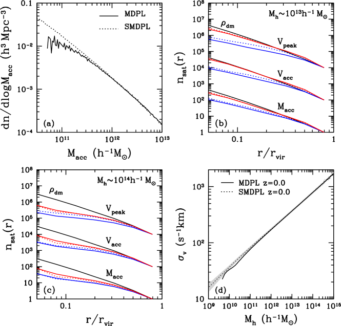
We show in Fig. 1 the detailed comparisons between the subhalo distributions in the MDPL and SMDPL simulations. Panel (a) shows the subhalo mass functions in the two simulations. The simulation resolution does affect the identification of the subhaloes in the two simulations. But for subhaloes of $M_{\rm acc}>2.8\times 10^{11}\,h^{-1}{\rm M_{\sun}}$, the subhaloes in MDPL are about 90% complete, compared to that of the SMDPL. In terms of circular velocities, subhaloes are 90% complete in MDPL for $V_{\rm acc}>176\,{\rm{km\,s^{-1}}}$ and $V_{\rm peak}>184\,{\rm{km\,s^{-1}}}$, respectively.

Figure 2: Best-fitting models for the projected 2PCF $w_{p}(r_{p})$ using the different SHAM models with scatters. The measurements for volume-limited samples in SDSS DR7 Main galaxies are shown as the circles with error bars. The different SHAM models are shown as the different colour lines as labelled. The ratios between the SHAM models and the measurements are shown in the bottom part of each panel, with the error bars from the measurements.

As will be shown in the following sections, many faint satellite galaxies in the SHAM/SCAM model are predicted to reside in subhaloes of mass $M_{\rm acc}$ around $10^{11}\,h^{-1}{\rm M_{\sun}}$. The corresponding subhaloes identified in MDPL simulation suffer from the resolution effect, so for the SHAM/SCAM method we will model the faint galaxy samples of $M_{r}<-18$, $-18.5$, $-19$, and $-19.5$ using the SMDPL simulation instead and model the more luminous samples using the MDPL simulation. The volume $V_{\rm sim}$ of the SMDPL is much larger than the survey volume $V_{\rm obs}$ of these faint samples (G15), so the volume correction (the $1+V_{\rm obs}/V_{\rm sim}$ factor) to the covariance matrix (Zheng & Guo, 2016) is not significant. For the HOD model, since we are randomly selecting the dark matter particles to represent the satellite galaxies, the resolution of the MDPL simulation is high enough to model all the luminosity threshold samples. So we do not use the SMDPL for the HOD models. We have verified that using SMDPL for modelling the faint galaxy samples with the HOD method produces the same results as using the MDPL simulation. This is consistent with the fact that the mass functions for the distinct haloes in MDPL and SMDPL agree down to haloes of about $5\times 10^{10}\,h^{-1}{\rm M_{\sun}}$ (Rodriguez-Puebla et al., 2016).

Panels (b) and (c) display the number density profiles of subhaloes in host haloes around $M_{\rm h}=10^{13}$ and $10^{14}\,h^{-1}{\rm M_{\sun}}$ as a function of subhalo properties ($M_{\rm acc}$, $V_{\rm acc}$, and $V_{\rm peak}$, as labelled). For each subhalo property, the density profiles are normalized to be the same at the host halo virial radius and offsets are added for the curves of different subhalo properties for clarity. In each set of curves, the black solid line is the density profile of the dark matter particles. The solid lines are for the subhalo density profiles in MDPL, while the dotted lines are for those in the SMDPL. The red and blue curves are for subhaloes selected using different mass or velocity thresholds. For the $M_{\rm acc}$ model, the red and blue curves are for $M_{\rm acc}>10^{12}$ and $>10^{11.5}\,h^{-1}{\rm M_{\sun}}$, respectively. For the $V_{\rm acc}$ ($V_{\rm peak}$) model, the red and blue curves are for $V_{\rm acc}$ ($V_{\rm peak}$) larger than $10^{2.3}$ and $10^{2.1}\,{\rm{km\,s^{-1}}}$, respectively. In general, the density profile of the subhaloes is shallower than that of the dark matter (see e.g. Gao et al., 2004; Pujol et al., 2014). But as the mass ratio $M_{\rm acc}/M_{\rm h}$ (or velocity ratio) increases, the subhalo density profile is approaching that of the dark matter. More importantly, such a trend is not affected by the mass resolution of the simulations, which indicates that the scarce of subhaloes in the inner regions of the host haloes is most likely caused by the strong tidal stripping effect (see e.g. Springel et al., 2008). Since the stellar components of satellite galaxies are more tightly bound, they can still survive to be observed as satellites even if the corresponding subhaloes lose their identities from tidal destruction. The possibly different distribution profiles between subhaloes and satellite galaxies will then be an important factor to consider when interpreting the clustering modelling results with both the HOD and SHAM/SCAM models.

Panel (d) shows the 3D dark matter velocity dispersions $\sigma_{v}$ as a function of the host halo mass $M_{\rm h}$. The two simulations show very good agreement with each other. For distinct haloes with mass $M_{\rm h}>10^{11}\,h^{-1}{\rm M_{\sun}}$, the velocity dispersion measurements are not significantly affected by the simulation resolutions.

Figure 3: Normalized covariance matrices for the corresponding 2PCF measurements shown in Fig. 2. From left to right and top to bottom, the covariance matrices are for the luminosity threshold samples from $M_{r}<-18$ to $M_{r}<-21.5$.

Figure 4: Best-fitting $\chi^{2}$ of the different SHAM models from $w_{p}$–only data for the different luminosity threshold samples. The number of dof of the models is shown as the horizontal dashed line.

Since we have the 3D velocity for each subhalo in the simulations, an interesting question is the velocity bias of the subhaloes with respect to the dark matter velocity distribution. We measure the velocity dispersions $\sigma_{\rm sub}$ for subhaloes of different masses in different host haloes, and estimate the average subhalo velocity bias $\alpha_{\rm sub}$ through the following equation,

$$\langle\alpha_{\rm sub}\rangle=\sqrt{\langle\sigma_{\rm sub}^{2}/\sigma_{v}^{2}\rangle},$$ (7)

which is an unbiased estimate of the subhalo velocity bias even for a small number of subhaloes in each host halo. The subhalo velocity dispersion $\sigma_{\rm sub}$ in each halo is calculated by

$$\sigma_{\rm sub}^{2}=\frac{1}{N}\sum_{i=1}^{N}\mn@boldsymbol{\|v_{\rm sub}-v_{\rm h}\|}^{2},$$ (8)

where $\mn@boldsymbol{v_{\rm sub}}$ and $\mn@boldsymbol{v_{\rm h}}$ are the 3D velocities of the subhalo and the corresponding host halo, respectively, and $N$ is the number of subhaloes of interest in each halo. Note that our definition of subhalo velocity dispersion is different from that of Wu et al. (2013), who used the mean velocity of all the subhaloes in the host halo instead of $\mn@boldsymbol{v_{\rm h}}$ in Eq. 8. That is, we include the dispersion in the offset between the mean velocity of subhaloes and the halo velocity. Also, the subhalo velocity bias in Wu et al. (2013) is estimated through $\langle\sigma_{\rm sub}/\sigma_{v}\rangle$, which is a biased estimator of the velocity bias and needs corrections for small $N$. This can be seen by considering a 1D velocity distribution with zero mean: while $\sqrt{\langle v^{2}\rangle}$ gives the dispersion $\sigma$, in general $\langle|v|\rangle$ (a.k.a. mean absolute deviation) does not. The reason that we choose $\mn@boldsymbol{v_{\rm h}}$ as the reference velocity is to match the way we define the satellite galaxy velocity bias in the HOD model. We measure the subhalo velocity bias $\alpha_{\rm sub}$ for subhaloes with masses $M_{\rm acc}>10^{11}\,h^{-1}{\rm M_{\sun}}$ in haloes of different $M_{\rm h}$ in both simulations. The measured $\alpha_{\rm sub}$ varies from 1.02 to 1.11 for $M_{\rm acc}$ in the range of $10^{11}$–$10^{13}\,h^{-1}{\rm M_{\sun}}$. The lower mass subhaloes have slightly larger values of $\alpha_{\rm sub}$. This trend of $\alpha_{\rm sub}$ with the subhalo mass is less significant than that in Fig. 1 of Wu et al. (2013). We find that even for the most massive subhaloes in their host haloes, the value of $\alpha_{\rm sub}$ is still around $1$, which is much larger than the value of about $0.8$ inferred from Wu et al. (2013) (We recover the same values of $\alpha_{\rm sub}$ as in their Fig. 1 when switching to their estimator). Note that the haloes and subhaloes in Wu et al. (2013) are also identified using the Rockstar code. The above difference is mainly caused by the biased estimator they use, with a small contribution from our choosing $\mn@boldsymbol{v_{\rm h}}$ in evaluating the velocity dispersion.

As shown in G15, the satellite galaxy velocity bias $\alpha_{s}$ from HOD modelling the redshift-space clustering of our sample is generally smaller than 1, with a typical value of 0.8. Therefore, the difference between $\alpha_{s}$ and $\alpha_{\rm sub}$ indicates the necessity of including satellite velocity bias in the subhalo models when modelling the redshift-space clustering using SHAM/SCAM.

4 Modelling the Projected 2PCFs

In the following sections, we will consider the modelling of the projected 2PCF only ($w_{p}$), as well as the modelling of both the projected and redshift-space 2PCFs ($w_{p}+\xi_{0,2,4}$). To guide the readers, we list all the measurements and models used in the following sections in Table 1. When only the $w_{p}$ is used in constraining models, the contribution to $\chi^{2}$ from clustering will only include that from $w_{p}$ in Eq. 4, i.e. $\mn@boldsymbol{\xi}=\mn@boldsymbol{w_{p}}$.

We first consider the modelling of the projected 2PCF $w_{p}(r_{p})$ only, which is commonly used in constraining the HOD and SHAM parameters. In the modelling of $w_{p}$, we do not include the velocity bias parameters, because the projected 2PCF is integrated over the line of sight and hence relatively insensitive to the galaxy velocities.

Table 1: Measurements used in the fits with different models

Measurements	Models	Number of Free Parameters	Section	Comments
$w_{p}$	SHAM	1	§4.1	$n_{g}$ exactly matched
$w_{p}+n_{g}$	SCAM/HOD	4	§4.2
$w_{p}+\xi_{0,2,4}+n_{g}$	SCAM/HOD	6	§5	SHAM results also presented

4.1 Results from the SHAM Models

Figure 5: Comparisons of the model parameters for the $V_{\rm acc}$ and $V_{\rm peak}$ models from fitting the $w_{p}$–only data. The left-hand panel shows the characteristic cutoff circular velocity as a function of sample luminosity threshold for the two models. The right-hand panel shows the corresponding scatters in galaxy luminosity in haloes with circular velocities around the cutoff velocity (see the text).

Figure 6: Similar to Fig. 2, but for the SCAM models. The best-fitting HOD models are also included, shown as the black lines.

Figure 7: Left: best-fitting $\chi^{2}$ of the different models from fitting $w_{p}$–only data for the different luminosity threshold samples. The number of dof of the models is shown as the horizontal dashed line. Right: comparison between the galaxy number densities (curves) from the best-fitting models and the measured ones (circles).

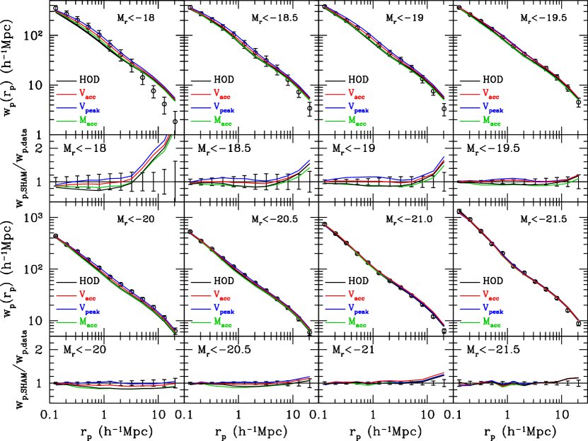
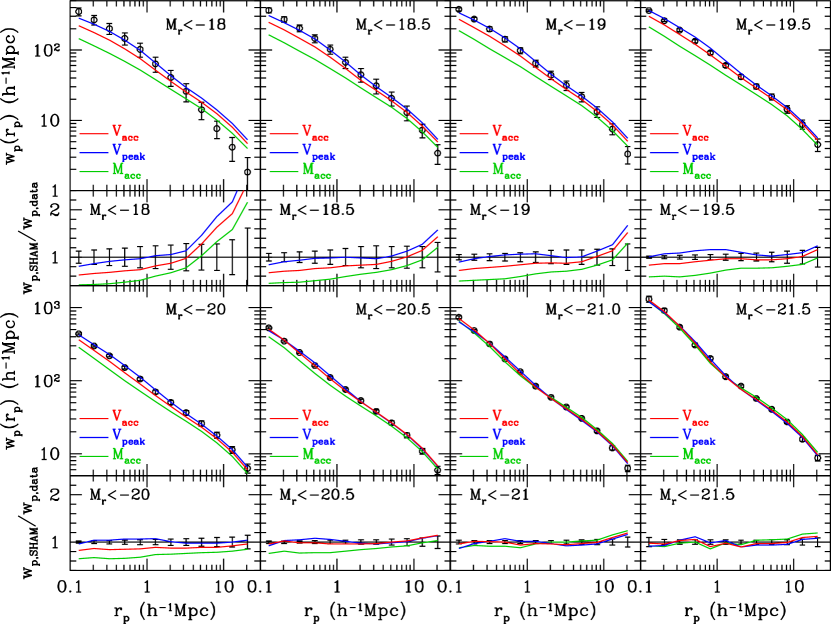
We first compare the modelling results from the three SHAM models (based on $M_{\rm acc}$, $V_{\rm acc}$, and $V_{\rm peak}$, respectively) including scatters as described in §2.2. Fig. 2 shows the best-fitting SHAM models to $w_{p}(r_{p})$ for the eight volume-limited luminosity threshold samples in SDSS DR7. The different SHAM models are shown as the different colour lines. Overall, the $V_{\rm peak}$ model seems to provide the best descriptions for all the galaxy samples, consistent with the conclusions of Reddick et al. (2013). The $M_{\rm acc}$ and $V_{\rm acc}$ models significantly underestimate the small-scale clustering for faint galaxies of threshold luminosity $M_{r}$ fainter than $-20.5$. This can be attributed to the shallower subhalo distribution profiles (Fig. 1). The $V_{\rm peak}$ model provides better fittings to the data, because the values of $V_{\rm peak}$ for subhaloes are usually much larger than $V_{\rm acc}$. We note that in Fig. 1 the red and blue curves for $V_{\rm acc}$ and $V_{\rm peak}$ are selected using the same thresholds. For the same galaxy sample, the thresholds of $V_{\rm acc}$ and $V_{\rm peak}$ would be different, and the density profiles for the subhaloes selected using the best-fitting $V_{\rm peak}$ model is closer to the dark matter distribution than using the best-fitting $V_{\rm acc}$ model.

Figure 8: Mean halo occupation functions of the best-fitting HOD and SCAM models from fitting the $w_{p}$–only data for different luminosity threshold samples.

Figure 9: Comparisons of the model parameters of the four models from fitting the $w_{p}$–only data for the different luminosity threshold samples. The left-hand panel shows the comparisons of the characteristic cutoff mass $M_{\rm min}$ of host haloes and the characteristic mass $M_{1}$ of haloes hosting on average one satellite galaxy. The satellite fraction $f_{\rm sat}$ is shown in the right-hand panel.

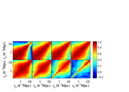
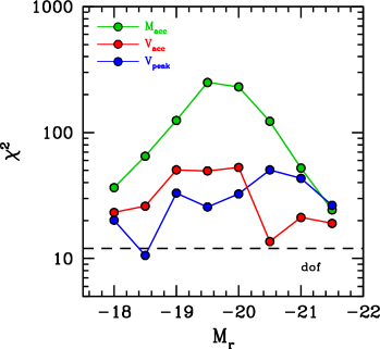
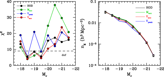
However, the goodness of fit to the data cannot be simply judged by eye, because the full covariance matrices of the measurements need to be taken into account. Each panel of Fig. 3 denotes the normalized covariance matrix for the corresponding 2PCF measurements shown in Fig. 2. The best-fitting $\chi^{2}$ for each model is displayed in Fig. 4. For example, from Fig. 2, it seems that the $V_{\rm acc}$ model fits slightly better than the $V_{\rm peak}$ model for the $M_{r}<-19.5$ sample. But the best-fitting $\chi^{2}$ value of the $V_{\rm peak}$ model is in fact smaller due to the strong positive correlation in the neighbouring bins of the data measurements. The large off-diagonal terms of the covariance matrix are important for all the galaxy samples except for the most luminous one.

As shown in Fig. 2 and Fig. 4, none of the three SHAM models can provide satisfactory fits for all galaxy samples. The $V_{\rm peak}$ model fits better for galaxy samples fainter than $-21$, while the $V_{\rm acc}$ model fits better for more luminous galaxy samples. The overall goodness-of-fit for the $V_{\rm peak}$ model is around $\chi^{2}/\rm{dof}\sim 3$. Therefore, the three SHAM models considered above can hardly be regarded as good models to the observed galaxy projected 2PCFs. We thus consider the more sophisticated and flexible subhalo models (SCAM) in the following section.

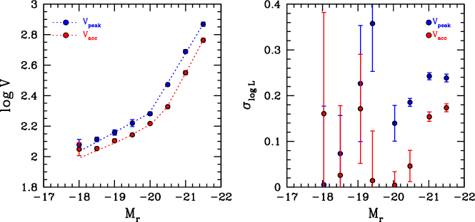
We show in the left panel of Fig. 5 the comparisons of the characteristic cutoff circular velocity and the inferred scatters in galaxy luminosity in haloes with the cutoff circular velocity in the $V_{\rm acc}$ and $V_{\rm peak}$ models, respectively. The more luminous galaxy samples have higher cutoff velocities, and the inferred cutoff for $V_{\rm peak}$ is generally about 0.1 dex higher than that for $V_{\rm acc}$.

As discussed in §2.2, the scatter $\sigma_{\log L}$ in galaxy luminosity at fixed circular velocity is encoded in the $\sigma_{\log V}$ parameter (width of the cutoff profile in the galaxy occupation function). Following Zheng et al. (2007) (see details in their Eq. 4), we have $\sigma_{\log L}=p\,\sigma_{\log V}/\sqrt{2}$, where $p$ is the local power-law slope of the $L$–$V$ relation, i.e. $p\equiv d\log L/d\log V$. To obtain the local power-law slope, we make use of the formula proposed by Vale & Ostriker (2006) to fit the relation between the sample luminosity threshold $L$ and the velocity cutoff $V$, ($V_{\rm acc}$ or $V_{\rm peak}$),

$$L=L_{0}\frac{(V/V_{t})^{a}}{\left[1+(V/V_{t})^{bk}\right]^{1/k}}.$$ (9)

The variables $L_{0}$, $V_{t}$, $a$, $b$ and $k$ are the model parameters. As seen from the left panel of Fig. 5, $L$–$V$ can also be well described by broken power laws, which justifies the use of local power-law slope $p$ in the above equation. The resulting scatter $\sigma_{\log L}$ is shown in the right panel of Fig. 5. Most scatters are smaller than 0.3, and the scatters in the $V_{\rm peak}$ model are generally larger. We note that the uncertainties on the scatters of the faint galaxy samples are very large. If the scatters are not taken into account in the SHAM models, only low-luminosity samples can be reasonably fitted. The scatters become important for luminous galaxies of $M_{r}<-20.5$. Overall the scatter we infer is consistent with that in the Tully-Fisher relation.

4.2 Results from the SCAM and HOD Models

The large $\chi^{2}/\rm{dof}$ values of the SHAM models are mostly caused by the underestimates of the small-scale clusterings. Since the small-scale galaxy pairs are dominated by the one-halo term, i.e. intra-halo galaxy pairs, the above underestimate could be an indication that subhaloes are not complete in representing satellite galaxies towards the centre of host haloes. Compared to the stellar components of satellite galaxies, subhaloes in $N$-body simulations are more easily disrupted, especially in the central regions of the host haloes where the tidal stripping effect is more significant. Indeed, the differences in the distribution profiles between subhaloes and satellite galaxies have been seen from $N$-body and hydrodynamic simulations of the same initial conditions (e.g. Fig. 7 of Weinberg et al. 2008 and Fig. 2 of Vogelsberger et al. 2014b).

However, if we work under the implicit assumption adopted in most SHAM models that satellites can only reside in subhaloes identified in $N$-body simulations, there is another way to improve the small-scale clustering fitted by adding additional components to the SHAM models. If we allow the central and satellite galaxies to have different occupation distributions in the distinct haloes and subhaloes as in our SCAM models, the deficiency of small-scale galaxy pairs can be compensated by more satellite galaxies populating subhaloes in lower mass host haloes. The galaxy number density can still be preserved by increasing the cutoff mass (or velocity) scale of the central galaxies. This seems like an extreme model that possibly artificially increases the fraction of the satellite galaxies, as we allow the relation between central galaxies and distinct haloes and that between satellites and subhaloes to be completely independent of each other in SCAM, which may not be true in reality. But on the other hand, there is some evidence that the connections of central and distinct haloes and those of satellite and subhaloes should be different (Yang et al., 2009; Yang et al., 2012; Neistein et al., 2011b; Rodríguez-Puebla et al., 2012; Wetzel et al., 2012; Watson & Conroy, 2013). Within the SHAM framework, results from our SCAM model that jointly fits the 2PCFs and the galaxy number density may serve as a probe to the difference between central and satellite galaxies.

The best-fitting HOD and SCAM models to the projected 2PCF $w_{p}$ are shown as the solid lines in Fig. 6. The $\chi^{2}$ of the model fittings are displayed in the left panel of Fig. 7. All the three SCAM models have much better best-fitting $\chi^{2}$ than the SHAM models, with only three more free parameters. Judged from the best-fitting $\chi^{2}$ values, the HOD model and the $V_{\rm acc}$ model are the two best models. For galaxy samples fainter than $M_{r}=-20$, the values of $\chi^{2}/{\rm dof}$ of the two models are both around unity. For more luminous galaxies, the HOD model has a $\chi^{2}/{\rm dof}\sim 1.8$. Note that in the HOD model, we set a prior by fixing the high mass end slope $\alpha$ of the satellite mean occupation function to be unity, for the purpose of reducing the number of parameters to be the same as in the SCAM models. If we also allow $\alpha$ to vary, the best-fitting value of $\alpha$ for these luminous galaxies is about $1.15$ and the $\chi^{2}/\rm{dof}$ would be significantly reduced to values around unity for the HOD model, as shown in table 2 of G15. Compared to $\alpha=1$, the higher-than-unity value of $\alpha$ implies that luminous satellite galaxies tend to populate even more massive haloes. We also note that due to the strong correlation in the off-diagonal elements of covariance matrices, the $\chi^{2}$ cannot be simply judged from the ratios between the models and data, as explained in the previous sections. For example, for the faint galaxy sample of $M_{r}<-19$, the HOD and $V_{\rm acc}$ model has almost the same $\chi^{2}$. However, the model predictions for $w_{p}$ are quite different.

Except for the $V_{\rm peak}$ model that has a strong variation of $\chi^{2}$ with the sample luminosity, all other three models can fit the faint galaxy samples very well. That is, once we allow the central and satellite galaxies to have different relations to the host haloes and the subhaloes, the satellite occupation can be adjusted to reproduce the small-scale clustering. For the most luminous galaxy sample of $M_{r}<-21.5$, all the four models have similar best-fitting $\chi^{2}$ values. As will be shown in the following, the ratio between the typical subhalo and the host halo mass is increasing with the galaxy luminosity (see e.g. Guo et al., 2014). According to Fig. 1, this makes the spatial distribution of subhaloes in the host haloes approach that of the dark matter, which explains why the SCAM models produce best-fitting $\chi^{2}$ values more consistent with the HOD model.

The right panel of Fig. 7 shows the best-fitting galaxy number density for the different models. The $V_{\rm peak}$ model has slightly lower galaxy number densities for the two samples of $M_{r}<-19$ and $M_{r}<-20$, mainly responsible for the larger $\chi^{2}$ shown in the left panel. All other three models reproduce the observed galaxy number densities remarkably well. We note that different from the SHAM models, in the SCAM models, the number densities of the models are not required to exactly match those of the galaxy samples, and the discrepancies in the number densities contribute to the total $\chi^{2}$. The models tend to find the balance between fitting the 2PCFs and fitting the sample number densities. However, the contribution of the number density to the total $\chi^{2}$ is usually small, since a reasonable model that describes well the 2PCFs also predicts a reasonable sample number density. Even for the case with the largest deviation seen in the right panel of Fig. 7 (the $V_{\rm peak}$ model for the sample of $M_{r}<-19$), its contribution to the total $\chi^{2}$ is only 3.7%.

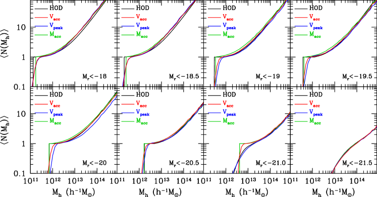
Fig. 8 shows the mean occupation functions of the best-fitting HOD and SCAM models. The sharp cutoff profiles are shown for the faint galaxy samples. But we should note that the scatters between the galaxy luminosity and the halo properties are not well constrained in all models for faint galaxies (see also G15). The cutoff profiles in the $V_{\rm acc}$ and $V_{\rm peak}$ models are softened because of the scatter between the circular velocity and the halo mass (see also Fig. 5 of Conroy et al., 2006). The trends in the mean occupation function with galaxy luminosity in different models are similar. For the $M_{r}<-21.5$ sample, the mean occupation functions from the four models are closely matched, while the differences become larger for fainter galaxies.

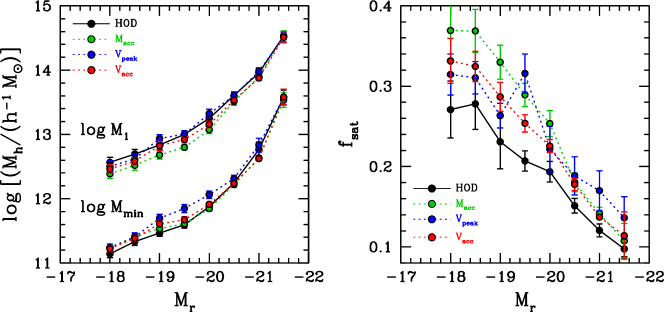
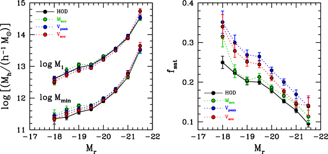
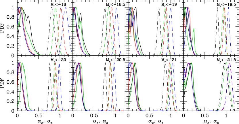
Fig. 9 presents the detailed comparisons of the three HOD parameters, the characteristic host halo mass $M_{\rm min}$, the characteristic mass of haloes hosting on average one satellite galaxy $M_{1}$ and the satellite fraction $f_{\rm sat}$. For the purpose of fair comparisons, we convert the corresponding model parameters in the SCAM models to those of the HOD model using Eq. 6 and the corresponding version for $V_{\rm acc}$ and $V_{\rm peak}$. Except for the $V_{\rm peak}$ model, all the other three models have consistent constraints to the host halo mass scale $M_{\rm min}$, because $M_{\rm min}$ is mostly constrained by the sample number density and the large-scale galaxy bias.

As seen in Fig. 1, the subhalo distribution profile in the host haloes is generally shallower than that of the dark matter distribution. The small-scale clustering is sensitive to the satellite occupation distribution, since it is dominated by the one-halo term, i.e. the galaxy pairs within the same host halo. In order to compensate the shallower profile and to match the small-scale clustering measurements of $w_{p}$, the SCAM models tend to populate satellite galaxies into lower mass haloes than in the HOD model. In the SCAM models, this is realized by lowering the mass (velocity) scale and increasing the scatter for populating subhaloes, compared to the way of populating distinct haloes. As a consequence, the characteristic mass $M_{1}$ (left panel of Fig. 9) inferred from the SCAM models is generally smaller and the satellite fraction $f_{\rm sat}$ (right panel of Fig. 9) is higher than that from the HOD model.

Figure 10: Similar to Fig. 2, but for the redshift-space monopole (circles) and quadrupole (squares) moments predicted by the SHAM models that best fit $w_{p}$ only. The measured and modelled monopole moments are shifted upwards by 30 for clarity.

Figure 11: Similar to Fig. 6, but for the bestfitting HOD and SCAM models of fitting both the projected and redshift-space 2PCFs.

Figure 12: Similar to Fig. 10, but for the HOD and SCAM models. The bestfitting models come from jointly fitting the projected 2PCF $w_{p}$ and redshift-space 2PCF multiple moments $\xi_{0/2/4}$. The measurements of the monopole moments are shifted upward by 10 for clarity.

Figure 13: Similar to Fig. 7, but for models jointly fitting the projected and redshift-space 2PCFs.

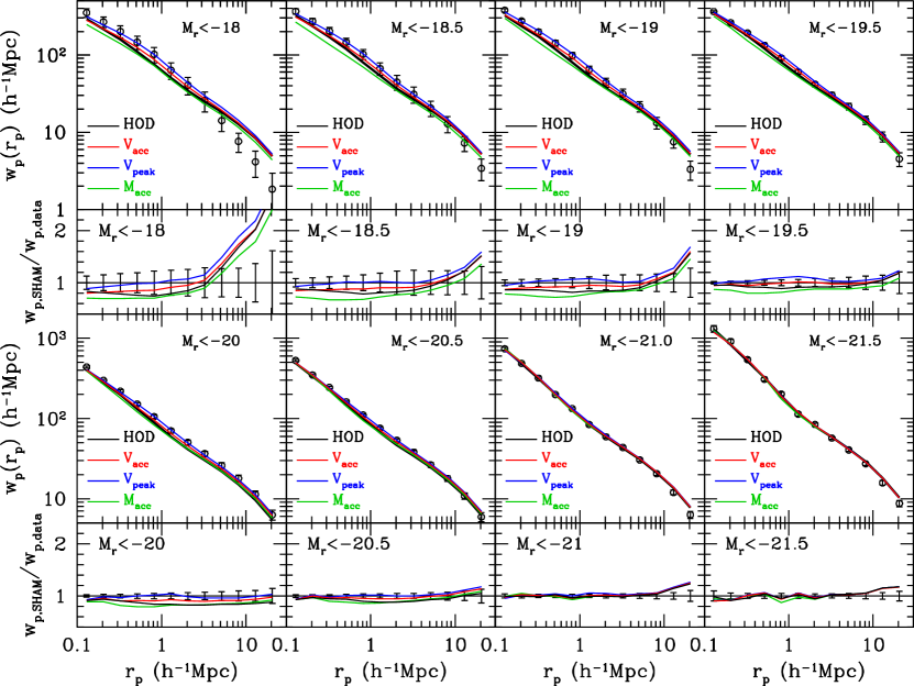
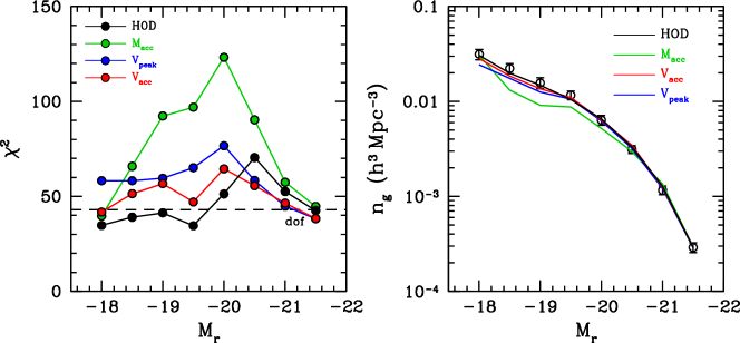
The $V_{\rm acc}$ SCAM model shows the best overall agreement with the HOD model, with more or less consistent best-fitting $\chi^{2}$ values (Fig. 7). The HOD-related parameters of the four models have better agreement for luminous galaxies. However, the $\chi^{2}$ values are still quite different from model to model (Fig. 7), indicating the effect and importance of the spatial distribution of satellites (subhaloes or particles in the four models) in modelling small-scale $w_{p}$. For example, the model parameters of the three subhalo models for the $M_{r}<-20.5$ sample are consistent with each other, but the $M_{\rm acc}$ model still has a $\chi^{2}/{\rm dof}$ value as large as 4.2. Based on the best-fitting $\chi^{2}$ values, the subhaloes selected by circular velocities ($V_{\rm acc}$ or $V_{\rm peak}$) seem to better trace the satellite galaxies (see also e.g. Chaves-Montero et al., 2015).

5 Modelling the Redshift-space 2PCFs

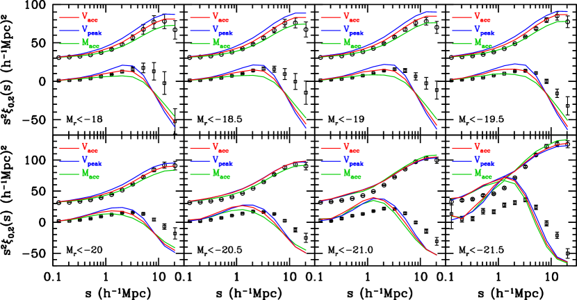
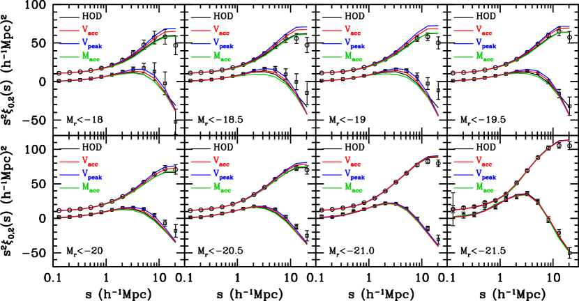
As shown in G15, jointly fitting the projected and redshift-space 2PCFs helps tighten the constraints to the galaxy spatial distribution in the haloes, as well as constraining their velocity distributions. Since the traditional SHAM models do not have galaxy velocity bias that are required to fit the redshift-space 2PCFs, the resulting $\chi^{2}/\rm{dof}$ values are found to be significantly large. We show in Fig. 10 the predicted redshift-space monopole and quadrupole moments in the SHAM models that bestfit $w_{p}$. Clearly, the traditional SHAM models fail to describe the redshift-space clustering, especially the quadrupoles. Therefore, in this section, we only compare the HOD and SCAM model fitting results. We first display in Fig. 11 the predictions of the projected 2PCF $w_{p}(r_{p})$ for the bestfitting HOD and SCAM models from jointly fitting both the projected and redshift-space 2PCFs. It is similar to Fig. 6, except that the $M_{\rm acc}$ model leads to poorer fits for the faint galaxy samples, as a result of tuning parameters to fit the redshift-space clustering. Fig. 12 shows the best fits to the redshift-space 2PCFs. For clarity, we only show the best-fitting models to the measured redshift-space monopole (circles) and quadrupole (squares) moments. The hexadecapole moments are also used in the model fittings, but not shown in the figure. The $\chi^{2}$ of the best-fitting models are shown in the left panel of Fig. 13, while the right panel displays the best-fitting sample number densities.

Figure 14: Similar to Fig. 9, but for the models jointly fitting the projected and redshift-space 2PCFs.

Figure 15: Galaxy velocity bias probability distributions for different models, constrained from jointly fitting the projected and redshift-space 2PCFs. The solid and dashed lines are for the central ($\alpha_{c}$) and satellite ($\alpha_{s}$) galaxy velocity bias, respectively. Different panels show the distributions for different luminosity threshold samples. The black, green, blue and red curves are for the HOD, $M_{\rm acc}$, $V_{\rm peak}$ and $V_{\rm acc}$ models, respectively.

Except for the $M_{\rm acc}$ model, all other three models fit the data reasonably well. As seen from Fig. 12, the largest deviation of the $M_{\rm acc}$ model fits from the measurements and from the fits of other models lies in the quadrupole, which dominates contributions to the $\chi^{2}$. Moreover, the best-fitting sample number densities from the $M_{\rm acc}$ model are significantly lower than the observed ones for the faint galaxy samples (except for the $M_{r}<-18$ sample). Compared to the constraints from fitting $w_{p}$ only (Fig. 7), the $M_{\rm acc}$ model has the galaxy number density decreased in the joint-fitting in order to match the redshift-space clustering. Since the $M_{\rm acc}$ model provides very good fittings to $w_{p}$ for the faint galaxies, the failure in matching the galaxy redshift-space clustering measurements indicates that the subhaloes selected based on $M_{\rm acc}$ cannot reproduce well the velocity distribution of the satellite galaxies in the observation.

Except for the sample of $M_{r}<-20.5$, the HOD model can explain the observed galaxy 2PCFs very well, with a reasonable $\chi^{2}/{\rm dof}$ for each sample. As mentioned in the previous section, the model fitting to the luminous galaxy samples (including $M_{r}<-20.5$) can be significantly improved when we allow the high-mass end slope $\alpha$ of the mean occupation function to vary (see e.g. Table 2 of Guo et al., 2015c). Among the three SCAM models, the $V_{\rm acc}$ model better fits the data than the other two subhalo models, similar to the case of fitting $w_{p}$ only. The dof of the models is 43 (48 2PCF data points plus one number density and minus six free parameters), and the 2$\sigma$ range of the expected $\chi^{2}$ distribution is about $43\pm 18.5$. Even though the $\chi^{2}$ values from the HOD model are overall lower than those from the subhalo models, those from the $V_{\rm acc}$ and $V_{\rm peak}$ models are still within the 2$\sigma$ range, giving reasonable fits to the data.

Fig. 14 shows comparisons of the parameters of $M_{1}$, $M_{\rm min}$ and $f_{\rm sat}$, as in Fig. 9. Similar to the results from fitting $w_{p}$ only, differences in $M_{\rm min}$ and $M_{1}$ from different models become larger for fainter galaxy samples. If we focus on comparing the HOD model and the $V_{\rm acc}$ and $V_{\rm peak}$ subhalo models (that provide reasonable fits to the data), we find that the HOD model has the smallest $M_{\rm min}$ and highest $M_{1}$ values, and the lowest satellite fraction. The SCAM models tend to populate satellite galaxies into lower mass haloes to compensate their shallower spatial distribution in the host haloes. Compared to the right panel of Fig. 9, the uncertainties in $f_{\rm sat}$ are greatly reduced, because the redshift-space clustering puts more constraints on the satellite galaxy distributions.

Figure 16: Projected number density profile for satellite galaxies from the four different bestfitting models. Offsets are added to separate the cases of different luminosity threshold samples for clarity.

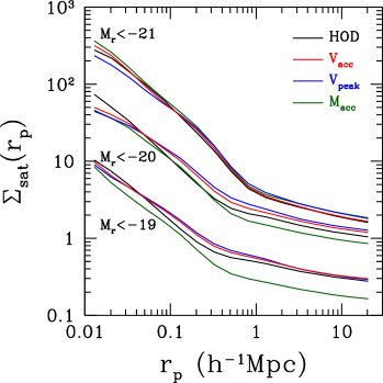
We show in Fig. 15 the model constraints to the galaxy velocity bias parameters for the different luminosity threshold samples. The black, green, blue and red curves are for the HOD, $M_{\rm acc}$, $V_{\rm peak}$ and $V_{\rm acc}$ models, respectively. The solid and dashed lines are for the central ($\alpha_{c}$) and satellite ($\alpha_{s}$) galaxy velocity bias parameters, respectively. The model constraints for the central galaxy velocity bias are generally consistent with each other. The best-fitting $\alpha_{c}$ values are much smaller than those in G15. The difference is caused by the different reference to define the velocity bias. In this paper, the reference halo velocity is defined as the average particle velocities within inner 10% halo radius (core), while the velocity bias $\alpha_{c}$ in G15 is with respect to the halo bulk velocity. There is a relative motion between the core and bulk of a halo (Behroozi et al., 2013). An average central galaxy velocity bias $\alpha_{c}\sim 0.1$ is required to fit the redshift-space 2PCFs.

For the satellite velocity bias $\alpha_{s}$, the results from the HOD and the SCAM models cannot be directly compared. The satellite velocity bias $\alpha_{s}$ for the HOD model is defined with respect to the dark matter velocity dispersions within the haloes, i.e. $\alpha_{s,\rm{HOD}}=\sigma_{\rm sat}/\sigma_{v}$, while the satellite velocity bias in the SCAM models is with respect to the velocity dispersions of the subhaloes in the host haloes, i.e. $\alpha_{s,\rm{SCAM}}=\sigma_{\rm sat}/\sigma_{\rm sub}=(\sigma_{\rm sat}/\sigma_{v})/(\sigma_{\rm sub}/\sigma_{v})=\alpha_{s,\rm{HOD}}/\alpha_{\rm sub}$. The subhalo velocity bias $\alpha_{\rm sub}$ is measured to vary from $1.02$ to $1.11$ in §3. We take a medium value of $1.07$ for $\alpha_{\rm sub}$. So we can directly compare $\alpha_{s,\rm{HOD}}$ and $\alpha_{\rm sub}\alpha_{s,\rm{SCAM}}$. The value of $\alpha_{s,\rm{HOD}}$ is around $0.8$ for faint galaxies, and increases with luminosity for the two most luminous galaxy samples, consistent with the results of G15. But $\alpha_{s,\rm{HOD}}$ is always smaller than $\alpha_{s,\rm{SCAM}}$ (hence even smaller than $\alpha_{\rm sub}\alpha_{s,\rm{SCAM}}$) inferred from the three SCAM models. There are also significant differences in $\alpha_{s,\rm{SCAM}}$ among the three SCAM models, with the $M_{\rm acc}$ model having the smallest $\alpha_{s,\rm{SCAM}}$ and the $V_{\rm peak}$ model having the largest. The results manifest that models with a shallower satellite spatial distribution need a compensation of having more satellites in lower mass haloes and a larger boost in velocity dispersion to match the redshift-space distortion, consistent with the test shown in Fig. 11 of Guo et al. (2015a).

Figure 17: Comparisons of the subhalo model parameters for the central and satellite galaxies from jointly fitting the projected and redshift-space 2PCFs. The left panel shows the comparisons of the circular velocity thresholds $V_{\rm min,cen}$ and $V_{\rm min,sat}$ for the $V_{\rm acc}$ (open circles with solid line) and $V_{\rm peak}$ (filled circles with dashed line) models. The right panel shows the comparisons of the scatters $\sigma_{\log V_{\rm cen}}$ and $\sigma_{\log V_{\rm sat}}$ for the $V_{\rm acc}$ model only. See text for details.

Satellites in the HOD model have the steepest spatial distribution profile. Subhaloes in the $M_{\rm acc}$ model have steeper density profile than those in the other two subhalo models. We show in Fig. 16 three examples for the projected satellite galaxy number density profiles $\Sigma_{\rm sat}(r_{p})$ as a function of the projected distance $r_{p}$ to centres of hosting haloes (see e.g. Chen et al., 2006; Wang et al., 2014). The projected number density is integrated over the same line-of-sight distance as in the calculation of $w_{p}(r_{p})$, i.e. $40\,h^{-1}{\rm{Mpc}}$. The turnover points in each sample roughly show the scale of the virial radii of the hosting haloes in these samples. The trend of the satellite density profiles is consistent with the behaviour of satellite velocity bias $\alpha_{s}$ in Fig. 15. Although the $M_{\rm acc}$ model generally has a slope of the satellite galaxy density profile closer to the dark matter distribution, it does not necessarily lead to better fits to the galaxy 2PCF measurements. The difference in the different subhalo models is not only in the resulting subhalo density profiles, but also in the different hosting halo masses (left panel of Fig. 14). The difference in the satellite density profiles is partly compensated by the different satellite fraction $f_{\rm sat}$ in each model. The $V_{\rm peak}$ model has the highest $f_{\rm sat}$ in each galaxy sample (right panel of Fig. 14) to compensate for its shallowest satellite distribution profiles.

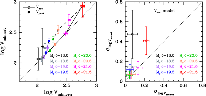
Since in our subhalo models we allow the central and satellite galaxies to have different relations with the hosting haloes (subhaloes), we can compare the model parameters for the central and satellite galaxies. Since the $M_{\rm acc}$ model does not have a good best-fitting $\chi^{2}$ for each galaxy sample, we focus on the comparisons between the $V_{\rm acc}$ and $V_{\rm peak}$ models. The left panel of Fig. 17 shows the comparisons of the circular velocity thresholds $V_{\rm min,cen}$ and $V_{\rm min,sat}$ for the $V_{\rm acc}$ (open circles with solid line) and $V_{\rm peak}$ (filled circles with dashed line) models. It is clear that the assumption of the same galaxy–halo relation for central and satellite galaxies does not hold for the $V_{\rm peak}$ model, where $V_{\rm min,sat}$ is generally much larger than $V_{\rm min,cen}$. However, the $V_{\rm acc}$ model has almost the same circular velocities for central and satellite galaxies. The relation that $V_{\rm min,cen}=V_{\rm min,sat}$ holds within errors for all the luminosity threshold samples.

The right panel of Fig. 17 shows the scatter parameter $\sigma_{\log V_{\rm acc}}$ in the $V_{\rm acc}$ model for distinct haloes and subhaloes (corresponding to central and satellite galaxies). In general, the scatters for the central and satellite galaxies are not equal to each other, with the satellite galaxies having larger scatters between the luminosity and $V_{\rm acc}$. For the three luminosity threshold samples around $L_{*}$, i.e. $M_{r}<-20$, $-20.5$ and $-21$, central and satellite galaxies have similar $V_{\rm min,acc}$ and $\sigma_{\log V_{\rm acc}}$. It implies that the SHAM model with scatter works well for these samples, which is consistent with the low $\chi^{2}$ values in the $V_{\rm acc}$ model of $w_{p}$-only data in Fig. 4. But for other samples, central and satellite galaxies have different scatters in the luminosity-velocity relation, with satellites having larger scatters, which may be interpreted as resulted from the different evolution histories of the central and satellite galaxies.

We note that the $V_{\rm peak}$ model generally has a higher $V_{\rm min,sat}$ than $V_{\rm min,cen}$, compared to the $V_{\rm acc}$ model. However, the $V_{\rm peak}$ model has a higher satellite fraction $f_{\rm sat}$ (right panel of Fig. 14), owing to a much larger satellite luminosity-velocity scatter ($\sigma_{\log V_{\rm peak,sat}}$) than in the $V_{\rm acc}$ model.

As a whole, when modelling redshift-space 2PCFs, we find that both the HOD and SCAM models can give reasonable fits to the measurements for luminous galaxy samples (above $L_{*}$). For low luminosity galaxy samples (below $L_{*}$), the HOD model, which use dark matter particles to represent satellite galaxies, leads to the lowest $\chi^{2}$ among all the models. Among the subhalo models, if the best-fitting $\chi^{2}$ values of low luminosity samples are compared, the $V_{\rm acc}$ model has the best performance. The $V_{\rm peak}$ model is somewhat worse, and the $M_{\rm acc}$ model just fails to fit the data (except for the $M_{r}<-18$ sample). The results imply that the circular velocities $V_{\rm acc}$ and $V_{\rm peak}$ are more correlated with satellite luminosity than $M_{\rm acc}$.

6 Conclusions and Discussions

In this paper, we employ the HOD model and different SHAM models (and the extension, the SCAM models) to model the projected and redshift-space 2PCF measurements for the different luminosity threshold samples in the SDSS DR7 Main galaxy sample. All the models are based on the high-resolution MDPL/SMDPL $N$-body simulations, using the accurate and efficient method developed in Zheng & Guo (2016). We explicitly compare the best-fitting $\chi^{2}$ values and the modelling results of the HOD model, the SHAM models, and the SCAM models. The HOD model uses dark matter particles in host haloes to represent satellite galaxies, while the three sets of SHAM/SCAM models use halo properties $M_{\rm acc}$, $V_{\rm acc}$, and $V_{\rm peak}$ to establish the connection between haloes and galaxies, respectively.

In the SHAM model, distinct haloes and subhaloes are treated in the same way when connected to galaxies. Even with the projected 2PCF $w_{p}$ data alone, the SHAM model, no matter which halo property is used, generally fails to provide satisfactory explanations to all the luminosity threshold samples, with a typical $\chi^{2}/{\rm dof}>2$. We therefore introduce the SCAM model by allowing the relation between central galaxies and distinct haloes and that between satellite galaxies and subhaloes to be different, and determine the model parameters by jointly fitting the observed 2PCFs and the sample number density. The SCAM models give significantly better $\chi^{2}$ than the SHAM models.

For an easy comparison, we choose parametrizations so that the HOD and SCAM models have the same dof. The main difference between the two models lies in the spatial distribution profile of satellites inside distinct haloes. Subhaloes (satellite tracers in the SCAM models) generally have a shallower spatial distribution profile than dark matter particles (satellite tracers assumed in our HOD model). The shallow distribution profile of subhaloes in $N$-body simulations may be partially an effect of ignoring the baryon components — satellites traced by the more tightly bounded stellar component are less suffered from tidal disruption that destructs a fraction of subhaloes near the halo centre. This is supported by the comparisons of distributions of subhaloes and satellite galaxies in hydrodynamic and $N$-body simulations (e.g. Weinberg et al., 2008; Vogelsberger et al., 2014a), and additional investigations along such a direction can shed further light on such a phenomenon. In this paper, we work under the SHAM assumption that satellites are traced by subhaloes and investigate to what extent the subhalo models can interpret the data and to study the corresponding implications.

As expected, the differences in the modelling results between the HOD and SCAM models and among the different SCAM models can be largely traced back to the differences in the spatial distribution profile of satellites. Compared to the HOD modelling results, the SCAM models tend to populate more satellites into lower mass host haloes to compensate the shallower subhalo distribution profile and hence to fit the small-scale clustering measurements. This leads to higher satellite fraction in the SCAM models. When fitting the redshift-space 2PCFs, we include the central and satellite galaxy velocity biases in all the models. The derived nonzero central galaxy velocity bias constraints of the SCAM models are consistent with the HOD model. The satellite galaxy velocity bias is higher in the SCAM models. The reason is as follows. As mentioned above, to match the small-scale (real-space) clustering, more satellites are populated into lower mass haloes in the SCAM models, and in these host haloes satellite moves more slowly than in the HOD model. The SCAM models therefore need to boost the velocities of satellites inside host haloes to fit the redshift-space distortion in the data, especially the Finger-of-God part.

From jointly modelling the projected and redshift-space 2PCFs, we find that the HOD model has an overall good performance. For luminous samples (above $L_{*}$), all SCAM models provide good fits to the data, and the $V_{\rm peak}$ and $V_{\rm acc}$ models even work better than the HOD model in terms of $\chi^{2}$ (Fig. 13). However, for galaxy samples with threshold luminosity below $L_{*}$, the models become divided. The HOD model is superb, with the lowest $\chi^{2}$ values. The $M_{\rm acc}$ model fails to fit the data (except for the sample with the lowest luminosity threshold, $M_{r}<-18$). The $V_{\rm acc}$ and $V_{\rm peak}$ models lead to $\chi^{2}$ values higher than those from the HOD model, with the $V_{\rm acc}$ model being better. The $\chi^{2}$ values from the two models are within the 2$\sigma$ range of the expected value. The results suggest that circular velocities ($V_{\rm acc}$ and $V_{\rm peak}$) are better quantities than mass $M_{\rm acc}$ to connect to luminosity of galaxies, especially satellites, even though $M_{\rm acc}$-selected subhaloes have the steepest spatial profile among the SCAM models. We therefore recommend that the SHAM model should no longer use $M_{\rm acc}$ to link to galaxy luminosity. This is in line with the recent finding by Contreras et al. (2015), who investigate the SHAM performance for galaxies in two different galaxy formation models and find that subhalo mass is not a good indicator of galaxy properties. For the two circular velocity SCAM models, the $V_{\rm acc}$ model is slightly better than the $V_{\rm peak}$ model in reproducing the projected and redshift-space 2PCFs. In either model, different galaxy–halo relations for central and satellite galaxies (distinct haloes and subhaloes) are overall required by the data.

The comparisons between the best-fitting $\chi^{2}$ for the HOD and SCAM models show that the HOD model is generally the best model to describe the galaxy distribution in both projected and redshift spaces. However, the $V_{\rm acc}$ and $V_{\rm peak}$ models are still acceptable, especially to model luminous galaxy samples. Including other clustering statistics (e.g. the three-point correlation functions; Guo et al. 2015b) may help to further distinguish these models, as well as to tighten parameter constraints.

It is worth noting that we adopt specific functional forms (Equations 2 and 5) to describe the occupation functions of central and satellite galaxies in the haloes for all the models considered in this paper. Such a functional form is motivated by the results in the semi-analytic models and hydrodynamic simulations of galaxy formation (Zheng et al., 2005). It can be derived by assuming a lognormal distribution of the central galaxy luminosity at fixed halo mass and a power-law relation between the mean luminosity of central galaxies and the host halo mass (Zheng et al., 2007). In the halo mass range where the luminosity-halo mass relation (LHMR) or SHMR deviates significantly from a power law, the functional form is less accurate and the interpretation of parameters like $M_{\rm min}$ becomes subtle. Leauthaud et al. (2011) compared the difference between the bestfitting HOD parameter $M_{\rm min}$ (defined as $\langle N_{\rm cen}(M_{\rm min})\rangle=0.5$) with the SHMR of Behroozi et al. (2010) and that with a power law SHMR, and found that the difference in $M_{\rm min}$ is $<20\%$ for models with $M_{\rm min}$ in the range of $10^{12}$–$10^{14}M_{\odot}$. For the relevant samples we model, the changes in $\log M_{\rm min}$ are 0.08, 0.04, and -0.04 dex for $M_{r}<-20.5$, $-21$, and $-21.5$, repectively, all within the 1$\sigma$ model uncertainties.

To derive the functional form of Equation 2, the scatter in central galaxy luminosity needs to be independent of halo mass and $\sigma_{\log M_{\rm h}}$ is connected to the luminosity scatter and the form of LHMR. In general, $\sigma_{\log M_{\rm h}}$ should not be interpreted as the scatter of halo mass at fixed galaxy luminosity (Zheng et al., 2007; Leauthaud et al., 2011). Instead, it describes the width of the cutoff profile of the central galaxy mean occupation function, as noted in Section 2.2. In modelling the data, the role of the cutoff profile is to convolve with halo mass function and halo bias factor to try to reproduce the galaxy number density and the large-scale galaxy bias, and the two quantities are not sensitive to the functional form of the cuttoff profile (as long as the freedoms in width and mass scale are included). Therefore, while the interpretation of the parameters like $\sigma_{\log M_{\rm h}}$ can be subtle, the modelling results would not be affected much by the functional form.

In the implementation of the HOD model, we make the assumption that satellite galaxies follow the spatial distribution of the dark matter inside haloes. Although this assumption is commonly adopted in HOD modelling of galaxy clustering and is loosely motivated by theoretical studies (e.g. Nagai & Kravtsov, 2005), it needs to be further tested. In hydrodynamic galaxy formation models, the spatial profile of satellite galaxies depends on the implementation details. For example, stellar mass loss can be different for satellites in models with galactic winds of different strengths (e.g. Simha et al., 2012), leading to differences in the spatial distribution profile of satellites for a given stellar mass threshold (or galaxy number density). Given such uncertainties, in modelling galaxy clustering, one can introduce freedom in satellite spatial profile and galaxy formation models can help inform the sensible parametrization of such a profile.

More generally, comparison of the spatial distributions of satellites, dark matter, and subhaloes in hydrodynamic and $N$-body simulations can also help to evaluate the limitations of each model, to improve the prescriptions of each model, and to choose the best one to model the clustering for a given sample of galaxies. The validity of the SHAM method can also be tested with such simulations. Simha et al. (2012) applied the SHAM model (with $M_{\rm acc}$ as the halo/subhalo variable) to collisionless $N$-body simulations and compared with the galaxies in corresponding hydrodynamic simulations (with the same initial conditions). They find good agreement for the HODs and satellite distribution profiles for galaxy samples defined by thresholds in stellar mass. They also find that SHAM slightly overpopulates massive haloes and hence overpredicts the small-scale clustering, which is attributed to stellar mass loss of satellite galaxies. The trend seems to be opposite to our results, although the details depends on the implementation in the strength of galactic winds. Chaves-Montero et al. (2015) also investigate the SHAM model with $N$-body and the hydrodynamical simulation (the EAGLE simulation) for stellar mass threshold galaxy samples, using various circular velocities as the halo/subhalo variables. They found that the peak circular velocity of a subhalo after relaxation, which is a modified version of the $V_{\rm peak}$ used in our models, correlates most strongly with the galaxy stellar mass. The SHAM model using this parameter shows better agreement with the galaxy clustering measurements in the hydrodynamic simulations. Further investigations following the above ones will be useful (e.g. for luminosity-threshold samples).

One basic assumption of the HOD model is that the statistical properties of the galaxy content in a halo only depend on the halo mass. Since the clustering of haloes of the same mass depends on the halo assembly history (e.g. Gao et al., 2005; Wechsler et al., 2006; Zhu et al., 2006; Jing et al., 2007), the above assumption means that the halo assembly effect is not translated into galaxy properties in haloes of the same mass. If the galaxy assembly effect exists (meaning that galaxy properties are correlated with halo assembly), it would possibly affect the HOD modelling (e.g. Zu et al., 2008; Zentner et al., 2014; Hearin et al., 2015; Paranjape et al., 2015) and the current HOD framework would then need to be extended. However, there is no definite conclusion yet on whether the assembly bias in galaxy properties shows up in hydrodynamic simulations (e.g. Berlind et al., 2003; Chaves-Montero et al., 2015) or in galaxy clustering measurements (e.g. Lin et al., 2016). According to the investigation by Chaves-Montero et al. (2015) with hydrodynamic simulations, modelling (with SHAM) based on certain circular velocity variable can capture about 50% of the assembly bias effect in galaxy clustering. Since the SCAM models with circular velocity we introduce in this paper are still less successful than the HOD model, it remains to be seen whether the galaxy assembly effect is significant in real data. In any case, further studies on galaxy assembly are necessary and we reserve such investigations for future work.

References

- Abazajian et al. (2009) Abazajian K. N., Adelman-McCarthy J. K., Agüeros M. A., et al. 2009, ApJS, 182, 543
- Behroozi et al. (2010) Behroozi P. S., Conroy C., Wechsler R. H., 2010, ApJ, 717, 379
- Behroozi et al. (2013) Behroozi P. S., Wechsler R. H., Wu H.-Y., 2013, ApJ, 762, 109
- Berlind & Weinberg (2002) Berlind A. A., Weinberg D. H., 2002, ApJ, 575, 587
- Berlind et al. (2003) Berlind A. A., et al., 2003, ApJ, 593, 1
- Blanton et al. (2005) Blanton M. R., et al., 2005, AJ, 129, 2562
- Bower et al. (2006) Bower R. G., Benson A. J., Malbon R., Helly J. C., Frenk C. S., Baugh C. M., Cole S., Lacey C. G., 2006, MNRAS, 370, 645
- Bryan & Norman (1998) Bryan G. L., Norman M. L., 1998, ApJ, 495, 80
- Chaves-Montero et al. (2015) Chaves-Montero J., Angulo R. E., Schaye J., Schaller M., Crain R. A., Furlong M., 2015, preprint, (arXiv:1507.01948)
- Chen et al. (2006) Chen J., Kravtsov A. V., Prada F., Sheldon E. S., Klypin A. A., Blanton M. R., Brinkmann J., Thakar A. R., 2006, ApJ, 647, 86
- Conroy et al. (2006) Conroy C., Wechsler R. H., Kravtsov A. V., 2006, ApJ, 647, 201
- Contreras et al. (2015) Contreras S., Baugh C. M., Norberg P., Padilla N., 2015, MNRAS, 452, 1861
- Croton et al. (2006) Croton D. J., et al., 2006, MNRAS, 365, 11
- Gao et al. (2004) Gao L., De Lucia G., White S. D. M., Jenkins A., 2004, MNRAS, 352, L1
- Gao et al. (2005) Gao L., Springel V., White S. D. M., 2005, MNRAS, 363, L66
- Guo et al. (2010) Guo Q., White S., Li C., Boylan-Kolchin M., 2010, MNRAS, 404, 1111
- Guo et al. (2011) Guo Q., et al., 2011, MNRAS, 413, 101
- Guo et al. (2013) Guo H., et al., 2013, ApJ, 767, 122
- Guo et al. (2014) Guo H., et al., 2014, MNRAS, 441, 2398
- Guo et al. (2015a) Guo H., et al., 2015a, MNRAS, 446, 578
- Guo et al. (2015b) Guo H., et al., 2015b, MNRAS, 449, L95
- Guo et al. (2015c) Guo H., et al., 2015c, MNRAS, 453, 4368
- Hearin et al. (2015) Hearin A. P., Watson D. F., van den Bosch F. C., 2015, MNRAS, 452, 1958
- Jing et al. (1998) Jing Y. P., Mo H. J., Börner G., 1998, ApJ, 494, 1
- Jing et al. (2007) Jing Y. P., Suto Y., Mo H. J., 2007, ApJ, 657, 664
- Klypin et al. (2016) Klypin A., Yepes G., Gottlöber S., Prada F., Heß S., 2016, MNRAS, 457, 4340
- Knebe et al. (2013) Knebe A., et al., 2013, MNRAS, 435, 1618
- Kravtsov et al. (2004) Kravtsov A. V., Berlind A. A., Wechsler R. H., Klypin A. A., Gottlöber S., Allgood B., Primack J. R., 2004, ApJ, 609, 35
- Leauthaud et al. (2011) Leauthaud A., Tinker J., Behroozi P. S., Busha M. T., Wechsler R. H., 2011, ApJ, 738, 45
- Leauthaud et al. (2012) Leauthaud A., et al., 2012, ApJ, 744, 159
- Lin et al. (2016) Lin Y.-T., Mandelbaum R., Huang Y.-H., Huang H.-J., Dalal N., Diemer B., Jian H.-Y., Kravtsov A., 2016, ApJ, 819, 119
- Moster et al. (2010) Moster B. P., Somerville R. S., Maulbetsch C., van den Bosch F. C., Macciò A. V., Naab T., Oser L., 2010, ApJ, 710, 903
- Nagai & Kravtsov (2005) Nagai D., Kravtsov A. V., 2005, ApJ, 618, 557
- Neistein et al. (2011a) Neistein E., Weinmann S. M., Li C., Boylan-Kolchin M., 2011a, MNRAS, 414, 1405
- Neistein et al. (2011b) Neistein E., Li C., Khochfar S., Weinmann S. M., Shankar F., Boylan-Kolchin M., 2011b, MNRAS, 416, 1486
- Nuza et al. (2013) Nuza S. E., et al., 2013, MNRAS, 432, 743
- Onions et al. (2012) Onions J., et al., 2012, MNRAS, 423, 1200
- Paranjape et al. (2015) Paranjape A., Kovač K., Hartley W. G., Pahwa I., 2015, MNRAS, 454, 3030
- Peacock & Smith (2000) Peacock J. A., Smith R. E., 2000, MNRAS, 318, 1144
- Planck Collaboration (2014) Planck Collaboration 2014, A&A, 571, A16
- Pujol et al. (2014) Pujol A., et al., 2014, MNRAS, 438, 3205
- Reddick et al. (2013) Reddick R. M., Wechsler R. H., Tinker J. L., Behroozi P. S., 2013, ApJ, 771, 30
- Rodríguez-Puebla et al. (2012) Rodríguez-Puebla A., Drory N., Avila-Reese V., 2012, ApJ, 756, 2
- Rodríguez-Puebla et al. (2013) Rodríguez-Puebla A., Avila-Reese V., Drory N., 2013, ApJ, 767, 92
- Rodriguez-Puebla et al. (2016) Rodriguez-Puebla A., Behroozi P., Primack J., Klypin A., Lee C., Hellinger D., 2016, preprint, (arXiv:1602.04813)
- Sawala et al. (2015) Sawala T., et al., 2015, MNRAS, 448, 2941
- Schaye et al. (2015) Schaye J., et al., 2015, MNRAS, 446, 521
- Simha et al. (2012) Simha V., Weinberg D. H., Davé R., Fardal M., Katz N., Oppenheimer B. D., 2012, MNRAS, 423, 3458
- Skibba et al. (2015) Skibba R. A., et al., 2015, ApJ, 807, 152
- Somerville et al. (2008) Somerville R. S., Hopkins P. F., Cox T. J., Robertson B. E., Hernquist L., 2008, MNRAS, 391, 481
- Springel et al. (2008) Springel V., et al., 2008, MNRAS, 391, 1685
- Tinker et al. (2005) Tinker J. L., Weinberg D. H., Zheng Z., Zehavi I., 2005, ApJ, 631, 41
- Vale & Ostriker (2006) Vale A., Ostriker J. P., 2006, MNRAS, 371, 1173
- Vogelsberger et al. (2014a) Vogelsberger M., et al., 2014a, MNRAS, 444, 1518
- Vogelsberger et al. (2014b) Vogelsberger M., et al., 2014b, Nature, 509, 177
- Wang et al. (2006) Wang L., Li C., Kauffmann G., De Lucia G., 2006, MNRAS, 371, 537
- Wang et al. (2007) Wang Y., Yang X., Mo H. J., van den Bosch F. C., 2007, ApJ, 664, 608
- Wang et al. (2014) Wang W., Sales L. V., Henriques B. M. B., White S. D. M., 2014, MNRAS, 442, 1363
- Watson & Conroy (2013) Watson D. F., Conroy C., 2013, ApJ, 772, 139
- Wechsler et al. (2006) Wechsler R. H., Zentner A. R., Bullock J. S., Kravtsov A. V., Allgood B., 2006, ApJ, 652, 71
- Weinberg et al. (2008) Weinberg D. H., Colombi S., Davé R., Katz N., 2008, ApJ, 678, 6
- Wetzel et al. (2012) Wetzel A. R., Tinker J. L., Conroy C., 2012, MNRAS, 424, 232
- White & Rees (1978) White S. D. M., Rees M. J., 1978, MNRAS, 183, 341
- Wu et al. (2013) Wu H.-Y., Hahn O., Evrard A. E., Wechsler R. H., Dolag K., 2013, MNRAS, 436, 460
- Yamamoto et al. (2015) Yamamoto M., Masaki S., Hikage C., 2015, preprint, (arXiv:1503.03973)
- Yang et al. (2003) Yang X., Mo H. J., van den Bosch F. C., 2003, MNRAS, 339, 1057
- Yang et al. (2004) Yang X., Mo H. J., Jing Y. P., van den Bosch F. C., Chu Y., 2004, MNRAS, 350, 1153
- Yang et al. (2005) Yang X., Mo H. J., van den Bosch F. C., Jing Y. P., 2005, MNRAS, 356, 1293
- Yang et al. (2009) Yang X., Mo H. J., van den Bosch F. C., 2009, ApJ, 693, 830
- Yang et al. (2012) Yang X., Mo H. J., van den Bosch F. C., Zhang Y., Han J., 2012, ApJ, 752, 41
- Zehavi et al. (2011) Zehavi I., et al., 2011, ApJ, 736, 59
- Zentner et al. (2014) Zentner A. R., Hearin A. P., van den Bosch F. C., 2014, MNRAS, 443, 3044
- Zheng (2004) Zheng Z., 2004, ApJ, 610, 61
- Zheng & Guo (2016) Zheng Z., Guo H., 2016, MNRAS, 458, 4015
- Zheng et al. (2005) Zheng Z., et al., 2005, ApJ, 633, 791
- Zheng et al. (2007) Zheng Z., Coil A. L., Zehavi I., 2007, ApJ, 667, 760
- Zheng et al. (2009) Zheng Z., Zehavi I., Eisenstein D. J., Weinberg D. H., Jing Y. P., 2009, ApJ, 707, 554
- Zhu et al. (2006) Zhu G., Zheng Z., Lin W. P., Jing Y. P., Kang X., Gao L., 2006, ApJ, 639, L5
- Zu & Mandelbaum (2015) Zu Y., Mandelbaum R., 2015, MNRAS, 454, 1161
- Zu et al. (2008) Zu Y., Zheng Z., Zhu G., Jing Y. P., 2008, ApJ, 686, 41
- van den Bosch et al. (2013) van den Bosch F. C., More S., Cacciato M., Mo H., Yang X., 2013, MNRAS, 430, 725