Correlation functions in conformal invariant stochastic processes

Abstract

We consider the problem of correlation functions in the stationary states of one-dimensional stochastic models having conformal invariance. If one considers the space dependence of the correlators, the novel aspect is that although one considers systems with periodic boundary conditions, the observables are described by boundary operators. From our experience with equilibrium problems one would have expected bulk operators. Boundary operators have correlators having critical exponents being half of those of bulk operators. If one studies the space-time dependence of the two-point function, one has to consider one boundary and one bulk operators. The Raise and Peel model has conformal invariance as can be shown in the spin 1/2 basis of the Hamiltonian which gives the time evolution of the system. This is an XXZ quantum chain with twisted boundary condition and local interactions. This Hamiltonian is integrable and the spectrum is known in the finite-size scaling limit. In the stochastic base in which the process is defined, the Hamiltonian is not local anymore. The mapping into an SOS model, helps to define new local operators. As a byproduct some new properties of the SOS model are conjectured. The predictions of conformal invariance are discussed in the new framework and compared with Monte Carlo simulations.

1 Introduction

Many-body local one-dimensional stochastic processes have received a lot of attention in both experimental [1] and especially theoretical research. A special class of models are those who have conformal invariance as a symmetry. They have a dynamic critical exponent $z=1$. Conformal invariance gives a lot of information about the expected behavior of the system in the finite-size scaling limit (large sizes and times) describing the approach to the stationary state) [2]. Another important prediction of conformal invariance is about the expected behavior of the correlation functions at criticality. One takes the size of the system to infinity first and look at the large distance behavior of the correlators next. For equilibrium systems the problem is well understood but this is not the case for stochastic processes and it is the aim of this paper to clarify it.

We will explain why the generalization to non-equilibrium processes of correlators is not a trivial matter. When studying one-dimensional equilibrium quantum systems with periodic boundary conditions, one takes average quantities in the ground-state of the system: $\langle 0|F(x_{1},t_{1})F(x_{2},t_{2})|0\rangle$ where $F$ is a local operator (in general a primary field), $|0\rangle=\langle 0|^{+}$ is the ground-state wave function of the Hamiltonian which gives the time evolution of the system. For simplicity, one can see the Hamiltonian as describing a quantum chain. The space-time behavior of the correlator for a periodic system is

$$\langle 0|F(x_{1},t_{1})F(x_{2},t_{2})|0\rangle=A/R^{2x_{b}},$$ (1.1)

where $R^{2}=(x_{2}-x_{1})^{2}+(t_{2}-t_{1})^{2}$ and $x_{b}$ is a critical exponent ($x_{b}=\Delta+\bar{\Delta}$, where $\Delta$ and $\bar{\Delta}$ are the scaling dimensions). The scaling dimensions are known from the representations of the Virasoro algebra which describe the system in the continuum space and time in the finite-size scaling limit. The space and time define a complex plane or an infinite cylinder of a very large radius. For an open system one considers a half-plane respectively a strip.

The situation is very different in the case of stochastic processes. We remind the reader that in the continuum time description, the Hamiltonian with matrix elements $H_{a,b}$ ($a,b=1,2,\ldots,N$) is special: the non-diagonal elements $H_{a,b}$ are non-negative (they are the rates for the transitions $b\to a$) and the diagonal ones are fixed by the non-diagonal ones: $H_{a,a}=-\sum_{b,b\neq a}H_{a,b}$. A matrix with this property is called an intensity matrix and we will call the basis in which $H$ is an intensity matrix, a stochastic basis. We stress that a change of basis through a similarity transformation changes in general, the matrix from an intensity matrix to an usual matrix. In the stochastic basis, the bra vector $\langle 0|^{s}=\langle 1,1,1,\ldots,1|$ has the property $\langle 0|^{s}H=0$, for any value of $N$. The time evolution of the system is given by the master equation:

$$\frac{d}{dt}P_{a}(t)=-\sum_{b}H_{a,b}P_{b}(t).$$ (1.2)

$P_{a}(t)$ gives the probability to find the state $a$ at the time $t$. For the stationary state, the probabilities $P^{0}_{a}$ give a ket-vector $|0\rangle=(P^{0}_{1},P^{0}_{2},...,P^{0}_{N})$ which is an eigenvector: $H|0\rangle=0$. Notice that $\langle 0|^{s}\neq|0\rangle^{+}$.

To clarify the picture, it is useful to have the following scenario in mind. Assume that one has a non-stochastic basis $|\alpha\rangle$ ($\alpha=1,2,\ldots,N)$ in which $H$ is Hermitian and describes an integrable quantum chain with local interactions and periodic boundary conditions. We also assume that the spectrum of $H$ is known and that in the finite-size scaling limit is given by Virasoro representations with a central charge $c=0$ (keep in mind that in a stochastic process the ground-state energy is zero for any system size). Any correlator of local operators can be computed in the standard way and one obtains expressions like (1.1). If now we make the change of basis to the stochastic one, the spectrum stays unchanged, but the action of the Hamiltonian in the stochastic basis is not local anymore but stays periodic. We will come back to this important point later in the text. The definition of a correlator in the stationary state is:

$$\langle 0|^{s}G(x_{1},t_{1})G(x_{2},t_{2})|0\rangle,$$ (1.3)

where $G(x,t)$ is a diagonal operator in the stochastic basis. Since $<0|^{s}$ is a trivial vector, the expression (1.3) looks more like a form factor than a correlator.

To simplify the problem, let us look in the stationary state at space correlators only. The way to solve the problem can be found in a seminal paper by Jacobsen and Saleur [3]. Their interest was to compute some properties of the ground-state wave function of the XXZ chain in the context of information theory. They considered the complex half-plane with $x$ on the horizontal and $y$ on the vertical axis ($y\geq 0$). On the $x$-axis one considers two boundary fields [4] $G(x_{1})$ and $G(x_{2})$, and assumes that one has Neumann boundary conditions on the $x$-axis (this corresponds to the bra vector $\langle 0|^{s}$ in the quantum chain). One makes a conformal transformation of the half-plane to a half-cylinder (a cylinder with a cut perpendicular to the cylinder axis). The $x$-axis is transformed in the circle which cuts the cylinder with a coordinate $u$ and the $y$-axis is transformed in the $t$ (time) half axis along the cylinder. The time $t$ evolution of the system is given by the Hamiltonian in the stochastic basis. One assumes that the initial state of the stochastic system is taken at $t=-\infty$ and that the system ends up in the stationary state at $t=0$ (the circle at the cut). The boundary operators $G$ become the observables in the stochastic process and their correlator can be computed using the conformal field results for boundary operators in the half-plane. Since the correlation functions of boundary operators have the critical exponents given by only one Virasoro algebra and not two, like for bulk operators, it implies, roughly speaking that the critical exponents seen in stationary states have half the values of those of equilibrium states.

In Sec. 2 we extend this observation to the non-periodic open system and to time correlators. To compute the latter, one needs to consider boundary and bulk operators.

We come now to the applications of conformal invariance to stochastic models. Unfortunately very few are known and they are all versions of the Raise and Peel model [5, 6] that we discuss in this paper. The model is reviewed in Sec. 3. One starts with the periodic Temperley-Lieb algebra with the parameter $q=\exp(i\pi/3)$ and write the Hamiltonian as a sum of its generators. The algebra has several representations which are considered in the text. In the spin 1/2 representation one obtains the XXZ quantum chain with an anisotropy $\Delta=1/2$ and twisted boundary conditions. The Hamiltonian is Hermitian and its spectrum is massless and given by known representations of the Virasoro algebra with a central charge $c=0$, hence conformal invariant. The stochastic basis is obtained using other representations of the algebra. We use three stochastic base. The first one is the link patterns one, the second is the Dyck paths, the third is the particle-vacancy basis. They are equivalent. For example, the particle-vacancy representation is obtained taking the slopes of the Dyck paths. A positive slope is a particle, a negative slope is a vacancy. In these representations, the Hamiltonian acts non locally and it is not obvious to find observables which can be identified with boundary or bulk operators. Although it is relatively easy to find observables having the proper space dependence which can be compared with the predictions of conformal invariance it might be very difficult, if not impossible, to get operators with the proper time dependence. In other words, it is much easier to identify local boundary operators and much harder to identify bulk operators. To take an example, the current density was computed and a conjecture for any lattice size was given in [7]. For a given configuration, the current density gets contributions from the action of the generators of the Temperley- Lieb algebra on all the sites of the system, this makes probably, impossible to look for a proper time dependence which describes a local behavior. The reason is the following one. In the time interval $\Delta t/L$ which is the time scale for the continuum limit (sequential updating in Monte Carlo simulations) only one generator hits the configuration and not all of them. Another problem is related to the computation of the correlators using Monte Carlo simulations in the domain $t/L<<1$ ($L$ is the system size). For the accessible values of $L$, the times are so short that one ends up with results depending on the initial conditions.

In the case of the Raise and Peel model, one could find local operators and their space dependence, looking at the SOS (Coulomb gas) model picture of boundary vertex operators. This is the topic of Sec. 4. Based on the work of [4], we could identify one operator (called the NCA for non-crossing arches) and the contact point operator. This identification was possible using the generating function for counting the total number of arches crossing the ends of a segment. As a by-product of our research, we present a conjecture for the generating function giving the probabilities to have $n$ crossings at one end and $m$ at the other end of the segment. We also show, using the particle-vacancy stochastic basis that the particle density operator is also a ”good” boundary operator.

Once the boundary operators have been identified, in Sec. 5 we compare the predictions of conformal invariance with the data obtained from Monte Carlo simulations. We also show that unlike the NCA two-point correlation function, the two-contact point correlation has a simple analytic expression but vanishes in the large $L$ limit. The problems which appear when dealing with non-locality are outlined.

In Sec. 6 we present our conclusions.

2 Conformal invariance and stochastic processes

In this section we present the predictions of conformal field theory for the one and two-point correlation functions seen in the stationary state of a stochastic process. These predictions will be compared with various correlators in Secs. 4 and  5.

Consider a one-dimensional system with $N$ states (configurations) with probabilities $P_{a}(t)$ ($a=1,\ldots,N$). The evolution of the system in continuum time, is given by the master equation (1.2).

The Hamiltonian $H$ is an intensity matrix (defined in the Introduction). One gives the probabilities at the initial time, say $t=-\infty$, and the system evolves to a stationary state which is reached at the time $t=0$. One is interested to know the correlation functions in the stationary state. We assume that the $N$ states can be seen as configurations of a one-dimensional lattice with $L$ sites and that the spectrum of $H$ was computed and found that the finite-size scaling spectrum could be organized in representations of the Virasoro algebra and that hence one has conformal invariance. The central charge of the Virasoro algebra is $c=0$ since in a stochastic process the ground-state energy is equal to zero for any number of sites. We would like to know what are the consequences of conformal invariance on the correlation functions (1.3). The latter can be obtained, as discussed in Secs. 4 and  5, through computer simulations in which one discretize the time by taking Monte Carlo steps $\Delta t/L$ or by using field theory (taking the lattice space to zero).

In order to find the consequences of conformal invariance on the correlation functions, we take the continuum space and time limits and consider separately the cases of periodic and open boundary conditions.

a) Periodic boundary conditions.

To start with, we consider a half-cylinder with its half-axis being the time ($t<0$) coordinate (see Fig. 1a). The cylinder is cut at $t=0$ which corresponds to the time when the system reaches the stationary state. The horizontal circles on which $H$ is defined, have a perimeter $L$. We introduce a second coordinate $u$ on the circles ($0<u<L$). The systems evolves from the far away bottom of the half-cylinder (the initial state) to its top (the stationary state). The observables of the stochastic process in the stationary state ($t=0$) used in the calculation of the space dependent two-point functions will be denoted by $G(u_{1})$ and $G(u_{2})$ (they are on the top of the half-cylinder). If one studies time and space two-point correlations, one observable $G(u_{1})$ is on the top of the half-cylinder and the second one $B(u,t)$ on its surface.

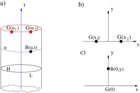
Figure 1: Periodic boundary conditions. a) The observables in the stationary state of a stochastic process $G(u_{1})$ and $G(u_{2})$ are attached to the rim of the half-cylinder. They are used when computing the space two-point function. $B(u,t)$ is an observable on the surface of the half-cylinder. It is used when computing space and time correlators. b) $G(x_{1})$ and $G(x_{2})$ are boundary fields in the half-plane. c) $G(0)$ is a boundary field at $x=0$, $B(0,y)$ is a bulk field at $x=0$ and $y$. The Hamiltonian $H$ at time $t$ (negative) acts on the circle of length $L$

In order to get the space correlation functions on the half-cylinder, one uses the fact that they are known in the half-plane and that one can make a conformal transformation from the half-plane to the half cylinder. We denote by $z=x+iy$ ($y\geq 0$) and $w=t+iu$ ($t\leq 0$) the complex coordinates, and take Neumann boundary conditions at $y=0$. This choice corresponds to $\langle 0|^{s}=(1,1,\ldots,1)$ in the stochastic process. The correlation function of two boundary fields $G(x_{1})$ and $G(x_{2})$ (they are situated at $y=0$ and shown in Fig. 1b) is known from conformal field theory [8]:

$$\langle 0|G(x_{1})G(x_{2})|0\rangle=|x_{2}-x_{1}|^{-2\Delta}.$$ (2.1)

Here $\Delta$ is the scalling dimension of the boundary field $G$. The Kac table provides the following possible values for a $c=0$ theory:

$$\Delta=\frac{(3r-2s)^{2}-1}{24},$$ (2.2)

where $r$ and $s$ are nonnegative integers ($\Delta=0,1/8,1/3,5/8,1,35/24,\ldots$).

The transformation

$$w=\frac{L}{2\pi}\ln\left(\frac{1+iz}{1-iz}\right)$$ (2.3)

takes the half-plane to the half-cylinder and the two-point correlation function on the top of the half-cylinder follows:

$$\langle 0|^{s}G(u_{1})G(u_{2})|0\rangle=\left(\frac{dx_{1}}{du_{1}}\right)^{\Delta}\left(\frac{dx_{2}}{du_{2}}\right)^{\Delta}\langle 0|G(x_{1})G(x_{2})|0\rangle.$$

Taking $L\to\infty$ with $u_{1}$ and $u_{2}$ fixed, as well $|u_{2}-u_{1}|$ large, one obtains:

$$\langle 0|^{s}G(u_{1})G(u_{2})|0\rangle=|u_{2}-u_{1}|^{-2\Delta}.$$ (2.4)

This is an interesting result: although the stochastic process takes place in a system with periodic boundary conditions, one doesn’t have left and right movers. One has only one Virasoro algebra and not two as it is the case for periodic boundary conditions in the equilibrium problem.

The one-point function vanishes for large $L$. The large $L$ behavior is given by the scaling dimension of the boundary operator. Assuming that on the half-line,

$$\langle 0|^{s}G(x)|0\rangle=C,$$ (2.5)

where $C$ is a constant and making the mapping (2.3) one obtains, for large $L$, the one-point function on the rim of the cylinder:

$$G_{L}(u)\sim~{}L^{-\Delta}.$$ (2.6)

In Sec. 4 and  5 we are going to make repeated use of Eq. (2.6).

If one is interested in time correlation functions $\langle 0|^{s}G(0)B(0,t)|0\rangle$ (for simplicity both observables have $u=0$), one looks again at the half-plane (see Fig. 1c) taking $x=0$ (i. e. $G(x=0)$) and $B(x=0,y)$. Like before, $G$ is a boundary field and $B$ is a bulk field. We have to keep in mind that the limit $y\to 0$ is singular (the bulk field $B$ doesn’t go smoothly to a boundary field). One has [4]:

$$\langle 0|G(0)B(0,y)|0\rangle=y^{-x_{B}-\Delta},$$ (2.7)

where $x_{B}$ is the conformal dimension of the bulk field $B$. We perform again the conformal transformation from the half-plane to the half-cylinder and get:

$$\langle 0|^{s}G(u=0)B(u=0,t)|0\rangle=|t|^{-x_{B}-\Delta}.$$ (2.8)

In order to derive (2.8) we have taken $L\to\infty$ with $t$ fixed. The expression (2.7) generalizes in a simple way when $G$ and $B$ have different space coordinates, say $u_{1}$ and $u_{2}$.

b) Open boundaries.

If the stochastic process has open boundaries, the problem is slightly more complicated. The system is not defined on a half-cylinder but on a half-strip of width $L$ (see Fig. 2). We consider the case of only one observable in the stationary state and study the finite-size scaling effects on the one-point function $G_{L}(u)$ ($u=0,\ldots,L$). The two-point correlation function implies the knowledge of model dependent correlations in the half-plane.

Figure 2: Open system. a) the strip $w=t+iu$ on which the stochastic process takes place. The stationary state is at $t=0$. The boundary operator $G(u)$ is attached on the top of the strip. b) The half-plane $z=x+iy$ in which the conformal field theory is used. $C(-1)$ and $C(1)$ are boundary changing fields applied at $x=-1$ and $x=1$.

In order to get the expression of the one-point function, one consider the half-plane with the $y=0$ axis divided by the points $A$ ($x=-1$) and $C$ ($x=1$). Between $A$ and $C$ ( $-1<x<1$) one takes Neumann boundary conditions. For $x<-1$ and $x>1$, we don’t need to specify the boundary conditions except that they are the same. We attach to the points $A$ and $C$, boundary changing fields [4] $C(-1)$ and $C(1)$. In order to find $G(x)$, we consider the vacuum expectation of the 3-point function given by conformal filed theory:

$$\langle 0|\phi_{a}(x_{1})\phi_{b}(x_{2})\phi_{c}(x_{3})|0\rangle>=\frac{C_{abc}}{(x_{2}-x_{1})^{\Delta_{a}+\Delta_{b}-\Delta_{c}}(x_{2}-x_{3})^{\Delta_{b}+\Delta_{c}-\Delta_{a}}(x_{3}-x_{1})^{\Delta_{a}+\Delta_{c}-\Delta_{b}}},$$ (2.9)

where $\Delta_{a}$, $\Delta_{b}$ and $\Delta_{c}$ are the scaling dimensions of $\phi_{a}$, $\phi_{b}$ and $\phi_{c}$. Taking $\Delta_{a}=\Delta_{c}$, $\Delta_{b}=\Delta$ and using (2.9) one gets:

$$\langle 0|C(-1)G(x)C(1)|0\rangle\sim(1-x^{2})^{-\Delta}.$$ (2.10)

We use the Schwarz-Christoffel mapping which takes the half-plane to the strip: $z=-\cosh(\pi w/L)$ ($z=x+iy$, $w=t+iu$) and obtain

$$G_{L}(u)=\left(\frac{dz}{dw}\right)^{\Delta}\langle 0|C(-1)G(x)C(1)|0\rangle\sim\left(\frac{L}{\pi}\sin(\pi u/L)\right)^{-\Delta}.$$ (2.11)

This result is interesting since there is a theorem [8] which says that in equilibrium, the one-point function vanishes unless one has a left-hand mover with a scaling dimension equal to the one of the right-hand mover therefore one has:

$$G_{L}(u)_{\mbox{\scriptsize{eq}}}\sim\left(\frac{L}{\pi}\sin(\pi u/L)\right)^{-2\Delta}.$$ (2.12)

Notice the exponent $\Delta$ in (2.11) as compared to $2\Delta$ in (2.12).

For not symmetric boundary conditions, similar to the equilibrium problem [9], Eq. (2.11) generalizes as follows:

$$G_{L}(u)\sim F(\cos(\pi u/L))\left(\frac{L}{\pi}\sin(\pi u/L)\right)^{-\Delta}.$$ (2.13)

The time dependence of the one-point function can also be easily obtained but for the application we have in mind (2.11) is enough.

We have to stress that these results were obtained assuming that in the stochastic process one uses observables which are local. As we are going to see in the next sections, to find local observables is not an easy task.

In Sec. 4 and  5 we compare the expressions (2.4), (2.6), (2.11) and (2.13) with the correlation functions seen in the Raise and Peel model. This model is described in the next section.

3 The Raise and Peel model

There are plenty of papers [5] describing this model, written after the discovery by Razumov and Stroganov [10], that its stationary state has magic combinatorial properties. We give here a short survey of the model which should allow the reader to follow the results presented in Secs. 4 and  5.

One considers a Hamiltonian given by the expression:

$$H=\sum_{i=1}^{M}(1-e_{i}),$$ (3.1)

where $M=L-1$, for the open system and $M=L$ for the periodic one. $e_{i}(i=1,\ldots,M)$ are the generators of the Temperley-Lieb algebra for the open system and of the periodic Temperley Lieb algebra for the periodic one. They verify the relations

$$e_{i}^{2}=(q+1/q)e_{i}$$ (3.2)

$$e_{i}e_{i\pm 1}e_{i}=e_{i}$$ (3.3)

$$e_{i}e_{k}=e_{k}e_{i},\quad|i-k|>1.$$ (3.4)

In the case of the periodic algebra, which is infinite dimensional, another relation is needed in order to get a finite dimensional quotient [11]. We skip it here. The algebras have a representation in terms of Pauli matrices and one obtains a Hamiltonian given by an XXZ quantum chain with $L$ sites having the $U_{q}(sl(2))$ symmetry for the open system. In this case the Hamiltonian is not Hermitian. In the periodic case, one gets the XXZ chain with twisted boundary conditions where the twist depends on $q$. $H$ is Hermitian in this case. The spectra of the Hamiltonians are known and for $|q|=1$, they are gapless. Taking $q=\exp(i\pi/3)$ the ground-state eigenvalue is zero for any value of $L$, and the other energy levels are positive and therefore one can look for stochastic base.

We consider the case $L$ even only. There are three equivalent stochastic base, each one useful for different purposes. The simplest one is given by Dyck paths. They are defined in terms of heights $\{h_{i}\}$ obeying the restricted solid-on-solid rules:

$$h_{i+1}-h_{i}=\pm 1,\;i=0,1,\ldots,L,$$ (3.5)

with $h_{0}=h_{L}=0$ for the open system and $h_{i}=h_{L+i}$ for the periodic one. In Fig. 3 we show the six configurations in the periodic case $L=4$. There are $L!/\{(L/2+1)([L/2]!)^{2}\}$ configurations for the open system and $L!/[(L/2)!]^{2}$ for the periodic case.

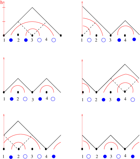
Figure 3: The three stochastic base, Dyck paths, particle-vacancy and link patterns base for $L=4$. There are 6 possible profiles. In the particle-vacancy representation the particles are full dots and the vacancies empty dots. The corresponding link patterns representation are also shown.

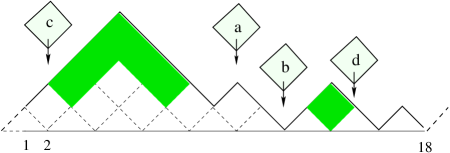
Figure 4: Example of a configuration with four peaks and three contact points in the periodic Raise ans Peel model with $L=18$ sites. Depending on the position where the tilted tiles reach the interface, several distinct processes occur (see the text).

In the stochastic basis of Dyck paths the time evolution of the system can be visualized in the following way. A Dyck path can be seen as separating droplets of tilted tiles from a rarefied gas of tilted tiles (see Figure 4). The Dyck path changes its shape as a result of hits from the tiles of the gas according to the following rules:

In a time interval $\Delta t$, with probability $p_{i}=\Delta t/L$ a given site $i$, with height $h_{i}$ is reached by a tilted tile of the gas phase (see Fig. 4). Several movements are possible depending on the local slop $s_{i}=(h_{i+1}-h_{i})/2$ at the site:

i) $s_{i}=0$ and $h_{i}>h_{i-1}$.

The tile hits a local peak (case $a$ in Fig. 4) and it is reflected leaving the profile unchanged.

ii) $s_{i}=0$ and $h_{i}<h_{i-1}$.

The tile hits a local minimum (case $b$ in Fig. 4). The tile is absorved ($h_{i}\to h_{i}+2$).

iii) $s_{i}=1$.

The tile is reflected after triggering the desorption of a layer of tiles from the segment $h_{j}>h_{i}=h_{i+b}$, $j=i+1,\ldots,i+b-1$, i. e., $h_{j}\to h_{j}-2$ for $j=i+1,\ldots,i+b-1$ (case $c$ of Fig. 4). The desorbed layer contains $b-1$ tiles (always an odd number).

iv) $s_{i}=-1$.

The tile is reflected after triggering the desorption of a layer of tiles from the segment $h_{j}>h_{i}=h_{i+b}$, $j=i-b+1,\ldots,i-1$, i. e., $h_{j}\to h_{j}-2$ for $j=i-b+1,\ldots,i-1$ (case $d$ of Fig. 4).

These evolution rules take place in discrete time by choosing, for example, $\Delta t=1$ as usual in Monte Carlo simulations or in continuum time by taking $\Delta t=1/L\to 0$.

There is a one-to-one correspondence among the Dyck path configurations $\{h_{i}\}$ and the configurations $\{n_{i}\}$ of particles ($n_{i}=1$) and vacancies ($n_{i}=0$) attached to the links of the $L$ sites chain, namely,

$$n_{i}=\frac{h_{i+1}-h_{i}+1}{2},\quad(i=1,2,\ldots,L),\quad h_{L+1}=h_{1}.$$ (3.6)

For illustration the configurations for the $L=4$ sites system are also shown in Fig. 3. This correspondence imply that the number of particles and vacancies are equal to $L/2$. The time-evolution rules of this half-filling chain of particles are directly obtained from the corresponding rules for the heights we defined (see [7]). In this particle language we have a nonlocal asymmetric exclusion model where the particles either jump to the next-nearest neighbor position (corresponding to adsorption) at its left, or jump nonlocally to a site position on its right (corresponding to desorption).

We have just described the second stochastic basis, the particle-vacancy one. This representation as well as the Dyck path one correspond to the $S^{z}=0$ sector of the XXZ quantum chain. It can be enlarged to the full $2^{L}$ dimensional representation as shown in [7]. A third stochastic basis is the link patterns basis. It is obtained from the Dyck paths basis in the following way. For each height $h_{i}$ ($i=1,...,L$) one draws $h_{i}$ noncrossing arches which end up at different sites. When all sites $i$ are considered, arches end up at all sites. In Fig. 4 we illustrate the correspondence between the two base for $L=4$. The dynamics of the system in the link patterns basis follows the one in the Dyck path basis.

4 Connection with the loop gas and the SOS models

The stationary state of the Raise and Peel model with periodic boundary conditions in the link patterns basis can be understood in terms of a $Q=1$ loop gas model [4] on a half-cylinder (see Figs. 1 and 5). We have in mind the discussion in Sec. 2 about the applications of conformal invariance. The rim of the cylinder corresponds to the stationary state. We give here a short summary of this connection (see [4, 3] for more details).

One takes a lattice on the half-cylinder and consider only the configurations of self and mutually avoiding fully packed loops. The configurations of the loop model are either closed loops (they don’t reach the rim of the cylinder at $t=0$) shown in black, or arches which start and end on the rim, colored in Fig. 5. All arches have a fugacity equal to 1. The probability to have a certain configuration in the stationary state of the stochastic model is proportional to the partition function on the half-cylinder with the given configuration as a boundary condition. This observation is relevant since one can map the loop model into a solid-on-solid (SOS) model on the lattice. In the continuum space and time limit, the latter model is described by a free bosonic conformal field theory on the rim of the half-cylinder [4]. The model is parameterized by the parameters $e_{0}$ equal to 1/3 and the coupling $g=2/3$ in our case. If we denote by $G(u)$ the boundary bosonic field (with Neumann boundary conditions on the boundary) the correlator is

$$<G(u)G(u^{\prime})>=-3/2\ln|u-u^{\prime}|^{2}.$$ (4.1)

We define the vertex operators $V_{\pm}(u)=\exp(\pm i(e_{1}+e_{0}/2)G(u))$. The use of the new parameter $e_{1}$ will be clear soon. The correlator of two vertex operators is

$$<V_{+}(u)V_{-}(u^{\prime})>\sim|u-u^{\prime}|^{-2\Delta},$$ (4.2)

with

$$\Delta=(36e_{1}^{2}-1)/24.$$ (4.3)

We can now use Eqs. (2.5), (2.6), (4.3) and get for large values of $L$:

$$<V_{\pm}>=A(e_{1})L^{-\Delta}.$$ (4.4)

$A(e_{1})$ is a function which has to be determined. Consider now the generating function

$$M(w)=\sum_{\{h_{i}\}}P_{\{h_{i}\}}w^{h_{i}},$$ (4.5)

where $P_{\{h_{i}\}}$ is the probability to have a height $h_{i}$ (Dyck path representation) at the site $i$. The site independence of $M(w)$ is a consequence of the translational invariance of the stochastic model. This corresponds to $h_{i}$ arches crossing the link $i$ between the sites $i$ and $i+1$ (see Fig. 6)

It is important to note that following [4, 3] we can get the identity

$$<V_{\pm}>=M(w),$$ (4.6)

where

$$w=2\cos(\pi e_{1})/\sqrt{3}.$$ (4.7)

In the next section we will discuss the implications of the relation

$$M(w)=A(w)L^{-\Delta(w)}$$ (4.8)

for the Raise and Peel model. Although the relation (4.8) might have been derived somewhere else, we have checked it using computer simulations. In Fig. 7 we show the values of the generating function $M(w)$ as a function of the lattice size $L$ for 3 values of $w$:

$$w_{1}=\frac{1}{\sqrt{3}},\quad\Delta=\frac{1}{8}=0.125;\quad w_{2}=\sqrt{\frac{2}{3}},\quad\Delta=0.05208333...;$$

$$w_{3}=\frac{\sqrt{3}}{2},\quad\Delta=0.037720222...\quad.$$ (4.9)

The fits are done using Eq. (4.8) and they are excellent. From the fits we obtain

$$A(1/\sqrt{3})=0.850;\quad A(\sqrt{2}/3)=0.936;\quad A(\sqrt{3}/2)=0.954.$$ (4.10)

The value $A(1)=1$ is a consequence of the normalization of the probability function $P_{\{h_{i}\}}$ in Eq. (4.5). For completeness we also give the value

$$A(0)=2\frac{\Gamma(5/6)}{3\sqrt{\pi}}=0.424...$$ (4.11)

This value will be derived in the next section.

We consider now the two-point function (4.2) and look at the lattice realization of it. We take a segment $(i,j)$ on the rim of the half-cylinder and consider the generating function:

$$M^{\prime}(u;w)=\sum_{h_{i},h_{j}}w^{h_{i}+h_{j}}P(h_{i},h_{j}),$$ (4.12)

where $P(h_{i},h_{j})$ is the probability to have the heights $h_{i}$ and $h_{j}$, and $u=j-i$. If one looks at the computer simulations one discovers that the function $M^{\prime}(u;w)$ is not independent on $L$ for large lattice sizes. To find the proper definition of the generating function, it is better to use the arches language. If one considers the segment (see Fig. 6), there are two sorts of arches. The first one are those which start at sites smaller than $i$ and end up at sites larger than $j$ or starts and ends at the sites between $i$ and $j$. The second one are the arches which start inside and end outside the segment between $i$ and $j$. We call them non-crossing arches (NCA). If we disregard the first kind of arches, in the calculation in the new generating function $M(w)$ one finds, in agreement with (4.2)

$$M(u;w)=B(w)u^{-2\Delta(w)},$$ (4.13)

with $\Delta$ given by (4.3). This implies $B(1)=1$, again from the normalization of the probability function. The same calculation can be done in terms of Dyck paths. If we define $h_{\mbox{\scriptsize{min}}}$ as the minimum height in the segment $(i,j)$

$$h_{\mbox{\scriptsize{min}}}=\mbox{Min}\{h_{i},h_{i+1},\ldots,h_{j}\},$$ (4.14)

we recover the generating function $M(u;w)$:

$$M(u;w)=\sum_{h_{i},h_{j}}w^{(h_{i}-h_{\mbox{\scriptsize{min}}})+(h_{j}-h_{\mbox{\scriptsize{min}}})}P(h_{i},h_{j}).$$ (4.15)

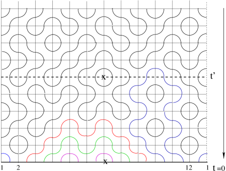
Figure 5: A configuration of self and mutually avoiding fully packed loop model with $L=12$ sites in the periodic spacial direction (horizontal). The time direction is the vertical direction. The closed arches in the bulk (black loops) as well the closed arches (colored arches) that starts and close at the surface (time $t$) have a Boltzmann weight 1.

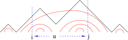
Figure 6: A configuration with the segment ($i,j$). $h_{i}=2$, $h_{j}=3$. One arch enters the segment at $i$ and leaves it at $j$.

There is an important conclusion coming from this exercise. The boundary two-point function of the bosonic field theory has a nonlocal lattice realization. Indeed, if we fix the segment, the end-points of the segment alone don’t fix the paths, one has to look at the whole segment and find the value of $h_{\mbox{\scriptsize{min}}}$ for each configuration. In Sec. 5 we discuss the implications of the connection between the generic function $M(u;w)$ and the two-point function (4.2).

The results described up to now can be generalized. Take again the segment $(i,j)$ and denote $u=j-i$. Consider the generic function:

$$M(u;w_{1},w_{2})=\sum_{\{h_{i}\}}w_{1}^{h_{i}-h_{\mbox{\scriptsize{min}}}}w_{2}^{h_{j}-h_{\mbox{\scriptsize{min}}}}P(h_{i},h_{j}).$$ (4.16)

we conjecture that in the large $L$ limit, we have

$$M(u;w_{1},w_{2})=\frac{C(w_{1},w_{2})}{u^{\Delta(w_{1})+\Delta(w_{2})}},$$ (4.17)

where $C(1,1)=1$. Obviously we recover (4.13) if $w_{1}=w_{2}=w.$ Numerics suggest that $C(w_{1},w_{2})=A(w_{1})A(w_{2})$, where $A(w)$ is defined by (4.8).

The conjecture (4.17) was checked using Monte Carlo simulations for several pairs of values $(w_{1},w_{2})$. In Figs. 8 and  9 we show the results for the pairs $(1/\sqrt{3},\sqrt{2/3}))$ respectively $(\sqrt{2/3},\sqrt{3/4})$.

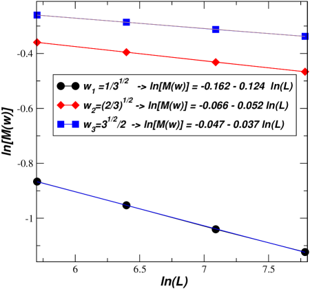
Figure 7: The one-point function (4.8) as a function of the lattice size L for the three values of $w$ given in (4). From the fits on can read the values of $\Delta$ and $A(w)$.

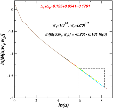
Figure 8: The two-point function $M(u;w_{1},w_{2})$ defined in (4.17) as a function of $u$ for the values $w_{1}=1/\sqrt{3}$ and $w_{2}=\sqrt{2/3}$. The predicted result follows from (4) and is given in the figure. The lattice sizes are $L=300,600,1200,2400,4800$ and $9600$. The fitting was done for the largest lattice and in the region of the dashed box shown in the figure.

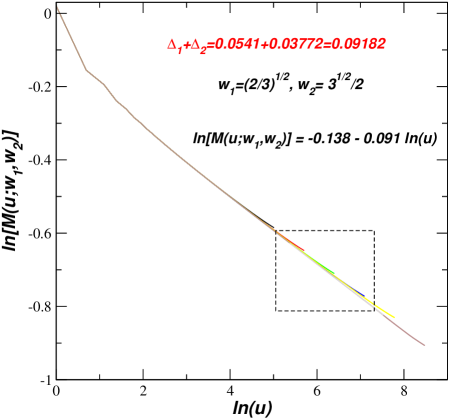
Figure 9: Same as Fig. 8 for the two-point function one $M(u;w_{1},w_{2})$ defined in (4.17) for the values $w_{1}=\sqrt{2/3}$ and $w_{2}=\sqrt{3}/2$

.

We have taken several values of $L$: 300, 600, 1200, 2400, 4800 and 9600. One can see that the data are independent on $L$. Moreover, the $u$ dependence is correctly given by (4.17) when using the exponents (4).

We are not aware of any field theoretical derivation of the two-fugacity generating function so our results stay as a conjecture.

5 Correlation functions in the Raise and Peel model and conformal invariance

In Sec. 2 we have given the predictions on conformal field theory for the correlators of stochastic models. These predictions were made for local boundary operators. We have described in Sec. 3 the Raise and Peel model which is conformal invariant but in the stochastic base, the Hamiltonian acts in a nonlocal way therefore the task is to identify local operators in the stochastic base. In Sec. 4 we have shown that the vertex operators of the bosonic boundary field theory are indeed local but that the lattice model from which they can be derived is nonlocal. In this section we are going to clarify the problem and make clearer the connection between the previous sections. We discuss separately the periodic system and the open one

a) Periodic boundary conditions.

We consider first the particles-vacancy stochastic basis. A natural local variable is the particle density. One expects (2.4) to be valid and this is indeed the case. In Fig. 10 we show the density-density correlator $<\eta(0)\eta(u)>$ obtained from Monte Carlo simulations for different lattice sizes ($\eta(u)$ is the density of particles minus 1/2). There is no lattice dependence and one obtains an exponent $\Delta=0.983$ which within errors is equal to 1, one of the exponent given by (2.2). This exponent is the one one expects on dimensional grounds and will also be obtained in the open system.

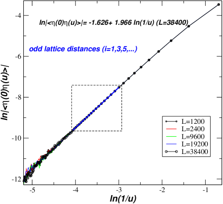
Figure 10: Particle densitity correlator as a function of $u$ Correlation of density of particles for the periodic RPM. The data are for the lattice sizes $L=1200,2400,9600,19200$ and $38400$. The plot is in a log-log scale considering only the odd lattice distances.

Another local observable is the current density in the stationary state. It was shown in [12] that its expression for large $L$ is:

$$J(L)=\frac{3}{4L}.$$ (5.1)

One would expect therefore on the two-current correlator $<J(0)J(u)>$ an exponent $2\Delta=2$. Monte Carlo simulations (see Fig. 11) give an exponent equal to 1.028 which is close to 1 and not to 2. We have no explanation for this observation.

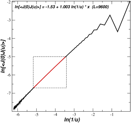
Figure 11: Current density correlator as a function of $u$ for the periodic RPM. The data are for $L=9600$

There is no obvious connection between the bosonic boundary field theory and the density of particles as well the current density observables.

We consider now the Dyck paths stochastic basis. A natural local observable is the density $R(L)$ of contact points ($h_{i}=0$) (see Fig. 4). There is an exact result for this quantity. It is based on a conjecture by de Gier [13] for the number of clusters for any $L$. A cluster is a segment between two consecutive contact points. This conjecture was verified by Monte Carlo simulations. The expression of the density for large $L$ is;

$$R(L)=\frac{2}{3}\sqrt{\pi}\Gamma(5/6)/L^{1/3}.$$ (5.2)

This gives an exponent $\Delta=1/3$, again given by (2.2). The same result is obtained using (4.3) and (4.7) with $w=0$.

The definition of the two-contact-point correlation has to be considered with care. If one uses the SOS prescription discussed in Sec. 4, one has to use Eq. i(4.2) for $w=0$ and get from (4.3) and (4.7) $\Delta=1/3$. We have checked this prediction using Monte Carlo simulations. This implies that one has to take into account not only the configurations in which $h_{i}=h_{j}=0$ ($j-i=u$) but also all the configurations in which $h_{i}=h_{j}=h_{\mbox{\scriptsize{min}}}$. Those are the NCA configurations. It turns out that if we take into account only the configurations with contact points ($h_{i}=h_{j}=0$) the two-point function vanishes in the large $L$ limit but it does so in a neat, unexplained. way:

$$M^{\prime}_{L}(u,0)\sim(Lu)^{-1/3}.$$ (5.3)

The physical interpretation of (5.3) is the following one. The conditional probability to have a contact point at the distance $u$ from a given contact point (that happens with probability $L^{-1/3}$) decreases like $u^{-1/3}$.

Before closing this section we give some results which can be obtained using the generating functions $M(w)$ (Eq. (4.8)), $M(u;w)$ (Eq. (4.13)) and $M(u;w_{1},w_{2})$ (Eq. (4.17)) defined in Sec. 4. One obtains in this way properties of the Dyck paths configurations in the large $L$ limit.

From the one-point vertex $M(w)$ (4.8) one obtains

$$<h^{n}>=\left.\left(w\frac{d}{dw}\right)^{n}M(w)\right|_{w=1},$$ (5.4)

$$P(h=n)=<\delta_{h,n}>=\frac{1}{n!}\left.\frac{d^{n}}{dw^{n}}M(z)\right|_{w=0}.$$ (5.5)

It is easy to derive the leading behavior:

$$<h>=\frac{\sqrt{3}}{2\pi}\ln{L},$$ (5.6)

$$\sigma_{h}^{2}=<h^{2}>-<h>^{2}=\frac{2\sqrt{3}\pi-9}{\pi^{2}}\ln{L},$$ (5.7)

and

$$P(h=0)=A(0)L^{-1/3},\quad P(h=1)=A(0)\frac{3\sqrt{3}}{4\pi}\frac{\ln{L}}{L^{1/3}},$$

$$P(h=2)=A(0)\left(\frac{27}{32\pi^{2}}\frac{(\ln L)^{2}}{L^{1/3}}-\frac{9}{8\pi^{2}}\frac{\ln{L}}{L^{1/3}}\right),$$ (5.8)

with $A(0)$ given by (4.11).

From $M(u;w_{1},w_{2})$ (Eq. (4.16)) we get the leading behavior:

$$<h_{i}-h_{\mbox{\scriptsize{min}}}>=\left.\frac{\partial}{\partial w_{1}}M(u;w_{1},w_{2})\right|_{w_{1}=w_{2}=1}=\frac{\sqrt{3}}{2\pi}\ln{u}.$$ (5.9)

Notice that in the large $u$ limit $<h-h_{\mbox{\scriptsize{min}}}>$ coincides with (5.6). This implies that the average number of arches crossing a link is equal to the average number of arches entering the segment of length $u$ from one side or the other. The double of this quantity is called valence bond bipartite entanglement entropy (see e.g. in [14, 3]).

An interesting quantity is the average probability to have a height $(h_{i}-h_{\mbox{\scriptsize{min}}})=m$ at the site $i$ and a height $(h_{j}-h_{\mbox{\scriptsize{min}}})=n$ at the site $j$. Using (4.16) and (4.17) one finds the leading behavior:

$$P_{m,n}(u)\sim|\ln(u)^{m+n}|u^{-2/3}.$$ (5.10)

b) Open boundary conditions.

We consider first symmetric boundary conditions and a stochastic basis with particles and vacancies in an open segment of length $L$ ($L$ even). Let $u$ be the distance from one of the boundaries and $\rho$ the density of particles from which one has subtracted 1/2 (the average value). Using Monte Carlo simulations [15] we have found

$$\rho=C\frac{\pi}{L\sin(\pi u/L)},$$ (5.11)

where $C$ is a constant. Using (2.11) we find $\Delta=1$ in agreement with the result obtained in the periodic boundary case.

We next consider the density of contact points $R_{L}(u)$. An exact result is known in this case [5, 15]:

$$R_{L}(u)=C_{1}\left(\frac{\pi}{L\sin(\pi u/L)}\right)^{1/3},$$ (5.12)

where $C_{1}=-\sqrt{3}\Gamma(-1/6)/(6(\pi)^{5/6})=0.7531...$ . Comparing with (2.11) one finds $\Delta=1/3$ in agreement with what was obtained in the periodic case.

The case of nonsymmetric boundaries was studied in Ref. [15]. The one-boundary Temperley Lieb algebra was used adding a boundary generator to the Hamiltonian (3.1) and the function $F(\cos(\pi u/L))$ in Eq. (2.13) was identified for both the densities of particles and of contact points.

6 Conclusions

We think that in this paper we have clarified the consequences of conformal invariance in stochastic processes. The main ingredient is the realization that if one looks at space dependent correlators one deals not with bulk operators but with Neumann boundary operators. Since there are no left and right movers in this case, the critical exponents are half of what one would expect for a periodic system. Space and time correlators imply that one has to consider also bulk operators in the vicinity of the boundary. One conclusion is that one shouldn’t expect the standard relativistic space-time dependence $x^{2}+t^{2}$ of the correlators.

This picture was verified in the Raise and Peel model which has a simple, albeit nonlocal dynamics which allows Monte Carlo simulations on large lattices. We have checked in this way the predictions of conformal invariance when analytical results were not available.

Because of the nonlocal dynamics, the identification of local operators in the stochastic base for which conformal field theory makes predictions, is not an obvious task. This identification is dependent on which basis was chosen.

In the particle-vacancy basis, we have checked that the particle density is a bona fide local operator with scaling dimension $\Delta=1$. The current density operator on the other hand has a correlator with an unexplained behavior. In the Dyck paths basis, one can use the mapping of the model onto the SOS model which in continuum space and time is described by a bosonic free field theory. Using boundary vertex operators with a known behavior, one can go backwards and identify the local operators in the lattice model.

Looking at Dyck paths, the density of contact (zero height) points look as a natural candidate for a local operator. Examining the behavior of the one-point function, it looks that this is the case. One finds a scaling dimension $\Delta=1/3$. Looking however at the two-contact point correlator, we discover that it vanishes at large values of $L$. The $L$ and $u$ (the distance between the two contact points) dependence is simple, it involves again the exponent 1/3, but the expression of the correlator remains a puzzle. The way to solve the problem comes from the bosonic field theory. If one takes the segment between the two points where the correlator is computed, one sees that for each configuration one has a minimum height $h_{\mbox{\scriptsize{min}}}$. If one subtracts from each height $h_{\mbox{\scriptsize{min}}}$ one gets new contact points for which $h-h_{\mbox{\scriptsize{min}}}=0$. If one takes into account now all the configurations having contact points including also of those of the new kind at the end of the segment one finds a non-vanishing correlator with the proper critical exponent. This is the NCA (non-crossing arches correlation).

Let us observe that from all the possible scaling dimensions (2.3) available for a $c=0$ theory, we found only two of them: 1/3 and 1.

As a byproduct of our research, we made the conjecture (4.12) on the average probability to have two different subtracted ($h_{\mbox{\scriptsize{min}}}$ is taken away) heights at the end of a given segment. This conjecture was checked in Monte Carlo simulations.

As the reader might have observed, we have not touched on the space and time correlators. To our knowledge, exact results are not known and computer simulations on very large lattices have large finite-sizes corrections depending on the initial conditions. We plan to look in the future at this problem.

Before closing the paper, we would like to observe that with the exception of several versions of the Raise and Peel model, no other models with conformal invariance and a simple dynamics are known. This is an invitation for more research in this field

7 Acknowledgments

VR would like to thank David Mukamel for his kind invitation to the Department of Physics of Complex Systems at the Weizmann Institute where part of this work was done. and FCA to FAPESP and CNPq (Brazilian agencies) for financial support.

References

- [1] Halpin-Healy T, Kazumasa A and Takeuchi K A, 2015 arXiv:1505.01910 and references therein
- [2] Alcaraz F C and Rittenberg V, 2007 Phys. Rev. E 75 051110
- [3] Jacobsen J L and Saleur H, 2008 Phys. Rev. Lett. 100 087205
- [4] Kostov I K, Ponsot B,and Serban D, 2004 Nucl. Phys. B 683 309-362; Kazakov V and Kostov I, 1992 Nucl. Phys. B386 520-557
- [5] de Gier J, Nienhuis B, Pearce P A and Rittenberg V, 2004 J. Stat. Phys. 114 1-35
- [6] Alcaraz F C and Rittenberg V, 2012 J. Stat. Mech. JSTAT P05022; Alcaraz F C and Rittenberg V, 2010 J. Stat. Mech. JSTAT P12032
- [7] Alcaraz F C and Rittenberg V, 2013 J. Stat. Mech. JSTAT P09010
- [8] Cardy J, 2008 on Lectures given at les Houches arXiv:0807.3472
- [9] Burkhardt T W and Hue T, 1991 Phys. Rev. Lett. 66 895
- [10] Razumov A V, Stroganov Yu G, 2001 J. Phys. A 34 5335
- [11] Levy D, 1991 Phys. Rev. Lett. 67 1971, Martin P and Saleur H, 1993 Comm. Math. Phys. 158 155; 1993 Lett. Math. Phys. 30 189
- [12] Pyatov P , private communication
- [13] de Gier J, 2005 Discr. Math. 298 365-388
- [14] Alet F, Capponi S, Laflorencie N and Mambrini M, 2007 Phys. Rev. Lett. 99 117204; Chhajlany R W , Tomczak P and Wojcik A, 2007 Phys. Rev. Lett. 99 167204
- [15] Alcaraz F C, Pyatov P and Rittenberg V, 2008 J. Stat. Mech. JSTAT P01006