Communication shapes sensory response in multicellular networks

Abstract

Collective sensing by interacting cells is observed in a variety of biological systems, and yet a quantitative understanding of how sensory information is collectively encoded is lacking. Here we investigate the ATP-induced calcium dynamics of monolayers of fibroblast cells that communicate via gap junctions. Combining experiments and stochastic modeling, we find that increasing the ATP stimulus increases the propensity for calcium oscillations despite large cell-to-cell variability. The model further predicts that the oscillation propensity increases not only with the stimulus, but also with the cell density due to increased communication. Experiments confirm this prediction, showing that cell density modulates the collective sensory response. We further implicate cell-cell communication by coculturing the fibroblasts with cancer cells, which we show act as “defects” in the communication network, thereby reducing the oscillation propensity. These results suggest that multicellular networks sit at a point in parameter space where cell-cell communication has a significant effect on the sensory response, allowing cells to simultaneously respond to a sensory input and to the presence of neighbors.

I Significance Statement

Cells routinely sense and respond to their environment, and they also communicate with each other. Communication is therefore thought to play a crucial role in sensing, but exactly how this occurs remains poorly understood. We study a population of fibroblast cells that responds to a chemical stimulus (ATP) and communicates by molecule exchange. Combining experiments and mathematical modeling, we find that cells exhibit calcium oscillations not only in response to the ATP stimulus, but also in response to an increase in cell density. To confirm that the density dependence is a result of increased cell-cell communication, we combine the fibroblasts with cancer cells, which we show have weakened communication properties. The oscillations indeed decrease with the fraction of cancer cells. Our results show that when cells are together, their sensory responses reflect not just the stimulus level, but also the degree of communication within the population.

II Introduction

Decoding the cellular response to environmental perturbations, such as chemosensing, photosensing, and mechanosensing has been of central importance in our understanding of living systems. Up to date, most studies of cellular sensation and response have focused on single isolated cells or population averages. An emerging picture from these studies is the set of design principles governing cellular signaling pathways: these pathways are organized into an intertwined, often redundant network, and the network architecture is closely related with the robustness of cellular information processing Lauffenburger2000 ; Darnell2000 . On the other hand, many examples suggest that collective sensing by many interacting cells may provide another dimension for the cells to process environmental cues Barritt1994 . Quorum sensing in bacterial colonies Bassler2001 and cyclic adenosine monophosphate (cAMP) signaling in Dictyostelium discoideum populations Sawai2010 generate dramatic group behaviors in response to environmental stimuli. Various types of collective sensing have also been observed for higher level multicellular organisms, such as in the olfaction of insects Vosshall2007 and mammals Smear2011 , the glucose response in the pancreatic islet benninger2008gap , and the visual processing of animal retinal ganglion cells Bialek2006 ; Chichilnisky2011 . These examples suggest a fundamental need to revisit cellular information processing in the context of multicellular sensation and responses, since even weak cell-to-cell interaction may have strong impacts on the states of multicellular network dynamics Bialek2006 . In particular, we seek to examine how the sensory response of cells in a population differs from that of isolated cells, and whether we can tune between these two extremes by controlling the degree of cell-cell communication.

Previously, we have described the spatial-temporal dynamics of collective chemosensing of a mammalian cell model system Sun2012 ; Sun2013b . In this model system, high density mouse fibroblast cells (NIH 3T3) form a monolayer that allows nearest-neighbor communications through gap junctions Gilula1996 . When extracellular ATP is delivered to the cell monolayer, P2 receptors on the cell membrane trigger release of the second messenger IP3 (Inositol 1,4,5-trisphosphate) Irvine1989 . IP3 molecules, when binding to their receptors at the membrane of endoplasmic reticulum (ER), open ion channels to allow influx of Ca²⁺ from the ER to the cytoplasm. The fast increase in cytosolic calcium concentration is followed by a slow decrease when Ca²⁺ are pumped back to the ER Snyderc1990 . This simple picture, however, is complicated by the nonlinear feedback between Ca²⁺ and ion channel opening probability, which leads to rich dynamic behaviors such as cytosolic calcium oscillations Putney2011 . In the situation of collective ATP sensing, we have found that gap junction communications dominate intercellular interactions Sun2012 . Furthermore, these short-range interactions propagate and turn the cell monolayer into a percolating network Sun2013b . These characteristics make the system ideal for studying how sensory responses are modulated by extensive communication in multicellular networks.

Here we use this model system to examine how cell-cell communication affects collective chemosensing. Combining experiments with stochastic modeling, we find that cells robustly encode the ATP stimulus strength in terms of their propensity for calcium oscillations, despite significant cell-to-cell variability. The model further predicts that the oscillation propensity depends not only on the stimulus, but also on the density of cells, and that denser monolayers have narrower distributions of oscillation frequencies. We confirm both predictions experimentally. To verify that the mechanism behind the density dependence is the modulation of cell-cell communication, we introduce cancer cells (MDA-MB-231) into the fibroblast cell monolayer. As we show, MDA-MB-231 cells act as “defects” in the multicellular network, as they have distinct calcium dynamics when compared with the fibroblasts due to reduced gap junction communication Kanno1966 ; Laird2006 ; Jiang2014 . We find that the oscillation propensity of the fibroblasts decreases as the fraction of cancer cells increases, confirming that the sensory response is directly affected by the cell-cell communication. Our findings indicate that cells’ collective response to a sensory stimulus is distinct from their individual responses, and that in this case the response simultaneously encodes both the stimulus strength and the degree of communication within the population.

III Results

In order to study the sensory responses of a multicellular network, we use single channel microfluidic devices and deliver ATP solutions to monolayers of fibroblast (NIH 3T3) cells (see Appendix A). The stimuli solutions of ATP concentrations varying from 0 $\mu$M to 200 $\mu$M are pumped though the channel at rate of 50 $\mu$l/min, ensuring minimal flow perturbation to the cells and fast delivery of ATP across the field of view. During this time we record the calcium dynamics of each individual cell loaded with fluorescent calcium indicator (Fluo-4, Life Technologies) at 4 frames/sec (Hamamatsu Flash 2.8, Hamamatsu). Our analysis uses 400 seconds of data from each recording selected such that ATP arrival is at approximately 50 seconds.

We modulate the degree of communication in two ways. First, we vary the cell density. Smaller cell densities correspond to larger cell-to-cell distances, which we expect to reduce the probability of forming gap junctions. Second, we coculture the fibroblasts with breast cancer (MDA-MB-231) cells in the flow channel (see Appendix A). As we later show, MDA-MB-231 cells have reduced communication properties and therefore act as defects in the multicellular network. To distinguish the two cell types, MDA-MB-231 cells are pre-labeled with red fluorescent dye (Cell Tracker Red CMTPX, Life Technologies). Varying cell density and the fraction of cancer cells allows us to control the architecture of the multicellular network over a wide range.

Figure 1A shows the composite image of a high-density cell monolayer with cocultured fibroblast and cancer cells. In this example, MDA-MB-231 cells make up a fraction $F_{C}=$ 15% of the total population which has a total cell density of $\rho_{T}=$ 2500 cells/mm². At this density, each cell has an average of 6 nearest neighbors from which extensive gap junction communication is expected. After identifying cell centers from the composite image (see Appendix A), we compute the time-dependent average fluorescent intensity near the center of each cell which represents the instantaneous intracellular calcium concentration at the single cell level.

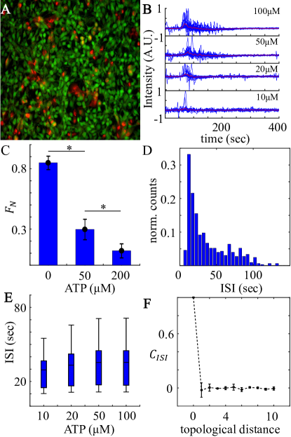
Figure 1: Calcium dynamics of cell monolayer in response to extracellular ATP. (A) Composite image showing the multicellular network of cocultured fibroblast (NIH 3T3) and breast cancer cells (MDA-MB-231). Red: MDA-MB-231. Green: fluorescent calcium signal for all cells (MDA-MB-231 and NIH 3T3). (B) Normalized fluorescence intensity profiles of one typical experiment for each ATP concentration tested. Blue: randomly selected single cell calcium responses. Red: average intensity profiles of all cells in each experiment. All time series begin approximately 50 seconds before arrival of ATP stimuli. Intensity profiles of individual cells have been rescaled to $[-1,\,1]$. (C) Fraction of non-oscillating cells $F_{N}$ as a function of ATP concentration at fixed cell density ($\rho_{T}=1200\pm 200$ cells/mm²) and cancer cell fraction ($15\%\pm 6\%$). Error bars: SEM for $n\geq 4$. (D) ISI event counts normalized by number of cells for only NIH 3T3 cells. (E) Average experimentally-measured ISI values of NIH 3T3 cells at varying ATP concentrations at fixed cell density ($\rho_{T}=1200\pm 200$ cells/mm²) and cancer fraction ($F_{C}=15\%\pm 6\%$). (F) ISI cross-correlation as a function of topological distance. Data from experiments with 50 $\mu$M ATP, at fixed cell density ($\rho_{T}=1400\pm 400$ cells/mm²) and cancer fraction ($F_{C}=20\%\pm 5\%$). Error bars show standard deviation from five experiments.

III.1 Collective response to ATP stimuli

Typical responses of cells to excitation by ATP are shown in Fig. 1B. We see that, on average, higher concentrations of ATP trigger larger increases in calcium levels. Cell-to-cell variations are significant; for example, response times as well as subsequent calcium dynamics of individual cells vary dramatically amongst cells in the same multicellular network. In many cells, the initial calcium increase is followed by transient calcium oscillations. We quantify the oscillation propensity by computing the fraction of non-oscillating cells $F_{N}$ using a peak-finding algorithm (see Appendix B). We see in Fig. 1C that higher concentrations of ATP cause a larger percentage of cells to oscillate, and thus a smaller $F_{N}$.

The period of the oscillation is characterized by the inter-spike interval (ISI), which has been proposed to dynamically encode information about the stimuli Tang1995 ; Falcke2014 . To investigate the characteristics of ISI in the context collective chemosensing, we systematically study the statistics of the ISI from 30,000 cells. Figure 1D shows the histogram (event counts) of ISI values, normalized by the number of cells, of a typical experiment where the ATP concentration is 50 $\mu$M. We see that the distribution is broad, which underscores the high degree of cell-to-cell variability in the responses. Figure 1E summarizes the distribution at each ATP concentration using a box-and-whisker plot. We see that there is no significant dependence of the ISI on the ATP concentration. This is at odds with a familiar property of calcium oscillations, termed frequency encoding, in which the oscillation frequency (or ISI) depends on the strength of the stimulus Putney2011 ; Tang1995 ; Woods1986 ; Meyer1991 . However, we will see in the next section that the lack of a dependence here is likely due to the high degree of cell-to-cell variability.

Finally, we characterize the spatial correlations of the ISI within the monolayer by computing the cross-correlation function $C_{ISI}(d)$ as a function of topological distance $d$ between cells. In particular, for each experiment, we first identify all oscillatory cells and compute the average ISI $T_{i}$ for each cell $i$. We then define $\delta T_{i}=T_{i}-\langle T_{i}\rangle$, and $C_{ISI}(d)=\langle\delta T_{i}\delta T_{j}\rangle_{D_{ij}=d}/\langle\delta T_{i}^{2}\rangle$, where $D_{ij}$ is the topological distance between cells $i$ and $j$. Figure 1F shows that $C_{ISI}(d)$ falls off immediately for $d>0$. This is surprising, since the cells experience identical ATP stimuli, and one might hypothesize that communication between cells would result in the ISI values for nearby cells being correlated. However, as described next, evidence from mathematical modeling suggests that this correlation is removed by the cell-to-cell variability.

III.2 Stochastic modeling of the collective response

To obtain a mechanistic understanding of the experimental observations, we turn to mathematical modeling. We develop a stochastic model of collective calcium signaling based on the work of Tang and Othmer Tang1995 ; Othmer1993 . Their model captures the ATP-induced release of IP3, the IP3-triggered opening of calcium channels in the ER, and the nonlinear dependence of the opening probability on the calcium concentration, as schematically illustrated in Fig. 2A. The model neglects more complex features of calcium signaling observed in some cell types, such as upstream IP3 oscillations Stryer1988 ; Hofer2006 and spatial correlations among channels Champeil1999 ; Falcke2004 . The model predicts that at a critical ATP concentration, the calcium dynamics transition from non-oscillating to oscillating. However, it was previously only analyzed deterministically for a single cell Tang1995 ; Othmer1993 . Therefore we extend it to include both intrinsic noise and cell-cell communication via calcium exchange (see Appendix C). We also explicitly include the dynamics of IP3, which has a constant degradation rate and a production rate $\alpha$ that we take as proportional to the ATP concentration. We simulate the dynamics using the Gillespie algorithm Gillespie1977 , and we vary the density $\rho_{T}$ of cells on a square grid, which modulates the degree of communication.

Figure 2B shows the dependence of $F_{N}$ on $\alpha$, where $\alpha$ is the model analog of the experimentally controlled ATP concentration. Consistent with the experimental findings in Fig. 1C, we see that $F_{N}$ decreases with $\alpha$. In the model, the decrease is due to the fact that intrinsic noise broadens the transition from the non-oscillating to the oscillating regime. Thus, instead of a sharp transition from $F_{N}=1$ to $F_{N}=0$ as predicted deterministically, the transition occurs gradually over the range of $\alpha$ shown in Fig. 2B. Figure 2C shows the dependence of the ISI on $\alpha$ in the model (see the green box plots). We see that the ISI decreases with $\alpha$, which is expected since frequency encoding is a component of the Tang-Othmer model Tang1995 ; Othmer1993 . Yet, this property is not consistent with the experimental observation in Fig. 1E, where the ISI shows no clear dependence on ATP concentration. Further, Fig. 2D shows the dependence of the correlation function $C_{ISI}$ on the topological distance $d$ in the model (see the green curve). We see that $C_{ISI}$ decreases gradually with $d$, indicating nonzero spatial correlations in the ISI. This feature is again inconsistent with the experimental findings seen in Fig. 1F.

Motivated by the high level of cell-to-cell variability evident in Figs. 1B and 1D, we hypothesize that cell-to-cell variability is responsible for these discrepancies between the model and the experiments. Indeed, inspecting the ISI histogram from the model reveals a very narrow distribution of ISI values, as seen in Fig. 2E (green bars), which is in contrast to the broad distribution observed experimentally in Fig. 1D. To incorporate cell-to-cell variability, we allow the model parameters to vary from cell to cell. Lacking information about the susceptibility of particular parameters to variation, we allow all model parameters to vary by the same maximum fold change (i.e., parameters are sampled uniform randomly in log space). The maximum fold change $F$ is found by equating the variance of the resulting ISI distribution with that from the experiments, which yields the value $F=2$ (see Appendix C). As seen in Fig. 2E (blue bars), the resulting ISI distribution is consistent with that observed in Fig. 2D, both in width and in shape.

We see in Fig. 2C (blue box plots) that including cell-to-cell variability in the model severely weakens the decrease of the ISI with $\bar{\alpha}$, therefore agreeing with the experimental results shown in Fig. 1E (with variability, $\bar{\alpha}$ is defined as the mean of the $\alpha$ values sampled for each cell). We also see in Fig. 2D (blue curve) that variability removes the correlations $C_{ISI}$ for $d>0$, which is consistent with the immediate fall-off observed experimentally in Fig. 1F. Importantly, even with variability, the decrease of $F_{N}$ with $\alpha$ seen in Fig. 2B persists, as demonstrated in Fig. 2F. This decrease remains consistent with the experimental observation in Fig. 1C. Indeed, variability significantly broadens the range of $\bar{\alpha}$ values over which the transition occurs, as expected (compare Fig. 2F to Fig. 2B), which is consistent with the broad range over which the transition occurs experimentally (Fig. 1C).

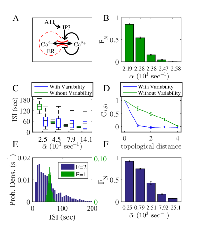
Figure 2: Model development and validation. (A) Schematic of the model. ATP stimulates IP3 release at rate $\alpha$, and IP3 acts jointly with Ca²⁺ to open calcium channels (positive feedback), while further Ca²⁺ binding closes channels (negative feedback). Communication is modeled via diffusion of Ca²⁺ between adjacent cells. (B) Fraction of non-oscillating cells $F_{N}$ as a function of ATP-induced IP3 production rate $\alpha$. (C) Interspike interval (ISI) decreases with $\bar{\alpha}$ (green). The decrease is severely weakened by cell-to-cell variability (blue). (D) ISI cross-correlation as a function of topological distance $d$ (green). Cell-to-cell variability removes correlations for $d>0$. (E) Distribution of ISI values (green). Cell-to-cell variability significantly broadens distribution (blue). (F) $F_{N}$ versus $\bar{\alpha}$ with cell-to-cell variability. In B and F, error bars are SEM for $n=5$ subsamples.

III.3 Effects of communication on the sensory response

Having validated the model, we now use it to make predictions about the effect of cell-cell communication on collective calcium dynamics. Communication in the model is controlled by cell density, with higher density leading to more cell-to-cell contacts and thus a higher degree of communication. Therefore we first investigate the dependence of the oscillation propensity on the cell density. Fig. 3A shows $F_{N}$ as a function of both cell density $\rho_{T}$ and the ATP-induced IP3 production rate $\bar{\alpha}$. We see that the fraction of non-oscillating cells transitions from $F_{N}=1$ to $F_{N}=0$ as a function of $\bar{\alpha}$ and that there is also a dependence of $F_{N}$ on $\rho_{T}$. Not only has intrinsic noise and cell-to-cell variability broadened the $F_{N}$ transition as a function of $\bar{\alpha}$, but evidently cell-cell communication has introduced a dependence of the transition on cell density. The result is that at low $\bar{\alpha}$, $F_{N}$ is everywhere large and is independent of cell density (Fig. 3B and left box in Fig. 3A). However, at intermediate $\bar{\alpha}$, $F_{N}$ is a decreasing function of cell density (Fig. 3C and right box in Fig. 3A). In this regime, increasing the degree of communication causes more cells to exhibit oscillatory calcium dynamics (thus decreasing $F_{N}$), even with a fixed sensory stimulus $\bar{\alpha}$. At large $\bar{\alpha}$ (beyond the range of Fig. 3A), we have checked that the non-oscillating fraction is driven to low values as expected, and the density dependence of $F_{N}$ diminishes.

The prediction in Fig. 3C is striking because it implies that cell-cell communication causes more cells to oscillate, even while cell-to-cell variability causes their ISI values to be spatially uncorrelated (Fig. 2D). Therefore, we wondered whether communication would have an effect on the width of the ISI distribution in this regime. The width, or more generally the amount of uncertainty contained in the ISI distribution, is characterized by the entropy. For a continuous variable $x$, the entropy becomes the differential entropy, defined as $H_{ISI}=-\int\rho(x)\log\rho(x)dx$, where $\rho(x)$ is the probability density. As seen in Fig. 3E, the entropy of the ISI distribution increases with $F_{N}$. This indicates that as communication decreases the non-oscillating fraction, it also narrows the distribution of ISI values.

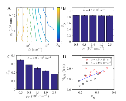
Figure 3: Model predictions. (A) Fraction of non-oscillating cells $F_{N}$ as a function of cell density $\rho_{T}$ and ATP-induced IP3 production rate $\bar{\alpha}$. Left and right boxes correspond to B and C, respectively. (B) At small $\bar{\alpha}$, $F_{N}$ is large and density-independent. (C) At intermediate $\bar{\alpha}$, $F_{N}$ decreases with density. In B-D, error bars are SEM for $n=5$ subsamples. (D) Entropy of ISI distribution $H_{ISI}$ increases with $F_{N}$.

We now test these predictions in our experimental system. To test our predictions about how the non-oscillating fraction of cells should depend on cell density, we measure $F_{N}$ as a function of $\rho_{T}$ for various ATP concentrations. We see in Fig. 4A that with no ATP, $F_{N}$ is large at both low and high densities, and there is no statistically significant correlation between $F_{N}$ and $\rho_{T}$. Then, we see in Fig. 4B that at intermediate ATP concentrations ($10$$-$$100$ $\mu$M), $F_{N}$ significantly decreases with $\rho_{T}$ (see Appendix B for pairwise statistical comparison of particular density values). Finally, we see in Fig. 4C that at large ATP concentration (200 $\mu$M), $F_{N}$ is small at both low and high densities, and again there is no statistically significant correlation between $F_{N}$ and $\rho_{T}$. These results confirm the predictions in Fig. 3.

To test the prediction that the entropy of the ISI distribution increases with the non-oscillating fraction of cells, we measure $H_{ISI}$ as function of $F_{N}$. As seen in Fig. 4D, $H_{ISI}$ increases with $F_{N}$, consistent with the prediction in Fig. 3D. This implies that cell density regulates the spectrum of the ISI response. In particular, it suggests that increasing the degree of cell-cell communication narrows the distribution of ISI, making the ISI values less variable across the cell population. We have also checked that the entropy of the distribution of cross-correlation values for nearest neighbors’ entire calcium trajectories $C_{NN}$ Sun2012 ; Sun2013b decreases as a function of cell density (see Appendix D). $C_{NN}$ is not only a statistical characterization of the collective cellular dynamics, but also may provide robust channel for cellular information encoding Bialek2006 ; Meister1996 ; Meister2003 . Together, these results imply that cell-cell communication has a significant effect on the collective sensory response. This finding is especially striking given the strong effects of cell-to-cell variability (Fig. 1E and F). We conclude that the effects of communication observed here persist in spite of extensive cell-to-cell variability.

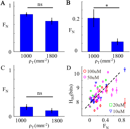
Figure 4: Experimental tests of model predictions. (A) Fraction of non-oscillating NIH 3T3 cells $F_{N}$ as a function of cell density $\rho_{T}$ when stimulated by 0 $\mu$M ATP. Error bars: SEM for $n>4$. ns, not significant. (B) As in A, but with intermediate concentrations $10$$-$$100$ $\mu$M ATP. (C) As in A, but with 200 $\mu$M ATP. In A-C, the cancer cell fraction is fixed at $F_{C}=15\%\pm 6\%$. (D) $F_{N}$ is positively correlated with the differential entropy of inter-spike intervals $H_{ISI}$. Error bars represent standard deviation of 1000 bootstrap resampled results, see Appendix D for more details.

III.4 Effect of cancer cell “defects”

We have seen that increasing cell density increases the propensity of cells to oscillate in response to an ATP stimulus. This behavior is consistent with our model, which predicts that the mechanism is through increased cell-cell communication. However, it could be in the experiments that increasing the cell density introduces other effects beyond increased gap-junction communication, such as mechanical coupling between cells or coupling to the substrate Janmey2011 . To modulate the communication directly, we vary the fraction $F_{C}$ of cancer cells with which the fibroblasts are cocultured, while keeping the density of all cells fixed. Since cancer cells are known to have reduced gap junction communication Kanno1966 ; Laird2006 ; Jiang2014 , we expect the fraction of non-oscillating cells $F_{N}$ to have the opposite dependence on $F_{C}$ that it does on cell density (Fig. 4B).

First we investigate whether MDA-MB-231 cells indeed have reduced communication in our system. Figure 5A shows several examples of single-cell calcium dynamics for NIH 3T3 and MDA-MB-231 cells in a typical experiment. We see that both cell types exhibit immediate increases in cytosolic calcium levels at the arrival of ATP, but cancer cells typically show long relaxation times while fibroblast cells tend more often to exhibit oscillations after stimulation. These qualitative features are maintained across all ATP concentrations. Figure 5B shows a comparison of the intercellular diffusion coefficients in the two cell types, obtained from a fluorescence recovery after photobleaching (FRAP) analysis Didelon2008 (see Appendix A). We see in Fig. 5B that gap junction-mediated diffusion between MDA-MB-231 cells is significantly weaker than between NIH 3T3 cells, consistent with previous reports Kanno1966 ; Laird2006 ; Jiang2014 . It is therefore evident that MDA-MB-231 cells can be treated as communication defects in the co-cultured multicellular network. Indeed, Fig. 5C shows the spatial distribution of these defects in the monolayer. In Fig. 5C, the mean ISI for each cell is shown in color, with non-oscillating cells in black. We see that cancer cells, labeled by white circles, are more likely to be non-oscillating, which is consistent with the qualitative characteristics shown in Fig. 5A. We have further quantified the distinction between the two cells types in Appendix B, where we show using the distributions of ISI values that oscillatory events are at least five times less likely to occur for the MDA-MB-231 cells.

Having established that the presence of cancer cells reduces the degree of cell-cell communication in the monolayer, we now vary the fraction of cancer cells and measure the oscillation propensity of the remaining fibroblasts. Fig. 5D shows the non-oscillating fraction of fibroblasts $F_{N}$ (blue bars) as a function of the cancer cell fraction $F_{C}$ for a typical experiment at fixed cell density ($\rho_{T}=1200\pm 200$ cells/mm²). We see that $F_{N}$ significantly increases with $F_{C}$ (see Appendix B for pairwise statistical comparison of particular $F_{C}$ values). We also see that $F_{N}$ for all cells (both fibroblasts and cancer cells, red bars) significantly increases with $F_{C}$, and that, as expected, $F_{N}$ is larger for all cells than for just fibroblasts. These findings imply that reduced cell-cell communication decreases the propensity for calcium oscillations, which is consistent with the effects of varying cell density (Fig. 4B). Finally, we also investigate the effect of cancer cells on the entropy of the ISI distribution. As shown in Appendix B, $H_{ISI}$ is higher for cells that are surrounded by a large number of cancer cells, and lower for cells with pure fibroblast neighbors. In the latter case, $H_{ISI}$ also increases as the number of nearest neighbors decreases. These findings imply that reduced cell-cell communication increases the entropy of the ISI values, even at the local level of a cell’s microenvironment, which is consistent with the effects seen in Fig. 4D. Taken together, we conclude that the calcium dynamics of individual cells are strongly regulated by the degree of gap junction communication inside the cell monolayer.

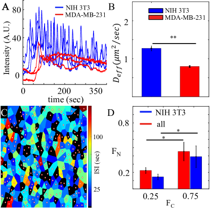
Figure 5: Effects of cancer cell “defects” on collective response. (A) Typical fluorescence intensity profiles showing the calcium dynamics on the single cell level, where basal level intensity has been subtracted. For each cell, basal level intensity is estimated by averaging 100 seconds of its fluorescent intensity before ATP arrival. (ATP concentration = $50$ $\mu$M, $\rho_{T}$ = 2400 cells/mm², $F_{C}$ = 12%). (B) Fluorescence recovery after photo bleaching (FRAP) experiments confirm that MDA-MB-231 cells have weaker gap junction communication compared with NIH 3T3 cells (error bars: SEM for $n>100$). See Appendix A for more details. (C) Spatial map of average ISI of each individual cell. ATP concentration is 50 $\mu$M. Black: non-oscillating cell. Circle: MDA-MB-231 cell. (D) When stimulated by an intermediate concentration of ATP ($10$$-$$100$ $\mu$M) the fraction of non-oscillating cells $F_{N}$ increases with increased cancer fraction $F_{C}$ at fixed total cell density ($\rho_{T}=1200\pm 200$ cells/ mm²). Blue: fraction of non-oscillating NIH 3T3 cells. Red: fraction of non-oscillating cells including both cell types.

IV Discussion

We have characterized the collective calcium dynamics of multicellular networks with varying degrees of cell-cell communication when they respond to extracellular ATP. These networks consist of cocultured fibroblast (NIH 3T3) and cancer (MDA-MB-231) cells. We have revealed their properties using a combination of controlled experiments and stochastic modeling. We have found that increasing the ATP stimulus increases the propensity for cells to exhibit calcium oscillations, which is expected at the single cell level. However, we have also found that increasing the cell density alone, while keeping the stimulus fixed, has a similar effect, revealing a purely collective component to the sensory response. Modeling suggests that this effect is due to an increased degree of molecular communication between cells. In line with this prediction, we have found that increasing the fraction of cancer cells in the monolayer reduces the oscillation propensity, as cancer cells act as defects in the communication network.

Typical physiological concentrations of extracellular ATP are tens of nM and larger schwiebert2003extracellular ; falzoni2013detecting ; trabanelli2012extracellular , but hundreds of $\mu$M has been associated with disease pellegatti2008increased . This suggests that healthy tissues in vivo are restricted to the regimes of Fig. 4A and B, and not C ($200$ $\mu$M). In the regime of Fig. 4A, the calcium dynamics encode the stimulus strength. In the regime of Fig. 4B, the calcium dynamics encode two pieces of information simultaneously: the stimulus strength and the cell density. One may wonder why a system would evolve to encode two pieces of information in the same quantity. It is tempting to speculate that there is a benefit to having the sensory response of the system be a function of the population density, as in quorum sensing Bassler2001 or so-called dynamical quorum sensing based on collective oscillations mehta2010approaching ; de2007dynamical ; taylor2009dynamical . The particular benefit of such a strategy for these cells is unclear. In a similar vein, one may wonder whether it is possible for cells to deconvolve the two pieces of information from the calcium signal using a downstream signaling network. Such “multiplexing” has been shown to be possible with simple biochemical networks deRonde2011 , although the ways in which dynamic information is stored in, and extracted from, cellular signals is a topic of ongoing research Cheong2011 ; Wollman2014 .

Our results suggest that the dependence of the calcium response on both sensory and collective parameters persists despite significant cell-to-cell variability. Indeed, we have found that certain measures are robust to variability, such as the oscillation propensity and the entropy of the ISI distribution, while others are not, such as spatial correlations in the ISI and its dependence on the ATP input (frequency encoding). This implies that traditional measures of information encoding in calcium dynamics, such as frequency encoding Putney2011 ; Tang1995 ; Hofer2006 ; Woods1986 ; Meyer1991 , may have to be rethought in contexts where cell-to-cell variability is pronounced. It is becoming increasingly understood that variability is common in cell populations, and recent examples suggest it may even be beneficial. For example, recent studies in a related system (NF-$\kappa$B oscillations in fibroblast populations) also found a large degree of cell-to-cell variability Tay2010 and demonstrated that this variability allows entrainment of the population to a wider range of inputs Tay2015 .

In our model, the transition from the non-oscillatory to the oscillatory regime occurs due to a saddle-node bifurcation, a critical point in parameter space where the number of dynamical fixed points changes (see Appendix C). This transition is broadened by intrinsic noise and cell-to-cell variability into a critical “region”, while cell-cell communication causes the oscillation propensity to depend on cell density within this region (Fig. 3A). Nonetheless, the underlying mechanism remains the critical dynamical transition. Our finding that this region is broad, and our suggestion that it may be of some functional use for the system, resonates with recent studies that have argued that biological systems are poised near critical points in their parameter space Mora2011 ; Krotov2014 ; Hidalgo2014 . However, the connection between dynamical criticality, as in our model, and criticality in many-body statistical systems, remains to be fully explored.

Gap junctional communications exist among many types of cells. Therefore, our results may have far-reaching implications for other biological model systems such as neuronal networks or cardiovascular systems. It will be interesting to explore the extent to which distinctions in the calcium dynamics in these systems originate from differences in their degrees of cell-cell communication.

V Materials and Methods

V.1 Fabrication of Microfluidic Device

See Appendix A for detailed device fabrication and characteristics.

V.2 Cell Culture and Sample Preparation

NIH 3T3 and MDA-MB-231 cells were cultured in standard growth mediums (Dulbecco’s modified Eagle medium (DMEM) supplemented with 10% bovine calf serum and1% penicillin and DMEM supplemented with 10% fetal bovine serum, 1% penicillin, and 1% non-essential amino acids respectively). To prepare samples, cells were detached from culture dishes using TrypLE Select (Life Technologies) and suspended in growth mediums before pipetted into the microfluidics devices and allowed to form monolayers. If MDA-MB-231 cells were the dominant species (a fraction greater than 50% of all cells), they were first allowed to attach the glass bottom of the microfluidics devices. Red fluorescent tag (CellTracker, Life Technologies) was then applied and subsequently washed with growth medium. Finally, NIH 3T3 cells were injected into the device so that the desired cell density ($\sim$1000 cells/mm²) was reached. If NIH 3T3 cells were the dominant species, they were allowed to attach the glass bottom of the microfluidics devices first. MDA-MB-231 cells already loaded with CellTracker were then injected into the devices to reach the desired cell density. After incubating the microfluidics devices containing cell monolayers overnight, fluorescent calcium indicator was applied (Fluo4, Life Technologies) making the samples ready for imaging.

V.3 Fluorescence Imaging and Image Analysis

Fluorescence was detected using a inverted microscope (Leica DMI 6000B) coupled with a Hamamatsu Flash 2.8 camera. Movies were taken at a frame rate of 4 frame/sec with a 20x oil immersion objective. Image analysis and data processing were performed in MATLAB. (Details in SI).

V.4 Stochastic model of collective calcium dynamics

We extend the model in Tang1995 ; Othmer1993 to include intrinsic noise and cell-cell communication. We simulate the ensuing calcium dynamics of cells of various densities on a 3-by-3 grid (and 7-by-7 grid for Fig. 2D) using the Gillespie algorithm Gillespie1977 with tau-leaping Gillespie2001 ; Rathinam2003 ; Cao2006 ; Cao2007 ). We include cell-to-cell variability by sampling all model parameters from distributions that are uniform in log space, which varies fold-change up to a maximal value. For further details, see Appendix C.

Appendix A Additional information of experimental setup

A.1 Fabrication and characteristics of microfluidic device

The organic elastomer polydimethylsiloxane (PDMS, Sylgard 184, Dow-Corning) used to create the microfluidic devices is comprised of a two part mixture - a base and curing agent - that is mixed in a 10:1 ratio, degassed, and poured over a stainless steel mold before curing at 65^∘C overnight. Once cured, the microfluidic devices are cut from the mold, inlet/outlet holes are punched, and the device is affixed to a No. 1.5 coverslip via corona treatment. Figures 6A-C provide schematics of the design of the device as well as inner dimensions of the flow chamber.

To characterize the stimuli profile in the flow chamber, we use fluorescein (Sigma Aldrich) to replace ATP as our probe and record the fluorescent intensity in the same flow condition as in the ATP sensing experiments. Figure 6D shows the normalized fluorescent intensity as a function of time from two devices. We estimate the time takes to fill the field of view with chemical stimuli is about 1 second.

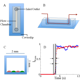
Figure 6: Design of the microfluidic device and stimuli arrival time (A) Top-view of microfluidic device showing glass slide, PDMS device, inlet/outlet, and connecting microfluidic chamber. (B) Side-view of microfluidic device indicating flow direction in red. (C) Cross-sectional view of device providing dimensions of flow layer and attached fibroblast (Green) and breast cancer (Red) cell monolayer. (D) Temporal profiles of chemical stimuli in the flow chamber evaluated using fluorescein. Two devices are tested (red and blue). Vertical lines correspond to arrival time and the times when half-maximum intensity reached.

A.2 Obtaining individual cell calcium dynamics

Application of CellTracker Red CMPTX (LifeTechnologies) to breast cancer cells and the calcium binding dye Alexa Fluo4 (LifeTechnologies) to both breast cancer cells and fibroblast cells within the microfluidic device allows for the differentiation of the two cell types. To do so, successive images are taken of the two fluorophores and first analyzed in ImageJ (imagej.nih.gov). Overlaying the two images generates a composite image that determines the network architecture, as is shown in Figure 1A of the main text. The centroids for each individual cell are manually determined and a dot is placed at the center of each cell as shown in Fig. 7. Using the dotted image as a mask, intensity is averaged over the $\sim$40 pixels comprising the dot for each cell and for all acquired frames in the experiment.

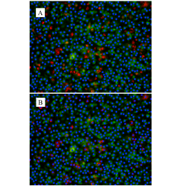
Figure 7: Determination of single cell centroids. (A) Composite image showing all cells (NIH 3T3 and MDA-MB-231, green), MDA-MB-231 (red), and manually determined centroids of NIH 3T3 cells (blue). (B) Composite image showing all cells (NIH 3T3 and MDA-MB-231, green), MDA-MB-231 (red), and manually determined centroids of all cells (NIH 3T3 and MDA-MB-231, blue).

A.3 Quantification of gap junctional intercellular communication

In order to quantify the gap junction communications for the two cell types we have used (NIH 3T3 and MDA-MB-231), we perform FRAP (fluorescent recovery after photobleaching) experiments to measure the effective diffusion coefficients in a cell monolayer for each cell type. (some experimental details, eg dye used frame rates etc). As shown in Fig. 8B, at each time point $t$, we represent the average concentration of fluorescent dye in the bleached area as $C_{i}(t)$ and non-bleached area as $C_{o}(t)$. The concentration of the dye is proportional to the recorded intensity as $C(t)=\alpha I(t)$, where $\alpha$ is a constant. We approximate the time evolution of $C_{o}(t)$ and $C_{i}(t)$ based on the following assumptions: (a) there is an overall bleaching rate $\beta$ while imaging, affecting both $C_{o}(t)$ and $C_{i}(t)$. (b) $C_{i}(t)$ get an influx due to a concentration gradient approximately proportionally to $D_{eff}\frac{C_{o}(t)-C_{i}(t)}{\frac{l}{2}}$, where $D_{eff}$ is the effective diffusion coefficient. (c) the cell monolayer has a uniform thickness of $h$. We have

$$\Delta C_{o}(t) = C_{o}(t+\Delta t)-C_{o}(t)\approx-\beta C_{o}(t)\Delta t$$ (1)

$$\Delta C_{i}(t) = C_{i}(t+\Delta t)-C_{i}(t)$$ (2)

$$\approx \frac{4lh}{hl^{2}}D_{eff}[C_{o}(t+\frac{\Delta t}{2})-C_{i}(t+\frac{\Delta t}{2})]\frac{1}{\frac{l}{2}}\Delta t-\beta C_{i}(t)\Delta t$$

The above equations can be simplified and we have

$$D_{eff}=\frac{l^{2}}{8\Delta t}\frac{\Delta I_{i}(t)-\Delta I_{o}(t)\frac{I_{i}(t)}{I_{o}(t)}}{I_{o}(t+\frac{\Delta t}{2})-I_{i}(t+\frac{\Delta t}{2})}$$ (3)

In our experiment, we take image at every 30 secs, therefore $\Delta t$ is set to be 1 minute. The recorded time series $I_{o}(t)$, $I_{o}(t)$ from all experiments are plugged into the above equation to obtain a distribution of the effective diffusion coefficient $D_{eff}$ as shown in Fig. 8D.

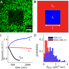
Figure 8: Estimation of the effective diffusion coefficients mediated by gap junctional communication in a cell monolayer. (A) Cell monolayer loaded with fluorescent dye (CellTracker Red CMPTX, LifeTechnologies) has been partially bleached. (B) The FRAP experiments can be quantified by the average intensity of the bleached area ($I_{i}$) and non-bleached area ($I_{o}$). (C) Normalized intensity profiles of a typical experiment. $I_{pb}$ is the intensity of the bleached area while being bleached. $I_{i}$ and $I_{o}$ are intensity profiles during recovery. (D) Histogram (normalized to probability) of the diffusion coefficients for NIH-3T3 cells and MDA-MB-231 cells.

Appendix B Additional information of Inter-Spike Interval (ISI) analysis

B.1 Inter-Spike Interval Determination

As calcium spike trains are unsuitable for Fourier analysis due to their varying amplitudes and irregular periods, the inter-spike interval (ISI) has been used as a suitable substitute for determining how the period of calcium oscillation affects information encoding within and amongst cells in the network. To determine the ISI’s from a single cell’s calcium dynamics $R(t)$, we first smooth the time series $R(t)$ to remove outlying data points Garcia2010 , to obtain $R_{s}(t)$. We then find all local peaks $\{t_{i}\}$ in $R_{s}(t)$ using the following criteria: a local peak must be higher than its neighboring valleys (local minimums) on both directions by a certain value, which we refer to as the sensitivity parameter; the first and last frames are excluded as peaks or valleys. Third, we obtain ISI’s $\{\delta t_{i}\}$ from the distances of peaks $\{\delta t_{i}=|t_{i+1}-t_{i}|\}$. Finally, to obtain the true ISI’s corresponding to calcium oscillations, we only keep $\{\delta t_{i}\}$ fall in the range of 5 seconds and 150 seconds. This final step excludes about 5% of ISI’s.

Figure 9A and 9B provide two examples of the peak finding algorithm’s ability to determine peak locations for a fibroblast cell calcium profile (A) and cancer cell calcium profile (B). The sensitivity parameter used for all experiments and in Figure 9A and 9B is $\frac{1}{4}$ the standard deviation of the normalized intensity $\sigma_{I}$ as determined empirically. Figure 9C and 9D show the algorithms diminished ability to determine peaks and to detect spurious peaks when the sensitivity parameter is set to $\sigma_{I}$ and $\frac{\sigma_{I}}{8}$ respectively.

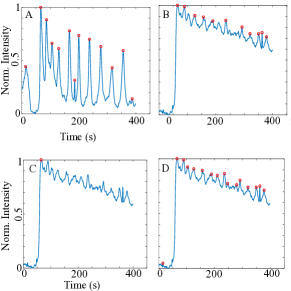
Figure 9: Intensity peak determination for single NIH 3T3 and MDA-MB-231 cell profiles. (A) Labeled peaks for a NIH 3T3 cell. Sensitivity parameter set to $\frac{1}{4}$ of the standard deviation of the time series. (B) Labeled peaks for a MDA-MB-231 cell. Sensitivity parameter set to $\frac{1}{4}$ of the standard deviation of the time series. (C) and (D) Same MDA-MB-231 intensity profile in (B) but with sensitivity parameter set to be the standard deviation and $\frac{1}{8}$ of the standard deviation of the time series respectively.

B.2 Spatial map of ISI in multicellular network

We have shown a map of ISI in Fig. 5C of the main text. To generate such a map, we first calculate the ISI’s corresponding to each individual cell as shown in the above. We then calculate the average ISI of each cell. Fig. 10 shows two more examples of the ISI spatial map. Figure 10A corresponding to a map from a experiment with 20$\mu$M ATP concentration and Fig. 10B corresponding to a 50$\mu$M ATP concentration. Black regions within the maps indicate cells that did not oscillate in the given experiment and a red circle indicates the location of a cancer cell. It is apparent from the figure that cancer cells are more likely to be non-oscillatory than fibroblast cells. This is also shown in Fig. 11, which shows ISI distributions of both cell types for a typical experiment.

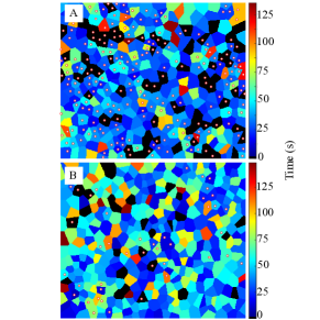
Figure 10: Spatial map of cell-average ISI of randomly selected experiment with (A) 20$\mu$M ATP. (B) 50$\mu$M ATP.

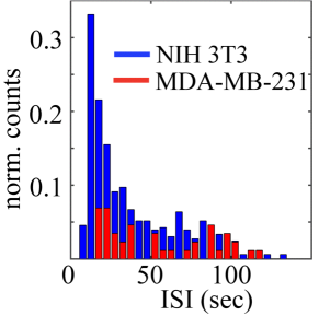
Figure 11: ISI characteristics of a typical experiment. ISI event counts normalized by number of cells. Blue: statistics of only NIH 3T3 cells, Red: statistics of only MDA-MB-231 cells.

B.3 Entropy of ISI distributions

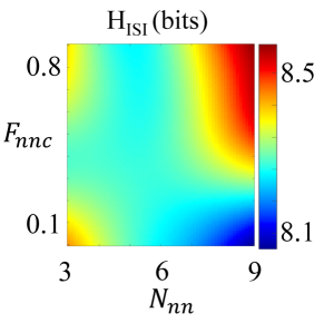
Figure 12: The spectrum of inter-spike intervals (ISI) as characterized by $H_{ISI}$ is regulated by the microenvironment of cells. For fixed ATP concentration (50 $\mu$M), calcium dynamics and the associated ISI of individual fibroblast cells are grouped based on the microenvironment of the cells. The microenvironment is characterized by the number of nearest neighbors ($N_{nn}$), among which a fraction of $F_{nnc}$ are cancer cells. The color map represents $H_{ISI}$ (in bits) at varying $N_{nn}$ and $F_{nnc}$, obtained by interpolating scattered data points with a Gaussian kernel.

Interestingly, the network architecture also regulates the spectrum of ISI. This can be demonstrated from the perspective of each individual cell’s microenvironment. We have grouped NIH 3T3 cells based on their number of nearest neighbors ($N_{nn}$), as well as the fraction of cancer cells in their $N_{nn}$ neighbors. For each group at a fixed ATP concentration (50 $\mu$M), we have computed the differential entropy of interspike intervals $H_{ISI}$. The differential entropy is computed using the k-nearest neighbor method, as described in Appendix D. As shown in Fig. 12, $H_{ISI}$ is higher for cells that are surrounded by a large number of cancer cells, and lower for cells with pure fibroblast neighbors. In the latter case, $H_{ISI}$ also increases as the number of nearest neighbors decreases. These results show that the spectrum of ISI is regulated by cell-cell communications both locally in the immediate microenvironment of a cell and globally throughout the whole defective multicellular network.

B.4 Statistics of $F_{N}$, the fraction of non-oscillating cells

As shown in Figs. 4 and 5 of the main text, the fraction of non-oscillating cells $F_{N}$ systematically depends on the network architecture. Fig. 13 shows pairwise statistical comparison of the results. The results are obtained by ANOVA followed with Fisher’s least significant difference procedure, implemented in MATLAB.

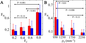
Figure 13: Statistical analysis of $F_{N}$ with varying cancer fractions (A) and cell densities (B). For both cases, the middle two groups do not show statistically significant differences. Therefore we have treated the middle two groups as a single group and performed ANOVA analysis. Notice that the blue bars, which represent non-oscillating fibroblast cells are not analyzed for p values.

Appendix C Theoretical Model

C.1 Deterministic Model

We model the dynamics of calcium release following Tang and Othmer Tang1995 . Their model is deterministic and valid for a single cell. First we describe the behavior of their model. Then we generalize it to include stochastic effects. Next, we generalize it further to include cell-cell communication. Finally, we add cell-to-cell variability. This procedure allows us to systematically explore the effects of stochasticity, communication, and variability on the calcium dynamics.

ATP triggers the production of IP₃ within a cell. IP₃ binds to receptors on the endoplasmic reticulum (ER). The ER is an internal store for calcium ions. When the receptors are active, they act as channels that allow passage of calcium between the ER and the cytoplasm of the cell. Receptor activation requires binding of both IP₃ and cytoplasmic calcium, such that calcium triggers its own release. However, an excess of calcium deactivates receptors, closing the channels. These positive and negative feedbacks, respectively, lead to oscillations and other rich dynamics.

The model of Tang and Othmer is based upon the following reactions,

$$C_{s}\xrightleftharpoons[\nu g_{0}]{g_{0}}C,\qquad C_{s}+R_{4}\xrightleftharpoons[\nu\gamma_{1}]{\gamma_{1}}C+R_{4},\qquad C\xrightarrow{\nu f(c)}C_{s},$$ (4)

$$R_{2}\xrightleftharpoons[k_{-1}]{k_{1}I}R_{3},\qquad R_{3}+C\xrightleftharpoons[k_{-2}]{\lambda_{2}}R_{4},\qquad R_{4}+C\xrightleftharpoons[k_{-3}]{\lambda_{3}}R_{5},\qquad$$ (5)

Eqn. 4 contains the reactions describing calcium transport between the ER and the cytoplasm, while Eqn. 5 contains the reactions describing the sequential (un)binding of molecules to receptors. In Eqn. 4, the first reaction describes leakage between the calcium in the ER ($C_{s}$) and calcium in the cytoplasm ($C$); $\nu$ is the ratio of the ER volume $V_{s}$ to the cytoplasm volume $V$. The second reaction describes transport of calcium through the receptor channels: receptors with both IP3 and calcium bound ($R_{4}$) are active channels. The last reaction describes the pumping of calcium from the cytoplasm to the ER; $f$ denotes the nonlinear pumping propensity. In Eqn. 5, the first reaction describes the binding of IP3 to bare receptors ($R_{2}$), creating the complex $R_{3}$; $I$ is the concentration of IP3, which is treated as a parameter in their model (we later generalize this feature, making $I$ a dynamic variable and its production rate $\alpha$ the control parameter, since this is more consistent with the experimental setup). The second reaction describes the subsequent binding of cytoplasmic calcium to the complex, which activates the complex ($R_{4}$). The last reaction describes the further binding of cytoplasmic calcium to another site on the complex, which deactivates the complex ($R_{5}$). Only receptors in the $R_{4}$ state serve as active channels.

The deterministic model describes the dynamics of the mean numbers of molecules. The dynamics follow directly from Eqns. 4 and 5. Introducing $n$ and $n_{s}$ as the numbers of calcium molecules in the cytoplasm and ER, respectively, and $m_{i}$ as the numbers of receptors in state $i\in\{2,3,4,5\}$, the means (denoted with an overbar) obey

$$\frac{d\bar{n}}{dt} = g_{0}\bar{n}_{s}-\nu g_{0}\bar{n}-\nu\pi_{1}\frac{\bar{n}^{2}}{\bar{n}^{2}+\pi_{2}^{2}}+\gamma_{1}\bar{n}_{s}\bar{m}_{4}-\nu\gamma_{1}\bar{n}\bar{m}_{4}$$

$$- \lambda_{2}\bar{m}_{3}\bar{n}+k_{-2}\bar{m}_{4}-\lambda_{3}\bar{m}_{4}\bar{n}+k_{-3}\bar{m}_{5},$$

$$\frac{d\bar{n}_{s}}{dt} = -g_{0}\bar{n}_{s}+\nu g_{0}\bar{n}+\nu\pi_{1}\frac{\bar{n}^{2}}{\bar{n}^{2}+\pi_{2}^{2}}-\gamma_{1}\bar{n}_{s}\bar{m}_{4}+\nu\gamma_{1}\bar{n}\bar{m}_{4},$$ (7)

$$\frac{d\bar{m}_{2}}{dt} = -k_{1}I\bar{m}_{2}+k_{-1}\bar{m}_{3},$$ (8)

$$\frac{d\bar{m}_{3}}{dt} = k_{1}I\bar{m}_{2}-k_{-1}\bar{m}_{3}-\lambda_{2}\bar{m}_{3}\bar{n}+k_{-2}\bar{m}_{4},$$ (9)

$$\frac{d\bar{m}_{4}}{dt} = \lambda_{2}\bar{m}_{3}\bar{n}-k_{-2}\bar{m}_{4}-\lambda_{3}\bar{m}_{4}\bar{n}+k_{-3}\bar{m}_{5},$$ (10)

$$\frac{d\bar{m}_{5}}{dt} = \lambda_{3}\bar{m}_{4}\bar{n}-k_{-3}\bar{m}_{5}.$$ (11)

The pumping propensity is a Hill function with coefficient $2$ and parameters $\pi_{1}$ and $\pi_{2}$.

Two quantities are conserved in the model: the total number of calcium molecules $n_{0}$ and the total number of receptors $m_{0}$,

$$n_{0} = n+n_{s}+m_{4}+2m_{5},$$ (12)

$$m_{0} = m_{2}+m_{3}+m_{4}+m_{5}.$$ (13)

The conservation relations reduce the number of dynamical equations from six to four. Specifically, we eliminate $n_{s}$ and $m_{4}$. Furthermore, we assume that the number of calcium molecules is much larger than the number of receptors, $n_{0}\gg m_{0}$. In this limit, introducing $c=(\bar{n}+\bar{m}_{4}+2\bar{m}_{5})/V$ as the concentration of calcium in the cytoplasm (both unbound and bound to receptors) and $x_{i}=m_{i}/m_{0}$ as the fraction of receptors in each state, Eqns. C.1-11 become

$$\frac{dc}{dt} = (1+\nu)(g_{0}+g_{1}x_{4})(c_{0}-c)-\nu p_{1}\frac{c^{2}}{c^{2}+p_{2}^{2}},$$ (14)

$$\frac{dx_{2}}{dt} = -k_{1}Ix_{2}+k_{-1}x_{3},$$ (15)

$$\frac{dx_{3}}{dt} = k_{1}Ix_{2}-k_{-1}x_{3}-k_{2}x_{3}c+k_{-2}x_{4},$$ (16)

$$\frac{dx_{5}}{dt} = k_{3}x_{4}c-k_{-3}x_{5},$$ (17)

where $x_{4}=1-x_{2}-x_{3}-x_{5}$, $g_{1}\equiv\gamma_{1}m_{0}$, $p_{1}\equiv\pi_{1}/V$, $p_{2}\equiv\pi_{2}/V$, $k_{2}\equiv\lambda_{2}V$, $k_{3}\equiv\lambda_{3}V$, and $c_{0}=n_{0}/(V+V_{s})$ is the average calcium concentration in both the cytoplasm and the ER. Eqns. 14-17 reproduce Eqn. 4 in Tang1995 . The parameter values used in Tang1995 , which we also use here, are given in Table 1.

Deterministic parameters	Stochastic parameters
	$V=200$ $\mu$m3
	$m_{0}=200$
$\nu=0.185$	$\nu=0.185$
$c_{0}=1.56$ $\mu$M	$n_{0}=(1+\nu)c_{0}V=2.2\times 10^{5}$
$g_{0}=0.025$ s-1	$g_{0}=0.025$ s-1
$g_{1}=36$ s-1	$\gamma_{1}=g_{1}/m_{0}=0.18$ s-1
$p_{1}=54$ $\mu$M$\cdot$s-1	$\pi_{1}=p_{1}V=6.5\times 10^{6}$ s-1
$p_{2}=0.03$ $\mu$M	$\pi_{2}=p_{2}V=3600$
$k_{1}=120$ $\mu$M${}^{-1}\cdot$s-1	$\lambda_{1}=k_{1}/V=0.001$ s-1
$k_{2}=150$ $\mu$M${}^{-1}\cdot$s-1	$\lambda_{2}=k_{2}/V=0.0013$ s-1
$k_{3}=0.18$ $\mu$M${}^{-1}\cdot$s-1	$\lambda_{3}=k_{3}/V=1.5\times 10^{-6}$ s-1
$k_{-1}=96$ s-1	$k_{-1}=96$ s-1
$k_{-2}=18$ s-1	$k_{-2}=18$ s-1
$k_{-3}=0.018$ s-1	$k_{-3}=0.018$ s-1
	$\alpha$ (varied)
	$\mu=0.058$ s-1
	$h=0.025$ s-1

Table 1: Parameters and their values. Deterministic values are taken from Tang and Othmer Tang1995 . Stochastic values follow from the deterministic values, given additional choices for the cytoplasmic volume $V$ and the total number of receptors $m_{0}$. These two parameters, as well as the additional parameters $\alpha$, $\mu$, and $h$, are estimated as described in the text.

Tang and Othmer recognize that the (un)binding of calcium to the deactivating site is slow compared to the other (un)binding reactions, $k_{3}\ll\{k_{1},k_{2}\}$ and $k_{-3}\ll\{k_{-1},k_{-2}\}$. This permits the quasi-steady-state approximations $dx_{2}/dt\approx 0$ and $dx_{3}/dt\approx 0$, which reduce Eqns. 14-17 to two equations. In dimensionless form they read

$$\epsilon\frac{dx}{d\tau} = \alpha_{1}(1-x)+\alpha_{2}(1-x)\frac{x(1-y)}{x+\beta_{1}[1+\beta_{0}(I)]}-\frac{x^{2}}{x^{2}+\alpha_{3}^{2}},$$ (18)

$$\frac{dy}{d\tau} = -y+\frac{\beta_{2}x^{2}(1-y)}{x+\beta_{1}[1+\beta_{0}(I)]},$$ (19)

where $x\equiv c/c_{0}$, $y\equiv x_{5}$, $\tau\equiv k_{-3}t$, $\epsilon\equiv k_{-3}c_{0}/\nu p_{1}$, $\alpha_{1}\equiv(1+\nu)c_{0}g_{0}/\nu p_{1}$, $\alpha_{2}\equiv(1+\nu)c_{0}g_{1}/\nu p_{1}$, $\alpha_{3}\equiv p_{2}/c_{0}$, $\beta_{0}(I)\equiv k_{-1}/k_{1}I$, $\beta_{1}\equiv k_{-2}/k_{2}c_{0}$, and $\beta_{2}\equiv k_{-3}c_{0}/k_{3}$.

Eqns. 18 and 19 exhibit four dynamic regimes. As shown in Fig. 14, the system can be (A) monostable, with low cytoplasmic calcium, (B) excitable, (C) oscillatory, or (D) monostable, with high cytoplasmic calcium. In the last regime (D), near the boundary, oscillations can also be supported for certain initial conditions. All four regimes are accessible by tuning the IP₃ concentration $I$ (Fig. 14E). Transitions between regimes occur at the critical concentrations $I^{*}_{1}$, $I^{*}_{2}$, and $I^{*}_{3}$. Of particular interest is the transition from the excitable to the oscillatory regime ($I^{*}_{2}$), since these are the dynamics exhibited by cells in the experiments: transient pulsing or sustained oscillations.

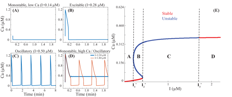
Figure 14: The deterministic model (Eqns. 18 and 19) exhibits four dynamic regimes: (A) monostable, with low cytoplasmic calcium, (B) excitable, (C) oscillatory, or (D) monostable, with high cytoplasmic calcium. In the last regime (D), near the boundary, oscillations can also be supported for certain initial conditions. (E) These regimes are accessible by tuning the IP₃ concentration $I$. The letters A-D in panel E correspond to the dynamics seen in panels A-D. The critical values $I_{1}^{*}$, $I_{2}^{*}$, and $I_{3}^{*}$ separating the regimes (dashed lines) are determined by changes in the number or stability of fixed points, which follow from a standard linear stability analysis. Parameters are listed in Table 1.

C.2 Stochastic Model

Stochastic dynamics are simulated using an adaptive tau-leaping method Gillespie2001 ; Rathinam2003 ; Cao2006 ; Cao2007 , which is a computationally-efficient approximation of the Gillespie algorithm Gillespie1977 . The simulation accounts for the facts that molecule numbers are integer-valued and that reactions fire at random, exponentially-distributed times. The reaction propensities follow directly from Eqns. 4-5, and have the same forms as the individual terms in Eqns. C.1-11 (without the overbars). The stochastic model parameters are related to the deterministic model parameters by the cytoplasmic volume $V$ and the total number of receptors $m_{0}$; see Table 1. Together these factors determine the noise in the system via the molecule numbers $n_{0}=(1+\nu)c_{0}V$ and $m_{0}$. Since relative fluctuations decrease with molecule number, large $n_{0}$ corresponds to low noise, while small $n_{0}$ corresponds to high noise. Typical trajectories are shown in Fig. 15.

We estimate the cell volume from the experiments. An upper bound is obtained from the measurements of the cell density $\rho$, since the cell area cannot be larger than $1/\rho$. The maximal density $\rho=2500$ mm^-2 gives the sharpest upper bound, for an area of $400$ $\mu$m², or a length scale of $20$ $\mu$m. Since this is an upper bound, we assume a length scale range of $10$$-$$20$ $\mu$m. For computational efficiency, we perform simulations assuming $10$ $\mu$m, and taking a monolayer width of $\sim$$2$ $\mu$m, this leads to a cell volume of $V=200$ $\mu$m³. Absent an experimental estimate for the number of receptors $m_{0}$, we take $m_{0}=200$.

In the stochastic model, we no longer treat $I$ (the concentration of IP3) as a parameter; instead, we treat the number of IP3 molecules as a stochastic variable. The control parameter is then the production rate of IP3, $\alpha$, which is assumed to be proportional to the ATP concentration in the experiments. IP3 is degraded at a rate $\mu$, meaning that the stochastic reactions simulated are Eqns. 4-5, with the first reaction of Eqn. 5 replaced with

$$I\xrightleftharpoons[\alpha]{\mu}\varnothing,\qquad R_{2}+I\xrightleftharpoons[k_{-1}]{k_{1}}R_{3}.$$ (20)

The degradation rate of IP3 has been measured to be $\mu=0.058$ s^-1 Wang1995 , and we vary $\alpha$ in the range $\sim$$10^{3}$$-$$10^{4}$ s^-1 such that the mean IP3 level is $\alpha/\mu\sim 10^{4}$$-$$10^{5}$ molecules per cell, or $0.1$$-$$1$ $\mu$M.

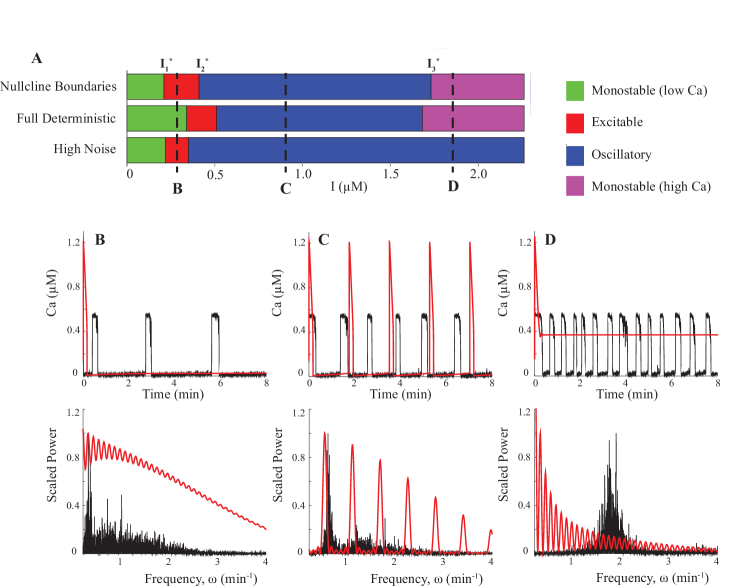
Figure 15: Noise expands the oscillatory regime. (A) Color-coded bar graph showing the dynamical regimes as a function of $I$ determined by the reduced deterministic model (Eqns. C.1-11, top), the deterministic model (Eqns. 18 and 19) for a chosen set of initial conditions (middle), and the stochastic model using the same initial conditions (bottom). (B-D) Typical dynamics (top) and scaled power spectra (bottom) for the deterministic model (red) and stochastic model (black) are shown for the $I$-values denoted by the dashed lines labeled B-D in A.

C.3 Cell-to-Cell Communication

We introduce communication into the system by allowing calcium molecules to diffuse between neighboring cells, simulating communication via gap junctions in the experiments. Doing so introduces new reactions into our model:

$$C_{i,j}\xrightleftharpoons[h]{h}C_{i+1,j},\qquad C_{i,j}\xrightleftharpoons[h]{h}C_{i,j+1},$$ (21)

where $i,j$ index cell lattice sites, and $h$ is the hopping rate of calcium ions from cell to cell. We estimate $h$ from the experimentally measured diffusion coefficient $D\sim 1$ $\mu$m²/s (see Fig. 1D of the main text). Since in our model, ions are hopping between cells on a two-dimensional lattice, $h^{-1}$ corresponds to the expected time $\ell^{2}/4D$ to diffuse a cell-to-cell distance $\ell$. Using $\ell\sim 10$$-$$20$ $\mu$m as above, we find $h\sim 0.01$$-$$0.04$ s^-1, and therefore we use $h=0.025$ s^-1.

Our calculations are done on a square lattice, where each lattice site is either empty or contains one cell, and therefore each cell can have up to four neighbors with which to communicate. Density is varied by changing the number of empty lattice sites. For each chosen density, we sample over individual realizations, in which cell locations are assigned randomly. Thus, the statistics encompass many possible spatial distributions of cells for each density.

C.4 Effects of noise and communication

Once we add noise, we can no longer distinguish the dynamic regimes (monostable, excitable, oscillatory) using the deterministic criterion, namely the number and stability of the fixed points (Fig. 14E). Instead, we define a criterion based on the trajectories themselves, similar to the procedure for the experimental trajectories. We simulate the system for a given time $T$, where $T=400$ s as in the experiments. The criterion is then:

• If the calcium level spikes zero times in $T$, the dynamics are monostable (non-oscillatory),

• If the calcium level spikes one time in $T$, the dynamics are excitable (non-oscillatory), and

• If the calcium level spikes two or more times in $T$, the dynamics are oscillatory.

When analyzing trajectories to determine ISI values, excitations separated by less than $t=5$ s are excluded, as are excitations separated by more than $t=200$ s, just as in the experimental analysis. We validate the above criterion using a complementary approach: we also compute the power spectrum of the trajectories. For periodic trajectories, the power spectrum exhibits a peak at the oscillation frequency. As shown in Fig. 15B-D, trajectories that are periodic, and thus pass the above criterion, indeed given peaked power spectra as expected.

We find that noise broadens the boundaries between dynamical regimes (Fig. 2B of the main text), and that noise shifts the boundaries between regimes (Fig. 15A, compare the bars in the middle and bottom rows). In particular, the oscillatory regime is expanded at both ends. At low values of the control parameter, noise promotes oscillations where the deterministic dynamics are excitable. At high values of the control parameter, noise promotes oscillations where the deterministic dynamics are mono-stable. Both effects have been observed in stochastic models of similar excitable systems, and are likely due to the ability of noise to cause repeated excitations and prevent damping of oscillations, respectively Mugler2016 .

C.5 Cell-to-Cell Variability

The model predicts frequency encoding, but experimental measurements show no trend in ISI values as a function of ATP concentration (Fig. 1E). We thus introduce cell-to-cell variability into the model as a possible explanation for the lack of observed frequency encoding.

Variability is introduced into our model by allowing parameters for each cell to be drawn from a distribution. All parameters $\{m_{0},n_{0},\nu,g_{0},g_{1},\pi_{1},\pi_{2},\lambda_{1},\lambda_{2},\lambda_{3},k_{-1},k_{-2},k_{-3},\alpha,\mu,h\}$ are allowed to vary from their baseline values listed in Table 1. Parameters are sampled from uniform distributions in log space such that log${}_{10}(x)\in[$log${}_{10}(\bar{x}/F)$,log${}_{10}(\bar{x}F)]$, where $\bar{x}$ is the mean value for the parameter $x$, and $F$ is a parameter that changes the strength of variability. Therefore each parameter is sampled from a distribution such that $x\in[\bar{x}/F,F\bar{x}]$.

Fig. 16 shows the ratio of the standard deviation in mean ISI values over their mean as a function of $F$. As $F$ is increased, this ratio increases until saturation occurs at $F\approx 2$. Also shown is box plot of the experimental values of this ratio, which was obtained from twelve experiments with similar density. By the saturating value $F=2$, the theoretical values lie within the experimental range; therefore we use the value $F=2$ to obtain the results that include variability in the main text.

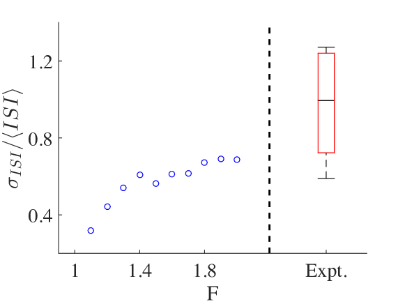
Figure 16: The effect of changing the strength of variablity parameter, $F$. The ratio of the standard deviation to the mean of the ISI, as a function of $F$. The ratio saturates above $F\approx 2$. The range of values for experiments with similar density is shown at right.

Appendix D Nearest neighbor cross-correlation analysis and computation of differential entropy

D.1 Definition

We have previously demonstrated the effectiveness of using nearest neighbor cross-correlation functions ($C_{NN}$) to characterize the calcium dynamics of collective chemosensing Sun2012 . As a result, we first study how network architecture may affect the spectrum of $C_{NN}$. For any cell $i$, we represent its calcium dynamics (fluorescent intensity profile) as $R_{i}(t)$, and define $C_{NN}$ as:

$$\dot{R}_{i}(t) =\tfrac{dR_{i}}{dt}(t)-\langle\tfrac{dR_{i}}{dt}(t)\rangle$$

$$C(\tau)_{ij} =\tfrac{1}{\sigma_{i}\sigma_{j}}\langle\dot{R}_{i}(t)\dot{R}_{j}(t+\tau)$$

$$C_{NN_{i,j}} =C(\tau=0)_{ij}\left.\right|_{D_{ij}=1}.$$ (22)

To evaluate $\frac{dR_{i}}{dt}$, we numerically differentiate the response curve $R_{i}(t)$ using the five-point stencil method; $\langle\tfrac{dR_{i}}{dt}(t)\rangle$ is the time average. Note that $\sigma^{2}_{i}$ is the variance of $R_{i}(t)$, which normalizes $C(\tau)_{ij}$ to be dimensionless. Based on Delauney triangulation of the multicellular network, topological distance $D$ can be defined for each cell pair where $D=1$ for nearest neighbors. The mean nearest neighbor cross-correlation function $\bar{C}_{NN}$ is obtained by averaging $C_{NN_{i,j}}$ over all nearest neighbor pairs $i,j$.

D.2 Statistics of nearest neighbor pairs

Table 2: Statistics of nearest neighbor pairs

[ATP]	10 $\mu$M	20 $\mu$M	50 $\mu$M	100 $\mu$M	Total
# of cells	7,055	4,245	13,078	5,062	30000
# of nearest neighbor pairs	40,596	24,462	75,092	32,222	172,372

By using Delauney triangulation coupled with the manually determined cell centers (see Fig. 7 for example), we are able to determine the connectedness of the monolayer network. In particular, we focus on the communication between nearest neighbor cells to reflect proper intercellular communication which correspond to a topological distance of $D=1$ in the triangulation. The total number of nearest neighbor pairs and cells analyzed for each ATP concentration are given in table 2.

D.3 $H_{CNN}$ of collective calcium dynamics

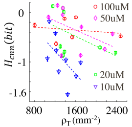
Figure 17: Differential entropy of nearest neighbor cross-correlations ($H_{cnn}$) as function of cell density at fixed fraction of cancer cells (15%$\pm$4%)

We compute the spectrum of $C_{NN_{ij}}$ using differential entropy, a scalar value that characterizes the randomness of a set of observables. The differential entropy is defined as $H=-\int\rho(x)\rho(x)dx$, where $\rho(x)$ is the probability density of a continuous variable $x$. Higher values of differential entropy are associated with broader distributions; this allows us to directly compare the spectrum of nearest neighbor cross-correlations. To avoid biasing the entropy calculation due to binning of data, the differential entropy is determined by using the $k$-nearest neighbor algorithm selim ; Loft , as described below. As shown in Fig. 17, increasing cell density decreases the differential entropy of $C_{NN}$, suggesting that higher levels of network connectivity will suppress the fluctuations in the nearest neighbor cross-correlations.

D.4 Evaluations of differential entropies

Figure 18: Evaluation of differential entropy using k-nearest neighbor method. A: Differential entropy $H_{diff}$ for normal distributions of varying standard deviations $\sigma$ and zero mean. For each $\sigma$, 1500 random variables are drawn and k-nearest neighbor method is used to calculate the corresponding differential entropy. 100 realizations (redraw the random variables) are evaluated for each $\sigma$ to calculate the mean and standard deviation of $H_{diff}$ shown as the error bars. Dashed line is the analytic result. B: Relative errors of differential entropy $H_{diff}$ calculated with varying sample sizes. For each data set of sample size $n$, n random variables are drawn from Gaussian distribution with zero mean and standard deviation equals to 1. 100 realizations are made for each sample size to calculate the relative error of $H_{diff}$. Relative error is defined as $\frac{\sqrt{<(H_{i}-H)^{2}>}}{H_{o}}$, where $H_{i}$ is the differential entropy calculated with k-nearest neighbor method at realization $i$, and $H_{o}=Ln(2\pi e)log_{2}e$. C: Histogram of $H_{CNN}$ from bootstraping a randomly selected experimental data set. $H_{CNN}$ of 1000 bootstrap realizations are calculated and the corresponding histogram is normalized to probability. Dashed line indicates the mean value.

In order to characterize the spectrum of nearest neighbor cross-correlations and inter spike intervals of the collective calcium dynamics, we have implemented a k-nearest neighbor method to calculate the differential entropy of a set of random variables. We first make benchmark tests using random variables drawn from Gaussian distributions. Since most experimental datasets contain more than 1500 elements, we compare the differential entropy calculated from 1500 Gaussian random variables with respect to the analytic results. As shown in Fig. 18A, numerical calculations agree with exact values very well. The performance of k-nearest neighbor method depends on the sample size. To evaluate the dependence, we employ k-nearest neighbor method on random variables drawn from standard normal distribution with varying sample sizes. As shown in Fig. 18B, the relative error is around 7% for sample size equals to 100, and quickly decay to less than 1% when sample size is greater than 500.

In calculating the differential entropy $H_{diff}$ using k-nearest neighbor method, every element in a dataset contribute to the final result. In order to estimate how much $H_{diff}$ fluctuates as a result of resampling, we would like to calculate $H_{diff}$ from many datasets each of which contains distinct elements drawn from the same probability distribution. However, the distribution of experiment observables are unknown. In order to perform resampling, we employ statistical bootstrap Duval1993 . As a particular example, we take a randomly selected set of nearest neighbor cross-correlations and calculated the differential entropy of 1000 bootstrap resamplings. Fig. 18C shows the probability distribution of the results. As can be seen, the fluctuation is small, and is typically less than 2%.

References

- (1) Lauffenburger, DA (2000) Cell signaling pathways as control modules: Complexity for simplicity? Proc. Natl. Acad. Sci. 97:5031–5033.
- (2) Lodish, H et al. (2000) Molecular Cell Biology, 4th edition (W. H. Freeman, New York, United States).
- (3) Barritt, G (1994) Communications Within Animal Cells (Oxford Science Publications, Oxford, UK).
- (4) Miller, MB, Bassler, BL (2001) Quorum sensing in bacteria. Annu. Rev. Microbiol. 55:165–199.
- (5) Gregor, T, Fujimoto, K, Masaki, N, Sawai, S (2010) The onset of collective behavior in social amoebae. Science 328:1021–1025.
- (6) Jones, WD, Cayirlioglu, P, Kadow, IG, Vosshall, LB (2007) Two chemosensory receptors together mediate carbon dioxide detection in drosophila. Nature 445:86–90.
- (7) Smear, M, Shusterman, R, O’Connor, R, Bozza, T, Rinberg, D (2011) Perception of sniff phase in mouse olfaction. Nature 479:397–400.
- (8) Benninger, RK, Zhang, M, Head, WS, Satin, LS, Piston, DW (2008) Gap junction coupling and calcium waves in the pancreatic islet. Biophysical journal 95:5048–5061.
- (9) Schneidman, E, II, MJB, Segev, R, Bialek, W (2006) Weak pairwise correlations imply strongly correlated network states in a neural population. Nature 440:1007–1012.
- (10) Greschner, M et al. (2011) Correlated firing among major ganglion cell types in primate retina. J. Physiol. 589:75–86.
- (11) Sun, B, Lembong, J, Normand, V, Rogers, M, Stone, HA (2012) The spatial-temporal dynamics of collective chemosensing. Proc. Nat. Aca. Sci 109:7759–7764.
- (12) Sun, B, Doclos, G, Stone, HA (2013) Network characterization of collective chemosensing. Phys. Rev. Lett. 110:158103.
- (13) Kumar, NM, Gilula, NB (1996) The gap junction communication channel. Cell 84:381–388.
- (14) Berridge, MJ, Irvine, RF (1989) Inositol phosphates and cell signalling. Nature 341:197–205.
- (15) CD, CDF, Huganir, HR, Snyderc, SH (1990) Calcium flux mediated by purified inositol 1,4,5-trisphosphate receptor in reconstituted lipid vesicles is allosterically regulated by adenine nucleotides. Proc. Natl. Acad. Sci. 87:2147–2151.
- (16) Dupont, G, Combettes, L, Bird, GS, Putney, JW (2011) Calcium oscillations. Cold Spring Harb Perspect Biol. 3:a004226.
- (17) Loewenstein, WR, Kanno, Y (1966) Intercellular communication and the control of tissue growth: lack of communication between cancer cells. Nature 209:1248–1249.
- (18) McLachlan, E, Shao, Q, Wang, HL, Langlois, S, Laird, DW (2006) Connexins act as tumor suppressors in three-dimensional mammary cell organoids by regulating differentiation and angiogenesis. Cancer Res. 66:9886–9894.
- (19) Zhou, JZ, Jiang, JX (2014) Gap junction and hemichannel-independent actions of connexins on cell and tissue functions: An update. FEBS Lett. 588:1186–1192.
- (20) Tang, Y, Othmer, HG (1995) Frequency encoding in excitable systems with applications to calcium oscillations. Proceedings of the National Academy of Sciences 92:7869–7873.
- (21) Thurley, K et al. (2014) Reliable encoding of stimulus intensities within random sequences of intracellular Ca2+ spikes. Science Signaling 7:ra59.
- (22) Woods, N, Cuthbertson, K, Cobbold, P (1985) Repetitive transient rises in cytoplasmic free calcium in hormone-stimulated hepatocytes. Nature 319:600–602.
- (23) Meyer, T, Stryer, L (1991) Calcium spiking. Annual review of biophysics and biophysical chemistry 20:153–174.
- (24) Othmer, HG, Tang, Y (1993) in Experimental and theoretical advances in biological pattern formation, eds Othmer, HG, Maini, PK, Murray, JD (Springer US).
- (25) Meyer, T, Stryer, L (1988) Molecular model for receptor-stimulated calcium spiking. Proc. Natl. Acad. Sci. 85:5051–5055.
- (26) Politi, A, Gaspers, LD, Thomas, AP, Höfer, T (2006) Models of ip3 and ca2+ oscillations: Frequency encoding and identification of underlying feedbacks. Biophys. J. 90:3120–3133.
- (27) Swillens, S, Dupont, G, Combettes, L, Champeil, P (1999) From calcium blips to calcium puffs: Theoretical analysis of the requirements for interchannel communication. Proc. Natl. Acad. Sci. 96:13750–13755.
- (28) Falcke, M (2004) Reading the patterns in living cells the physics of ca2 signaling. Adv. Physics 53:255–440.
- (29) Gillespie, DT (1977) Exact stochastic simulation of coupled chemical reactions. The journal of physical chemistry 81:2340–2361.
- (30) Meister, M (1996) Multineuronal codes in retinal signaling. Proc. Natl. Acad. Sci. 93:609–614.
- (31) Schnizer, MJ, Meister, M (2003) Multineuronal firing patterns in the signal from eye to brain. Neuron 37:499–511.
- (32) Janmey, PA, Miller, RT (2011) Mechanisms of mechanical signaling in development and disease. Journal of cell science 124:9–18.
- (33) Abbaci, M, Barberi-Heyob, M, Blondel, W, Guillemin, F, Didelon, J (2008) Advantages and limitations of commonly used methods to assay the molecular permeability of gap junctional intercellular communication. BioTechniques 45:33–62.
- (34) Schwiebert, EM, Zsembery, A (2003) Extracellular atp as a signaling molecule for epithelial cells. Biochimica et Biophysica Acta (BBA)-Biomembranes 1615:7–32.
- (35) Falzoni, S, Donvito, G, Di Virgilio, F (2013) Detecting adenosine triphosphate in the pericellular space. Interface Focus 3:20120101.
- (36) Trabanelli, S et al. (2012) Extracellular atp exerts opposite effects on activated and regulatory cd4+ t cells via purinergic p2 receptor activation. The Journal of Immunology 189:1303–1310.
- (37) Pellegatti, P et al. (2008) Increased level of extracellular atp at tumor sites: in vivo imaging with plasma membrane luciferase. PloS one 3:e2599.
- (38) Mehta, P, Gregor, T (2010) Approaching the molecular origins of collective dynamics in oscillating cell populations. Current opinion in genetics & development 20:574–580.
- (39) De Monte, S, d’Ovidio, F, Dano, S, Sorensen, PG (2007) Dynamical quorum sensing: Population density encoded in cellular dynamics. Proceedings of the National Academy of Sciences 104:18377–18381.
- (40) Taylor, AF, Tinsley, MR, Wang, F, Huang, Z, Showalter, K (2009) Dynamical quorum sensing and synchronization in large populations of chemical oscillators. Science 323:614–617.
- (41) de Ronde, W, Tostevin, F, Ten Wolde, PR (2011) Multiplexing biochemical signals. Physical review letters 107:048101.
- (42) Cheong, R, Rhee, A, Wang, CJ, Nemenman, I, Levchenko, A (2011) Information transduction capacity of noisy biochemical signaling networks. science 334:354–358.
- (43) Selimkhanov, J et al. (19652014) Accurate information transmission through dynamic biochemical signaling networks. Science 346:1370–1373.
- (44) Tay, S et al. (2010) Single-cell nf-[kgr] b dynamics reveal digital activation and analogue information processing. Nature 466:267–271.
- (45) Kellogg, RA, Tay, S (2015) Noise facilitates transcriptional control under dynamic inputs. Cell 160:381–392.
- (46) Mora, T, Bialek, W (2011) Are biological systems poised at criticality? Journal of Statistical Physics 144:268–302.
- (47) Krotov, D, Dubuis, JO, Gregor, T, Bialek, W (2014) Morphogenesis at criticality. Proceedings of the National Academy of Sciences 111:3683–3688.
- (48) Hidalgo, J et al. (2014) Information-based fitness and the emergence of criticality in living systems. Proceedings of the National Academy of Sciences 111:10095–10100.
- (49) Gillespie, DT (2001) Approximate accelerated stochastic simulation of chemically reacting systems. The Journal of Chemical Physics 115:1716–1733.
- (50) Rathinam, M, Petzold, LR, Cao, Y, Gillespie, DT (2003) Stiffness in stochastic chemically reacting systems: The implicit tau-leaping method. The Journal of Chemical Physics 119:12784–12794.
- (51) Cao, Y, Gillespie, DT, Petzold, LR (2006) Efficient step size selection for the tau-leaping simulation method. The Journal of chemical physics 124:044109.
- (52) Cao, Y, Gillespie, DT, Petzold, LR (2007) Adaptive explicit-implicit tau-leaping method with automatic tau selection. The Journal of chemical physics 126:224101.
- (53) Garcia, D (2010) Robust smoothing of gridded data in one and higher dimensions with missing values. Computational statistics & data analysis 54:1167–1178.
- (54) Wang, S, Alousi, AA, Thompson, SH (1995) The lifetime of inositol 1, 4, 5-trisphosphate in single cells. The Journal of general physiology 105:149–171.
- (55) Mugler, A et al. (2016) Noise expands the response range of the bacillus subtilis competence circuit. PLoS Computational Biology Accepted.
- (56) Selimkhanov, J et al. (2014) Accurate information transmission through dynamic biochemical signaling networks. Science 346:1370–1373.
- (57) Loftsgaarden, DO, Quesenberry, CP et al. (1965) A nonparametric estimate of a multivariate density function. The Annals of Mathematical Statistics 36:1049–1051.
- (58) Mooney, CZ, Duval, RD, Duval, R (1993) Bootstrapping: A nonparametric approach to statistical inference (Sage) No. 94-95.