Maximum Likelihood Estimates for
Gaussian Mixtures Are Transcendental

Abstract

Gaussian mixture models are central to classical statistics, widely used in the information sciences, and have a rich mathematical structure. We examine their maximum likelihood estimates through the lens of algebraic statistics. The MLE is not an algebraic function of the data, so there is no notion of ML degree for these models. The critical points of the likelihood function are transcendental, and there is no bound on their number, even for mixtures of two univariate Gaussians.

1 Introduction

The primary purpose of this paper is to demonstrate the result stated in the title:

Theorem 1.1

The maximum likelihood estimators of Gaussian mixture models are transcendental functions. More precisely, there exist rational samples $x_{1},x_{2},\ldots,x_{N}$ in $\mathbb{Q}^{n}$ whose maximum likelihood parameters for the mixture of two $n$-dimensional Gaussians are not algebraic numbers over $\mathbb{Q}$.

The principle of maximum likelihood (ML) is central to statistical inference. Most implementations of ML estimation employ iterative hill-climbing methods, such as expectation maximization (EM). These can rarely certify that a globally optimal solution has been reached. An alternative paradigm, advanced by algebraic statistics [8], is to find the ML estimator (MLE) by solving the likelihood equations. This is only feasible for small models, but it has the benefit of being exact and certifiable. An important notion in this approach is the ML degree, which is defined as the algebraic degree of the MLE as a function of the data. This rests on the premise that the likelihood equations are given by polynomials.

Many models used in practice, such as exponential families for discrete or Gaussian observations, can be represented by polynomials. Hence, they have an ML degree that serves as an upper bound for the number of isolated local maxima of the likelihood function, independently of the sample size and the data. The ML degree is an intrinsic invariant of a statistical model, with interesting geometric and topological properties [13]. The notion has proven useful for characterization of when MLEs admit a ‘closed form’ [19]. When the ML degree is moderate, these exact tools are guaranteed to find the optimal solution to the ML problem [5, 12].

However, the ML degree of a statistical model is only defined when the MLE is an algebraic function of the data. Theorem 1.1 means that there is no ML degree for Gaussian mixtures. It also highlights a fundamental difference between likelihood inference and the method of moments [3, 10, 15]. The latter is a computational paradigm within algebraic geometry, that is, it is based on solving polynomial equations. ML estimation being transcendental means that likelihood inference in Gaussian mixtures is outside the scope of algebraic geometry.

The proof of Theorem 1.1 will appear in Section 2. In Section 3 we shed further light on the transcendental nature of Gaussian mixture models. We focus on mixtures of two univariate Gaussians, the model given in (1) below, and we present a family of data points on the real line such that the number of critical points of the corresponding log-likelihood function (2) exceeds any bound.

While the MLE for Gaussian mixtures is transcendental, this does not mean that exact methods are not available. Quite to the contrary. Work of Yap and his collaborators in computational geometry [6, 7] convincingly demonstrates this. Using root bounds from transcendental number theory, they provide certified answers to geometric optimization problems whose solutions are known to be transcendental. Theorem 1.1 opens up the possibility of transferring these techniques to statistical inference. In our view, Gaussian mixtures are an excellent domain of application for certified computation in numerical analytic geometry.

2 Reaching Transcendence

Transcendental number theory [2, 11] is a field that furnishes tools for deciding whether a given real number $\tau$ is a root of a nonzero polynomial in $\mathbb{Q}[t]$. If this holds then $\tau$ is algebraic; otherwise $\tau$ is transcendental. For instance, $\sqrt{2}+\sqrt{7}=4.059964873...$ is algebraic, and so are the parameter estimates computed by Pearson in his 1894 study of crab data [15]. By contrast, the famous constants $\pi=3.141592653...$ and $e=2.718281828...$ are transcendental. Our proof will be based on the following classical result. A textbook reference is [2, Theorem 1.4]:

Theorem 2.1 (Lindemann-Weierstrass)

If $u_{1},\ldots,u_{r}$ are distinct algebraic numbers then $e^{u_{1}},\ldots,e^{u_{r}}$ are linearly independent over the algebraic numbers.

For now, consider the case of $n=1$, that is, mixtures of two univariate Gaussians. We allow mixtures with arbitrary means and variances. Our model then consists of all probability distributions on the real line $\mathbb{R}$ with density

$$f_{\alpha,\mu,\sigma}(x)=\frac{1}{\sqrt{2\pi}}\cdot\biggl{[}\frac{\alpha}{\sigma_{1}}\,\exp\Bigl{(}-\frac{(x-\mu_{1})^{2}}{2\sigma_{1}^{2}}\Bigr{)}\,+\,\frac{1-\alpha}{\sigma_{2}}\,\exp\Bigl{(}-\frac{(x-\mu_{2})^{2}}{2\sigma_{2}^{2}}\Bigr{)}\biggr{]}\enspace.$$ (1)

It has five unknown parameters, namely, the means $\mu_{1},\mu_{2}\in\mathbb{R}$, the standard deviations $\sigma_{1},\sigma_{2}>0$, and the mixture weight $\alpha\in[0,1]$. The aim is to estimate the five model parameters from a collection of data points $x_{1},x_{2},\ldots,x_{N}\in\mathbb{R}$.

The log-likelihood function of the model (1) is

$$\ell(\alpha,\mu_{1},\mu_{2},\sigma_{1},\sigma_{2})\,\,=\,\,\sum_{i=1}^{N}\log f_{\alpha,\mu,\sigma}(x_{i})\enspace.$$ (2)

This is a function of the five parameters, while $x_{1},\ldots,x_{N}$ are fixed constants.

The principle of maximum likelihood suggests to find estimates by maximizing the function $\ell$ over the five-dimensional parameter space $\Theta=[0,1]\times\mathbb{R}^{2}\times\mathbb{R}^{2}_{>0}$.

Remark 1

The log-likelihood function $\ell$ in (2) is never bounded above. To see this, we argue as in [4, Section 9.2.1]. Set $N=2$, fix arbitrary values $\alpha_{0}\in[0,1]$, $\mu_{20}\in\mathbb{R}$ and $\sigma_{20}>0$, and match the first mean to the first data point $\mu_{1}=x_{1}$. The remaining function of one unknown $\sigma_{1}$ equals

$$\ell(\alpha_{0},x_{1},\mu_{20},\sigma_{1},\sigma_{20})\,\geq\,\log\biggl{[}\frac{\alpha_{0}}{\sigma_{1}}\,+\,\frac{1-\alpha_{0}}{\sigma_{20}}\,\exp\Bigl{(}-\frac{(x_{1}-\mu_{20})^{2}}{2\sigma_{20}^{2}}\Bigr{)}\biggr{]}\,+\,\text{const}\enspace.$$

The lower bound tends to $\infty$ as $\sigma_{1}\to 0$.

Remark 1 means that there is no global solution to the MLE problem. This is remedied by restricting to a subset of the parameter space $\Theta$. In practice, maximum likelihood for Gaussian mixtures means computing local maxima of the function $\ell$. These are found numerically by a hill climbing method, such as the EM algorithm, with particular choices of starting values. See Section 3. This method is implemented, for instance, in the R package MCLUST [9]. In order for Theorem 1.1 to cover such local maxima, we prove the following statement:

There exist samples $x_{1},\ldots,x_{N}\in\mathbb{Q}$ such that every non-trivial critical point $(\hat{\alpha},\hat{\mu}_{1},\hat{\mu}_{2},\hat{\sigma}_{1},\hat{\sigma}_{2})$ of the log-likelihood function $\ell$ in the domain $\Theta$ has at least one transcendental coordinate.

Here, a critical point is non-trivial if it yields an honest mixture, i.e. a distribution that is not Gaussian. By the identifiability results of [20], this happens if and only if the estimate $(\hat{\alpha},\hat{\mu}_{1},\hat{\mu}_{2},\hat{\sigma}_{1},\hat{\sigma}_{2})$ satisfies $0<\hat{\alpha}<1$ and $(\hat{\mu}_{1},\hat{\sigma}_{1})\not=(\hat{\mu}_{2},\hat{\sigma}_{2})$.

Remark 2

The log-likelihood function always has some algebraic critical points, for any $x_{1},\dots,x_{N}\in\mathbb{Q}$. Indeed, if we define the empirical mean and variance as

$$\bar{x} =\frac{1}{N}\sum_{i=1}^{N}x_{i}\,, s^{2} =\frac{1}{N}\sum_{i=1}^{N}(x_{i}-\bar{x})^{2}\enspace,$$

then any point $(\hat{\alpha},\hat{\mu}_{1},\hat{\mu}_{2},\hat{\sigma}_{1},\hat{\sigma}_{2})$ with $\hat{\mu}_{1}=\hat{\mu}_{2}=\bar{x}$ and $\hat{\sigma}_{1}=\hat{\sigma}_{2}=s$ is critical. This gives a Gaussian distribution with mean $\bar{x}$ and variance $s^{2}$, so it is trivial.

Proof (of Theorem 1.1)

First, we treat the univariate case. Consider the partial derivative of (2) with respect to the mixture weight $\alpha$:

$$\frac{\partial\ell}{\partial\alpha} \;=\;\sum_{i=1}^{N}\frac{1}{f_{\alpha,\mu,\sigma}(x_{i})}\cdot\frac{1}{\sqrt{2\pi}}\left[\frac{1}{\sigma_{1}}\exp\Bigl{(}-\frac{(x_{i}-\mu_{1})^{2}}{2\sigma_{1}^{2}}\Bigr{)}\;-\;\frac{1}{\sigma_{2}}\exp\Bigl{(}-\frac{(x_{i}-\mu_{2})^{2}}{2\sigma_{2}^{2}}\Bigr{)}\right].$$ (3)

Clearing the common denominator

$$\sqrt{2\pi}\cdot\prod_{i=1}^{N}f_{\alpha,\mu,\sigma}(x_{i})\enspace,$$

we see that $\partial\ell/\partial\alpha=0$ if and only if

$$\sum_{i=1}^{N} \left[\frac{1}{\sigma_{1}}\,\exp\Bigl{(}-\frac{(x_{i}-\mu_{1})^{2}}{2\sigma_{1}^{2}}\Bigr{)}\;-\;\frac{1}{\sigma_{2}}\,\exp\Bigl{(}-\frac{(x_{i}-\mu_{2})^{2}}{2\sigma_{2}^{2}}\Bigr{)}\right]$$

$$\times\prod_{j\not=i}\biggl{[}\frac{\alpha}{\sigma_{1}}\,\exp\Bigl{(}-\frac{(x_{j}-\mu_{1})^{2}}{2\sigma_{1}^{2}}\Bigr{)}\,+\,\frac{1-\alpha}{\sigma_{2}}\,\exp\Bigl{(}-\frac{(x_{j}-\mu_{2})^{2}}{2\sigma_{2}^{2}}\Bigr{)}\biggr{]}\;=\;0\enspace.$$ (4)

Letting $\alpha_{1}=\alpha$ and $\alpha_{2}=1-\alpha$, we may rewrite the left-hand side of (4) as

$$\sum_{i=1}^{N} \left[\sum_{k_{i}=1}^{2}\frac{(-1)^{k_{i}-1}}{\sigma_{k_{i}}}\,\exp\Bigl{(}-\frac{(x_{i}-\mu_{k_{i}})^{2}}{2\sigma_{k_{i}}^{2}}\Bigr{)}\right]\prod_{j\not=i}\left[\sum_{k_{j}=1}^{2}\frac{\alpha_{k_{j}}}{\sigma_{k_{j}}}\,\exp\Bigl{(}-\frac{(x_{j}-\mu_{k_{j}})^{2}}{2\sigma_{k_{j}}^{2}}\Bigr{)}\right].$$ (5)

We expand the products, collect terms, and set $N_{i}(k)=|\{j:k_{j}=i\}|$. With this, the partial derivative $\partial\ell/\partial\alpha$ is zero if and only if the following vanishes:

$$\sum_{i=1}^{N}\sum_{k\in\{1,2\}^{N}}\!\!\!\exp\!\left(\!-\sum_{j=1}^{N}\frac{(x_{j}-\mu_{k_{j}})^{2}}{2\sigma_{k_{j}}^{2}}\right)\!(-1)^{k_{i}-1}\alpha^{|\{j\not=i:k_{j}=1\}|}(1{-}\alpha)^{|\{j\not=i:k_{j}=2\}|}\left(\prod_{j=1}^{N}\frac{1}{\sigma_{k_{j}}}\right)$$

$$\!=\!\!\!\sum_{k\in\{1,2\}^{N}}\!\!\!\!\exp\!\left(\!-\sum_{j=1}^{N}\!\frac{(x_{j}-\mu_{k_{j}})^{2}}{2\sigma_{k_{j}}^{2}}\right)\!\!\left(\prod_{j=1}^{N}\frac{1}{\sigma_{k_{j}}}\right)\!\sum_{i=1}^{N}(-1)^{k_{i}-1}\alpha^{|\{j\not=i:k_{j}=1\}|}(1-\alpha)^{|\{j\not=i:k_{j}=2\}|}$$

$$\!\!=\!\!\sum_{k\in\{1,2\}^{N}}\!\!\!\!\exp\!\left(-\sum_{j=1}^{N}\frac{(x_{j}-\mu_{k_{j}})^{2}}{2\sigma_{k_{j}}^{2}}\right)\!\!\left(\prod_{j=1}^{N}\frac{1}{\sigma_{k_{j}}}\right)\!\alpha^{N_{1}(k)-1}(1{-}\alpha)^{N_{2}(k)-1}\left[{N_{1}(k)(1{-}\alpha)\atop+N_{2}(k)(-\alpha)}\right]$$

$$\!\!=\!\!\sum_{k\in\{1,2\}^{N}}\!\!\!\!\exp\!\left(\!-\sum_{j=1}^{N}\frac{(x_{j}-\mu_{k_{j}})^{2}}{2\sigma_{k_{j}}^{2}}\right)\!\!\left(\prod_{j=1}^{N}\frac{1}{\sigma_{k_{j}}}\right)\alpha^{N_{1}(k)-1}(1-\alpha)^{N-N_{1}(k)-1}(N_{1}(k)-N\alpha)\enspace.\,\,\,$$

Let $(\hat{\alpha},\hat{\mu}_{1},\hat{\mu}_{2},\hat{\sigma}_{1},\hat{\sigma}_{2})$ be a non-trivial isolated critical point of the likelihood function. This means that $0<\hat{\alpha}<1$ and $(\hat{\mu}_{1},\hat{\sigma}_{1})\not=(\hat{\mu}_{2},\hat{\sigma}_{2})$. This point depends continuously on the choice of the data $x_{1},x_{2},\ldots,x_{N}$. By moving the vector with these coordinates along a general line in $\mathbb{R}^{N}$, the mixture parameter $\hat{\alpha}$ moves continuously in the critical equation $\partial\ell/\partial\alpha=0$ above. By the Implicit Function Theorem, it takes on all values in some open interval of $\mathbb{R}$, and we can thus choose our data points $x_{i}$ general enough so that $\hat{\alpha}$ is not an integer multiple of $1/N$. We can further ensure that the last sum above is a $\mathbb{Q}(\alpha)$-linear combination of exponentials with nonzero coefficients.

Suppose that $(\hat{\alpha},\hat{\mu}_{1},\hat{\mu}_{2},\hat{\sigma}_{1},\hat{\sigma}_{2})$ is algebraic. The Lindemann-Weierstrass Theorem implies that the arguments of ${\rm exp}$ are all the same. Then the $2^{N}$ numbers

$$\sum_{j=1}^{N}\frac{(x_{j}-\hat{\mu}_{k_{j}})^{2}}{2{\hat{\sigma}_{k_{j}}}^{2}}\,,\qquad k\in\{1,2\}^{N},$$

are all identical. However, for $N\geq 3$, and for general choice of data $x_{1},\dots,x_{N}$ as above, this can only happen if $(\hat{\mu}_{1},\hat{\sigma}_{1})=(\hat{\mu}_{2},\hat{\sigma}_{2})$. This contradicts our hypothesis that the critical point is non-trivial. We conclude that all non-trivial critical points of the log-likelihood function (2) are transcendental.

In the multivariate case, the model parameters comprise the mixture weight $\alpha\in[0,1]$, mean vectors $\mu_{1},\mu_{2}\in\mathbb{R}^{n}$ and positive definite covariance matrices $\Sigma_{1},\Sigma_{2}\in\mathbb{R}^{n}$. Arguing as above, if a non-trivial critical $(\hat{\alpha},\hat{\mu}_{1},\hat{\mu}_{2},\hat{\Sigma}_{1},\hat{\Sigma}_{2})$ is algebraic, then the Lindemann-Weierstrass Theorem implies that the numbers

$$\sum_{j=1}^{N}(x_{j}-\hat{\mu}_{k_{j}})^{T}\hat{\Sigma}_{k_{j}}^{-1}(x_{j}-\hat{\mu}_{k_{j}})\,,\qquad k\in\{1,2\}^{N}\,,$$

are all identical. For $N$ sufficiently large and a general choice of $x_{1},\dots,x_{N}$ in $\mathbb{R}^{n}$, the $2^{N}$ numbers are identical only if $(\hat{\mu}_{1},\hat{\Sigma}_{1})=(\hat{\mu}_{2},\hat{\Sigma}_{2})$. Again, this constitutes a contradiction to the hypothesis that $(\hat{\alpha},\hat{\mu}_{1},\hat{\mu}_{2},\hat{\Sigma}_{1},\hat{\Sigma}_{2})$ is non-trivial. ∎

Many variations and specializations of the Gaussian mixture model are used in applications. In the case $n=1$, the variances are sometimes assumed equal, so $\sigma_{1}=\sigma_{2}$ for the above two-mixture. This avoids the issue of an unbounded likelihood function (as long as $N\geq 3$). Our proof of Theorem 1.1 applies to this setting. In higher dimensions $(n\geq 2$), the covariance matrices are sometimes assumed arbitrary and distinct, sometimes arbitrary and equal, but often also have special structure such as being diagonal. Various default choices are discussed in the paper [9] that introduces the R package MCLUST. Our results imply that maximum likelihood estimation is transcendental for all these MCLUST models.

Example 1

We illustrate Theorem 1.1 for a specialization of (1) obtained by fixing three parameters: $\mu_{2}=0$ and $\sigma_{1}=\sigma_{2}=1/\sqrt{2}$. The remaining two free parameters are $\alpha$ and $\mu=\mu_{1}$. We take only $N=2$ data points, namely $x_{1}=0$ and $x_{2}=x>0$. Omitting an additive constant, our log-likelihood function equals

$$\ell(\alpha,\mu)\,\,\,=\,\,\,{\rm log}\bigl{(}\alpha\cdot e^{-\mu^{2}}+(1-\alpha)\bigr{)}\,\,+\,\,{\rm log}\bigl{(}\alpha\cdot e^{-(\mu-x)^{2}}+(1-\alpha)\cdot e^{-x^{2}}\bigr{)}\enspace.$$ (6)

For a concrete example take $x=2$. The graph of (6) for this choice is shown in Figure 1. By maximizing $\ell(\alpha,\mu)$ numerically, we find the parameter estimates

$$\hat{\alpha}=0.50173262959803874...\quad\hbox{and}\quad\hat{\mu}\,=\,1.95742494230308167...$$ (7)

Our technique can be applied to prove that $\hat{\alpha}$ and $\hat{\mu}$ are transcendental over $\mathbb{Q}$. We illustrate it for $\hat{\mu}$.

For any $x\in\mathbb{R}$, the function $\ell(\alpha,\mu)$ is bounded from above and achieves its maximum on $[0,1]\times\mathbb{R}$. If $x>0$ is large, then any global maximum $(\hat{\alpha},\hat{\mu})$ of $\ell$ is in the interior of $[0,1]\times\mathbb{R}$ and satisfies $0<\hat{\mu}\leq x$. According to a Mathematica computation, the choice $x\geq 1.56125...$ suffices for this. Assume that this holds. Setting the two partial derivatives equal to zero and eliminating the unknown $\alpha$ in a further Mathematica computation, the critical equation for $\mu$ is found to be

$$(x-\mu)e^{\mu^{2}}\,-\,x\,+\,\mu e^{-\mu(2x-\mu)}\,\;=\,\;0\enspace.$$ (8)

Suppose for contradiction that both $x$ and $\hat{\mu}$ are algebraic numbers over $\mathbb{Q}$. Since $0<\hat{\mu}\leq x$, we have $-\hat{\mu}(2x-\hat{\mu})<0<\hat{\mu}^{2}$. Hence $\,u_{1}=\hat{\mu}^{2}$, $\,u_{2}=0\,$ and $\,u_{3}=-\hat{\mu}(2x-\hat{\mu})\,$ are distinct algebraic numbers. The Lindemann-Weierstrass Theorem implies that $e^{u_{1}},e^{u_{2}}$ and $e^{u_{3}}$ are linearly independent over the field of algebraic numbers. However, from (8) we know that

$$(x-\hat{\mu})\cdot e^{u_{1}}\,-\,x\cdot e^{u_{2}}\,+\,\hat{\mu}\cdot e^{u_{3}}\,\,\;=\,\,\;0\enspace.$$

This is a contradiction. We conclude that the number $\hat{\mu}$ is transcendental over $\mathbb{Q}$.

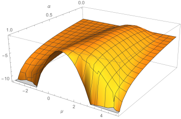
Figure 1: Graph of the log-likelihood function for two data points $x_{1}=0$ and $x_{2}=2$.

3 Many Critical Points

Theorem 1.1 shows that Gaussian mixtures do not admit an ML degree. This raises the question of how to find any bound for the number of critical points.

Problem 1

Does there exist a universal bound on the number of non-trivial critical points for the log-likelihood function of the mixture of two univariate Gaussians? Or, can we find a sequence of samples on the real line such that the number of non-trivial critical points increases beyond any bound?

We shall resolve this problem by answering the second question affirmatively. The idea behind our solution is to choose a sample consisting of many well-separated clusters of size $2$. Then each cluster gives rise to a distinct non-trivial critical point $(\hat{\alpha},\hat{\mu}_{1},\hat{\mu}_{2},\hat{\sigma}_{1},\hat{\sigma}_{2})$ of the log-likelihood function $\ell$ from (2). We propose one particular choice of data, but many others would work too.

Theorem 3.1

Fix sample size $N=2K$ for $K\geq 2$, and take the ordered sample $(x_{1},\ldots,x_{2K})=(1,1.2,\,2,2.2,\,\ldots,K,K{+}0.2)$. Then, for each $k\in\{1,\ldots,K\}$, the log-likelihood function $\ell$ from (2) has a non-trivial critical point with $k<\hat{\mu}_{1}<k+0.2$. Hence, there are at least $K$ non-trivial critical points.

Before turning to the proof, we offer a numerical illustration.

Table 1: Seven critical points of the log-likelihood function in Theorem 3.1 with $K=7$.

$k$	$\alpha$	$\mu_{1}$	$\mu_{2}$	$\sigma_{1}$	$\sigma_{2}$	log-likelihood
1	0.1311958	1.098998	4.553174	0.09999497	1.746049	-27.2918782147578
2	0.1032031	2.097836	4.330408	0.09997658	1.988948	-28.6397463805501
3	0.07883084	3.097929	4.185754	0.09997856	2.06374	-29.1550277534757
4	0.06897294	4.1	4.1	0.1	2.07517	-29.2858981551065
5	0.07883084	5.102071	4.014246	0.09997856	2.06374	-29.1550277534757
6	0.1032031	6.102164	3.869592	0.09997658	1.988948	-28.6397463805501
7	0.1311958	7.101002	3.646826	0.09999497	1.746049	-27.2918782147578

Example 2

For $K=7$, we have $N=14$ data points in the interval $[1,7.2]$. Running the EM algorithm (as explained in the proof of Theorem 3.1 below) yields the non-trivial critical points reported in Table 1. Their $\mu_{1}$ coordinates are seen to be close to the cluster midpoints $k+0.1$ for all $k$. The observed symmetry under reversing the order of the rows also holds for all larger $K$.

Our proof of Theorem 3.1 will be based on the EM algorithm. We first recall this algorithm. Let $f_{\alpha,\mu,\sigma}$ be the mixture density from (1), and let

$$f_{j}(x)\,\,=\,\,\frac{1}{\sqrt{2\pi}\,\sigma_{j}}\,\exp\Bigl{(}-\frac{(x-\mu_{j})^{2}}{2\sigma_{j}^{2}}\Bigr{)},\quad j=1,2\enspace,$$

be the two Gaussian component densities. Define

$$\gamma_{i}=\frac{\alpha\cdot f_{1}(x_{i})}{f_{\alpha,\mu,\sigma}(x_{i})}\enspace,$$ (9)

which can be interpreted as the conditional probability that data point $x_{i}$ belongs to the first mixture component. Further, define $N_{1}=\sum_{i=1}^{N}\gamma_{i}$ and $N_{2}=N-N_{1}$, which are expected cluster sizes. Following [4, Section 9.2.2], the likelihood equations for our model can be written in the following fixed-point form:

$$\alpha =\frac{N_{1}}{N}\,,$$ (10)

$$\mu_{1} =\frac{1}{N_{1}}\sum_{i=1}^{N}\gamma_{i}x_{i}\,, \mu_{2} =\frac{1}{N_{2}}\sum_{i=1}^{N}(1-\gamma_{i})x_{i}\,,$$ (11)

$$\sigma_{1} =\frac{1}{N_{1}}\sum_{i=1}^{N}\gamma_{i}(x_{i}-\mu_{1})^{2}\,, \sigma_{2} =\frac{1}{N_{2}}\sum_{i=1}^{N}(1-\gamma_{i})(x_{i}-\mu_{2})^{2}\enspace.$$ (12)

In the present context, the EM algorithm amounts to solving these equations iteratively. More precisely, consider any starting point $(\alpha,\mu_{1},\mu_{2},\sigma_{1},\sigma_{2})$. Then the E-step (“expectation”) computes the estimated frequencies $\gamma_{i}$ via (9). In the subsequent M-step (“maximization”), one obtains a new parameter vector $(\alpha,\mu_{1},\mu_{2},\sigma_{1},\sigma_{2})$ by evaluating the right-hand sides of the equations (10)-(12). The two steps are repeated until a fixed point is reached, up to the desired numerical accuracy. The updates never decrease the log-likelihood. For our problem it can be shown that the algorithm will converge to a critical point; see e.g. [16].

Proof (of Theorem 3.1)

Fix $k\in\{1,\dots,K\}$. We choose starting parameter values to suggest that the pair $(x_{2k-1},x_{2k})=(k,k+0.2)$ belongs to the first mixture component, while the rest of the sample belongs to the second. Explicitly, we set

$$\alpha =\frac{2}{N}=\frac{1}{K}\,,$$

$$\mu_{1} =k+0.1\,, \mu_{2} =\frac{K^{2}+1.2K-2k-0.2}{2(K-1)}\,,$$

$$\sigma_{1} =0.1\,, \sigma_{2} =\frac{\sqrt{\frac{1}{12}K^{4}-\frac{1}{3}K^{3}+(k-\frac{43}{75})K^{2}-(k^{2}-k+\frac{14}{75})K+0.01}}{K-1}\enspace.$$

We shall argue that, when running the EM algorithm, the parameters will always stay close to these starting values. Specifically, we claim that throughout all EM iterations, the parameter values satisfy the inequalities

$$\frac{1}{4K}\leq\alpha\leq\frac{1}{K}\,, 0.09\leq\mu_{1}-k\leq 0.11\,, 0.099\leq\sigma_{1}\leq 0.105\,,$$ (13)

$$\frac{K}{2}+0.1\,\,\leq\,\, \mu_{2}\leq\frac{K}{2}+1.1\,,$$ (14)

$$\sqrt{\frac{K^{2}}{12}-\frac{K}{6}+0.01}\,\,\leq\,\, \sigma_{2}\leq\sqrt{\frac{K^{2}}{12}+\frac{K}{12}+0.01}\enspace.$$ (15)

The starting values proposed above obviously satisfy the inequalities in (13), and it is not difficult to check that (14) and (15) are satisfied as well. To prove the theorem, it remains to show that (13)-(15) continue to hold after an EM update.

In the remainder, we assume that $K>22$. For smaller values of $K$ the claim of the theorem can be checked by running the EM algorithm. In particular, for $K>3$, the second standard deviation satisfies the simpler bounds

$$\frac{K}{\sqrt{12}}-\frac{\sqrt{3}}{5}\leq\sigma_{2}\leq\frac{K}{\sqrt{12}}+\frac{\sqrt{3}}{12}\enspace.$$ (16)

A key property is that the quantity $\gamma_{i}$, computed in the E-step, is always very close to zero for $i\neq 2k-1,2k$. To see why, rewrite (9) as

$$\gamma_{i}=\frac{1}{1+\frac{1-\alpha}{\alpha}\frac{f_{2}(x_{i})}{f_{1}(x_{i})}}=\frac{1}{1+\frac{1-\alpha}{\alpha}\frac{\sigma_{1}}{\sigma_{2}}\exp\left\{\frac{1}{2}\left((\frac{x_{i}-\mu_{1}}{\sigma_{1}})^{2}-(\frac{x_{i}-\mu_{2}}{\sigma_{2}})^{2}\right)\right\}}\enspace.$$

Since $\alpha\leq 1/K$, we have $\frac{1-\alpha}{\alpha}\geq K-1$. On the other hand, $\frac{\sigma_{1}}{\sigma_{2}}\geq\frac{0.099}{K/\sqrt{12}+\sqrt{3}/12}$. Using that $K>22$, their product is thus bounded below by 0.3209. Turning to the exponential term, the second inequality in (13) implies that $|x_{i}-\mu_{1}|\geq 0.89$ for $i=2k-2$ or $i=2k+1$, which index the data points closest to the $k$th pair.

Using (16), we obtain

$$\left(\frac{x_{i}-\mu_{1}}{\sigma_{1}}\right)^{2}-\left(\frac{x_{i}-\mu_{2}}{\sigma_{2}}\right)^{2}\,\,\geq\,\,\left(\frac{0.89}{0.105}\right)^{2}-\left(\frac{K/2+0.1}{K/\sqrt{12}-\sqrt{3}/5}\right)^{2}\,\,\geq\,\,67.86\enspace.$$

From $e^{33.93}>5.4\cdot 10^{14}$, we deduce that $\gamma_{i}<10^{-14}$. The exponential term becomes only smaller as the considered data point $x_{i}$ move away from the $k$th pair. As $|i-(2k-1/2)|$ increases, $\gamma_{i}$ decreases and can be bounded above by a geometric progression starting at $10^{-14}$ and with ratio $10^{-54}$. This makes $\gamma_{i}$ with $i\neq 2k,2k-1$ negligible. Indeed, from the limit of geometric series, we have

$$s_{1} =\sum_{i\not=2k-1,2k}\gamma_{i}\,\,<\,\,10^{-13}\enspace,$$ (17)

and similarly, $s_{2}=\sum_{i\not=2k-1,2k}\gamma_{i}(x_{i}-k)$ satisfies

$$\!\!|s_{2}|\,=\,\left|\gamma_{2k-2}(-0.8)+\gamma_{2k+1}(1)+\gamma_{2k-3}(-1)+\gamma_{2k+2}(1.2)+\ldots\right|\,<\,10^{-13}\enspace.$$ (18)

The two sums $s_{1}$ and $s_{2}$ are relevant for the M-step.

The probabilities $\gamma_{2k-1}$ and $\gamma_{2k}$ give the main contribution to the averages that are evaluated in the M-step. They satisfy $\,0.2621\leq\gamma_{2k-1},\gamma_{2k}\leq 0.9219$. Moreover, we may show that the values of $\gamma_{2k-1}$ and $\gamma_{2k}$ are similar, namely:

$$0.8298\leq\frac{\gamma_{2k-1}}{\gamma_{2k}}\leq 1.2213\enspace,$$ (19)

which we prove by writing

$$\frac{\gamma_{2k-1}}{\gamma_{2k}}=\frac{1+y\exp(z/2)}{1+y}\enspace,$$

and using $K>22$ to bound

$$y \,=\, \frac{1-\alpha}{\alpha}\frac{\sigma_{1}}{\sigma_{2}}\exp\left\{\frac{1}{2}\left(\left(\frac{k-\mu_{1}}{\sigma_{1}}\right)^{2}-\left(\frac{k-\mu_{2}}{\sigma_{2}}\right)^{2}\right)\right\},$$

$$z \,=\, \frac{0.4(k-\mu_{1})+0.04}{\sigma_{1}^{2}}-\frac{0.4(k-\mu_{2})+0.04}{\sigma_{2}^{2}}\enspace.$$

Bringing it all together, we have

$$\mu_{1}=\frac{1}{N_{1}}\sum_{i=1}^{N}\gamma_{i}x_{i}=k+\frac{0.2\gamma_{2k}+s_{2}}{\gamma_{2k-1}+\gamma_{2k}+s_{1}}\enspace.$$

Using $\gamma_{2k}+\gamma_{2k-1}>0.5$ and (18), as well as the lower bound in (19), we find

$$\mu_{1}-k\leq\frac{0.2\gamma_{2k}}{\gamma_{2k-1}+\gamma_{2k}}+\frac{s_{2}}{\gamma_{2k-1}+\gamma_{2k}}\leq\frac{0.2\gamma_{2k}}{0.8298\gamma_{2k}+\gamma_{2k}}+10^{-12}\leq 0.11\enspace.$$

Using the upper bound in (19), we also have $0.09\leq\mu_{1}-k$. Hence, the second inequality in (13) holds.

The inequalities for the other parameters are verified similarly. For instance,

$$\frac{1}{4K}<\frac{0.2621+0.2621}{2K}\leq\frac{\gamma_{2k-1}+\gamma_{2k}+s_{1}}{2K}\leq\frac{0.9219+0.9219+10^{-13}}{2K}<\frac{1}{K}$$

holds for $\alpha=\frac{N_{1}}{N}$. Therefore, the first inequality in (13) continues to be true.

We conclude that running the EM algorithm from the chosen starting values yields a sequence of parameter vectors that satisfy the inequalities (13)-(16). The sequence has at least one limit point, which must be a non-trivial critical point of the log-likelihood function. Therefore, for every $k=1,\dots,K$, the log-likelihood function has a non-trivial critical point with $\mu_{1}\in(k,k+0.2)$. ∎

4 Conclusion

We showed that the maximum likelihood estimator (MLE) in Gaussian mixture models is not an algebraic function of the data, and that the log-likelihood function may have arbitrarily many critical points. Hence, in contrast to the models studied so far in algebraic statistics [5, 8, 12, 19], there is no notion of an ML degree for Gaussian mixtures. However, certified likelihood inference may still be possible, via transcendental root separation bounds, as in [6, 7].

Remark 3

The Cauchy-location model, treated in [17], is an example where the ML estimation is algebraic but the ML degree, and also the maximum number of local maxima, depends on the sample size and increases beyond any bound.

Remark 4

The ML estimation problem admits a population/infinite-sample version. Here the maximization of the likelihood function is replaced by minimization of the Kullback-Leibler divergence between a given data-generating distribution and the distributions in the model. The question of whether this population problem is subject to local but not global maxima was raised in [18]—in the context of Gaussian mixtures with known and equal variances. It is known that the Kullback-Leibler divergence for such Gaussian mixtures is not an analytic function [21, §7.8]. Readers of Japanese should be able to find details in [22].

As previously mentioned, Theorem 1.1 shows that likelihood inference is in a fundamental way more complicated than the classical method of moments [15]. The latter involves only the solution of polynomial equation systems. This was recognized also in the computer science literature on learning Gaussian mixtures [3, 10, 14], where most of the recent progress is based on variants of the method of moments rather than likelihood inference. We refer to [1] for a study of the method of moments from an algebraic perspective. Section 3 in that paper illustrates the behavior of Pearson’s method for the sample used in Theorem 3.1.

Acknowledgements.
CA and BS were supported by the Einstein Foundation Berlin. MD and BS also thank the US National Science Foundation (DMS-1305154 and DMS-1419018).

References

- [1] C. Améndola, J-C. Faugère and B. Sturmfels: Moment varieties of Gaussian mixtures, arXiv:1510.04654.
- [2] A. Baker: Transcendental Number Theory, Cambridge University Press, 1975.
- [3] M. Belkin and K. Sinha: Polynomial learning of distribution families, SIAM J. Comput. 44 (2015), no. 4, 889–911.
- [4] C. M. Bishop: Pattern Recognition and Machine Learning, Information Science and Statistics, Springer, New York, 2006.
- [5] M. Buot, S. Hoşten, and D. Richards, Counting and locating the solutions of polynomial systems of maximum likelihood equations. II. The Behrens-Fisher problem, Statistica Sinica 17 (2007), no. 4, 1343–1354.
- [6] E-C. Chang, S.W. Choi, D. Kwon, H. Park and C. Yap: Shortest paths for disc obstacles is computable, Intern. J. Comp. Geometry and Appl. 16 (2006) 567–590.
- [7] S.W. Choi, S. Pae, H. Park and C. Yap: Decidability of collision between a helical motion and an algebraic motion, in G. Hanrot and P. Zimmermann (eds): 7th Conf. on Real Numbers and Computers, LORIA, Nancy, France, 2006, pp. 69–82.
- [8] M. Drton, B. Sturmfels and S. Sullivant: Lectures on Algebraic Statistics, Oberwolfach Seminars, Vol 39, Birkhäuser, Basel, 2009.
- [9] C. Fraley and A. E. Raftery: Enhanced model-based clustering, density estimation, and discriminant analysis software: MCLUST, J. Classification 20 (2003) 263–286.
- [10] R. Ge, Q. Huang and S. Kakade: Learning mixtures of Gaussians in high dimensions, STOC’ 15, Proceedings of the Forty-Seventh Annual ACM on Symposium on Theory of Computing, 761–770
- [11] A.O. Gelfond: Transcendental and Algebraic Numbers, translated by Leo F. Boron, Dover Publications, 1960.
- [12] E. Gross, M. Drton and S. Petrović, Maximum likelihood degree of variance component models, Electron. J. Stat. 6 (2012), 993–1016.
- [13] J. Huh and B. Sturmfels: Likelihood geometry, Combinatorial Algebraic Geometry (eds. Aldo Conca et al.), Lecture Notes in Math. 2108, Springer, (2014) 63–117.
- [14] A. Moitra and G. Valiant: Settling the polynomial learnability of mixtures of Gaussians, 2010 IEEE 51st Annual Symp. on Foundations of Computer Science, 93–102.
- [15] K. Pearson: Contributions to the mathematical theory of evolution, Phil. Trans. Roy. Soc. London A 185 (1894) 71–110.
- [16] R.A. Redner and H.F. Walker: Mixture densities, maximum likelihood and the EM algorithm, SIAM Review 26 (1984) 195–239.
- [17] J. A. Reeds: Asymptotic number of roots of Cauchy location likelihood equations, Ann. Statist. 13 (1985), no. 2, 775–784.
- [18] N. Srebro: Are there local maxima in the infinite-sample likelihood of Gaussian mixture estimation?, Learning Theory, Springer, 2007, pp. 628–629.
- [19] B. Sturmfels and C. Uhler: Multivariate Gaussian, semidefinite matrix completion, and convex algebraic geometry, Ann. Inst. Statist. Math. 62 (2010), no. 4, 603–638.
- [20] H. Teicher: Identifiability of finite mixtures, Ann. Math. Statist. 34 (1963) 1265–1269.
- [21] S. Watanabe: Algebraic Geometry and Statistical Learning Theory, Monographs on Applied and Computational Math., Vol. 25, Cambridge University Press, 2009.
- [22] S. Watanabe, K. Yamazaki, and M. Aoyagi. Kullback information of normal mixture is not an analytic function. IEICE Technical Report, NC2004-50, 2004.