Higher order two-mode and multi-mode entanglement in Raman processes

Abstract

The existence of higher order entanglement in the stimulated and spontaneous Raman processes is established using the perturbative solutions of the Heisenberg equations of motion for various field modes that are obtained using the Sen-Mandal technique and a fully quantum mechanical Hamiltonian that describes the stimulated and spontaneous Raman processes. Specifically, the perturbative Sen-Mandal solutions are exploited here to show the signature of the higher order two-mode and multi-mode entanglement. In some special cases, we have also observed higher order entanglement in the partially spontaneous Raman processes. Further, it is shown that the depth of the nonclassicality indicators (parameters) can be manipulated by the specific choice of coupling constants, and it is observed that the depth of nonclassicality parameters increases with the order.

I Introduction

With the advent of quantum computation and communication, entanglement has appeared as a very important resource Bennet1993 ; densecoding ; Shukla ; my-book . For example, its essential role in many processes, such as teleportation Bennet1993 , dense coding densecoding , quantum information splitting Shukla , etc., are now well established. In short, entangled states are required to perform various important tasks related to quantum information processing. Entanglement is produced in many physical systems and there exists a large number of criteria for detection of entanglement (phys rep rev and references therein). The first inseparability criterion was proposed by Peres peres in 1996. Since then several inseparability inequalities have been reported for two mode and multi-mode states duan ; hungh ; lee ; simon ; hz-prl ; two-mode-citeria-hz ; hill-dung-zheng-pra-muti-partite ; GSA-Ashoka ; nonclassical corr ; two-photon laser ; A-Miranowicz-et ; application ; Adam1 . For the present study, we have mostly used higher order version of two criteria of Hillery and Zubairy hz-prl ; two-mode-citeria-hz . To be precise, we have used these criteria to investigate the existence of higher order entanglement in Raman processes, as depicted in Fig. 1. From Fig. 1 we can easily observe that the scheme illustrated here is essentially a sequential double Raman process nonclassical corr . Nonclassical properties of this system are studied since long (for a review see Ref. Adam2 ). Initial studies on this system were restricted to the short-time approximation szlachetka1 ; perina . However, recently nonclassical properties of this system have been investigated by some of us Anirban with Perina ; raman-pra using different approaches other than short-time approximation, but the possibility of observing higher order entanglement is not investigated in any of the existing studies. Further, several applications of Raman processes have been reported in the recent past quanreap1 ; quanreap2 and higher order nonclassicality in different physical systems have also been reported experimentally bondani1 ; bondani2 ; chekhova ; ent-in-morethan40atoms-science and theoretically sandip-bectwomode ; kishore-cocoupler ; sandip-atommolecule ; kishore-contra . Keeping these facts in mind, present paper aims to investigate the possibility of higher order entanglement in the spontaneous, partially spontaneous and stimulated Raman processes and effect of the phase of the pump mode on the higher order entanglement. In what follows, Raman process is described as shown in Fig. 1 and a completely quantum mechanical description of the system is used to obtain analytic expressions for the time evolution of the various filed modes involved in the process. The expressions are obtained using a perturbative method known as Sen-Mandal method bsen1 ; bsen2 ; bsen3 ; bsen4 . Subsequently, the expressions obtained using this method and Hillery-Zubairy criteria hz-prl ; two-mode-citeria-hz are used to investigate the existence of multi-mode entanglement and higher order two-mode entanglement. Interestingly, the investigation has revealed the existence of multi-mode entanglement (which is essentially higher order as is witnessed via higher order correlation function) and higher order two-mode entanglement involving various modes present in Raman process.

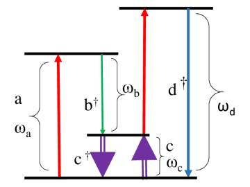
Figure 1: (Color online) Two-photon stimulated Raman scheme. The pump photon is converted into a Stokes photon and a phonon. The pump photon can also mix with a phonon to produce an anti-Stokes photon.

Remaining part of the present paper is organized as follows. In Section II, the Hamiltonian of stimulated Raman processes and its operator solution are briefly described. In Section III, the solution is used to show the existence of higher order two-mode, three-mode, and four-mode entanglement and the effect of phase of the pump mode on the higher order entanglement. Finally, the paper is concluded in Section IV.

II Model Hamiltonian

A completely quantum mechanical description of stimulated and spontaneous Raman processes described in Fig. 1 is given by the Hamiltonian szlachetka1 ; szlachetka2 ; raman-pra ; walls ; bsen1 ; bsen2 ; bsen3 ; bsen4

$$\begin{array}[]{lcl}H&=&\omega_{a}a^{\dagger}a+\omega_{b}b^{\dagger}b+\omega_{c}c^{\dagger}c+\omega_{d}d^{\dagger}d\\ &+&g\left(ab^{\dagger}c^{\dagger}+h.c.\right)+\chi\left(acd^{\dagger}+\mathrm{h.c.}\right),\end{array}$$ (1)

where h.c. stands for the Hermitian conjugate. Throughout the present paper, we use $\hbar=1$. The annihilation (creation) operators $a(a^{\dagger}),\,b(b^{\dagger}),\,c\left(c^{\dagger}\right),\,d(d^{\dagger})$ correspond to the laser (pump) mode, Stokes mode, vibration (phonon) mode and anti-Stokes mode, respectively. They obey the well-known bosonic commutation relations. The frequencies $\omega_{a}$, $\omega_{b}$, $\omega_{c}$ and $\omega_{d}$ correspond to the frequencies of pump mode $a$, Stokes mode $b$, vibration (phonon) mode $c$ and anti-Stokes mode $d$, respectively. The parameters $g$ and $\chi$ are the Stokes and anti-Stokes coupling constants, respectively. Coupling constant $g$ ($\chi$) denotes the strength of coupling between the Stokes (anti-Stokes) mode and the vibrational (phonon) mode and depends on the actual interaction mechanism. The dimension of $g$ and $\chi$ are that of frequency and consequently $gt$ and $\chi t$ are dimensionless. Further, $gt$ and $\chi t$ are very small compared to unity. Further, we would like to note that in our present study, only one vibration (phonon) mode has been considered for the mathematical simplicity. In order to study the possibility of the existence of higher order entanglement, we need simultaneous solutions of the following Heisenberg operator equations of motion for various field operators:

$$\begin{array}[]{lcl}\dot{a}&=&-i\left(\omega_{a}a+gbc+\chi cd\right)\\ \dot{b}&=&-i\left(\omega_{b}b+gac^{\dagger}\right)\\ \dot{c}&=&-i\left(\omega_{c}c+gab^{\dagger}+\chi a^{\dagger}d\right)\\ \dot{d}&=&-i\left(\omega_{d}d+\chi ac\right).\end{array}$$ (2)

The above set of equations (2) is coupled nonlinear differential equations of filed operator and are not exactly solvable in the closed analytical form under weak pump condition. However, for the very strong pump, the operator $a$ can be replaced by a $c$ number and these equations (2) are exactly solvable in that case perina . In order to solve these equations under weak pump approximation, we have used Sen-Mandal perturbative approach bsen1 ; bsen2 ; bsen3 ; bsen4 . The solutions obtained using this approach are more general than the one obtained for the same system using well-known short-time approximation. Details of the calculations are given in our previous papers bsen1 ; bsen2 ; bsen3 ; bsen4 . Here we just note that under weak pump approximation, the solutions of Eq. (2) assume the following form:

$$\begin{array}[]{lcl}a(t)&=&f_{1}a(0)+f_{2}b(0)c(0)+f_{3}c^{\dagger}(0)d(0)+f_{4}a^{\dagger}(0)b(0)d(0)+f_{5}a(0)b(0)b^{\dagger}(0)\\ &+&f_{6}a(0)c^{\dagger}(0)c(0)+f_{7}a(0)c^{\dagger}(0)c(0)+f_{8}a(0)d^{\dagger}(0)d(0),\\ b(t)&=&g_{1}b(0)+g_{2}a(0)c^{\dagger}(0)+g_{3}a^{2}(0)d^{\dagger}(0)+g_{4}c^{\dagger^{2}}(0)d(0)+g_{5}b(0)c(0)c^{\dagger}(0)\\ &+&g_{6}b(0)a(0)a^{\dagger}(0),\\ c(t)&=&h_{1}c(0)+h_{2}a(0)b^{\dagger}(0)+h_{3}a^{\dagger}(0)d(0)+h_{4}b^{\dagger}(0)c^{\dagger}(0)d(0)+h_{5}c(0)a(0)a^{\dagger}(0)\\ &+&h_{6}c(0)b(0)b^{\dagger}(0)+h_{7}c(0)d^{\dagger}(0)d(0)+h_{8}c(0)a^{\dagger}(0)a(0),\\ d(t)&=&l_{1}d(0)+l_{2}a(0)c(0)+l_{3}a^{2}(0)b^{\dagger}(0)+l_{4}b(0)c^{2}(0)+l_{5}c^{\dagger}(0)c(0)d(0)\\ &+&l_{6}a(0)a^{\dagger}(0)d(0).\end{array}.$$ (3)

The parameters $f_{i},\,g_{i},\,h_{i}$ and $l_{i}$ are computed the initial boundary conditions. In order to obtain the solutions we use the boundary condition as at $t=0$, in the first term of the Eq. (3). It is clear that $f_{1}(0)=g_{1}(0)=h_{1}(0)=l_{1}(0)=1$ and $f_{i}(0)=g_{i}(0)=h_{i}(0)=l_{i}(0)=0$ (for $i=2,\,3,\,4,\,5,\,6,\,7$ and $8$). Under these initial conditions the corresponding solutions for $f_{i}(t),\,g_{i}(t),\,h_{i}(t)$ and $l_{i}(t)$ are already reported in our earlier work bsen1 ; bsen2 ; bsen3 ; bsen4 . The same is included here as Appendix A.

The solution (3), is valid up to the second orders in $g$ and $\chi$. In what follows, we consider $\Delta\omega_{1}=\omega_{b}+\omega_{c}-\omega_{a}$ and $\Delta\omega_{2}=\omega_{a}+\omega_{c}-\omega_{d}$. The detunings $\Delta\omega_{1}$ and $\Delta\omega_{2}$ are usually very small. In the present work we have chosen $|\Delta\omega_{1}|=0.1$ MHz and $|\Delta\omega_{2}|=0.19$ MHz.

III Higher order intermodal entanglement

In order to investigate the higher-order entanglement in spontaneous and stimulated Raman processes, we assume that all photon and phonon modes are initially coherent. In other words, the composite boson field consisting of photons and phonon is in an initial state which is product of coherent states. Therefore, the composite coherent state arises from the product of the coherent states $|\alpha_{1}\rangle,\,|\alpha_{2}\rangle$, $|\alpha_{3}\rangle,$ and $|\alpha_{4}\rangle$ which are the eigenkets of $a,\,b,\,c$ and $d$ respectively. Thus, the initial composite state is

$$|\psi(0)\rangle=|\alpha_{1}\rangle\otimes|\alpha_{2}\rangle\otimes|\alpha_{3}\rangle\otimes|\alpha_{4}\rangle.$$ (4)

It is clear that the initial state is separable. Now the field operator $a(0)$ operating on such a composite coherent state gives rise to the complex eigenvalue $\alpha_{1}.$ Hence we have,

$$a(0)|\psi(0)\rangle=\alpha_{1}|\psi(0)\rangle,$$ (5)

where $|\alpha_{1}|^{2}$ is the number of input photons in the pump mode. In a similar fashion, we can also describe three more complex amplitudes $\alpha_{2}(t)$, $\alpha_{3}(t)$ and $\alpha_{4}(t)$ corresponding to the Stokes, vibrational (phonon) and anti-Stokes field mode operators $b,$ $c$ and $d$, respectively. It is clear that for a spontaneous process, the complex amplitudes except for the pump mode, are necessarily zero. Thus, in the spontaneous Raman process, $\alpha_{2}=\alpha_{3}=\alpha_{4}=0$ and $\alpha_{1}\neq 0.$ For partially spontaneous process Anirban with Perina , the complex amplitude $\alpha_{1}$ and any one/two of the remaining three eigenvalues are nonzero while the other two/one complex amplitudes are/is zero. In the present investigation, we consider that the eigenvalue corresponding to the pump mode is complex i.e., $\alpha_{1}=\left|\alpha_{1}\right|e^{-i\phi}$, where $\phi$ is the phase angle, but the other eigenvalues (i.e., eigenvalues for the Stokes, vibrational (phonon) and anti-Stokes modes) are real.

III.1 Higher order two mode entanglement

In order to investigate the higher order two mode entanglement, we use two criteria due to Hillery and Zubairy hz-prl ; two-mode-citeria-hz . The first criteria of Hillery and Zubairy is

$$E_{i,j}^{n,m}=\langle i^{\dagger n}i^{n}j^{\dagger m}j^{m}\rangle-|\langle i^{n}j^{\dagger m}\rangle|^{2}<0,$$ (6)

and the second criterion is

$$E_{i,j}^{\prime n,m}=\langle i^{\dagger n}i^{n}\rangle\langle j^{\dagger m}j^{m}\rangle-|\langle i^{n}j^{m}\rangle|^{2}<0.$$ (7)

where$i$ and $j$ are any two arbitrary operators and $i,j\in\{a,b,c,d\}\forall i\neq j.$ Here $m$ and $n$ are the positive integers and the lowest possible values of $m$ and $n$ are $m=n=1,$ which corresponds to the normal (lowest) order intermodal entanglement. A quantum state is said to be higher order entangled (bi-partite) if it is found to satisfy the equation (6) and/or equation (7) for any choice of the integers $m$ and $n$ satisfying $m+n\geq 3.$ From here onward we will refer to these criteria (6) and (7) as HZ-1 criterion and HZ-2 criterion, respectively. More specifically, a higher order entangled state is one which is witnessed via a higher order (order $k>2)$ correlation function and as per this definition all multi-partite (multi-mode) entangled states are also higher order entangled.

Before we proceed further, we note that these two criteria are only sufficient (not necessary) for detection of entanglement. Keeping this fact in mind, we have applied both of these two criteria to investigate the existence of higher order intermodal entanglement between various modes and have observed higher order intermodal entanglement in various situations. In what follows, we have also investigated the possibility of observing 3-mode and 4-mode entanglement.

Let us first investigate the possibility of two mode entanglement in Raman process using HZ-1 and HZ-2 criteria. From Eqs. (3), (4), (6) and (7), we obtain the expression for the intermodal entanglement in pump and Stokes mode as

$$\begin{array}[]{lcl}\left(\begin{array}[]{c}E_{a,b}^{n,m}\\ E_{a,b}^{\prime n,m}\end{array}\right)&=&\left|f_{2}\right|^{2}m\left(m\left|\alpha_{1}\right|^{2\left(n+1\right)}\left|\alpha_{2}\right|^{2\left(m-1\right)}\mp n\left|\alpha_{1}\right|^{2n}\left|\alpha_{2}\right|^{2m}\right)+\left|f_{3}\right|^{2}n^{2}\left|\alpha_{1}\right|^{2\left(n-1\right)}\left|\alpha_{2}\right|^{2m}\left|\alpha_{4}\right|^{2}\end{array}.$$ (8)

In the similar manner, for the remaining cases, we obtain expressions for $E_{i,j}^{n,m}$ and $E_{i,j}^{\prime n,m}:i,j\in\{a,b,c,d\}\forall i\neq j$ using HZ-1 and HZ-2 criteria as follows

$$\begin{array}[]{lcl}\left(\begin{array}[]{c}E_{b,c}^{n,m}\\ E_{b,c}^{\prime nm,}\end{array}\right)&=&\left|g_{2}\right|^{2}\left|\alpha_{2}\right|^{2\left(n-1\right)}\left|\alpha_{3}\right|^{2\left(m-1\right)}\left\{n^{2}\left(1\pm 2m\right)\left|\alpha_{1}\right|^{2}\left|\alpha_{3}\right|^{2}+m^{2}\left(1\pm 2n\right)\left|\alpha_{1}\right|^{2}\left|\alpha_{2}\right|^{2}\right.\\ &\pm&\left.m^{2}n^{2}\left|\alpha_{1}\right|^{2}\mp mn\left|\alpha_{2}\right|^{2}\left|\alpha_{3}\right|^{2}\right\}+\left|h_{3}\right|^{2}m^{2}\left|\alpha_{2}\right|^{2n}\left|\alpha_{3}\right|^{2\left(m-1\right)}\left|\alpha_{4}\right|^{2}\\ &\pm&\left[g_{1}g_{2}^{\star}mn\left|\alpha_{2}\right|^{2\left(n-1\right)}\left|\alpha_{3}\right|^{2\left(m-1\right)}\alpha_{1}^{\star}\alpha_{2}\alpha_{3}+g_{1}^{2}g_{2}^{\star 2}mn\left|\alpha_{2}\right|^{2\left(n-2\right)}\left|\alpha_{3}\right|^{2\left(m-2\right)}\right.\\ &\times&\alpha_{1}^{\star 2}\alpha_{2}^{2}\alpha_{3}^{2}\left\{\frac{1}{2}\left(m-1\right)\left(n-1\right)+\left(m-1\right)\left|\alpha_{2}\right|^{2}+\left(n-1\right)\left|\alpha_{3}\right|^{2}\right\}+h_{2}h_{3}^{\star}m^{2}n\alpha_{1}^{2}\alpha_{2}^{\star}\alpha_{4}^{\star}\\ &\times&\left|\alpha_{2}\right|^{2\left(n-1\right)}\left|\alpha_{3}\right|^{2\left(m-1\right)}+g_{1}g_{4}^{\star}mn\left|\alpha_{2}\right|^{2\left(n-1\right)}\left|\alpha_{3}\right|^{2\left(m-2\right)}\alpha_{2}\alpha_{3}^{2}\alpha_{4}^{\star}\left(2\left|\alpha_{3}\right|^{2}+m-1\right)\\ &+&\left.h_{1}^{\star 2}h_{2}h_{3}mn\left(m-1\right)\left|\alpha_{1}\right|^{2}\left|\alpha_{2}\right|^{2\left(n-1\right)}\left|\alpha_{3}\right|^{2\left(m-2\right)}\alpha_{2}^{\star}\alpha_{3}^{\star 2}\alpha_{4}+{\rm c.c.}\right].\end{array}$$ (9)

$$\begin{array}[]{lcl}\left(\begin{array}[]{c}E_{a,c}^{n,m}\\ E_{a,c}^{\prime n,m}\end{array}\right)&=&\left|f_{2}\right|^{2}m\left|\alpha_{1}\right|^{2n}\left|\alpha_{3}\right|^{2\left(m-1\right)}\left(m\left|\alpha_{1}\right|^{2}\mp n\left|\alpha_{3}\right|^{2}\right)\\ &+&\left|f_{3}\right|^{2}\left|\alpha_{1}\right|^{2\left(n-1\right)}\left|\alpha_{3}\right|^{2\left(m-1\right)}\left\{m^{2}\left(1\pm 2n\right)\left|\alpha_{1}\right|^{2}\left|\alpha_{4}\right|^{2}+n^{2}\left(1\pm 2m\right)\left|\alpha_{3}\right|^{2}\left|\alpha_{4}\right|^{2}\right.\\ &\mp&\left.mn\left|\alpha_{1}\right|^{2}\left|\alpha_{3}\right|^{2}+m^{2}n^{2}\left|\alpha_{4}\right|^{2}\right\}\pm\left[f_{1}f_{3}^{\star}mn\left|\alpha_{1}\right|^{2\left(n-1\right)}\alpha_{1}\left|\alpha_{3}\right|^{2\left(m-1\right)}\alpha_{3}\alpha_{4}^{\star}\right.\\ &+&h_{2}^{\star}h_{3}m^{2}n\alpha_{1}^{\star 2}\left|\alpha_{1}\right|^{2\left(n-1\right)}\alpha_{2}\left|\alpha_{3}\right|^{2\left(m-1\right)}\alpha_{4}+f_{2}f_{3}^{\star}mn^{2}\left|\alpha_{1}\right|^{2\left(n-1\right)}\alpha_{2}\left|\alpha_{3}\right|^{2\left(m-1\right)}\alpha_{3}^{2}\alpha_{4}^{\star}\\ &+&f_{1}^{\star 2}f_{3}^{2}mn\alpha_{1}^{\star 2}\left|\alpha_{1}\right|^{2\left(n-2\right)}\alpha_{3}^{\star 2}\left|\alpha_{3}\right|^{2\left(m-2\right)}\alpha_{4}^{2}\left\{\left(n-1\right)\left|\alpha_{3}\right|^{2}+\left(m-1\right)\left|\alpha_{1}\right|^{2}+\frac{\left(m-1\right)\left(n-1\right)}{2}\right\}\\ &+&f_{1}^{\star}f_{2}h_{1}^{\star}h_{3}mn\left(n-1\right)\alpha_{1}^{\star 2}\left|\alpha_{1}\right|^{2\left(n-2\right)}\alpha_{2}\left|\alpha_{3}\right|^{2m}\alpha_{4}\\ &+&\left.f_{1}f_{3}^{\star}h_{1}h_{2}^{\star}mn\left(m-1\right)\left|\alpha_{1}\right|^{2n}\alpha_{2}\left|\alpha_{3}\right|^{2\left(m-2\right)}\alpha_{3}^{2}\alpha_{4}^{\star}+c.c.\right]\end{array}$$ (10)

$$\begin{array}[]{lcl}\left(\begin{array}[]{c}E_{a,d}^{n,m}\\ E_{a,d}^{\prime n,m}\end{array}\right)&=&\left|f_{3}\right|^{2}n\left|\alpha_{1}\right|^{2\left(n-1\right)}\left|\alpha_{4}\right|^{2m}\left(n\left|\alpha_{4}\right|^{2}\mp m\left|\alpha_{1}\right|^{2}\right)\end{array}$$ (11)

$$\begin{array}[]{lcl}\left(\begin{array}[]{c}E_{c,d}^{n,m}\\ E_{c,d}^{\prime n,m}\end{array}\right)&=&\left|h_{2}\right|^{2}n^{2}\left|\alpha_{1}\right|^{2}\left|\alpha_{3}\right|^{2\left(n-1\right)}\left|\alpha_{4}\right|^{2m}+\left|l_{2}\right|^{2}\left|\alpha_{3}\right|^{2\left(n-1\right)}\left|\alpha_{4}\right|^{2m}\left[n^{2}\left|\alpha_{4}\right|^{2}\mp mn\left|\alpha_{3}\right|^{2}\right]\end{array}$$ (12)

$$\begin{array}[]{lcl}\left(\begin{array}[]{c}E_{bd}^{n,m}\\ E_{b,d}^{\prime n,m}\end{array}\right)&=&\left|g_{2}\right|^{2}n^{2}\left|\alpha_{1}\right|^{2}\left|\alpha_{2}\right|^{2\left(n-1\right)}\left|\alpha_{4}\right|^{2m}\pm\left[l_{1}^{\star}l_{3}mn\alpha_{1}^{2}\alpha_{2}^{\star}\left|\alpha_{2}\right|^{2\left(n-1\right)}\alpha_{4}^{\star}\left|\alpha_{4}\right|^{2\left(m-1\right)}+c.c.\right]\end{array}$$ (13)

Here we would like to note that once we obtain analytic expressions for $E_{i,j}^{n,m}$ and $E_{i,j}^{\prime n,m}$ in stimulated Raman process, it is straightforward to study the special cases: (i) spontaneous Raman process, where $\alpha_{2}=\alpha_{3}=\alpha_{4}=0,$ but $\alpha_{1}\neq 0,$ and (ii) partially spontaneous Raman process, where $\alpha_{1}\neq 0$ and any one/two of the other three $\alpha_{i}\,(i=2,\,3,\,4)$ is/are non-zero. It is clear from the Eqs. (8-13) that for spontaneous Raman process Eqs. (8-13) reduces to zero. Hence for the spontaneous Raman process, no signature of intermodal entanglement is observed. To investigate the possibility of higher order intermodal entanglement in the stimulated Raman process we have used $\chi=g=10^{4}$ Hz, $|\alpha_{1}|=10,$ $|\alpha_{2}|=8,$ $|\alpha_{3}|=0.01,$ $|\alpha_{4}|=1$ foot2 . We have plotted the right hand side of (8 -13) in Fig. 2 and Fig. 3 for $m=1$and $n=1,\,2$ and $3.$We observed that HZ-1 criteria can detect the higher order intermodal entanglement in the stimulated Raman process for different values of the phase angle or all phase angles of the input pump field (i.e., for $\phi=0,\,\frac{\pi}{2}$ and $\pi$) for all the possible modes except pump-phonon ($ac$) and phonon-anti-Stokes ($cd$ ) modes. It is interesting to note that higher order intermodal entanglement is observed in pump-Stokes mode, although in the lowest order it was not observed. Further, the figures show that the depths of the nonclassicality parameters $E_{i,j}^{n,m}$ and $E_{i,j}^{\prime n,m}$ increase with the order. Use of HZ-1 criteria also led to similar features in the partially spontaneous Raman process (not in figure). In other words, we observed signatures of intermodal entanglement in all the cases except pump-phonon ($ac$) and phonon-anti-Stokes ($cd$) modes. As HZ-1 is only a sufficient (not necessary) criterion, it may have failed to witness entanglement, keeping this fact in mind, we have plotted the right hand side of Eq. (8- 13) using HZ-2 criteria (See Fig. 3). It is interesting to note that HZ-2 criterion can detect the higher order intermodal entanglement in pump-phonon ($ac$) mode for phase angle $\phi=\frac{\pi}{2}$, which was not detected by HZ-1 criterion, in the stimulated and partial spontaneous Raman processes. However, we do not observe any signature of higher order intermodal entanglement for spontaneous Raman process. Thus, the stimulated Raman process provides a very nice example of a physical system which can produce higher order entanglement.

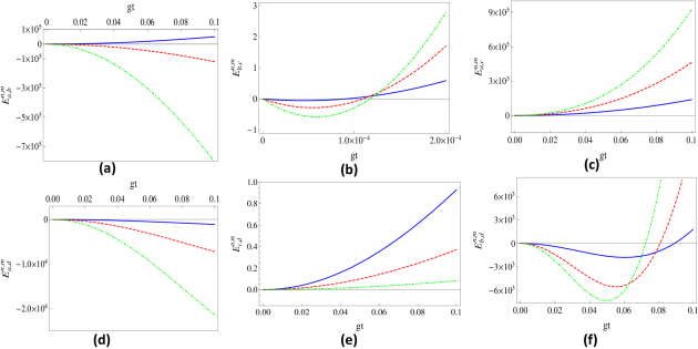
Figure 2: (Colour online) Higher order intermodal entanglement in stimulated Raman process with $\left|\alpha_{1}\right|=10,$ $\left|\alpha_{2}\right|=8,$ $\left|\alpha_{3}\right|=0.01$ and $\left|\alpha_{4}\right|=1$ using HZ-1 criteron is shown for diffrent values of phase angle ($\phi=0,$ $\frac{\pi}{2}$ and $\pi$) in pump mode. Higher order intermodal entanglement is observed in (a) pump-Stokes mode for phase angle $0,$ (b) Stokes-vibration phonon mode for phase angle $\phi=\frac{\pi}{2},$ (d) pump-anti-Stokes mode for phase angle $0,$ (f) Stokes-anti-Stokes mode for phase angle $0$; and not observed in (c) pump-vibration phonon mode and (e) vibration phonon-anti-Stokes mode. In all the plots, the smooth line, dotted line and dash-dotted line are used for the $m=1$ and $n=1,$ $2$ and $3$, respectively. In (e), $n=2$ and 3 are multiplied by $10^{3}$ and $10^{6}$, respectively. While in all the remaining cases, $n=1$ and 2 are shown 1500 and 50 times, respectively.

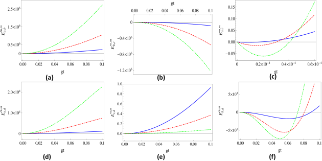
Figure 3: (Colour online) Higher order intermodal entanglement in stimulated Raman process is illustrated using HZ-2 criterion with different phase angle ($\phi=0,$ $\frac{\pi}{2}$ and $\pi$) in pump mode for $\left|\alpha_{1}\right|=10,$ $\left|\alpha_{2}\right|=8,$ $\left|\alpha_{3}\right|=0.01$ and $\left|\alpha_{4}\right|=1$. Specifically, higher order intermodal entanglement is observed in (b) for Stokes-vibration phonon mode with phase angle $\phi=\frac{\pi}{2},$ (c) for pump-vibration phonon mode with phase angle $\phi=\frac{\pi}{2},$ and (f) for Stokes-anti-Stokes mode with phase angle $\frac{\pi}{2}$. However, in (a), (d) and (e) higher order intermodal entanglement is not observed for pump-Stokes, pump-anti-Stokes and vibration phonon-anti-Stokes modes, respectively. The smooth, dotted and dash-dotted lines are used for $m=1$ and $n=1,$ $2$ and $3$, respectively. Here, for (e) $n=2$ and 3 are multiplied by $10^{3}$ and $10^{6}$, respectively. For all the remaining cases, $n=1$ and 2 are shown 1500 and 50 times, respectively.

III.2 Three mode entanglement

There exists another alternative way to study the higher-order entanglement. To be precise, all multi-mode entanglements are essentially higher-order entanglement. In other words, three mode entanglement always indicates higher order entanglement. In order to investigate the three mode entanglement, we use the following criterion Ent condition-multimode

$$E_{a,b,c}^{\prime}=\begin{array}[]{lcl}\begin{array}[]{lcl}\left\langle N_{a}\right\rangle\left\langle N_{b}\right\rangle\left\langle N_{c}\right\rangle&-&\left|\left\langle abc\right\rangle\right|^{2}\end{array}&<&0\end{array},$$ (14)

where $\left\langle N_{a}\right\rangle,$ $\left\langle N_{b}\right\rangle,$ and $\left\langle N_{c}\right\rangle$ are average value of the number operators of the pump mode Stokes mode and vibration phonon mode respectively. Using equations (3), (4) and (14) we obtain

$$\begin{array}[]{lcl}E_{a,b,c}^{\prime}&=&\left\langle N_{a}\right\rangle\left\langle N_{b}\right\rangle\left\langle N_{c}\right\rangle-\left|\left\langle abc\right\rangle\right|^{2}\\ &=&\left|f_{2}\right|^{2}\left(5\left|\alpha_{1}\right|^{2}\left|\alpha_{2}\right|^{2}\left|\alpha_{3}\right|^{2}-\left|\alpha_{1}\right|^{4}\left|\alpha_{3}\right|^{2}-\left|\alpha_{1}\right|^{4}-\left|\alpha_{1}\right|^{4}\left|\alpha_{2}\right|^{2}\right)\\ &+&\left|f_{3}\right|^{2}\left(\left|\alpha_{1}\right|^{2}\left|\alpha_{2}\right|^{2}\left|\alpha_{3}\right|^{2}-4\left|\alpha_{2}\right|^{2}\left|\alpha_{4}\right|^{2}-3\left|\alpha_{2}\right|^{2}\left|\alpha_{3}\right|^{2}\left|\alpha_{4}\right|^{2}-3\left|\alpha_{1}\right|^{2}\left|\alpha_{2}\right|^{2}\left|\alpha_{4}\right|^{2}\right)+\\ &-&\left[h_{1}h_{2}^{\star}\alpha_{1}^{\star}\left|\alpha_{1}\right|^{2}\alpha_{2}\alpha_{3}+2f_{1}f_{3}^{\star}\alpha_{1}\left|\alpha_{2}\right|^{2}\alpha_{3}\alpha_{4}^{\star}+h_{2}h_{3}^{\star}\left(2\alpha_{1}^{2}\alpha_{2}^{\star}\alpha_{4}^{\star}\right.\right.\\ &+&\left.\left.\left|\alpha_{1}\right|^{2}\alpha_{1}^{2}\alpha_{2}^{\star}\alpha_{4}^{\star}+2\alpha_{1}^{2}\alpha_{2}^{\star}\left|\alpha_{2}\right|^{2}\alpha_{4}^{\star}\right)+{\rm c.c.}\right].\end{array}$$ (15)

For the spontaneous Raman process, Eq. (15) reduces to

$$\begin{array}[]{lcl}E_{a,b,c}^{\prime}&=&-\left|f_{2}\right|^{2}\left|\alpha_{1}\right|^{4}\end{array},$$ (16)

which is clearly negative and thus indicate the existence of tripartite entanglement in the spontaneous Raman process.

To investigate the existence of three mode entanglement in the stimulated Raman process, we plot the right hand side of the equation (15) in Fig.4 for three different values of the phase angle of the input pump field, i.e., for $\phi=0$ (blue smooth line), $\phi=\frac{\pi}{2}$ (red dotted line) and $\phi=\pi$ (green dash dotted line). The negative regions of the plots clearly illustrate the existence of tri-modal (higher order) entanglement. From Fig.4

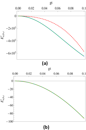
Figure 4: (Colour online) The variation of three mode entanglement among pump, Stokes and vibration phonon modes (a) for stimulated Raman process using $\left|\alpha_{1}\right|=10,$ $\left|\alpha_{2}\right|=8,$ $\left|\alpha_{3}\right|=0.01$, $\left|\alpha_{4}\right|=1$ (b) for spontaneous Raman process using $\left|\alpha_{1}\right|=10,$ $\left|\alpha_{2}\right|=\left|\alpha_{3}\right|=\left|\alpha_{4}\right|=0$ with the smooth, dashed and dash-dotted lines corresponding to $\phi=0,$ $\frac{\pi}{2}$ and $\pi,$ respectively.

we can clearly observe the signature of higher order entanglement for different values of phase angle of the input pump field for stimulated and spontaneous Raman processes.

III.3 Four mode entanglement

In order to investigate the four mode entanglement we use the following criterion, which is similar to that of Li et al.’s three mode criterion Ent condition-multimode :

$$\begin{array}[]{lcl}E_{a,b,c,d}^{\prime}&=&\left\langle N_{a}\right\rangle\left\langle N_{b}\right\rangle\left\langle N_{c}\right\rangle\left\langle N_{d}\right\rangle-\left|\left\langle abcd\right\rangle\right|^{2}<0,\end{array}$$ (17)

where $a,$$b,$$c$ and $d$ are arbitrary operators and the negative value of $E_{a,b,c,d}^{\prime}$ gives the signature of the higher order entanglement. Now, we investigate the higher order entanglement i.e., the entanglement among the four modes of the stimulated Raman and spontaneous Raman processes and we obtain

$$\begin{array}[]{lcl}E_{a,b,c,d}^{\prime}&=&\left|f_{2}\right|^{2}\left|\alpha_{1}\right|^{2}\left(5\left|\alpha_{2}\right|^{2}\left|\alpha_{3}\right|^{2}\left|\alpha_{4}\right|^{2}-\left|\alpha_{1}\right|^{2}\left|\alpha_{3}\right|^{2}\left|\alpha_{4}\right|^{2}-\left|\alpha_{1}\right|^{2}\left|\alpha_{4}\right|^{2}\right)\\ &+&\left|f_{3}\right|^{2}\left|\alpha_{2}\right|^{2}\left|\alpha_{4}\right|^{2}\left(7\left|\alpha_{1}\right|^{2}\left|\alpha_{3}\right|^{2}-4\left|\alpha_{4}\right|^{2}-3\left|\alpha_{1}\right|^{2}\left|\alpha_{4}\right|^{2}-3\left|\alpha_{3}\right|^{2}\left|\alpha_{4}\right|^{2}\right)\\ &-&\left[h_{1}^{\star}h_{2}\left|\alpha_{1}\right|^{2}\alpha_{1}\alpha_{2}^{\star}\alpha_{3}^{\star}\left|\alpha_{4}\right|^{2}+2f_{1}^{\star}f_{3}\alpha_{1}^{\star}\left|\alpha_{2}\right|^{2}\alpha_{3}^{\star}\left|\alpha_{4}\right|^{2}\alpha_{4}+f_{2}f_{3}^{\star}\left|\alpha_{2}\right|^{2}\alpha_{2}\alpha_{3}^{2}\alpha_{4}^{\star}\left|\alpha_{4}\right|^{2}\right.\\ &+&\left(l_{1}^{\star}l_{3}-h_{2}h_{3}^{\star}\right)\left|\alpha_{1}\right|^{2}\alpha_{1}^{2}\alpha_{2}^{\star}\left|\alpha_{3}\right|^{2}\alpha_{4}^{\star}+h_{2}h_{3}^{\star}\left(2\alpha_{1}^{2}\alpha_{2}^{\star}\alpha_{4}^{\star}\left|\alpha_{4}\right|^{2}+\left|\alpha_{1}\right|^{2}\alpha_{1}^{2}\alpha_{2}^{\star}\alpha_{4}^{\star}\left|\alpha_{4}\right|^{2}\right.\\ &+&\left.2\alpha_{1}^{2}\alpha_{2}^{\star}\left|\alpha_{2}\right|^{2}\alpha_{4}^{\star}\left|\alpha_{4}\right|^{2}+3\alpha_{1}^{2}\alpha_{2}^{\star}\left|\alpha_{3}\right|^{2}\alpha_{4}^{\star}\left|\alpha_{4}\right|^{2}\right)+f_{1}f_{2}^{\star}h_{1}^{\star}h_{2}\alpha_{1}^{2}\alpha_{2}^{\star 2}\alpha_{3}^{\star 2}\left|\alpha_{4}\right|^{2}\\ &+&h_{1}^{\star}h_{2}l_{1}l_{2}^{\star}\left(\left|\alpha_{1}\right|^{4}\alpha_{2}^{\star}\alpha_{3}^{\star 2}\alpha_{4}+\alpha_{2}^{\star}\left|\alpha_{2}\right|^{2}\alpha_{3}^{\star 2}\left|\alpha_{4}\right|^{2}\alpha_{4}\right)+2f_{1}^{\star}f_{3}l_{1}l_{2}^{\star}\alpha_{1}^{\star 2}\left|\alpha_{2}\right|^{2}\alpha_{3}^{\star 2}\alpha_{4}^{2}\\ &+&\left.\left(h_{1}^{\star}h_{4}+3g_{1}^{\star}g_{2}h_{1}^{\star}h_{3}\right)\left|\alpha_{1}\right|^{2}\alpha_{2}^{\star}\alpha_{3}^{\star 2}\left|\alpha_{4}\right|^{2}\alpha_{4}+c.c.\right]\end{array}$$ (18)

In order to investigate the possibility of observing 4-mode entanglement in the Raman processes, in Fig. 5, we have plotted the variation of right hand side of Eq. (18) with the rescaled time $gt$. Quite interestingly, for appropriate choice of the phase of the pump mode, 4 mode entanglement is observed in both stimulated Raman process and partially spontaneous Raman process.

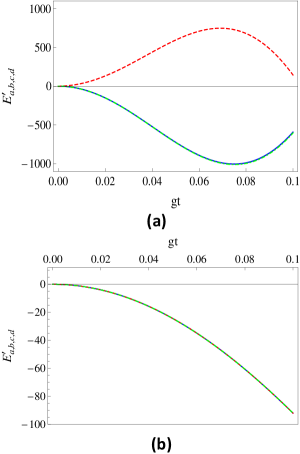
Figure 5: (Colour online) Four mode entanglement among pump, Stokes, vibration phonon and anti-Stokes modes is depicted in (a) stimulated Raman process using $\left|\alpha_{1}\right|=10,$ $\left|\alpha_{2}\right|=8,$ $\left|\alpha_{3}\right|=0.01$, $\left|\alpha_{4}\right|=1$ (b) partial spontaneous Raman process using $\left|\alpha_{1}\right|=10,$ $\left|\alpha_{2}\right|=\left|\alpha_{3}\right|=0$. Here, the smooth line, dashed line and dash-dotted line corresponds to $\phi=0,$ $\frac{\pi}{2}$ and $\pi,$ respectively.

IV Conclusions

Recently, nonclassical properties of the stimulated Raman process have been extensively studied by some of the present authors Anirban with Perina ; raman-pra . In those studies intermodal entanglement in different modes of the stimulated Raman process was reported. Intermodal entanglement between Stokes mode and the vibration mode in the Raman processes was also reported by Kuznetsov kuznetsov . However, higher order entanglement was not investigated. In the present paper higher order entanglement in stimulated Raman process is studied in detail and the observed higher order entanglement are illustrated through the negative regions of the Figs.2-5. In Figs. 2 and 3, the existence of higher order two-mode entanglement between various possible combinations of modes are illustrated using HZ-1 criterion and HZ-2 criterion, respectively. Specifically, using HZ-1 criterion, we have observed the intermodal higher order entanglement for all the possible combinations of modes, except pump-phonon $(ac)$ and phonon-anti-Stokes $(cd)$ modes in stimulated Raman process (cf. Fig.2) and in partially spontaneous Raman processes (not shown in figure). However, we found that HZ-2 criteria can detect the signature of higher order intermodal entanglement only in Stokes-phonon ($bc$), pump-phonon ($ac$) and Stokes-anti-Stokes ($bd$) modes in the stimulated and partially spontaneous Raman process Fig.3, but it is interesting to note that HZ-2 criteria can detect the higher order intermodal entanglement in pump-phonon ($ac$) mode whereas HZ-1 criteria fails to detect this. Thus, by combining the results, we have observed the existence of two-mode higher order entanglement in stimulated and partially spontaneous Raman possesses in all possible cases except in phonon-anti-Stokes $(cd)$ modes. However, no signature of intermodal entanglement is observed for the spontaneous Raman process. Another interesting point is that the present investigation reveals the signature of higher order intermodal entanglement in pump-Stokes mode ($ab$) in stimulated Raman process, but intermodal entanglement in $ab$ modes were not observed in lowest order (cf. Fig. 2a, 3a and 4a of Ref. raman-pra ). As all the multi-partite (multi-mode) entanglement are essentially higher order entanglement, we investigated the possibility of observing three mode and four mode entanglements in Raman processes and found that tri-modal entanglement can be observed among pump, Stokes and vibration phonon mode ($abc$) in both stimulated and spontaneous Raman processes (cf. Fig.4), and it is also possible to observe entanglement among four modes (pump, Stokes, vibration phonon and anti-Stokes) in stimulated and partially spontaneous Raman processes (see Fig.5). As recently many applications of multi-partite entanglement has been proposed, we hope that the present observation on the possibility of observing multi-mode entanglement in Raman process would be of help in realizing some of the recently proposed schemes that are based on multi-partite entanglement. Further, it is easy to experimentally realize Raman process and thus the results reported here can be experimentally verified using the available technologies.

Bosonic Hamiltonians similar to the one studied here frequently appear in quantum optical, opto-mechanical and atomic systems. Thus, the methodology adopted here may also be used in those systems to study the existence of nonclassical states in normal and higher order entanglement in particular. Keeping this in mind, we conclude the present work with an expectation that this work would lead to a bunch of similar studies in other bosonic systems.

Appendix A Parameters for the solutions in Eq. (3)

$$f_{1} = \exp(-i\omega_{a}t),$$

$$f_{2} = \frac{ge^{-i\omega_{a}t}}{\Delta\omega_{1}}\left[e^{-i\Delta\omega_{1}t}-1\right],$$

$$f_{3} = -\frac{\chi e^{-i\omega_{a}t}}{\Delta\omega_{2}}\left[e^{i\Delta\omega_{2}t}-1\right],$$

$$f_{4} = \begin{array}[]{l}-\frac{\chi ge^{-i\omega_{a}t}}{\Delta\omega_{1}}\left[\frac{e^{-i(\Delta\omega_{1}-\Delta\omega_{2})t}-1}{\Delta\omega_{1}-\Delta\omega_{2}}+\frac{e^{i\Delta\omega_{2}t}}{\Delta\omega_{2}}\right]\\ -\frac{\chi ge^{-i\omega_{a}t}}{\Delta\omega_{2}}\left[\frac{e^{-i(\Delta\omega_{1}-\Delta\omega_{2})t}-1}{\Delta\omega_{1}-\Delta\omega_{2}}-\frac{e^{-i\Delta\omega_{1}t}}{\Delta\omega_{1}}\right],\end{array}$$ (21)

$$f_{5} = \frac{g^{2}e^{-i\omega_{a}t}}{\Delta\omega_{1}^{2}}\left[e^{-i\Delta\omega_{1}t}-1\right]+\frac{ig^{2}te^{-i\omega_{a}t}}{\Delta\omega_{1}},$$

$$f_{6} = f_{5},$$

$$f_{7} = \frac{\chi^{2}e^{-i\omega_{a}t}}{\Delta\omega_{2}^{2}}\left[e^{i\Delta\omega_{2}t}-1\right]-\frac{i\chi^{2}te^{-i\omega_{a}t}}{\Delta\omega_{2}},$$

$$f_{8} = -f_{7}.$$

$$g_{1} = \exp(-i\omega_{b}t),$$

$$g_{2} = -\frac{ge^{-i\omega_{b}t}}{\Delta\omega_{1}}\left[e^{i\Delta\omega_{1}t}-1\right],$$

$$g_{3} = \begin{array}[]{l}\frac{\chi ge^{-i\omega_{b}t}}{\Delta\omega_{2}(\Delta\omega_{1}-\Delta\omega_{2})}\left[e^{i(\Delta\omega_{1}-\Delta\omega_{2})t}-1\right]\\ -\frac{\chi ge^{-i\omega_{b}t}}{\Delta\omega_{2}\Delta\omega_{1}}\left[e^{i\Delta\omega_{1}t}-1\right],\end{array}$$ (24)

$$g_{4} = \begin{array}[]{l}\frac{\chi ge^{-i\omega_{b}t}}{\Delta\omega_{2}(\Delta\omega_{1}+\Delta\omega_{2})}\left[e^{i(\Delta\omega_{1}+\Delta\omega_{2})t}-1\right]\\ -\frac{\chi ge^{-i\omega_{b}t}}{\Delta\omega_{2}\Delta\omega_{1}}\left[e^{i\Delta\omega_{1}t}-1\right],\end{array}$$ (27)

$$g_{5} = \frac{g^{2}e^{-i\omega_{b}t}}{\Delta\omega_{1}^{2}}\left[e^{i\Delta\omega_{1}t}-1\right]-\frac{ig^{2}te^{-i\omega_{b}t}}{\Delta\omega_{1}},$$

$$g_{6} = -g_{5}.$$

$$h_{1} = \exp(-i\omega_{c}t)$$

$$h_{2} = -\frac{ge^{-i\omega_{c}t}}{\Delta\omega_{1}}\left[e^{i\Delta\omega_{1}t}-1\right]$$

$$h_{3} = -\frac{\chi e^{-i\omega_{c}t}}{\Delta\omega_{2}}\left[e^{i\Delta\omega_{2}t}-1\right]$$

$$h_{4} = \begin{array}[]{l}\frac{\chi ge^{-i\omega_{c}t}}{\Delta\omega_{2}}\left[\frac{e^{i(\Delta\omega_{1}+\Delta\omega_{2})t}-1}{\Delta\omega_{1}+\Delta\omega_{2}}-\frac{e^{i\Delta\omega_{1}t}}{\Delta\omega_{1}}\right]\\ -\frac{\chi ge^{-i\omega_{c}t}}{\Delta\omega_{1}}\left[\frac{e^{i(\Delta\omega_{1}+\Delta\omega_{2})t}-1}{\Delta\omega_{1}+\Delta\omega_{2}}-\frac{e^{i\Delta\omega_{2}t}}{\Delta\omega_{2}}\right]\end{array}$$ (30)

$$h_{5} = -\frac{g^{2}e^{-i\omega_{c}t}}{\Delta\omega_{1}^{2}}\left[e^{i\Delta\omega_{1}t}-1\right]+\frac{ig^{2}te^{-i\omega_{c}t}}{\Delta\omega_{1}}$$

$$h_{6} = -h_{5}$$

$$h_{7} = -\frac{\chi^{2}e^{-i\omega_{c}t}}{\Delta\omega_{2}^{2}}\left[e^{i\Delta\omega_{2}t}-1\right]+\frac{i\chi^{2}te^{-i\omega_{c}t}}{\Delta\omega_{2}}$$

$$h_{8} = \frac{\chi^{2}e^{-i\omega_{c}t}}{\Delta\omega_{2}^{2}}\left[e^{i\Delta\omega_{2}t}-1\right]-\frac{i\chi^{2}te^{-i\omega_{c}t}}{\Delta\omega_{2}}$$

$$l_{1} = \exp(-i\omega_{d}t)$$

$$l_{2} = \frac{\chi e^{-i\omega_{d}t}}{\Delta\omega_{2}}\left[e^{-i\Delta\omega_{2}t}-1\right]$$

$$l_{3} = \begin{array}[]{l}\frac{\chi ge^{-i\omega_{d}t}}{\Delta\omega_{1}(\Delta\omega_{1}-\Delta\omega_{2})}\left[e^{i(\Delta\omega_{1}-\Delta\omega_{2})t}-1\right]\\ +\frac{\chi ge^{-i\omega_{d}t}}{\Delta\omega_{2}\Delta\omega_{1}}\left[e^{-i\Delta\omega_{2}t}-1\right]\end{array}$$ (33)

$$l_{4} = \begin{array}[]{l}\frac{\chi ge^{-i\omega_{d}t}}{\Delta\omega_{1}(\Delta\omega_{1}+\Delta\omega_{2})}\left[e^{-i(\Delta\omega_{1}+\Delta\omega_{2})t}-1\right]\\ -\frac{\chi ge^{-i\omega_{d}t}}{\Delta\omega_{2}\Delta\omega_{1}}\left[e^{-i\Delta\omega_{2}t}-1\right]\end{array}$$ (36)

$$l_{5} = \frac{i\chi^{2}te^{-i\omega_{d}t}}{\Delta\omega_{2}}+\frac{\chi^{2}e^{-i\omega_{d}t}}{\Delta\omega_{2}^{2}}\left[e^{-i\Delta\omega_{2}t}-1\right]$$

$$l_{6} = l_{5}$$

References

• (1) C. H. Bennett, G. Brassard, C. Crepeau, R. Jozsa, A. Peres and W. K. Wootters, Phys. Rev. Lett. 70, 1895 (1993).
• (2) C. H. Bennett and S. J. Wiesner, Phys. Rev. Lett. 69, 2881 (1992).
• (3) C. Shukla and A. Pathak, Phys. Lett. A 377, 1337 (2013).
• (4) A. Pathak, Elements of Quantum Computation and Quantum Communication (CRC Press, Boca Raton, USA, 2013).
• (5) O. ${\rm G\ddot{u}hne}$, G. ${\rm T\acute{o}th}$, Phys. Rep. 474, 1 (2009).
• (6) A. Peres, Phys. Rev. Lett. 77, 1413 (1996).
• (7) L. M. Duan, G. Giedke, J. I. Cirac and P. Zollar, Phys. Rev. Lett. 84, 2722 (2000).
• (8) H. Hung and G. S. Agarwal, Phys. Rev. A, 49, 52 (1994).
• (9) J. Lee, M. S. Kim and H. Jeong, Phys. Rev. A, 62, 032305 (2000).
• (10) R. Simon, Phys. Rev. Lett. 84, 2726 (2000).
• (11) M. Hillery and M. S. Zubairy, Phys. Rev. Lett. 96, 050503 (2006).
• (12) M. Hillery and M. S. Zubairy, Phys. Rev. A 74, 032333 (2006).
• (13) M. Hillery, H. T. Dung and H. Zheng, Phys. Rev. A 81, 062322 (2010).
• (14) G. S. Agarwal and A. Biswas, New J. Phys. 7, 211 (2005).
• (15) C. H. Raymond Ooi, Q. Sun, M. Suhail Zubairy and M. O. Scully, Phys. Rev. A 75, 013820 (2007).
• (16) C. H. Raymond Ooi, Phys. Rev. A 76, 013809 (2007); Eyob A. Sete, and C. H. Raymond Ooi, Phys. Rev. A 85, 063819 (2012).
• (17) A. Miranowicz et al., Phys. Rev. A 82, 013824 (2010).
• (18) T.-C. Wei and P. M. Goldbart, Phys. Rev. A 68, 042307 (2003)
• (19) A. Miranowicz, M. Piani, P. Horodecki, and R. Horodecki, Phys. Rev. A, 80, 052303 (2009).
• (20) A. Miranowicz and S. Kielich, Mdoern Nonlinear Optics Part 3, Ed. M. Evans and S. Kielich, Adv. Chem. Phys. 85, 531 (Wiley, New York, 1994).
• (21) P. Szlachetka, S. Kielich, J. $\mathrm{Pe\breve{r}ina}$ and V. $\mathrm{Pe\breve{r}inov\acute{a}},$ J. Phys A: Math. Gen 12, 1921 (1979).
• (22) J. $\mathrm{Pe\breve{r}ina}$, Quantum Statistics of Linear and Nonlinear Optical Phenomena (Kluwer, Dordrecht, 1991).
• (23) A. Pathak, J. $\mathrm{K}\breve{\mathrm{r}}\mathrm{epelka}$ and J. $\mathrm{Pe\breve{r}ina}$, Phys. Lett. A 377, 2692 (2013).
• (24) B. Sen, S. K. Giri, S. Mandal, C. H. R. Ooi and A. Pathak, Phys. Rev. A 87, 022325 (2013).
• (25) P. Grangier, Nature 438, 749 (2005).
• (26) L. M. Duan, M. Lukin, J. I. Cirac and P. Zoller, Nature 414, 413 (2005).
• (27) A. Allevi, S. Olivares, and M. Bondani, Phys. Rev. A 85, 063835 (2012).
• (28) A. Allevi, S. Olivares, and M. Bondani, Int. J. Quant. Info. 8, 1241003 (2012).
• (29) M. Avenhaus, K. Laiho, M. V. Chekhova, and C. Silberhorn, Phys. Rev. Lett 104, 063602 (2010).
• (30) F. Haas, J. Volz, R. Gehr, J. Reichel, and ${\rm J.}$ ${\rm Est\grave{e}ve}$, Science 344, 180 (2014).
• (31) S. K. Giri, B. Sen, C. H. R. Ooi and A. Pathak, Phys. Rev. A 89, 033628 (2014).
• (32) K. Thapliyal, A. Pathak, B. Sen and J. $\mathrm{Pe\breve{r}ina},$ Phys. Rev. A 90, 013808 (2014).
• (33) S. K. Giri, K. Thapliyal, B. Sen, and A. Pathak, arXiv:1407.1780v1 [quant-ph]
• (34) K. Thapliyal, A. Pathak, B. Sen and J. $\mathrm{Pe\breve{r}ina}$, Phys. Lett. A 378, 3431 (2014).
• (35) B. Sen and S. Mandal, J. Mod. Opt. 52, 1789 (2005).
• (36) B. Sen, S. Mandal and J. $\mathrm{Pe\breve{r}ina}$, J. Phys. B:At. Mol. Opt. Phys. 40, 1417 (2007).
• (37) B. Sen and S. Mandal, J. Mod. Opt. 55, 1697 (2008).
• (38) B. Sen, V. $\mathrm{Pe\breve{r}inov\acute{a}},$ J. $\mathrm{Pe\breve{r}ina}$, A. $\mathrm{Luk}\mathrm{\breve{s}}$, and J. $\mathrm{K}\breve{\mathrm{r}}\mathrm{epelka}$, J. Phys. B: At. Mol. Opt. Phys. 44, 105503 (2011).
• (39) P. Szlachetka, S. Kielich, J. $\mathrm{Pe\breve{r}ina}$ and V. $\mathrm{Pe\breve{r}inov\acute{a}},$ Opt. Acta 27, 1609 (1980).
• (40) D. F. Walls, Z. Phys. 237, 224 (1970).
• (41) Same values of $\chi,$ $g$ and $|\alpha_{i}|$ are used in the entire paper (unless otherwise specified). For spontaneous and partially spontaneous Raman proceses these values of $|\alpha_{i}|$ are used for non-zero $|\alpha_{i}|$’s.
• (42) Z.-G. Li, S.-M. Fei, Z.-X. Wang and K. Wu, Phys. Rev. A 75, 012311 (2007).
• (43) S. V. Kuznetsov, O. V. Man’ko and N. V. Tcherniega, J. Opt. B: Quantum Semiclass. Opt. 5, S503 (2003).