Fractional Imputation in Survey Sampling: A Comparative Review

Abstract

Fractional imputation (FI) is a relatively new method of imputation for handling item nonresponse in survey sampling. In FI, several imputed values with their fractional weights are created for each missing item. Each fractional weight represents the conditional probability of the imputed value given the observed data, and the parameters in the conditional probabilities are often computed by an iterative method such as EM algorithm. The underlying model for FI can be fully parametric, semiparametric, or nonparametric, depending on plausibility of assumptions and the data structure.

In this paper, we give an overview of FI, introduce key ideas and methods to readers who are new to the FI literature, and highlight some new development. We also provide guidance on practical implementation of FI and valid inferential tools after imputation. We demonstrate the empirical performance of FI with respect to multiple imputation using a pseudo finite population generated from a sample in Monthly Retail Trade Survey in US Census Bureau.

and

1 INTRODUCTION

In survey sampling, it is a common practice to collect data on a large number of items. Even when a sampled unit responds to the survey, this unit may not respond to some items. In this scenario, imputation can be used to create a complete data set by filling in missing values with plausible values to facilitate data analyses. The goal of imputation is three-fold: First, by providing complete data, subsequent analyses are easy to implement and can achieve consistency among different users. Second, imputation reduces the selection bias associated with only using the respondent set, which may not necessarily represent the original sample. Third, the imputed data can incorporate extra information so that the resulting analyses are statistically efficient and coherent. Combining information from several surveys or creating synthetic data from planned missingness are cases in point (Schenker and Raghunathan 2007).

When the imputed data set is released to the public, it should meet the goal of multiple uses both for planned and unplanned parameters (Haziza, 2009). In a typical survey situation, the imputers may know some of the parameters of interest at the time of imputation, but hardly know the full set of possible parameters to be estimated from the data. Single imputation, such as hot deck imputation, regression imputation and stochastic regression imputation, replaces each of the missing data with one plausible value. Although single imputation has been widely used, one drawback is that it does not take into account of the full uncertainty of missing data and often falls short of multiple-purpose estimation. Multiple imputation (MI) has been proposed by Rubin (1976) to replace each of missing data with multiple plausible values to reflect the full uncertainty in the prediction of missing data. Several authors (Rubin 1987; Little and Rubin 2002; Schafer 1997) have promoted MI as a standard approach for general-purpose estimation under item nonresponse in survey sampling. Although the variance estimation formula of Rubin (1987) is simple and easy to apply, it is not always consistent (Fay 1992; Wang and Robins 1998; Kim et al. 2006). For using the MI variance estimation formula, the congeniality condition of Meng (1994) needs to be met, which can be restrictive for general-purpose inference. For example, Kim (2011) pointed out that a MI procedure that is congenial for mean estimation is not necessarily congenial for proportion estimation.

Fractional imputation (FI) is another effective imputation tool for general-purpose estimation with its advantage of not requiring the congeniality condition. FI was originally proposed by Kalton and Kish (1984) to reduce the variance of single imputation methods by replacing each missing value with several plausible values at differentiable probabilities reflected through fractional weights. Fay (1996), Kim and Fuller (2004), Fuller and Kim (2005), Durrant (2005), Durrant and Skinner (2006) discussed FI as a nonparametric imputation method for descriptive parameters of interest in survey sampling. Kim (2011) and Kim and Yang (2014) presented FI under fully parametric model assumptions.

More generally, FI can also serve as a computational tool for implementing the expectation step (E-step) in the EM algorithm (Wei and Tanner 1990; Kim 2011). When the conditional expectation in the E-step is not available in a closed form, parametric FI of Kim (2011) simplifies computation by drawing on the importance sampling idea. Through fractional weights, FI can reduce the burden of iterative computation, such as Markov Chain Monte Carlo, for evaluating the conditional expectation associated with missing data. Kim and Hong (2012) extended parametric FI to a more general class of incomplete data, including measurement error models.

Despite these advantages, FI in applied research has not been widely used due to lack of good information that provides researchers with comprehensive understanding of this approach. The goal of this paper is to bring more attention to FI by reviewing existing research on FI, introducing key ideas and methods, and highlighting some new development, mainly in the context of survey sampling. This paper also provides guidance on practical implementations and applications of FI.

This paper is organized as follows. Section 2 provides the basic setup and Section 3 introduces FI under parametric model assumptions. Section 4 discusses a nonparametric approach to FI, specially in the context of hot deck imputation. Section 5 introduces synthetic data imputation using FI in the context of two-phase sampling and statistical matching. Section 6 deals with practical considerations and variations of FI, including imputation sizes, choices of proposal distributions and doubly robust FI. Section 7 compares FI with MI in terms of efficiency of the point estimator and the variance estimator. Section 8 demonstrates a simulation study based on an actual data set. A discussion concludes this paper in Section 9.

2 BASIC SETUP

Consider a finite population of $N$ units identified by a set of indices $U=\{1,2,\cdots,N\}$ with $N$ known. The $p$-dimensional study variable $y_{i}=(y_{i1},\cdots,y_{ip})$, associated with each unit $i$ in the population, is subject to missingness. We assume that the finite population at hand is a realization from an infinite population, called a superpopulation. In the superpopulation model, we often postulate a parametric distribution, $f(y;\theta)$, with the parameter $\theta\in\Omega$. We can express the density for the joint distribution of $y$ as

$$f(y;\theta)=f_{1}(y_{1};\theta_{1})f_{2}(y_{2}\mid y_{1};\theta_{2})\cdots f_{p}(y_{p}\mid y_{1},\cdots,y_{p-1};\theta_{p})$$ (2.1)

where $\theta_{k}$ is the parameter in the conditional distribution of $y_{k}$ given $y_{1},\cdots,y_{k-1}$. Now let $A$ denote the set of indices for units in a sample selected by a probability sampling mechanism. Each unit is associated with a sampling weight, the inverse of the probability of being selected to the sample, denoted by $w_{i}$.

We are interested in estimating $\eta$, defined as a (unique) solution to the population estimating equation $\sum_{i=1}^{N}U(\eta;y_{i})=0$. For example, a population mean of $y$ can be obtained by letting $U(\eta;y_{i})=\eta-y_{i}$, a population proportion of $y$ less than a threshold $c$ can be obtained by specifying $U(\eta;y_{i})=\eta-I_{\{y_{i}<c\}}$, where $I$ is an indicator function, a population median of $y$ can be obtained by choosing $U(\eta;y_{i})=0.5-I_{\{y_{i}<\eta\}}$, and so on. Under complete response, a consistent estimator of $\eta$ is obtained by solving

$$\sum_{i\in A}w_{i}U(\eta;y_{i})=0.$$ (2.2)

Godambe and Thompson (1986), Binder and Patak (1994) and Rao, Yung, and Hidiroglou (2002) have done rigorous investigations on the estimator obtained from (2.2) under complex sampling.

In the presence of missing data, first consider decomposing $y_{i}=(y_{obs,i},y_{mis,i})$, where $y_{obs,i}$ and $y_{mis,i}$ are the observed and missing part of $y_{i}$, respectively. We assume that the response mechanism is missing at random (MAR) in the sense of Rubin (1976). That is, the probability of nonresponse does not depend on the missing value itself. Under MAR, a consistent estimator of $\eta$ can be obtained by solving the conditional estimating equation, given the observed data $y_{obs}=(y_{obs,1},\ldots,y_{obs,n})$,

$$\sum_{i\in A}w_{i}E\{U(\eta;y_{i})\mid y_{obs,i}\}=0,$$ (2.3)

where the above conditional expectation is taken with respect to the prediction model (also called the imputation model),

$$f(y_{mis,i}\mid y_{obs,i};\theta)=\frac{f(y_{obs,i},y_{mis,i};\theta)}{\int f(y_{obs,i},y_{mis,i};\theta)dy_{mis,i}},$$ (2.4)

which depends on the unknown parameter $\theta$. Imputation is thus a computational tool for computing the conditional expectation in (2.3) for arbitrary choices of the estimating function $U(\eta;y)$. The resulting conditional expectation using imputation can be called the imputed estimating function.

Table 1 presents a summary of Bayesian and frequentist approaches of statistical inference with missing data. In the Bayesian approach, $\theta$ is treated as a random variable and the reference distribution is the joint distribution of $\theta$ and the latent (missing) data, given the observed data. On the other hand, in the frequentist approach, $\theta$ is treated as fixed and the reference distribution is the conditional distribution of the latent data, conditional on the observed data, for a given parameter $\theta$. The learning algorithm, that is, the algorithm for updating information for parameters from observed data, for the Bayesian approach is data augmentation (Tanner and Wong 1987), while the learning algorithm for the frequentist approach is usually the EM algorithm.

Table 1: Comparison of two approaches of inference with missing data

	Bayesian	Frequentist
Model	Posterior distribution	Prediction model
	$f(\mbox{latent},\theta\mid\mbox{Obs.})$	$f(\mbox{latent}\mid\mbox{Obs.},\theta)$
Learning algorithm	Data augmentation	EM algorithm
Prediction	Imputation(I)-step	Expectation(E)-step
Parameter update	Posterior(P)-step	Maximization(M)-step
Imputation	Multiple imputation	Fractional imputation
Variance estimation	Rubin’s formula	Linearization
		or replication

MI is a Bayesian imputation method and the imputed estimating function is computed with respect to the posterior predictive distribution,

$$f(y_{mis,i}\mid y_{obs})=\int f(y_{mis,i}\mid y_{obs,i};\theta)p(\theta\mid y_{obs})d\theta,$$

which is the average of the predictive distribution $f(y_{mis,i}\mid y_{obs,i};\theta)$ over the posterior distribution of $\theta$. On the other hand, in the frequentist approach, the conditional expectation in (2.3) is taken with respect to the prediction model (2.4) evaluated at $\theta=\hat{\theta}$, a consistent estimator of $\theta$. For example, one can use the pseudo MLE $\hat{\theta}$ of $\theta$ obtained by solving the pseudo mean score equation (Louis 1982; Pfeffermann et al. 1998),

$$\bar{S}(\theta)=\sum_{i\in A}w_{i}E\{S({\theta};y_{i})|y_{i,obs};\theta\}=0,$$ (2.5)

where $S(\theta;y_{i})=\partial\log f(y_{i};\theta)/\partial\theta$.

While the Bayesian approach to imputation, especially in the context of MI, is well studied in the literature, the frequentist approach to imputation is somewhat sparse. FI has been proposed to fill in this important gap. In FI, the conditional expectation in (2.3) is computed by a weighted mean of the imputed estimating functions

$$E\{U(\eta;y_{i})\mid y_{obs,i}\}\cong\sum_{j=1}^{M}w_{ij}^{*}U(\eta;y_{obs,i},y_{mis,i}^{*(j)}).$$ (2.6)

where $y_{mis,i}^{*(j)}$, for $j=1,\ldots,M$, are $M$ imputed values for $y_{mis,i}$ (if ${y}_{i}$ is completely observed, $y_{mis,i}^{*(j)}\equiv y_{mis,i}$), $w_{ij}^{*}$ are the fractional weights that satisfies $w_{ij}^{*}\geq 0$, $\sum_{j=1}^{M}w_{ij}^{*}=1$ and

$$\sum_{i\in A}w_{i}\sum_{j=1}^{M}w_{ij}^{*}S(\hat{\theta};y_{obs,i},y_{mis,i}^{*(j)})=0.$$

Once the FI data are constructed, the FI estimator of $\eta$ is obtained by solving

$$\sum_{i\in A}w_{i}\sum_{j=1}^{M}w_{ij}^{*}U(\eta;y_{obs,i},y_{mis,i}^{*(j)})=0.$$ (2.7)

In general, the FI method augments the original data set as

$$\mathcal{S}_{FI}=\left\{\delta_{i}\left(w_{i},y_{i}\right)+(1-\delta_{i})\left(w_{i}w_{ij}^{*},y_{ij}^{*}\right);j=1,\ldots,M,i\in A\right\},$$ (2.8)

where $\delta_{i}$ is the indicator of full response for $y_{i}$, and $y_{ij}^{*}=(y_{obs,i},y_{mis,i}^{*(j)})$. If (2.6) holds for an arbitrary $U$ function, the resulting estimator is approximately unbiased for a fairly large class of parameters, which makes the imputation attractive for general-purpose estimation. Kim (2011) used the importance sampling technique to satisfy (2.6) for general $U$ functions, which will be presented in the next section.

3 PARAMETRIC FRACTIONAL IMPUTATION

Parametric Fractional Imputation (PFI), proposed by Kim (2011), features a parametric model for fractional imputations, and parameters in the imputation model are estimated by a computationally efficient EM algorithm.

To compute the conditional estimating equation in (2.3) by PFI, for each missing value $y_{mis,i}$, generate $M$ imputed values, denoted by $\{y_{mis,i}^{*(1)},\ldots,y_{mis,i}^{*(M)}\}$ from a proposal distribution $h(y_{mis,i}\mid y_{obs,i})$. How to choose a proposal distribution will be discussed in Section 6.2. Once the imputed values are generated from $h(\cdot)$, compute

$$w_{ij}^{*}\propto\frac{f(y_{mis,i}^{*(j)}\mid y_{obs,i};\hat{\theta})}{h(y_{mis,i}^{*(j)}\mid y_{obs,i})},$$

subject to $\sum_{j=1}^{M}w_{ij}^{*}=1$, as the fractional weights assigned to $y_{ij}^{*}=(y_{obs,i},y_{mis,i}^{*(j)})$, where $\hat{\theta}$ is the pseudo MLE of $\theta$ to be determined by the EM algorithm below. Since $\sum_{j=1}^{M}w_{ij}^{*}=1$, the above fractional weight is the same as $w_{ij}^{*}=w_{ij}^{*}(\hat{\theta})$, where

$$w_{ij}^{*}({\theta})\propto\frac{f(y_{obs,i},y_{mis,i}^{*(j)};{\theta})}{h(y_{mis,i}^{*(j)}\mid y_{obs,i})},$$ (3.1)

which only requires the knowledge of the joint distribution $f(y;\theta)$ and the proposal distribution $h$.

The pseudo MLE of $\theta$ can be computed by solving the imputed mean score equation,

$$\sum_{i\in A}w_{i}\sum_{j=1}^{M}w_{ij}^{*}(\theta)S({\theta};y_{obs,i},y_{mis,i}^{*(j)})=0.$$ (3.2)

To solve (3.2), we can either use the Newton method or the following EM algorithm:

I-step.

For each missing value $y_{mis,i}$, $M$ imputed values are generated from a proposal distribution $h(y_{mis,i}\mid y_{obs,i})$.

W-step.

Using the current value of the parameter estimates $\hat{\theta}_{(t)}$, compute the fractional weights as $w_{ij(t)}^{*}\propto f(y_{obs,i},y_{mis,i}^{*(j)};\hat{\theta}_{(t)})/h(y_{mis,i}^{*(j)}\mid y_{obs,i})$, subject to $\sum_{j=1}^{M}w_{ij(t)}^{*}=1$.

M-step.

Update the parameter $\hat{\theta}_{(t+1)}$ by solving the imputed score equation,

$$\sum_{i\in A}w_{i}\sum_{j=1}^{M}w_{ij(t)}^{*}S(\theta;y_{ij}^{*})=0,$$

where $y_{ij}^{*}=(y_{obs,i},y_{mis,i}^{*(j)})$ and $S(\theta;y)=\partial\log f(y;\theta)/\partial\theta$ is the score function of $\theta$.

Iteration.

Set $t=t+1$ and go to the W-step. Stop if $\hat{\theta}_{(t+1)}$ meets the convergence criterion.

Here, the I-step is the imputation step, the W-step is the weighting step, and the M-step is the maximization step. The I- and W-steps can be combined to implement the E-step of the EM algorithm. Unlike the Monte Carlo EM (MCEM) method, imputed values are not changed for each EM iteration – only the fractional weights are changed. Thus, the FI method has computational advantages over the MCEM method. Convergence is achieved because the imputed values are not changed. Kim (2011) showed that given the $M$ imputed values, $y_{mis,i}^{*(1)},\ldots,y_{mis,i}^{*(M)}$, the sequence of estimators $\{\hat{\theta}_{(0)},\hat{\theta}_{(1)},\ldots\}$ from the W-and M-steps converges to a stationary point $\hat{\theta}_{M}^{*}$ for fixed $M$. The stationary point $\hat{\theta}_{M}^{*}$ converges to the pseudo MLE of $\theta$ as $M\rightarrow\infty$. The resulting weight $w_{ij}^{*}$ after convergence is the fractional weight assigned to $y_{ij}^{*}=(y_{obs,i},y_{mis,i}^{*(j)})$. We may add an additinal step to monitor the distribution of the fractional weights so that no extremely large fractional weights dominate the weights.

Once the fractional imputed data is constructed from the above steps, it can be used to estimate other parameters of interest. That is, we can use (2.7) to estimate $\eta$ from the FI data set.

We now consider a bivariate missing data example to illustrate the use of the EM algorithm in FI.

Example 1.

Suppose a probability sample consists of $n$ units of $z_{i}=(x_{i},y_{1i},y_{2i})$ with sampling weight $w_{i}$, where $x_{i}$ is always observed and $y_{i}=(y_{1i},y_{2i})$ is subject to missingness. Let $A_{11}$, $A_{10}$, $A_{01}$, and $A_{00}$ be the partition of the sample based on the missing pattern, where subscript $1$/$0$ in the $i$-th position denote that the $i$-th $y$ item is observed/missing, respectively. For example, $A_{10}$ is the set of the sample with $y_{i1}$ observed and $y_{i2}$ missing.

The conditional expectation in (2.3) involves evaluating the conditional distribution of $y_{mis,i}$ given the observed data $x_{i}$ and $y_{obs,i}$ for each missing pattern, which is then decomposed into

$$\sum_{i\in A}w_{i}\mathbb{E}\{U(\eta;z_{i})|x_{i},y_{obs,i}\}=\sum_{i\in A_{11}}w_{i}U(\eta;x_{i},y_{i1},y_{i2})+\sum_{i\in A_{00}}w_{i}E\{U(\eta;x_{i},Y_{i1},Y_{i2})\\ \quad\ \mid x_{i}\}+\sum_{i\in A_{01}}w_{i}E\{U(\eta;x_{i},Y_{i1},y_{i2})\mid x_{i},y_{i2}\}+\sum_{i\in A_{10}}w_{i}E\{U(\eta;x_{i},y_{i1},Y_{i2})\mid x_{i},y_{i1}\}.$$

Suppose the joint distribution in (2.1) is

$$f(x,y_{1},y_{2};\theta)=f_{x}(x;\theta_{0})f_{1}(y_{1}\mid x;\theta_{1})f_{2}(y_{2}\mid x,y_{1};\theta_{2}).$$ (3.3)

From the full respondent sample in $A_{11}$, obtain $\hat{\theta}_{1(0)}$ and $\hat{\theta}_{2(0)}$, which are initial parameter estimates for $\theta_{1}$ and $\theta_{2}$.

In the I-step, for each missing value $y_{mis,i}$, generate $M$ imputed values from $h(y_{mis,i}\mid x_{i},y_{obs,i})=f(y_{mis,i}\mid x_{i},y_{obs,i};\hat{\theta}_{(0)})$, where

$$f(y_{mis,i}\mid x_{i},y_{obs,i};\hat{\theta}_{(0)})=\left\{\begin{array}[]{ll}f_{2}(y_{2i}\mid x,y_{1i};\hat{\theta}_{2(0)})&\mbox{ if }i\in A_{10}\\ f(y_{1i}\mid x,y_{2i};\hat{\theta}_{(0)})&\mbox{ if }i\in A_{01}\\ f(y_{1i},y_{2i}\mid x_{i};\hat{\theta}_{(0)})&\mbox{ if }i\in A_{00}\end{array}\right.$$ (3.4)

and

$$f(y_{1i}\mid x_{i},y_{2i};\hat{\theta}_{(0)})=\frac{f_{1}(y_{1i}\mid x_{i};\hat{\theta}_{1(0)})f_{2}(y_{2i}\mid x_{i},y_{1i};\hat{\theta}_{2(0)})}{\int f_{1}(y_{1i}\mid x_{i};\hat{\theta}_{1(0)})f_{2}(y_{2i}\mid x_{i},y_{1i};\hat{\theta}_{2(0)})dy_{1i}}.$$ (3.5)

Note that the marginal distribution of $x$, $f_{x}(x;\theta_{0})$, is not used in (3.5). Except for some special cases such as when both $f_{1}$ and $f_{2}$ are normal distributions, the conditional distribution in (3.5) is not in a known form. Thus, some computational tools such as Metropolis-Hasting (Hastings 1970) or SIR (Sampling Importance Resampling, Smith and Gelfand 1992) are needed to generate samples from (3.5) for $i\in A_{01}$. For example, the SIR consists of the following steps:

1. Generate $B$ (say $B=100$) Monte Carlo samples, denoted by $y_{1i}^{*(1)},\cdots,y_{1i}^{*(B)}$, from $f_{1}(y_{1i}\mid x_{i};\hat{\theta}_{1(0)})$.

2. Among the $B$ samples obtained from Step 1, select one sample with the selection probability proportional to $f_{2}(y_{2i}\mid x_{i},y_{1i}^{*(k)};\hat{\theta}_{2(0)})$, where $y_{1i}^{*(k)}$ is the $k$-th sample from Step 1 ($k=1,\cdots,B$).

3. Repeat Step 1 and Step 2 independently $M$ times to obtain $M$ imputed values.

Once we obtain $M$ imputed values of $y_{1i}$, we can use

$${h}(y_{1i}\mid x_{i},y_{2i})\propto f_{1}(y_{1i}\mid x_{i};\hat{\theta}_{1(0)})f_{2}(y_{2i}\mid x_{i},y_{1i};\hat{\theta}_{2(0)})$$

as the proposal density in (3.4). Since $\sum_{j=1}^{M}w_{ij}^{*}=1$, we do not need to compute the normalizing constant in (3.5). For $i\in A_{10}$, $M$ imputed values of $y_{2i}$ are generated from $f_{2}(y_{2i}\mid x_{i},y_{1i};\hat{\theta}_{2(0)})$. For $i\in A_{(00)}$, $M$ imputed values of $y_{1i}$ are generated from $f_{1}(y_{1i}\mid x_{i};\hat{\theta}_{1(0)})$ and then $M$ imputed values of $y_{2i}$ are generated from $f_{2}(y_{2i}\mid x_{i},y_{1i}^{*};\hat{\theta}_{2(0)})$.

In the W-step, the fractional weights are computed by

$$w_{ij(t)}^{*}\propto\frac{f_{1}(y_{1i}^{*(j)}\mid x_{i};\hat{\theta}_{1(t)})f_{2}(y_{2i}^{*(j)}\mid x_{i},y_{1i};\hat{\theta}_{2(t)})}{h(y_{mis,i}^{*(j)}\mid x_{i},y_{obs,i})}$$

with $\sum_{j=1}^{M}w_{ij(t)}^{*}=1$, where $y_{1i}^{*(j)}=y_{1i}$ if $y_{1i}$ is observed and $y_{2i}^{*(j)}=y_{2i}$ if $y_{2i}$ is observed.

The above example covers a broad range of applications in the missing data literature, such as missing covariate problems, measurement error models, generalized linear mixed models, and so on. Yang and Kim (2014) considered regression analyses with missing covariates in survey data using FI, where in the current notation, $f(y_{2}\mid x,y_{1})$ is a regression model with $y_{2}$ and $x$ fully observed and $y_{1}$ subject to missingness. In generalized linear mixed models, $f(y_{2}\mid x,y_{1})$ is a generalized linear mixed model where $y_{1}$ is the latent random effect. See Yang, Kim, and Zhu (2013) for using FI to estimate parameters in the generalized linear mixed models.

For variance estimation, note that the imputed estimator $\hat{\eta}_{FI}$ obtained from the imputed estimating equation (2.7) depends on $\hat{\theta}$ obtained from (3.2). To reflect this dependence, we can write $\hat{\eta}_{FI}=\hat{\eta}_{FI}(\hat{\theta})$. To account for the sampling variability of $\hat{\theta}$ in the imputed estimator $\hat{\eta}_{FI}$, either the linearization method or replication methods can be used. In the linearization method, the imputation model is needed in order to compute partial derivatives of the score functions. To avoid disclosing the imputation model, replication methods are often preferred (Rao and Shao 1992). To implement the replication variance estimation in FI, we first obtain the $k$-th replicate pseudo MLE $\hat{\theta}^{[k]}$ of $\hat{\theta}$ by solving

$$\bar{S}^{*[k]}(\theta)\equiv\sum_{i\in A}w_{i}^{[k]}\sum_{j=1}^{M}w_{ij}^{*}(\theta)S(\theta;y_{ij}^{*})=0,$$ (3.6)

where $w_{i}^{[k]}$ is the $k$-th replication weight and $w_{ij}^{*}(\theta)$ is defined in (3.1). To obtain $\hat{\theta}^{[k]}$ from (3.6), either EM algorithm or the one-step Newton method can be used. EM algorithm can be implemented similarly as before. For the one-step Newton method, we have

$$\hat{\theta}^{[k]}=\hat{\theta}-\left\{\frac{\partial}{\partial\theta^{T}}\bar{S}^{*[k]}(\hat{\theta})\right\}^{-1}\sum_{i\in A}w_{i}^{[k]}\sum_{j=1}^{M}w_{ij}^{*}(\hat{\theta})S(\hat{\theta};y_{ij}^{*}),$$

where

$$\frac{\partial}{\partial\theta^{T}}\bar{S}^{*[k]}({\theta})=\sum_{i\in A}w_{i}^{[k]}\sum_{j=1}^{M}w_{ij}^{*}(\theta)\dot{S}(\theta;y_{ij}^{*})+\sum_{i\in A}w_{i}^{[k]}\sum_{j=1}^{M}w_{ij}^{*}(\theta)\cdot$$

$$\qquad\qquad\left\{S({\theta};y_{ij}^{*})-\sum_{j=1}^{M}w_{ij}^{*}(\theta)S({\theta};y_{ij}^{*})\right\}^{\otimes 2}$$

with $\dot{S}(\theta;y)=\partial S(\theta;y)/\partial\theta^{T}$ and $B^{\otimes 2}=BB^{T}$. Once $\hat{\theta}^{[k]}$ is obtained, we obtain the $k$-th replicate $\hat{\eta}^{[k]}$ of $\hat{\eta}$ by solving

$$\sum_{i\in A}w_{i}^{[k]}\sum_{j=1}^{M}w_{ij}^{*[k]}U(\eta;y_{ij}^{*})=0$$

for $\eta$, where $w_{ij}^{*[k]}=w_{ij}^{*}(\hat{\theta}^{[k]})$.

4 NONPARAMETRIC FRACTIONAL IMPUTATION

4.1 Fractional Hot Deck Imputation

Hot deck imputation uses observed responses from the sample as imputed values. The unit with a missing value is called the recipient and the unit providing the value for the imputation is called the donor. Durrant (2009), Haziza (2009) and Andridge and Little (2010) provided comprehensive overviews of hot deck imputation in survey sampling. The attractive features of hot deck imputation include the following. First, unlike model-based imputation methods that generate artificial imputed values, in hot deck imputation, only plausible values can be imputed, and therefore distributional properties of the data are preserved. For example, imputed values for categorical variables will also be categorical, as observed from the respondents. Second, compared to fully parametric methods, hot deck imputation makes less or no distributional assumptions and therefore is more robust. For these reasons, hot deck imputation is a widely used imputation method, especially in household surveys.

Fractional hot deck imputation (FHDI) combines the ideas of FI and hot deck imputation. It is efficient (due to FI), and it inherits the aforementioned good properties of hot deck imputation. Kim and Fuller (2004), Fuller and Kim (2005), and Kim and Yang (2014) considered FHDI for univariate missing data. We now describe a multivariate FHDI procedure to deal with missing data with an arbitrary missing pattern (Im et al. 2015).

We first consider categorical data. Let $\mathbf{z}=(z_{1},\ldots,z_{K})$ be the vector of study variables that take categorical values. Let $\mathbf{z}_{i}=(z_{i1},\ldots,z_{iK})$ be the $i$-th realization of $\mathbf{z}$. Let $\delta_{ij}$ be the response indicator variable for $z_{ij}$. That is, $\delta_{ij}=1$ if $z_{ij}$ is observed and $\delta_{ij}=0$ otherwise. Assume that the response mechanism is MAR. Based on $\delta_{i}=(\delta_{i1},\dots,\delta_{iK})$, the original observation $\mathbf{z}_{i}$ can be decomposed into $(z_{obs,i},z_{mis,i})$, which are the missing and observed part of $\mathbf{z}_{i}$, respectively. Let $D_{i}=\{z_{mis,i}^{*(1)},\ldots,z_{mis,i}^{*(M_{i})}\}$ be the set of all possible values of $z_{mis,i}$, that is, $(z_{obs,i},z_{mis,i}^{*(j)})$ is one of the actually observed value in the respondents, for $j=1,\ldots,M_{i}$, with $M_{i}>0$. If all of $M_{i}$ possible values are taken as the imputed values for $z_{mis,i}$, the fractional weight assigned to the $j$-th imputed value $z_{mis,i}^{*(j)}$ is

$$w_{ij}^{*}=\frac{\pi(z_{obs,i},z_{mis,i}^{*(j)})}{\sum_{k\in D_{i}}\pi(z_{obs,i},z_{mis,i}^{*(k)})},$$ (4.1)

where $\pi(\mathbf{z})$ is the joint probability of $\mathbf{z}$. If the joint probability is nonparametrically modeled, it is computed by

$$\pi(\mathbf{z})=\frac{\sum_{i\in A}w_{i}\sum_{j\in D_{i}}w_{ij}^{*}I\{(z_{obs,i},z_{mis,i}^{*(j)})=\mathbf{z}\}}{\sum_{i\in A}w_{i}},$$ (4.2)

where $z_{mis,i}^{*(j)}\equiv z_{mis,i}$ and $w_{ij}^{*}=M_{i}^{-1},$ for $j=1,\ldots,M_{i}^{-1}$, if $\mathbf{z}_{i}$ is completely observed. To compute (4.1) and (4.2), EM algorithm by weighting (Ibrahim 1990) can be used, with the initial values of fractional weights being $w_{ij(0)}^{*}=M_{i}^{-1}$. Equations (4.1) and (4.2) correspond to the E-step and M-step of the EM algorithm, respectively. The M-step (4.2) can be changed if there is a parametric model for the joint probability $\pi(\mathbf{z})$. For example, if the joint probability can be modeled by a multinomial distribution with parameter $\alpha$, say $\pi(\mathbf{z};\alpha)$, then the M-step replaces (4.2) with solving the imputed score equation of $\alpha$ to update the estimate of $\alpha$.

For continuous data $\mathbf{y}=(y_{1},\ldots,y_{K})$, we consider a discrete approximation. Discretize each continuous variable by dividing its range into a small finite number of segments (for example, quantiles). Let $z_{ik}$ denote the discrete version of $y_{ik}.$ Note that $z_{ik}$ is observed only if $y_{ik}$ is observed. Let the support of $\mathbf{z}$, denoted by $\{\mathbf{z}_{1},\ldots,\mathbf{z}_{G}\}$, which is the same as the sample support of $\mathbf{z}$ from the full respondents, specify donor cells. The joint probability of $\mathbf{z}$, denoted by $\pi(\mathbf{z}_{g})$, for $g=1,\ldots,G$, can be obtained by the EM algorithm for categorical missing data as described above.

As in the categorical missing data problem, let $D_{i}=\{z_{mis,i}^{*(1)},\ldots,z_{mis,i}^{*(M_{i})}\}$ be the set of all possible values of $z_{mis,i}$. Using a finite mixture model, a nonparametric approximation of $f(y_{mis,i}\mid y_{obs,i})$ is

$$f(y_{mis,i}\mid y_{obs,i})\approx\sum_{j=1}^{M_{i}}P(\mathbf{z}=\mathbf{z}_{i}^{*(j)}\mid y_{obs,i})f(y_{mis,i}\mid\mathbf{z}_{i}^{*(j)}).$$ (4.3)

Each $\mathbf{z}_{i}^{*(j)}=(z_{obs,i},z_{mis,i}^{*(j)})$ defines an imputation cell. The approximation in (4.3) is based on the assumption that

$$P(y_{mis}\mid y_{obs},\mathbf{z})\cong P(y_{mis}\mid\mathbf{z}),$$ (4.4)

which requires (approximate) conditional independence between $y_{mis}$ and $y_{obs}$ given $z$. Thus, we assume that the covariance structure between items are captured by the discrete approximation and the within cell errors can be safely assumed to be independent. Once the imputation cells are formed to satisfy (4.4), we select $m_{g}$ imputed values for $y_{mis,i}$, denoted by $\mathbf{y}_{i}^{*(j)}=(y_{obs,i},y_{mis,i}^{*(j)})$, for $j=1,\ldots,m_{g}$, randomly from the full respondents in the same cell, with the selection probability proportional to the sampling weights. The final fractional weights assigned to $\mathbf{y}_{i}^{*(j)}$ is $w_{ij}^{*}=\hat{P}(z_{mis,i}^{*(j)}\mid y_{obs,i})m_{g}^{-1}$.

This FHDI procedure resembles a two-phase stratified sampling (Rao 1973, Kim et al. 2006), where forming the imputation cells corresponds to stratification (phase one) and conducting hot deck imputation corresponds to stratified sampling (phase two). For more details, see Im, Kim, and Fuller (2015).

If we select all possible donors in the same cell, the resulting FI estimator is fully efficient in the sense that it does not introduce additional randomness due to hot deck imputation. Such fractional hot deck imputation is called fully efficient fractional imputation (FEFI). The FEFI option is currently available at Proc Surveyimpute in SAS (SAS Institute Inc. 2015).

4.2 Nonparametric Fractional Imputation Using Kernels

In real-data applications, nonparametric methods are preferred if less is known about the true underlying data model. Hot deck imputation makes less or no distributional assumptions and therefore is more robust than fully parametric methods. In what follows, we discuss an alternative way of calculating the fractional weights that links the FI estimator to some well-known nonparametric estimators, such as Nadaraya-Watson kernel regression estimator (Nadaraya 1964).

For simplicity, suppose we have bivariate data $(x_{i},y_{i})$ where $x_{i}$ is completely observed and $y_{i}$ is subject to missing. Assume the missing data mechanism is MAR. Let $\delta_{i}$ be the response indicator that takes the value one if $y_{i}$ is observed and takes zero otherwise. We are interested in estimating $\eta$, which is defined through $E\{U(\eta;X,Y)\}=0$. Let $A_{R}=\{i\in A;\delta_{i}=1\}$ be the index set of respondents. To calculate the conditional estimating equation (2.3) nonparametrically, we use the following fractional imputation: for each unit $i$ with $\delta_{i}=0$, $r=\left|A_{R}\right|$ imputed values of $y_{i}$ are taken from $A_{R}$, denoted by $y_{i}^{*(1)},\cdots,y_{i}^{*(r)}$, and compute the Kernel-based fractional weights $w_{ij}^{*}=K_{h}(x_{i}-x_{i}^{*(j)})/\sum_{k\in A_{R}}K_{h}(x_{i}-x_{i}^{*(k)})$, where $K_{h}(\cdot)$ is the kernel function with bandwidth $h$ and $x_{i}^{*(j)}$ is the covariate associated with $y_{i}^{*(j)}$. The resulting FI estimating equation can be written as

$$\sum_{i\in A}w_{i}\left\{\delta_{i}U(\eta;x_{i},y_{i})+(1-\delta_{i})\sum_{j\in A_{R}}w_{ij}^{*}U(\eta;x_{i},y_{i}^{*(j)})\right\}=0,$$ (4.5)

where the nonparametric fractional weights measure the degrees of similarity based on the distance between $x_{i}$ and $x_{i}^{*(j)}$. The FI estimator uses $\hat{U}(\eta;x_{i})\equiv\sum_{j\in A_{R}}w_{ij}^{*}U(\eta;x_{i},y_{i}^{*(j)})$ to approximate $E\{U(\eta;x_{i},y_{i})\mid x_{i}\}$ nonparametrically. For fixed $\eta$, $\hat{U}(\eta;x_{i})$ is often called the Nadaraya-Watson kernel regression estimator of $E\{U(\eta;x_{i},y_{i})\mid x_{i}\}$ in the nonparametric estimation framework. Note that this FI estimator does not rely on any parametric model assumptions and so is nonparametric; however it is not assumption free because it makes an implicit assumption of the continuity of $E\{U(\eta;x,y)\mid x_{i}\}$ through the choice of kernels to define the “similarity” (Nadaraya 1964). Notably, while the convergence of $\hat{U}(\eta;x_{i})$ to $E\{U(\eta;x_{i},y_{i})\mid x_{i}\}$ does not achieve the order of $O_{p}(1/\sqrt{n})$, the solution $\hat{\eta}_{FI}$ to (4.5) satisfies $\hat{\eta}_{FI}-\eta=O_{p}(1/\sqrt{n})$ under some regularity conditions, which was proved by Wang and Chen (2009) in the IID setup.

Such kernel-based nonparametric fractional imputation can be directly applicable to complex survey sampling scenarios. More developments are expected by coupling FI with other nonparametric methods such as those using the nearest neighbor imputation method (Chen and Shao 2001; Kitamura et al. 2009; Kim et al. 2011) or predictive mean matching (Vink et al. 2014).

5 SYNTHETIC DATA IMPUTATION

Synthetic imputation is a technique of creating imputed values for the unobserved items by incorporating information from other surveys. For example, suppose that there are two independent surveys, called Survey 1 and Survey 2, and we observe $x_{i}$ from Survey 1 and observe $(x_{i},y_{i})$ from Survey 2. In this case, we may want to create synthetic values of $y_{i}$ in Survey 1 by first fitting a model relating $y$ to $x$ to the data from Survey 2 and then predicting $y$ associated with $x$ observed in Survey 1. Synthetic imputation is particularly useful when Survey $1$ is a large scale survey and item $y$ is very expensive to measure. Schenker and Raghunathan (2007) reported several applications of synthetic imputation, using a model-based method to estimate parameters associated with variables not observed in Survey 1 but observed in a much smaller Survey 2. In one application, both self-reported health measurements $x_{i}$ and clinical measurements from physical examinations $y_{i}$ for a small sample $A_{2}$ of individuals were observed. In the much larger Survey 1, only self-reported measurements, $x_{i}$ were observed. Only the imputed or synthetic data from Survey 1 and associated survey weights were released to the public.

The setup of two independent samples with common items is often called non-nested two-phase sampling. Two-phase sampling can be treated as a missing data problem, where the missingness is planned and the response probability is known.

5.1 Fractional Imputation for Two-phase Sampling

In two-phase sampling, suppose we observe ${x}_{i}$ in the first-phase sample and observe $({x}_{i},y_{i})$ in the second-phase sample, where the second-phase sample is not necessarily nested within the first-phase sample. Let $A_{1}$ and $w_{i1}$ be the set of indices and the set of sampling weights for the first-phase sample, respectively. Let $A_{2}$ and $w_{i2}$ be the corresponding sets for the second-phase sample. Assume a “working” model $m({x}_{i};\beta)$ for $E(y\mid{x}_{i})$. For estimation of the population total of $y$, the two-phase regression estimator can be written as

$$\hat{Y}_{tp}=\sum_{i\in A_{1}}w_{i1}m({x}_{i};\hat{\beta})+\sum_{i\in A_{2}}w_{i2}\{y_{i}-m({x}_{i};\hat{\beta})\},$$ (5.1)

where the subscript ”tp” stands for ”two-phase”, and $\hat{\beta}$ is estimated from the second-phase sample. The two-phase regression estimator is efficient if the working model is well-specified. The first term of (5.1) is called the projection estimator. Note that if the second term of (5.1) is equal to zero, the two-phase regression estimator is equivalent to the projection estimator. Some asymptotic properties of the two-phase estimator and variance estimation methods have been discussed in Kim, Navarro, and Fuller (2006), and Kim and Yu (2011a). Kim and Rao (2012) discussed asymptotic properties of the projection estimator under non-nested two-phase sampling.

In a large scale survey, it is a common practice to produce estimates for domains. Creating an imputed data set for the first-phase sample, often called mass imputation, is one method for incorporating the second-phase information into the first-phase sample. Breidt and Fuller (1996) discussed the possibility of using imputation to get improved estimates for domains. Fuller (2003) investigated mass imputation in the context of two-phase sampling.

The FI procedure can be used to obtain the two-phase regression estimator in (5.1) and, at the same time, improve domain estimation. Note that the two-phase regression estimator (5.1) can be written as

$$\hat{Y}_{FEFI}=\sum_{i\in A_{1}}\sum_{j\in A_{2}}w_{i1}w_{ij}^{*}y_{i}^{*(j)},$$ (5.2)

where $y_{i}^{*(j)}=\hat{y}_{i}+\hat{e}_{j}$, $\hat{y}_{i}=m({x}_{i};\hat{\beta})$, $\hat{e}_{j}=y_{j}-\hat{y}_{j}$, $w_{ij}^{*}=w_{j2}/(\sum_{k\in A_{2}}w_{k2}),$ and we assume $\sum_{i\in A_{1}}w_{i1}=\sum_{i\in A_{2}}w_{i2}$. The expression (5.2) implies that we impute all the elements in the first-phase sample, including the elements that also belong to the second-phase sample. The estimator (5.2) is computed using an augmented data set of $n_{1}\times n_{2}$ records, where $n_{1}$ and $n_{2}$ are the sizes of $A_{1}$ and $A_{2}$, respectively, and the $\left(i,j\right)$-th record has an (imputed) observation $y_{i}^{*(j)}=\hat{y}_{i}+\hat{e}_{j}$ with weight $w_{i1}w_{ij}^{*}$. That is, for each unit $i\in A_{1}$, we impute $n_{2}$ values of $y_{i}^{*(j)}$ with fractional weight $w_{ij}^{*}$. The method in (5.2) imputes all the elements in $A_{2}$ and is called fully efficient fractional imputation (FEFI) method, according to Fuller and Kim (2005). The FEFI estimator is algebraically equivalent to the two-phase regression estimator of the population total of $y$, and can also provide consistent estimates for other parameters such as population quantiles.

If it is desirable to limit the number of imputations to a small value $m$ ($m<n_{2}$), FI using the regression weighting method in Fuller and Kim (2005) can be adopted. We first select $m$ values of $y_{i}^{*(j)}$, denoted by $y_{i}^{**(1)},\cdots,y_{i}^{**(m)}$, among the set of $n_{2}$ imputed values $\{y_{i}^{*(j)};j\in A_{2}\}$ using an efficient sampling method. The fractional weights $\tilde{w}_{ij}^{*}$ assigned to the selected $y_{i}^{**(j)}$ are determined so that

$$\sum_{j=1}^{m}\tilde{w}_{ij}^{*}\left(1,y_{i}^{**(j)}\right)=\sum_{j\in A_{2}}w_{ij}^{*}\left(1,y_{i}^{*(j)}\right)$$ (5.3)

holds for each $i\in A_{1}$. The fractional weight satisfying (5.3) can be computed using the regression weighting method or the empirical likelihood method, see section 6.1 for details. The resulting FI data $y_{i}^{**(j)}$ with weights $w_{i1}\tilde{w}_{ij}^{*}$ are constructed with $n_{1}\times m$ records, which integrate available information from two phases. Replication variance estimation with FI, similar to Fuller and Kim (2005), can be developed. See Section 8.7 of Kim and Shao (2013).

5.2 Fractional Imputation for Statistical Matching

Statistical matching is used to integrate two or more data sets when information available for matching records for individual participants across data sets is incomplete. Statistical matching can be viewed as a missing data problem where a researcher wants to perform a joint analysis of variables not jointly observed. Statistical matching techniques can be used to construct fully augmented data files to enable statistically valid data analysis.

Table 2: A Simple Data Structure for Matching

	$X$	$Y_{1}$	$Y_{2}$
Sample A	o	o
Sample B	o		o

To simplify the setup, suppose that there are two surveys, Survey A and Survey B, each containing a random sample with partial information about the population. Suppose that we observe $x$ and $y_{1}$ from the Survey A sample and observe $x$ and $y_{2}$ from the Survey B sample. Table 2 illustrates a simple data structure for matching.

Without loss of generalizability, consider imputing $y_{1}$ in Survey B, since imputing $y_{2}$ in Survey A is symmetric. Under this setup, we can use FI to generate $y_{1}$ from the conditional distribution of $y_{1}$ given the observations. That is, we generate $y_{1}$ from

$$f\left(y_{1}\mid x,y_{2}\right)\propto f\left(y_{2}\mid x,y_{1}\right)f\left(y_{1}\mid x\right).$$ (5.4)

Of note, assumptions are needed to identify the parameters in the joint model. For example, Kim, Berg, and Park (2015) used an instrumental variable assumption to identify the model. To generate $y_{1}$ from (5.4), the EM algorithm by FI can be used. For more details, see Kim, Berg, and Park (2015).

6 FRACTIONAL IMPUTATION VARIANTS

6.1 The Choice of $M$ and Calibration Fractional Imputation

The choice of the imputation size $M$ is a matter of tradeoff between statistical efficiency and computation efficiency: small $M$ may lead to large variability in Monte Carlo approximation; whereas large $M$ may increase computational cost. The magnitude of the imputation error is usually $O(1/\sqrt{M})$, which can be reduced for large $M$. Thus, if computational power allows, the larger $M$, the better.

In survey practices, a large imputation size may not be desirable. Thus, instead of releasing to public large number of imputed values for each missing item, a subset of initial imputation values can be selected to reduce the imputation size. In this case, the FI procedure can be developed in three stages. The first stage, called Fully Efficient Fractional Imputation (FEFI), computes the pseudo MLE of parameters in the superpopulation model with sufficiently large imputation size $M$, say $M=1,000$. The second stage is the Sampling Stage, which selects small $m$ (say, $m=10$) imputed values from the set of $M$ imputed values. The third stage is Calibration Weighting, which involves constructing the final fractional weights for the $m$ final imputed values to satisfy some calibration constraints. This procedure can be called Calibration FI.

The FEFI step is the same as in the previous section. In what follows, we describe the last two stages in details. In the Sampling Stage, a subset of imputed values are selected to reduce the imputation size. For each $i$, we have $M$ imputed values $y_{ij}^{*}=(y_{obs,i},y_{mis,i}^{*(j)})$ with their fractional weights $w_{ij}^{*}$. We treat $\mathbf{y}_{i}^{*}=\{y_{ij}^{*},j=1,\ldots,M\}$ as a weighted finite population with weight $w_{ij}^{*}$ and use an unequal probability sampling method such as probability-proportion-to-size (PPS) sampling to select a sample of size $m$, say $m=10$, from $\mathbf{y}_{i}^{*}$ using $w_{ij}^{*}$ as the selection probability. Let $\tilde{y}_{i1}^{*},\ldots,\tilde{y}_{im}^{*}$ be the $m$ elements sampled from $\mathbf{y}_{i}^{*}$.

The initial fractional weights for the sampled $m$ imputed values are given by $\tilde{w}_{ij0}^{*}=m^{-1}.$ This set of fractional weights may not necessarily satisfy the imputed score equation

$$\sum_{i\in A}w_{i}\sum_{j=1}^{m}\tilde{w}_{ij}^{*}S(\hat{\theta};\tilde{y}_{ij}^{*})=0,$$ (6.1)

where $\hat{\theta}$ is the pseudo MLE of $\theta$ computed at the FEFI stage. It is desirable for the solution to the imputed score equation with small $m$ to be equal to the pseudo MLE of $\theta$, which specifies the calibration constraints. At the Calibration Weighting stage, the initial set of weights are modified to satisfy the constraint (6.1). Finding the calibrated fractional weights can be achieved by the regression weighting technique, by which the fractional weights that satisfy (6.1) and $\sum_{j=1}^{m}\tilde{w}_{ij}^{*}=1$. The regression fractional weights are constructed by

$$\tilde{w}_{ij}^{*}=\tilde{w}_{ij0}^{*}+\tilde{w}_{ij0}^{*}\Delta(S_{ij}^{*}-\bar{S}_{i}^{*}),$$ (6.2)

where $S_{ij}^{*}=S(\hat{\theta};y_{ij}^{*})$, $\bar{S}_{i}^{*}=\sum_{j=1}^{m}\tilde{w}_{ij0}^{*}S_{ij}^{*},$ and

$$\Delta=-\{\sum_{i\in A}w_{i}\sum_{j=1}^{m}\tilde{w}_{ij0}^{*}S_{ij}^{*}\}^{T}\{\sum_{i\in A}w_{i}\sum_{j=1}^{m}\tilde{w}_{ij0}^{*}(S_{ij}^{*}-\bar{S}_{i}^{*})^{\otimes 2}\}^{-1}.$$

Note that some of the fractional weights computed by (6.2) can take negative values. To avoid negative weights, alternative algorithms other than regression weighting should be used. For example, the fractional weights of the form

$$\tilde{w}_{ij}^{*}=\frac{\tilde{w}_{ij0}^{*}\exp(\Delta S_{ij}^{*})}{\sum_{k=1}^{m}\tilde{w}_{ik0}^{*}\exp(\Delta S_{ik}^{*})}$$

are approximately equal to the regression fractional weights in (6.2) and are always positive.

6.2 The Choice of the Proposal Distribution

PFI is based on sampling from an importance sampling density $h$ called the proposal distribution. The choice of the proposal distribution is somewhat arbitrary. However, with finite samples and imputations, a well-specified proposal distribution may improve the performance of the imputation estimator. There are a number of ways to specify the proposal distribution and to assess the goodness of specification.

For a planned parameter, e.g., $\eta$, the population mean of $y$, Kim (2011) showed the optimal $h^{*}$ that makes Monte Carlo approximation variance of $\bar{y}_{i}^{*}\equiv\sum_{j=1}^{M}w_{ij}^{*}y_{ij}^{*}$ as small as possible, is given by

$$h^{*}(y_{mis,i}|y_{obs,i})=f(y_{mis,i}|y_{obs,i},\hat{\theta})\times\frac{|y_{i}-\mathbb{E}\{y_{i}|y_{obs,i},\hat{\theta}\}|}{\mathbb{E}\{|y_{i}-\mathbb{E}\{y_{i}|y_{obs,i},\hat{\theta}\}|y_{obs,i},\hat{\theta}\}},$$

where $\hat{\theta}$ is the MLE of $\theta$. For general-purpose estimation, $\eta$ is often unknown at the time of imputation according to Fay (1992), $h(y_{mis,i}|y_{obs,i})=f(y_{mis,i}|y_{obs,i};\hat{\theta})$ is a reasonable choice in terms of statistical efficiency. For importance sampling, since we do not know $\hat{\theta}$ at the outset of the EM algorithm, we may want to have a good initial guess $\theta_{0}$ and use $h(y_{mis,i}|x_{i},y_{obs,i})=f(y_{mis,i}|x_{i},y_{obs,i};\theta_{0})$. If we don’t have a good initial guess of the true value of $\theta$, we can use a prior distribution $\pi(\theta)$ to get $h(y_{mis,i}|y_{obs,i})=\int f(y_{mis,i}|y_{obs,i};\theta)\pi(\theta)d\theta$.

We now discuss a special choice of the proposal distribution $h$, based on the realized values of the variables having missing values, which is akin to hot deck imputation. Without loss of generality, assume that $y_{i}$ is observed in the first $r$ elements, $y_{i}$ is missing in the remaining $(n-r)$ elements, and $x_{i}$ is completely observed in the sample. Using the importance sampling idea, we assign a fractional weight to donor $y_{j}$ ($1\leq j\leq r$) for the missing item $y_{i}$ ($r+1\leq i\leq n$) by choosing $h(y_{j})=f(y_{j}\mid\delta_{j}=1)$. In calculating the fractional weights, we approximate $f(y_{j}\mid\delta_{j}=1)$ by its empirical distribution $n_{R}^{-1}\sum_{k=1}^{N}\delta_{k}f\left(y_{j}\mid x_{k}\right)$, where $n_{R}$ is the number of respondents. The EM algorithm takes the following steps:

I-step

For each missing value $y_{i}$, $i=r+1,\ldots,n$, take all values in $A_{R}=\{y_{1},\ldots,y_{r}\}$ as donors.

W-step

With the current estimate of $\theta$, denoted by $\hat{\theta}_{(t)},$compute the fractional weights by

$$w_{ij(t)}^{*}\propto\frac{f(y_{j}\mid x_{i};\hat{\theta}_{(t)})}{\sum_{k\in A_{R}}w_{k}f(y_{j}\mid x_{k};\hat{\theta}_{(t)})}$$ (6.3)

M-step

Update the parameter $\hat{\theta}_{(t+1)}$ by solving the following imputed score equation,

$$\hat{\theta}_{(t+1)}:\text{solution to }\sum_{i=1}^{r}S(\theta;x_{i},y_{i})+\sum_{i=r+1}^{n}\sum_{j=1}^{r}w_{ij}^{*(t)}S(\theta;x_{i},y_{j})=0.$$

Iteration

Set $t=t+1$ and go to the W-step. Stop if $\hat{\theta}_{(t+1)}$ meets the convergence criterion.

The semiparametric fractional imputation (SFI) estimator of $\bar{Y}$ is

$$\hat{\bar{Y}}_{SFI}=\frac{1}{n}\left\{\sum_{i=1}^{r}y_{i}+\sum_{i=r+1}^{n}\sum_{j=1}^{r}w_{ij}^{*}y_{j}\right\}.$$

Kim and Yang (2014) showed that the resulting estimator gains robustness. It is less sensitive against the departure from the assumed conditional regression model.

6.3 Doubly Robust Fractional Imputation

Suppose we have bivariate data $(x_{i},y_{i})$ where $x_{i}$ is completely observed and $y_{i}$ is subject to missing and missing data mechanism is MAR. Assume also an outcome regression (OR) model, given by $E(y_{i}\mid x_{i})=m(x_{i};\beta_{0})$, and the response propensity (RP) model, given by $P(\delta_{i}=1\mid x_{i},y_{i})=P(\delta_{i}=1\mid x_{i})=\pi(x_{i};\phi_{0})$. Denote the set of respondents as $A_{R}=\{{i},\delta_{i}=1\}$, where $\delta_{i}$ is the response indicator of $y_{i}$. We are interested in the population total $\eta=\sum_{i=1}^{N}y_{i}$. Note that not both the OR and RP models are needed to construct consistent estimators of $\eta$. For example, $\hat{\eta}_{1}=\sum_{i\in A}w_{i}m(x_{i};\hat{\beta})$, with $\hat{\beta}$ being a consistent estimator of $\beta_{0}$, is consistent to $\eta$ under the OR model and $\hat{\eta}_{2}=\sum_{i\in A_{R}}w_{i}y_{i}/\pi(x_{i};\hat{\phi})$, with $\hat{\phi}$ being a consistent estimator of $\phi_{0}$, is consistent to $\eta$ under the RP model.

An estimator of $\eta$ is doubly robust if it is consistent if either the OR model or the RP model is correct, but not necessarily both. This property guards the estimator from possible model misspecifications. The DR estimators have been extensively studied in the literature, including Robins, Rotnitzky, and Zhao (1994), Bang and Robins (2005), Tan (2006), Kang and Schafer (2007), Cao, Tsiatis, and Davidian (2009), and Kim and Haziza (2014). We now discuss a fractional imputation estimator that has the double robustness feature.

For each missing $y_{i}$, let $y_{ij}^{*}=\hat{y}_{i}+\hat{e}_{j}$ be the $j$-th imputed value from the donor $j\in A_{R}$, where $\hat{y}_{i}=m(x_{i};\hat{\beta})$ with $\hat{\beta}$ fitted under the OR model and $\hat{e}_{j}=y_{j}-m(x_{i};\hat{\beta})$. If $\sum_{i\in A_{R}}w_{i}1/\pi(x_{j};\hat{\phi})=\sum_{i\in A}w_{i}$, each unit $j\in A_{R}$ represents $1/\pi(x_{j};\hat{\phi})$ copies of the sample. Then, the fractional weight $w_{ij}^{*}$ associated with the $j$-th imputed value $y_{ij}^{*}$ is proportional to $\{1/\pi(x_{j};\hat{\phi})-1\}$ over the donor pool $A_{R}$ (minus one because $y_{j}$ itself counts one), that is,

$$w_{ij}^{*}=\frac{w_{j}\{1/\pi(x_{j};\phi_{0})-1\}}{\sum_{k\in A}w_{k}\delta_{k}\{1/\pi(x_{k};\hat{\phi})-1\}}.$$ (6.4)

Under this weight construction, the fractional imputation estimator is given by

$$\hat{\eta}_{FI}=\sum_{i\in A}w_{i}\left[\delta_{i}y_{i}+(1-\delta_{i})\{\sum_{j=1}^{n}\delta_{j}w_{ij}^{*}y_{ij}^{*}\}\right].$$ (6.5)

We show that the fractional imputation estimator $\hat{\eta}_{FI}$ in (6.5) is doubly robust. First notice that $\hat{\eta}_{FI}$ is algebraically equal to

$$\hat{\eta}_{FI}=\sum_{i\in A}w_{i}\left[m(x_{i};\hat{\beta})+\frac{\delta_{i}}{\pi(x_{i};\hat{\phi})}\{y_{i}-m(x_{i};\hat{\beta})\}\right].$$ (6.6)

Let $\hat{\eta}_{n}=\sum_{i\in A}w_{i}y_{i}$ be the full sample estimator of of $\eta$, then

$$\hat{\eta}_{FI}-\hat{\eta}_{n}=\sum_{i\in A}w_{i}\left\{\frac{\delta_{i}}{\pi(x_{i};\hat{\phi})}-1\right\}\{y_{i}-m(x_{i};\hat{\beta})\}.$$

This is an asymptotically unbiased estimator of zero if either the OR model or the RP model is correct, but not necessarily both. Kim and Haziza (2014) discussed efficient estimation of $(\beta,\phi)$ in survey sampling.

7 COMPARISON WITH MULTIPLE IMPUTATION

7.1 Statistical Efficiency

In the presence of missing data with MAR, multiple imputation (MI) is a popular method. It is thus of interest to compare the behavior of these two methods. We start from a simple setting with the complete data $z$ being randomly drawn from a population whose density is $f(z;\theta)$, where $\theta\in\mathbb{R}^{d}$ is an unknown parameter to be estimated. Suppose that $m$ complete data sets are created by imputing the missing data $z_{mis}$ from the posterior predictive distribution given the observed data $z_{obs}$ $f(z_{mis}\mid z_{obs})=\int f(z_{mis}\mid z_{obs};\theta)\pi(\theta\mid z_{obs})d\theta$, where $\pi(\theta\mid z_{obs})$ is the posterior distribution of $\theta$. The MI estimator of $\theta$, denoted by $\hat{\theta}_{MI}$ is

$$\hat{\theta}_{MI}=m^{-1}\sum_{k=1}^{m}\hat{\theta}^{(k)},$$

where $\hat{\theta}^{(k)}$ is the MLE estimator applied to the $k$-th imputed data set. Rubin’s formula is used for variance estimation in MI,

$$\hat{V}_{MI}(\hat{\theta}_{MI})=W_{m}+(1+m^{-1})B_{m},$$

where $W_{m}=m^{-1}\sum_{k=1}^{m}\hat{V}^{(k)}$, $B_{m}=(m-1)^{-1}\sum_{k=1}^{m}(\hat{\theta}^{(k)}-\hat{\theta}_{MI})^{2}$, and $\hat{V}^{(k)}$ is the variance estimator of $\hat{\theta}$ under complete response applied to the $k$-th imputed data set.

Of note, Bayesian MI is a simulation-based method and thus introduce additional noise. This explains why the asymptotic variance of the MI estimator, given by Wang and Robins (1998),

$$V_{MI}=\mathcal{I}_{obs}^{-1}+m^{-1}\mathcal{I}_{com}^{-1}\mathcal{I}_{mis}\mathcal{I}_{com}^{-1}+m^{-1}J^{T}\mathcal{I}_{obs}^{-1}J,$$ (7.1)

is strictly larger than the asymptotic variance of the FI estimator

$$V_{FI}=\mathcal{I}_{obs}^{-1}+m^{-1}\mathcal{I}_{com}^{-1}\mathcal{I}_{mis}\mathcal{I}_{com}^{-1},$$ (7.2)

where $\mathcal{I}_{com}=E\{S(\theta)^{\otimes 2}\}$, $\mathcal{I}_{obs}=E\{S_{obs}(\theta)^{\otimes 2}\}$ , $\mathcal{I}_{mis}=\mathcal{I}_{com}-\mathcal{I}_{obs}$, $S(\theta)=S(Z;\theta)=\partial\log f(Z;\theta)/\partial\theta$ is the log likelihood score if the data were completely observed and $S_{obs}(\theta)=E\{S(\theta)\mid Z_{obs}\}$ is the score function of the observed data log likelihood , $J=\mathcal{I}_{mis}\mathcal{I}_{com}^{-1}$ is the fraction of missing information matrix (Rubin 1987, Chapter 4). This difference between (7.1) and (7.2) can be sizable for a small $m$. Furthermore, for a large $m$, although the MI estimator is efficient, the inference is inefficient since Rubin’s variance estimator of the MI estimator is only weakly unbiased, that is $\hat{V}_{MI}(\hat{\theta}_{MI})$ converges in distribution instead of coverages in probability to $V_{MI}$. This leads to much broader confidence intervals and less powerful tests than a consistent variance estimator would do (Nielsen 2003).

For MI inference to be valid for general-purpose estimation, imputations must be proper according to Rubin (1987). A sufficient condition is given by Meng (1994). The so-called congeniality condition, imposed on both the imputation model and the form of subsequent complete-sample analyses, is quite restrictive for general-purpose estimation. Otherwise, as discussed by Fay (1992, 1996), Kott (1995), Binder and Sun (1996), Robins and Wang (2000), Nielsen (2003), and Kim et al. (2006), the MI variance estimator is not always consistent. Kim et al. (2011) pointed out that MI that is congenial for mean estimation is not necessarily congenial for proportion estimation. Yang and Kim (2015b) showed that the MI variance estimator can be positively or negatively biased when the method of moments estimator is used as the complete-sample estimator. In contrast, FI, as we discussed in section 4, does not require congeniality and always results in a consistent variance estimator for general-purpose estimation.

7.2 Imputation under Informative Sampling

Under informative sampling, the MAR assumption is subtle. We assume that the response mechanism is MAR at the population level, now referred to as population missing at random (PMAR), to be distinguished from the concept of sample missing at random (SMAR). For simplicity, assume $y$ is a one-dimensional variable which is subject to missing, $\delta$ is its response indicator, and $I$ is the sample inclusion indicator. PMAR assumes that $y\perp\delta\mid x$, that is, MAR holds at the population level, $f(y\mid x)=f(y\mid x,\delta)$. On the other hand, SMAR assumes $Y\perp\delta\mid(x,I=1)$, that is, MAR holds at the sample level, $f(y\mid x,I=1)=f(y\mid x,I=1,\delta)$. The two assumptions are not testable empirically. The plausibility of these assumptions should be judged by subject matter experts. Often, PMAR is more realistic because an individual’s decision on whether or not to respond to a survey depends on his or her own characteristics, rather than the fact of him or her being in the sample or not.

For noninformative sampling design, we have $P(I=1\mid x,y)=P(I=1\mid x)$, under which PMAR implies SMAR; however for informative sampling design, PMAR does not necessarily imply SMAR. In such cases, using an imputation model fitted to the sample data for generating imputations can result in biased estimation.

FI does not require SMAR to hold besides PMAR. Under PMAR, we have $f(y\mid x,\delta=0)=f(y\mid x)$. Let $f(y\mid x;\beta)$ be a parametric model of $f(y\mid x)$. The parameter $\beta$ can be consistently estimated by solving (2.5), even under informative sampling. Since FI generates the imputations from $f(y\mid x;\hat{\beta})$, with a consistent estimator $\hat{\beta}$, the resulting FI estimator is approximately unbiased (Berg et al. 2015). Whereas, MI tends to problematic under informative sampling. By using an augmented model, where the imputation model is augmented to include sampling weights or some function of them, as $f(y\mid x,w)$, the MI point estimator was claimed to be approximately unbiased (Rubin 1996, Schenker et al. 2006). However, as pointed out by Berg, Kim, and Skinner (2015), it is not always true. For example, $Y$ is conditionally independent of $\delta$ given $X$ as presented in Figure 1. However, $Y$ is not conditionally independent of $\delta$ given $X$ and $I$. Augmenting $X$ by including sampling weights does not solve the problem. The existence of the latent variable $U$, which is correlated with $I$ and $\delta$, makes SMAR unachievable.

Figure 1: A directed acyclic graph (DAG) for a setup where PMAR holds but SMAR does not hold. Variable $U$ is latent in the sense that it is never observed.

8 SIMULATION STUDY

We investigated the performance of FI compared to MI by a limited simulation study using an artificial finite population generated from real survey data. The pseudo finite population was generated from a single month of the U.S. Census Bureau’s Monthly Retail Trade Survey (MRTS). Each month, the MRTS surveys a sample of about $12,000$ retail businesses with paid employees to collect data on sales and inventories. The MRTS is an economic indicator survey whose monthly estimates are inputs to the Gross Domestic Product estimates. The MRTS sample design is typical of business surveys, employing one-stage stratified sampling with stratification based on major industry, further substratified by the estimated annual sales. The sample design requires higher sampling rates in strata with larger units than in strata with smaller units. More details about MRTS can be found in Mulry, Oliver, and Kaputa (2014).

The original population file contains $19,601$ retail businesses stratified into $16$ strata, with a strata identifier ($h$), sales ($y$), and inventory values ($x$). For simulation purpose, we focus on the first $5$ strata as a finite population, consisting of $7,260$ retail businesses. Figure 2 shows the scatter plot of sales and inventory data by strata on a log scale. We assumed the following superpopulation model,

$$\log(\text{y}_{hi})=\beta_{0h}+\beta_{1h}\log(x_{hi})+\epsilon_{hi},$$ (8.1)

where $\beta_{0h}$ and $\beta_{1h}$ are strata-specific parameters with $h$ being the strata identifier, and $\epsilon_{hi}\sim N(0,\sigma_{h}^{2})$. To assess the adequacy of model (8.1), we made some diagnostic plots. Figure 3 shows the residual plot and the normal Q-Q plot for the fitted model (8.1). From the residual plot, the constant variance assumption of $\epsilon_{hi}$ appears to be reasonable. From the normal Q-Q plot, the normality assumption of $\epsilon_{hi}$ approximately holds.

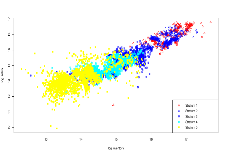
Figure 2: Scatter plot of log sales and log inventory data by strata

Figure 3: Regression model of $\log(y)$ against $\log(x)$ and strata indicator

To create missing, we considered univariate missing where only $y$ has missing values. We generated the response indicator $\delta$ of $y$ according to

$$\delta\sim Bernoulli(\pi),\ \pi=1/[1+\exp\{4-0.3\log(x)\}].$$

Under this model, the missing mechanism is MAR and the response rate is about $0.6$.

The parameters of interest are the stratum mean of $y$, $\eta_{h}=\mu_{h}$ for $1\leq h\leq 5$, and the population mean of $y$, $\eta_{6}=\mu$. The true parameter values are $\eta_{1}=92.25$, $\eta_{2}=67.90$, $\eta_{3}=18.24$, $\eta_{4}=13.01$, $\eta_{5}=5.92$, and $\eta_{6}=20.40$. The estimation methods included $(i)$ Full, the full sample estimator, which is used as a benchmark for comparison, $(ii)$ MI, the multiple imputation estimator with imputation size $M=100$, and $(iii)$ PFI, the parametric fractional imputation estimator with imputation size $M=100$, where the model parameters are estimated by the pseudo MLE solving the score equation (4).

To generate samples, we considered stratified sampling with simple random sampling within strata (STSRS) without replacement. Table 3 shows strata sizes $N_{h}$, sample sizes $n_{h}$, and sampling weights. The sampling weights range from $12.57$ to $45.79$. The samples are generated $2,000$ times.

Table 3: The sample allocation in stratified simple random sampling.

Strata	1	2	3	4	5
Strata size $N_{h}$	352	566	1963	2181	2198
Sample size $n_{h}$	28	32	46	46	48
Sampling weight	12.57	17.69	42.67	47.41	45.79

For MI, we considered the imputation models in (8.1). Because the sampling design is stratified random sampling and the imputation model includes the stratum indicator function, the sampling design becomes noninformative. We first imputed $\log(y)$ from the posterior distribution of (8.1), given the observed data, and then transformed the imputations to the original scale of $y$. The implementation of MI was carried out by the “mice” package in R. In each imputed data set, we applied the following full-sample point estimators and variance estimators: $\hat{\eta}_{1}=N^{-1}\sum_{h=1}^{H}N_{h}\bar{y}_{{h}}$ with $\bar{y}_{{h}}$ being the sample mean of $y$ in the $h$-th stratum $S_{h}$, $\hat{V}(\hat{\eta})=N^{-2}\sum_{h=1}^{H}N_{h}^{2}(1-n_{h}/N_{h})s_{{h}}^{2}/n_{h}$ with $s_{{h}}^{2}=(n_{h}-1)^{-1}\sum_{i\in S_{h}}(y_{hi}-\bar{y}_{{h}})^{2}$. For PFI, we considered the imputation model in (8.1). The proposal distribution in the importance sampling step is the imputation distribution evaluated at initial parameter values estimated from the available data. In PFI, for estimating model parameters, we obtained the pseudo MLEs by solving the score equations weighted by sampling weights, as in (4). After imputation, $\eta$ was estimated by (5) by choosing $U$ to be the corresponding estimating function. We used the delete-1 Jackknife replication method for variance estimation,

$$\hat{V}_{R}(\hat{\eta})=\sum_{h=1}^{H}\frac{n_{h}-1}{n_{h}}\sum_{i\in S_{h}}(\hat{\eta}^{[i]}-\hat{\eta})^{2},$$

where $\hat{\eta}^{[i]}$ is computed by omitting unit $i\in S_{h}$ and modifying the weights so that $w_{hj}$ is replaced by $n_{h}w_{hj}/(n_{h}-1)$ for all $j\in S_{h}$ and the weight remains the same for all other $j$.

Table 8 shows the numerical results. The mean and variance are calculated as the Monte Carlo mean and variance of the point estimates across the simulated sample data. The relative bias of the variance estimator is calculated as $\{(ve-var)/var\}$ $\times 100\%$, where $ve$ is the Monte Carlo mean of variance estimates and $var$ is Monte Carlo variance of point estimates. In addition, $95\%$ confidence intervals are calculated as $(\hat{\eta}-z_{0.975}\surd\hat{V},\hat{\eta}+z_{0.975}\surd\hat{V})$, where $z_{0.975}$ is the $97.5\%$ quantile of the standard normal distribution. The three estimators are essentially unbiased for point estimation. The variances for PFI and MI are close for all parameters. However, for inference, the validity of Rubin’s variance estimator relies on the congeniality condition (Meng 1994), which holds when MLEs are used as the full-sample estimator in MI, but not for Method-of-Moments estimators (MMEs) under MAR (Yang and Kim 2015b). As shown in Table 8, Rubin’s variance estimator of the MI estimator is biased upward for strata means and the population mean with relative bias $48.06\%$, $30.53\%$, $23.05\%$, $23.02\%$, $16.96\%$ for $\hat{\mu}_{j,MI}$, $1\leq j\leq 5$ and $32.75\%$ for $\hat{\mu}_{MI}$. Under the log normal distribution and MAR, the MMEs are not self-efficient and Rubin’s variance estimator is biased, which is consistent with the results in Meng (1994) and Yang and Kim (2015b). Among those, Stratum 1 has largest bias of the variance estimator, followed by Stratum 2, given their smaller sample sizes compared to other strata. In addition, the mean width of confidence intervals is larger than that of FI. For the population mean, we used the Horvitz–Thompson (HT) estimator as the full-sample estimator instead of the MLE under log-normal distribution. It is well-known that the HT estimator is robust but inefficient, which results in bias in Rubin’s variance estimator. The coverage of $95\%$ confidence interval reaches $98.3\%$ for the population mean due to variance overestimation. In contrast, PFI variance estimators applied to the HT estimator are essentially unbiased and provides empirical coverages close to the nominal coverage.

Numerical Results of Point Estimation (Mean and Var), Relative Bias (R.B.) of Variance Estimation, Mean Width and Coverage of $95\%$ Confidence Intervals (C.I.s) under Stratified Simple Random Sampling over $2,000$ Samples. The estimation methods include (i) FULL: the full sample estimator, (ii) MI: the multiple imputation estimator with imputation size $M=100$, (iii) PFI, the parametric fractional imputation estimator with imputation size $M=100$, where the model parameters are obtained by the pseudo MLE. The parameters are $\eta_{1}=$Stratum 1 mean, $\eta_{2}=$Stratum 2 mean, $\eta_{3}=$Stratum 3 mean, $\eta_{4}=$Stratum 4 mean, $\eta_{5}=$Stratum 5 mean, $\eta_{6}=$Population mean.

	Mean			Var			R.B. ($\%$)			Mean Width of C.I.s			Coverage
	FULL	MI	PFI	FULL	MI	PFI	FULL	MI	PFI	FULL	MI	PFI	FULL	MI	PFI
$\eta_{1}$	92.46	93.95	92.85	76.46	119.18	120.67	6.08	48.06	7.81	18.01	26.57	22.81	0.951	0.964	0.952
$\eta_{2}$	67.72	68.40	67.76	40.05	60.91	59.53	6.55	30.53	3.26	13.07	17.83	15.68	0.943	0.954	0.946
$\eta_{3}$	18.30	18.45	18.28	2.12	3.32	3.29	-3.06	23.05	-1.63	2.86	4.04	3.60	0.944	0.961	0.948
$\eta_{4}$	13.03	13.12	13.00	1.02	1.77	1.76	0.51	23.02	-4.28	2.03	2.95	2.60	0.946	0.962	0.943
$\eta_{5}$	5.92	5.98	5.91	0.22	0.46	0.46	1.84	16.96	-4.40	0.94	1.47	1.32	0.953	0.963	0.947
$\eta_{6}$	20.42	20.63	20.42	0.70	1.11	1.10	-3.36	32.75	-3.97	1.65	2.42	2.06	0.952	0.983	0.953

9 CONCLUDING REMARKS

In survey sampling, MI and FI are two available approaches of imputation for general-purpose estimation. In MI, Rubin’s variance estimation formula is recommended because of its simplicity, but it requires the congeniality condition of Meng (1994), which can be restrictive in practice. A merit of FI is that the congeniality condition is not needed for consistent variance estimation. When the sampling design is informative, MI can use an augmented model to make the sampling design noninformative. However, incorporating all design information into the model is not always possible (Reiter et al. 2006) and valid inference under MI is not easy or sometimes impossible (Berg et al. 2015). In contrast, FI can handle informative sampling design easily as it incorporates sampling weights into estimation instead of modeling.

So far, we have presented FI under the MAR case. Parametric FI can be adapted to a situation, where the missing values are suspected to be missing not at random (MNAR) (Kim and Kim 2012; Yang et al. 2013). A semiparametric FI using the exponential tilting model of Kim and Yu (2011b) is also promising, which is under development. Also, FI can be used to approximate observed log likelihood easily (Yang and Kim 2015a). The approximation of the observed log likelihood can be directly applied to model selections or model comparisons with missing data, such as using Akaike Information Criterion or the Bayesian Information Criterion. Further investigation on this topic will be worthwhile.

We conclude the paper with the hope that continuing efforts will be made into developing statistical methods and corresponding computational programs (an R software package is in progress) for FI, so as to make these methods accessible to a broader audience.

References

- Andridge and Little (2010) Andridge, R. R. and R. J. Little (2010). A review of hot deck imputation for survey non-response. Int. Stat. Rev. 78(1), 40–64.
- Bang and Robins (2005) Bang, H. and J. M. Robins (2005). Doubly robust estimation in missing data and causal inference models. Biometrics 61(4), 962–973.
- Berg et al. (2015) Berg, E., J. K. Kim, and C. Skinner (2015). Imputation under informative sampling. Submitted.
- Binder and Patak (1994) Binder, D. A. and Z. Patak (1994). Use of estimating functions for estimation from complex surveys. J. Amer. Statist. Assoc. 89(427), 1035–1043.
- Binder and Sun (1996) Binder, D. A. and W. Sun (1996). Frequency valid multiple imputation for surveys with a complex design. In Proceedings of the Survey Research Methods Section of the American Statistical Association, pp. 281–286.
- Breidt and Fuller (1996) Breidt, F. J., M. A. and W. A. Fuller (1996). Two-phase sampling by imputation. Journal of Indian Society of Agricultural Statistics (Golden Jubilee Number) 49, 79–90.
- Cao et al. (2009) Cao, W., A. A. Tsiatis, and M. Davidian (2009). Improving efficiency and robustness of the doubly robust estimator for a population mean with incomplete data. Biometrika 96(3), 723–734.
- Chen and Shao (2001) Chen, J. and J. Shao (2001). Jackknife variance estimation for nearest-neighbor imputation. J. Amer. Statist. Assoc. 96(453), 260–269.
- Durrant (2005) Durrant, G. B. (2005). Imputation methods for handling item-nonresponse in the social sciences: a methodological review. ESRC National Centre for Research Methods and Southampton Stat. Sci.s Research Institute. NCRM Methods Review Papers NCRM/002.
- Durrant (2009) Durrant, G. B. (2009). Imputation methods for handling item-nonresponse in practice: methodological issues and recent debates. International Journal of Social Research Methodology 12(4), 293–304.
- Durrant and Skinner (2006) Durrant, G. B. and C. Skinner (2006). Using missing data methods to correct for measurement error in a distribution function. Surv. Methodol. 32(1), 25.
- Fay (1992) Fay, R. E. (1992). When are inferences from multiple imputation valid? In Proceedings of the Survey Research Methods Section of the American Statistical Association, Volume 81, pp. 227–32.
- Fay (1996) Fay, R. E. (1996). Alternative paradigms for the analysis of imputed survey data. J. Amer. Statist. Assoc. 91(434), 490–498.
- Fuller (2003) Fuller, W. A. (2003). Estimation for multiple phase samples. In R. L. Chambers and C. J. Skinner (Eds.), Analysis of Survey Data, pp. 307–322. Chichester, U. K.: John Wiley & Sons.
- Fuller and Kim (2005) Fuller, W. A. and J. K. Kim (2005). Hot deck imputation for the response model. Surv. Methodol. 31(2), 139.