Validation of neural spike sorting algorithms without ground-truth information

Abstract

We describe a suite of validation metrics that assess the credibility of a given automatic spike sorting algorithm applied to a given electrophysiological recording, when ground-truth is unavailable. By rerunning the spike sorter two or more times, the metrics measure stability under various perturbations consistent with variations in the data itself, making no assumptions about the noise model, nor about the internal workings of the sorting algorithm. Such stability is a prerequisite for reproducibility of results. We illustrate the metrics on standard sorting algorithms for both in vivo and ex vivo recordings. We believe that such metrics could reduce the significant human labor currently spent on validation, and should form an essential part of large-scale automated spike sorting and systematic benchmarking of algorithms.

1 Introduction

One of the most powerful and widely used methods for studying neuronal activity in vivo (for example, in behaving animals) or ex vivo (for example, in extracted retinal preparations) is direct electrical recording. Using either single electrodes, tetrodes, or high-density multielectrode arrays, the experimental data consist of voltage patterns measured by sensors at the electrode tips, which are typically in the extracellular space. The strongest signals arise from an unknown but modest number of neurons in the immediate vicinity of each sensor, superimposed on a background consisting substantially of signals due to more and more distant, electrically shielded neurons [3]. Spike sorting is the name given to algorithms that detect distinct firing events and associate those events with specific neurons. The input consists of voltage traces from one or more electrodes and the output is a list of individual neurons that have been identified, as well as the spiking (firing) times for each. The literature on this subject is vast, and a very partial list of references includes [6, 8, 10, 11, 17, 28, 29].

In this environment, a typical data processing pipeline consists of (1) filtering the signal to remove high frequency noise and low frequency baseline drift, (2) spike detection, windowing and alignment, and (3) clustering based on the spike shape. The latter step, which is typically the core of the spike sorting algorithm, is predicated on the critical assumption that the electrical signals from distinct neurons have distinct “shapes,” discussed in more detail below. Finally, once the algorithm has assigned a neuron identity to each spike, various metrics are employed to assess the quality of the classification. In many experiments, the signals are, in fact, nonstationary. That is, the voltage pattern due to the firing of each neuron may vary over time. For the sake of simplicity, we will restrict our attention here to stationary data, but note that the framework for quality assessment that we introduce below does not depend on stationarity

Unfortunately, despite major progress in algorithms and software, spike sorting remains a labor-intensive task with a substantial manual component, both in the clustering and quality assessment phases. Furthermore, in the last two decades, the number of channels from which it is becoming possible to record simultaneously has grown from one (or a few) to thousands [6, 18, 27, 31]. As a result, it has become an urgent matter to accelerate the data analysis, to automate the clustering algorithms, and to develop statistical protocols that can provide robust estimates of the accuracy of the neuronal identification.

Despite some important work on validation, discussed in the next section, however, there are currently no established standards in the community either for estimating errors or for assessing the reproducibility of the output of spike sorting software. Moreover, as noted in [13, 23, 26, 32], it is of particular importance to be able to assess the fidelity of the output for each of the identified neurons separately. This is vital information in subsequent modeling, since the error rate from the spike sorting phase may permit the inclusion of some neurons and the exclusion of others when making inferences about neural circuitry, depending on the sensitivity of the question being asked.

In this paper, we concentrate on the problem of quality assessment, and propose a framework for estimating confidence in the results obtained from a black box spike sorting algorithm, in the absence of ground truth data such as an intra-cellular reference electrode. Since rigorous estimates of accuracy are not obtainable in this environment, we develop statistical measures of stability instead, drawing on ideas from bootstrapping and cross-validation in statistics and machine learning [30, 40, 41, 16, 36]. One of the important features of our framework is that quality estimation is carried out in an algorithm-agnostic fashion, not as an internal part of the spike sorting algorithm itself. This requires a standard interface for the data that is compatible with all (or most) algorithms, and the ability to invoke the spike sorting procedure without manual intervention. Our validation scheme, in fact, needs to be able to re-run the spike sorting software two or more times; see Fig. 1.

We hope that the stability metrics and neuron-by-neuron confidence measures described here will serve, in part, as a step toward systematizing the external evaluation of spike sorting algorithms and, in part, as motivation to fully automate the spike sorting process. Indeed, we see this as crucial to progress in the analysis of increasingly large scale electrophysiology data. Finally, we should note that we do not claim to present a novel algorithm for spike sorting—we will illustrate our metrics using conventional clustering and time series analysis tools.

The structure of this paper is as follows. In the remainder of the introduction we overview some existing approaches to validation (Sec. 1.1), then describe (Sec. 1.2) the two versions of spike sorting that we consider: the simpler sorting of individual spikes or “clips” (which have already been detected and aligned), and the more realistic sorting of a full time series. Standardizing the interfaces to these two algorithms is crucial for wide applicability of our metrics. Sec. 2 presents four schemes of increasing complexity for validating spike sorting on clips, and illustrates them on a standard PCA/k-means sorting algorithm applied to in vivo rodent data. Then Sec. 3 presents two schemes for validating the spike sorting of time series, and illustrates them on ex vivo monkey retina data. We discuss the implications and conclude in Sec. 4. Some methodological and mathematical details are gathered in the two appendices.

1.1 Prior work on quality metrics

As noted above, there has been substantial progress made over the last decade or so in developing methods for assessing the output of existing spike sorting methods. Broadly speaking, these consist of (a) statistical or information-theoretic measures of “isolation” of the clusters of firing events associated with each neuron and (b) physiological criteria for detecting errors such as refractory period violations. False positives are defined as firing events that are associated with neuron $j$, but should have been grouped with some other neuron $i$, with $i\neq j$. False negatives are defined as firing events that should have been associated with neuron $j$, but were either discarded or grouped with some other neuron. We do not seek to review these approaches here, and refer the reader to [13, 23, 26, 32]. While the establishment of such particular metrics is important, those of type (a) have until this point relied on accessing internal data (eg, PCA components) that are particular to certain types of algorithms while excluding many other successful approaches (eg, ICA, model-based fitting, and optimal filters).

Spike sorting algorithms can, of course, be run on simulated data, where ground truth is available. Thus, the development of more and more realistic forward models for neuronal geometry, neuronal firing, and instrumentation noise is an important goal [4]. Recently another approach has emerged, called “surrogate” spikes [21] or “hybrid datasets” [31], consisting of the original voltage recordings, to which are added new spikes (known waveforms extracted either from different electrodes in the same recording [21], or from a different recording with the same equipment [31]), at known times. Running the spike sorting procedure again on the new dataset provides a powerful validation test, particularly since it permits testing fidelity in the presence of overlapping spikes, which tend to result in errors using simple clustering schemes.

Despite all of these advances, however, most algorithms still involve manual intervention either at late stages of the clustering process or in quality assessment. While there have been some attempts to validate algorithms with human-operated steps [27], we believe that limiting human intervention to an early, exploratory phase, followed by a fully automated execution of the spike sorting software will be essential for establishing standards of reproducibility and quality, particularly with high-density multi-electrode arrays.

The related, and broader, problem of quality metrics in clustering algorithms has received much recent attention [16, 41, 36, 12]. However, many such metrics are not directly applicable to spike sorting, since they require access to internal variables that may be present in some algorithms and not others, and since they usually seek to assess the overall quality of the clustering (eg see [30]; for an exception, see [12]). In contrast, with spike sorting the concept of “overall quality” is not useful: there are often high-amplitude spikes that cluster well, plus a “tail” of spikes of decreasing amplitudes that cluster arbitrarily poorly, becoming indistinguishable from measurement noise. Thus, as realized by many researchers (eg [32, 25]), per-neuron metrics (as opposed to overall performance metrics) are crucial.

Figure 1: Interfaces and validation of automatic spike sorting algorithms. The algorithm $S$ to be validated is inside the “black box”, and is only accessible via the interface (a) or (b). In (a) the spike sorter assigns the $j$th clip a label (neural unit) $k_{j}$ from $1$ to $K$. In (b) the spike sorter acts on a whole time series $Y$ and returns a number $N_{s}$ of firing events (determined by the algorithm) described by labels $k_{j}$ and firing times $t_{j}$ in $[0,{T_{\mbox{\tiny tot}}}]$. (c) Overview of the validation scheme, applying to both clip-based and time series based algorithms, requiring the ability to rerun the algorithm $S$ as needed, and outputting the stability metric $f_{k}$.

1.2 Set-up of the problem and validation schemes

We consider interfaces to two spike sorting tasks (Fig. 1(a)–(b)). The first is a simple classification of isolated events, which will serve to introduce ideas, whereas the second is a rather general spike sorting interface:

1. The sorter classifies clips, ie short time-windows, each presumed to contain a single spiking event. We assume that the clips have already been extracted (by some detection process) and aligned (so that events of the same type occur at the same time within the clip). For each clip, an integer label is produced. More formally, let $X:=\{x_{mtj}\}_{m=1,\dots,M,\;t=1,\dots,T,\;j=1,\dots,N}$ be a three-dimensional array with $N$ clips, each of duration $T$ time samples and $M$ channels (electrodes). The sorting algorithm $S$ performs the map

   $$S(X)=\{k_{j}\}_{j=1}^{N}=:{\mathbf{k}}$$ (1)

   assigning a label (neuron identity) $k_{j}\in\{1,\dots,K\}$ to the $j$th clip. $K$ may be a fixed internal parameter of the algorithm, or may be a variable to be determined by the algorithm.

2. The sorter identifies all firing times and labels within a time-series $Y=\{y_{mt}\}_{m=1,\dots,M,\;t=0,\dots,{T_{\mbox{\tiny tot}}}-1}$, ie

   $$S(Y)=\{t_{j},k_{j}\}_{j=1}^{N_{s}}$$ (2)

   where $N_{s}$ is the number of spikes found (determined by the algorithm), while $t_{j}\in[0,{T_{\mbox{\tiny tot}}}]$ and $k_{j}\in\{1,\dots,K\}$ are their real-valued firing times and integer labels. In contrast to the clip-based interface, this allows $S$ to handle overlapping spiking events, which is crucial for complete event detection when firing rates are high [27, 25, 7].

The former interface captures the clustering task common to much software [17, 11, 31]. The latter encompasses essentially all types of automatic sorting algorithms, including those based on template matching [27, 21, 25, 7], ICA [34, 22] or filters [9], that have no simple detection step. Note that in neither interface are waveform shapes output, since these can be reconstructed from the inputs and outputs. We require that any algorithm parameters (thresholds, clustering settings, electrode information, etc) are fixed, and inaccessible via the validation interface.

Our key output comparison tool is the following matrix (see Fig. 1(c)). Given two size-$N$ lists of labels, $k_{j}\in\{1,\dots,K\}$, $j=1,\dots,N$, and $l_{j}\in\{1,\dots,L\}$, $j=1,\dots,N$, the confusion matrix (or contingency table [41, Ch.17]) is a rectangular matrix $Q$ whose $k,l$ entry is the number of spikes labeled $k$ in the first list and $l$ in the second, ie

$$Q_{k,l}\;:=\;\#\{j:k_{j}=k,l_{j}=l\}~{}.$$ (3)

Often the ordering of the labels is arbitrary, in which case we seek the “best” permutation of one of the sets of labels, in the sense of maximizing the sum of diagonal entries of the permuted $Q$ matrix. This best-permuted confusion matrix $\hat{Q}$ is defined by

$$\hat{Q}_{k,l}\;:=\;Q_{k,\hat{\pi}(l)}~{},\qquad\mbox{ where }\quad\hat{\pi}\;=\;\operatorname*{arg\,max}_{\pi\in S_{L}}\sum_{k=1}^{\min(K,L)}Q_{k,\pi(k)}$$ (4)

where $S_{L}$ is the set of permutations of $L$ elements. Large diagonal entries mean that the two sets of labels are consistent; off-diagonal entries indicate the amount and type of variation between the two labelings. The assignment problem of finding $\hat{\pi}$ can be solved in polynomial time by applying Kuhn’s “Hungarian algorithm” [15] to $-Q$. When firing times are also present, we will need an extended confusion matrix, which we postpone until section 3.

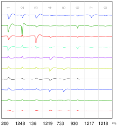
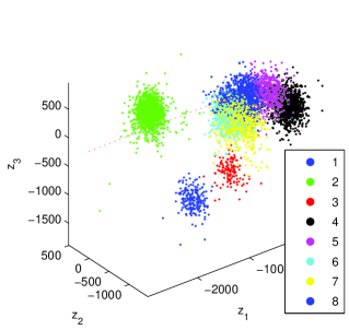
(a) (b) (c)

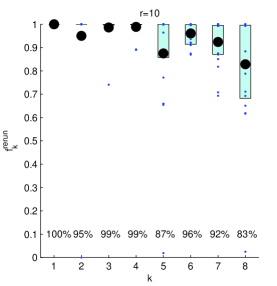
Figure 2: Spike-sorting of clips extracted from a rat motor cortex recording, using PCA/k-means++ (see section 2) with $K=8$ and best of $r=100$ repeats. (a) Average waveforms $W^{(k)}$ for $k=1,\dots,K$, (see (5)) with their populations (numbers of firings) $n_{k}$ shown below. Each of the $M=10$ channels is shown as a separate trace. The upwards-spiking channels are a result of spatial pre-whitening (App. A.1). (b) the labeling, each shown as a point in the feature space of the first three PCA components. Colors indicate label $k_{j}$ as in the inset. (c) 20 samples of the “rerun” stability metric of Sec. 2.2, for PCA/k-means++ with $K=8$ and $r=10$. The large dot (and percentage below) shows the mean $\bar{f}^{\mbox{\tiny rerun}}_{k}$, the small dots show all samples of $f^{\mbox{\tiny rerun}}_{k}$, and the bar shows their 25% to 75% quantiles.

2 Clip-based validation schemes

In this section we present some clip-based validation schemes, proceeding from simple to more sophisticated. Since there is no ground truth data, we must focus on the idea of stability. We make the point that if the labeling of a spike is unstable (with respect to resampling or perturbations consistent with the noise), then it is almost certainly not accurate. In other words, stability provides an upper bound on accuracy. We illustrate this on a set of 6901 upsampled and peak-aligned clips extracted from an in vivo rat motor cortex recording, as described in Appendix A.1.

2.1 A standard clip-based spike sorting algorithm

Since our goal is to validate existing algorithms rather than present new ones, we use as our default a standard spike-sorting algorithm that we refer to as PCA/k-means++, as follows. Clips are organized into a matrix $A\in\mathbb{R}^{MT\times N}$ such that each column contains the time-series for all channels for one clip. Dimension reduction (from dimension $MT=1470$ to dimension $N_{\mbox{\tiny fea}}=10$ by default) is then done by replacing each column by its first $N_{\mbox{\tiny fea}}$ PCA components. Then, treating each column (clip) as a point in $\mathbb{R}^{N_{\mbox{\tiny fea}}}$, k-means++ [1] is used for clustering, which requires a user-specified $K$. We remind the reader that k-means++ is a variant of k-means using a certain favorable random initialization of the centroids. The converged clustering produced often depends on initialization, ie the k-means iteration is not often able to find the global minimum of the sum of squared distances from points to their assigned centroids (this is in general $NP$-hard [1]). Thus, as is standard, we repeat k-means++ $r$ times and choose the repeat with the minimum sum of squared distances. The result is a label $k_{j}$ for each clip. The labels are permuted so that the $l_{2}$-norms of the estimated spike waveforms, ie $(\sum_{mt}[W^{(k)}_{mt}]^{2})^{1/2}$, decrease with increasing $k$. For this the estimated spike waveforms $W^{(k)}$ are found by simple averaging over all clips which have been assigned the same label $k$. More formally,

$$W^{(k)}_{mt}=\frac{1}{n_{k}}\sum_{j:k_{j}=k}x_{mtj}~{},\qquad m=1,\dots,M,\;t=1,\dots,T,\;k=1,\dots,K$$ (5)

where

$$n_{k}=n_{k}({\mathbf{k}}):=\#\{j:k_{j}=k\}$$ (6)

is the $k$th population in the labeling ${\mathbf{k}}$.

Fig. 2(a)–(b) shows the result of this sorting algorithm, for $K=8$ neurons and $r=100$ repeats, running on the clip dataset. Note that we do not claim that this is an optimal algorithm; our goal is merely to use it to illustrate the presented validation schemes.

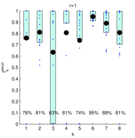
(a) (b) (c)

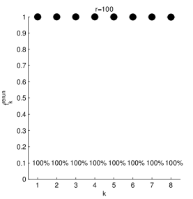
Figure 3: The “rerun” stability metric $f^{\mbox{\tiny rerun}}_{k}$ for PCA/k-means++ with $K=8$ fixed, for various $r$ (best of $r$ repeats of k-means++). (a) $r=1$, (b) $r=20$, (c) $r=100$. Plots should be interpreted as in Fig. 2(c). This shows convergence of all label stabilities to 1 (hence an uninformative metric) as $r$ increases.

2.2 A stability metric based on rerunning

Our goal is to validate a spike sorting algorithm acting on a particular dataset of clips. If the spike sorter is non-deterministic, then comparing two runs on exactly the same clip data (with different random seeds) gives a baseline measure of reproduceability for each label. Let $\{k_{j}\}={\mathbf{k}}$ and $\{l_{j}\}={\mathbf{l}}$ be the sets of labels returned from two such runs, and assume that they have the same number of labels $K$. Let $\hat{Q}_{k,l}$ be the elements of their best-permuted confusion matrix (4). Then define for each label $k$ the stability,

$$f_{k}:=\frac{2\hat{Q}_{k,k}}{n_{k}({\mathbf{k}})+n_{k}({\mathbf{l}})}~{},\qquad k=1,\dots,K.$$ (7)

Samples of $f_{k}$ are now computed by performing this process for many independent pairs of runs, with the same $K$, and the mean $\bar{f}_{k}$ is reported. We use the notation $f^{\mbox{\tiny rerun}}_{k}$ to indicate the “rerun” stability metric. Note that the pairs of runs used to sample the metric should not be confused with the $r$ “repeats” that are internal to this particular sorting algorithm $S$.

We illustrate this for our default sorting algorithm (using the best of $r=10$ k-means++ repeats) in Fig. 2(c), which shows 20 independent samples of $f^{\mbox{\tiny rerun}}_{k}$ with quantiles and means. This shows that the first four spike types are stable (as expected from the large waveform norms in panel (a) and well-separated clusters in (b)), while the last four are less so. The last ($k=8$) is the least stable, and from its tiny waveform it might be judged not to represent a single neural unit.

Remark 1.

We argue that 20 samples of any metric $f_{k}$ are more than sufficient for validation, because the resulting standard deviation of the estimator of the mean is then somewhat smaller than the width of the underlying distribution of $f_{k}$. If a neuron has a wide distribution of $f_{k}$, it is unstable, and high accuracy in estimating $\bar{f}_{k}$ is not needed. This follows wisdom from the Monte Carlo literature [20, Sec. 7.5].

However, as Fig. 3 shows, as a larger number of repeats $r$ is used, the stability for each label $k=1,\dots,K$ grows. By $r=100$ all stabilities have converged to very close to 1, ie there is very little variation in labeling due to random initialization. This is because picking the best of many repeats finds a sum of squares distances to centroids that is closer to the global minimum. The algorithm has effectively become deterministic, hence the rerun metric is uninformative. Since we wish to validate deterministic spike sorting methods (eg, ones based on hierarchical or density-based clustering [41, Ch. 14–15]), it is clear that one must introduce variation into the input $X$. We now turn to such methods.

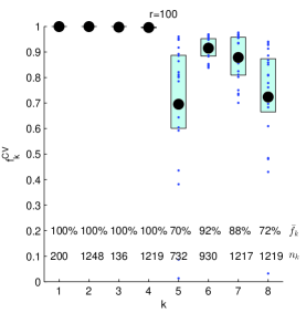
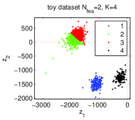
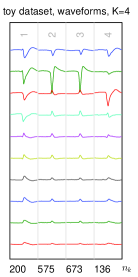
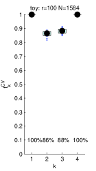
(a) (c) (b) (d) (e)

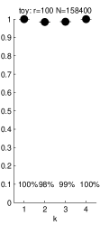
Figure 4: Three-way cross-validation stability metric for PCA/k-means++ (best of $r=100$ repeats). (a) Stabilities for $K=8$, and populations from a single run of the sorter. (b) The two PCA components of the “toy” data (extracted from the labels $k\leq 3$) with $N=1584$, labeled with PCA/k-means++ with $K=4$ and $N_{\mbox{\tiny fea}}=2$. (c) Estimated waveforms from the run shown in (b). (d) Stability metrics for the $K=4$ labels on the data from (b). (e) Same for an expanded dataset with a 100 times larger $N$.

2.3 A cross-validation metric using subsampling

In machine learning it is common to use cross-validation (CV) to assess an algorithm. The simplest version splits the data into training and test subsets, and uses the performance on the test set to estimate the generalizability of a classifier built using the training set. Although CV requires an observed dependent variable, a similar idea can be applied to spike sorting evaluation even in the absence of ground truth information. We divide the $N$ clips randomly into three similar-sized subsets I, II, and III, and train a classifier $C_{\mbox{\tiny I}}$ with only the data I, and a classifier $C_{\mbox{\tiny II}}$ with only the data II. Finally we compute the best-permuted confusion matrix (4) between the labels produced by classifying (labeling) the data III using $C_{\mbox{\tiny I}}$ and using $C_{\mbox{\tiny II}}$, then from this compute stabilities $f^{\mbox{\tiny CV}}_{k}$ for each spike type, as before using (7). Other more elaborate variants involving $m$-fold CV are clearly possible; we do not test them here.

We now describe the classifier. Our clip-based interface Fig. 1(a) does not include a classifier, yet we can build a simple one by taking the label of the mean waveform (5) that is closest (in some metric) to each clip in question. That is, given a set of clips $X$ which gives spike-sorted labels ${\mathbf{k}}=S(X)$, the estimated waveforms $W^{(k)}$, $k=1,\dots,K$ are computed via (5); they form the information needed for the classifier. Applying the classifier to new clips $X^{\prime}:=\{x^{\prime}_{mtj}\}$ gives new labels according to

$$k^{\prime}_{j}=\operatorname*{arg\,min}_{k\in\{1,\dots,K\}}\sum_{mt}(x^{\prime}_{mtj}-W^{(k)}_{mt})^{2}~{},$$

where for simplicity the $l_{2}$ norm has been chosen as the distance metric. Finally, since the waveform norm ordering of Sec. 2.1 may vary for independent subsamplings, then in order to collect meaningful per-label statistics of $f^{\mbox{\tiny CV}}_{k}$ we must permute the labelings from later repetitions to best match the first. For this we apply the Hungarian algorithm to the matrix of squared distances ($l_{2}$-norms) between all pairs of mean waveforms in the repetitions in question.

Fig. 4(a) shows this stability metric (for 20 independent 3-way splits) for the PCA/k-means++ spike sorter with $K=8$ and $r=100$. Notice that the last four spike types have stabilities in the range 70–90%, in contrast to Fig. 3(c) for which they were all 100%. This shows that the three-way data subsampling introduces variation that detects unstable label assignments, even for an essentially deterministic spike sorter.

We now show that the 3-way CV metric is able to identify an erroneously split cluster. For this we generate a simple “toy” dataset comprising just the $N=1584$ clips with labels $k_{j}=1$, 2 or 3 from the default $K=8$ and $r=100$ spike sorting (Fig. 2). Thus there are three very well-separated true clusters in feature space with a clear ground-truth; see Fig. 4(b). For this toy dataset we pick a standard sorting algorithm of PCA/k-means++ with $K=4$ (chosen to be erroneously large), $r=100$, and $N_{\mbox{\tiny fea}}=2$ (to aid visualization). Running this algorithm on the toy data gives the labeling in two dimensions of feature space shown in Fig. 4(b), and waveforms of Fig. 4(c): the largest true cluster is erroneously split into two nearly-equal pieces, which are given new labels $k=2,3$ (hence the similar pair of waveforms in (c)). There are many ways to summarize accuracy here [41, Sec. 17.3.1]: filling the confusion matrix (4) of size $3\times 4$ between truth and the $K=4$ clustering gives the F-measures (7) for the three true labels as $f_{2}=0.701$, $f_{1}=f_{3}=1$. Running the CV metric on this $K=4$ sorting algorithm results in the stabilities in Fig. 4(d): a mean around 87% for $k=2,3$ (somewhat higher than measures of accuracy), and 100% for the other (unsplit) clusters. The point of our framework is that this conclusion is reached via only the standard interface $S$, ie without access to the feature vectors shown in (b), nor of course the ground truth.

However, the variation in labeling induced by subsampling is small compared to the known accuracy (one reason being that the small $N_{\mbox{\tiny fea}}$ makes for high stability), and furthermore dies away as the number of clips grows, $N\to\infty$. We illustrate this in Fig. 4(e), which shows the 3-way CV metric for the same algorithm as (d) but running on a set of clips 100 times larger, generated as described in App. A.2. The stabilities of the $k=2,3$ labels of the split cluster are now around 98.5%, hardly an indication of instability. This is consistent with a central limit theorem proven [33] for stability metrics in a wide class of clustering algorithms, when their global optimum is unique, implying in our setting that

$$1-f^{\mbox{\tiny CV}}_{k}={\mathcal{O}}(N^{-1/2}),\qquad\mbox{ for each $k$}~{}.$$

Indeed, increasing $N$ by a factor of 100 decreased the deviation of $f_{k}$ from unity by around a factor of 10. We expect the prefactor for this deviation to be smaller when the split cluster is more non-spherical: resampling induces high instability in splitting a spherical cluster, but in k-means a non-spherical cluster (as in Fig. 4(b)) tends to split consistently along a hyperplane perpendicular to its longest axis.

This unfortunate phenomenon that, regardless of the apparent quality of the labeling, stability tends to unity as $N$ grows has been known in the clustering literature for some time [14]. Renormalizing a global stability metric by $\sqrt{N}$ is possible [36, Sec. 3.1.1], but it is not clear how to do this when a per-neuron metric is needed. On the other hand, restricting to small-$N$ subsamples to induce instability has the major disadvantage that the spike sorter is then never validated with any dataset of the desired size.

Since we seek a scheme which can validate spike sorting applied to arbitrarily large datasets, we must move beyond subsampling, and explore perturbing the clips themselves.

       
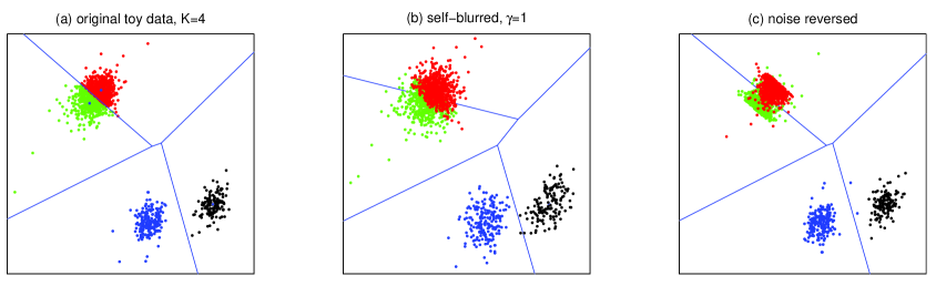
  (e)                                            (f)

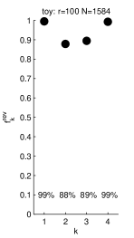
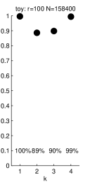
Figure 5: Data perturbation validation metrics illustrated on the “toy” clips (from labels $k\leq 3$), sorted with PCA/k-means++ with $K=4$, $r=100$, $N_{\mbox{\tiny fea}}=2$. (a)–(c) shows the 2D PCA feature space. (a) Original points labeled by color as in Fig. 4(b), showing k-means centroids and decision boundaries. (b) Points after self-blurring and (c) after noise reversal; colors show the original labelings, to highlight movement, and new decision boundaries. (d) Idealized 1D picture: only the shaded parts of the distribution change labeling. Stability metrics are shown for (e) self-blurring and (f) noise reversal, for the original toy data size $N$, and a 100 times larger $N$.

2.4 Metrics based on data perturbations without subsampling

Fig. 4(b)–(e) shows that for large $N$, stability under subsampling fails to indicate a highly erroneous split cluster. By examining feature space (Fig. 4(b)) it is clear that a decision boundary of k-means passes through a high-density region. Can one create a metric that quantifies this undesirable property without access to feature space, using only the standard interface? We now present two such metrics, both of which involve perturbing the data.

2.4.1 Self-blurring

Firstly we describe a method that we name self-blurring for reasons that will become clear. Let ${\mathbf{k}}=S(X)$ be the output of the sorter on the full set of clips, and $\{W^{(k)}\}_{k=1,\dots,K}$ be the mean waveforms found via (5). Let $\pi$ be a permutation of the $N$ clips that randomizes only within each label class. Precisely, if $J_{k}:=\{j:k_{j}=k\}$ is the index set of the $k$th label type, and $\pi_{k}$ is a random permutation of $n_{k}$ elements, then the overall permutation $\pi$ is defined by

$$\pi(J_{k}(i))\;=\;J_{k}(\pi_{k}(i)),\qquad i=1,\dots,n_{k}$$

holding for each label type $k=1,\dots,K$. From this we create a perturbed clip dataset $\tilde{X}$ with elements

$$\tilde{x}_{mtj}\;=\;x_{mtj}+\gamma(x_{mt,\pi(j)}-W^{(k_{j})}_{mt}),\qquad m=1,\dots,M,\;t=1,\dots,T,\;j=1,\dots,N,$$ (8)

where $\gamma>0$ is a parameter controlling the size of the perturbation. Running the sorter on this new data gives $\tilde{{\mathbf{k}}}=S(\tilde{X})$, then we compute the best-permuted confusion matrix (4) between labels ${\mathbf{k}}$ and $\tilde{\mathbf{k}}$, and from it obtain the per-label stabilities $f_{k}^{\mbox{\tiny blur}}$ via (7).

The bracketed expression in (8) can be interpreted as a random sample from the “noise distribution” of the $k_{j}$th cluster in clip signal space, relative to its mean waveform (centroid). So, with $\gamma=1$, the cluster distribution about its centroid is convolved (blurred) with itself. The result is that, even if a decision boundary remains fixed, if there is density near this boundary then points are carried across it by the convolution, thus change label, and are registered as instability. The new data $\tilde{X}$ is consistent with the original $X$ in the sense that it differs only by additive noise of exactly the type observed within each cluster. No assumption on the form of the noise model or noise level is made.

Since $\mathbb{R}^{MT}$ (signal space) is hard to visualize, we again “peek under the hood” of our PCA/k-means++ algorithm, by in Fig. 5(b) showing the result of self-blurring on the 2D feature vector points. Notice that there is significant overlap of red and green points, and rotation of one of the decision lines. The self-convolution also results in larger clusters, which may cause label exchange between clusters that were distinct (eg see the tails of the lower two clusters). For an isolated Gaussian cluster, its size (noise level) grows by a factor $\sqrt{2}$. Fig. 5(e) shows the distribution of $f_{k}^{\mbox{\tiny blur}}$ for 20 samples of $\tilde{X}$. The mean around 75% for $k=2,3$, being similar to the actual F-measure accuracy of 70%, is a clear indicator of instability. For the dataset of size $100N$ this also holds; thus, we have cured the large-$N$ vanishing of instability present with CV.

We show an idealized example where points are drawn from a symmetric distribution $p(z)$ in a 1D variable $z$, erroneously split into two clusters, in the top two pictures in Fig. 5(d). The decision boundary is unchanged by self-blurring. The mass of each half of the distribution that changes label is shaded; this controls the size of $1-f_{1}^{\mbox{\tiny blur}}$. If this distribution were a Gaussian, and $\gamma=1$, we can solve analytically (see App. B) that $f_{1}^{\mbox{\tiny blur}}=1-[\operatorname{erf}((2\pi)^{-1/2})]^{2}\approx 0.817$. The same holds for a multivariate Gaussian in signal space split along a plane of symmetry. The reported stabilities in Fig. 5(e) also are similar to this value, even though clusters are not expected to be Gaussian [8].

Later we will vary $\gamma$: a smaller $\gamma$ tends to increase all reported stabilities, but also causes less inflation of clusters (ie less increase in noise level), which may better reflect an algorithm’s stability for close, but distinct, clusters.

2.4.2 Noise reversal

Our second perturbation method has a similar flavor: using the above idea of noise (deviation) relative to a cluster centroid, we simply negate the noise. That is, we replace (8) by

$$\tilde{x}_{mtj}\;=\;2W^{(k_{j})}_{mt}-x_{mtj}~{},\qquad m=1,\dots,M,\;t=1,\dots,T,\;j=1,\dots,N,$$ (9)

and proceed exactly as above to get $f_{k}^{\mbox{\tiny rev}}$. Since this is a deterministic procedure, there is no need to resample; only two spike sorter runs are needed (the original and the noise-reversed). This is shown in Fig. 5(c), and lower picture of (d): each cluster is inverted about its centroid. Label exchange occurs in a split cluster because the tails of the distributions are made to point inwards, and bleed across the boundary. The results for this toy dataset appear in Fig. 5(e): the erroneously-split labeling induces around 89% stability for both the original $N$ and a 100 times larger $N$. This is more stable than both self-blurring and the true accuracy—a disadvantage—however its advantages are that the clusters are not artificially enlarged, that there are no free parameters, and no resampling.

In the idealized 1D Gaussian case, and the multivariate Gaussian split along a symmetry plane, analytically (see App. B) we get $f_{1}^{\mbox{\tiny rev}}=\operatorname{erf}(2/\sqrt{\pi})\approx 0.889$, which is very close to the observed values, and explains why stabilities are expected to be closer to 1 than for self-blurring with $\gamma=1$.

(a)

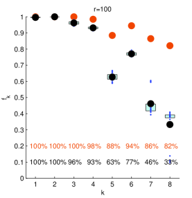
(b)

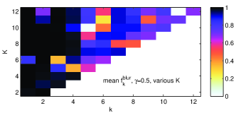
(c)

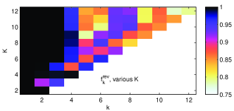
(d)

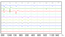
(e)

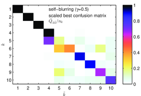
Figure 6: Perturbation metrics for default clips dataset with PCA/k-means++ with $r=100$. (a) self-blurring ($\gamma=1$, shown in black) and noise reversal (shown in orange) metrics for $K=8$. (b) self-blurring ($\gamma=0.5$) metric $\bar{f}_{k}^{\mbox{\tiny blur}}$ for various $K=2,\dots,12$ (each row a different $K$). (c) same for noise reversal metric $f_{k}^{\mbox{\tiny rev}}$. (d) mean waveforms for $K=10$, and (e) self-blurring scaled best confusion matrix $\hat{Q}_{k,\tilde{k}}/n_{k}$.

2.4.3 Perturbation metric tests for the default algorithm

We return to the full clips data from Sec. 2.1 with PCA/k-means++ with the default $N_{\mbox{\tiny fea}}=10$ and $r=100$. Fig. 6(a) compares the self-blurring and noise reversal metrics for $K=8$: we see that noise reversal has all stabilities roughly 3 times closer to unity than self-blurring at $\gamma=1$, but otherwise similar relative stabilities vs neuron label $k$.

Since we cannot presume that $K=8$ is optimal for extracting the largest number of stable neurons, in Fig. 6(b)–(c) we show the mean stabilities varying $K=2,\dots,12$. Both show that the first four neurons are stable for most $K$ values, and show that one or two others are also quite stable for $K\geq 8$ (these are neurons $k=7,8$ for $K\geq 10$). Notice that, for noise reversal, no stabilities drop below 0.75, ie the stability range is compressed towards unity.

We study $K=10$ in more detail, since for it, neuron $k=5$ shows a self-blurring stability close to zero. Fig. 6(d) shows the mean waveforms for this $K$; indeed $k=4,5$ have very similar waveforms so would probably be deemed erroneously split in practice. The (best-permuted) confusion matrix $\hat{Q}$ is a useful diagnostic: as the vertical “domino” in Fig. 6(e) shows, $k=4$ and 5 have been merged by self-blurring. Off-diagonal entries such as $\hat{Q}_{6,9}$ show that $k=6,9$ are prone to mixing, which is borne out by their visually similar waveforms. The point is that our metrics quantify such judgments, without a human having to examine whether waveforms are “close” given the particular noise (and firing variation) of the experiment.

Finally, we observe that for $K=4$, all supposed neurons are very stable (under both metrics), even though, with our knowledge of the larger number of distinct waveforms extracted for greater $K$, it is obviously not accurate. This illustrates that stability is necessary but not sufficient for accuracy.

Remark 2.

Although we illustrated the self-blurring and noise reversal metrics with a label assignment (clustering) scheme involving hard decision boundaries (hyperplanes for k-means), we propose a broader view: since both metrics involve perturbing the clip data in a manner consistent with the noise, any reproducible neural unit output by a spike sorting algorithm should be stable under these metrics.

3 Time-series based validation schemes

We now turn to the second, more general, interface of Sec. 1.2, where the spike sorter extracts both times $t_{j}$ and labels $k_{j}$ from a time series $Y$ of multi-channel recorded data. To compare two outputs of such a sorter, say $\{t_{j},k_{j}\}_{j=1}^{N_{s}}$ and $\{t^{\prime}_{j},k^{\prime}_{j}\}_{j=1}^{N_{s}^{\prime}}$, where $k_{j}\in\{1,\dots,K\}$, $k^{\prime}_{j}\in\{1,\dots,K^{\prime}\}$, and $K$ and $K^{\prime}$ are the two (not necessarily equal) numbers of types of neurons found, one must match spikes from the first run to those in the second. A simple criterion is that matched firing times be within $\epsilon$ of each other; we fix $\epsilon=0.5$ ms in our tests. Specifically, let a matching $\mu$ be a one-to-one map from a subset of $\{1,\dots,N_{s}\}$ to an (equal-sized) subset of $\{1,\dots,N^{\prime}_{s}\}$ such that

$$|t_{j}-t^{\prime}_{\mu(j)}|\leq\epsilon~{},\qquad\mbox{for all $j$ matched in the map.}$$ (10)

Given any such $\mu$, the confusion matrix is defined by

$$Q^{(\mu)}_{k,k^{\prime}}=\#\{j:\mu(j)\mbox{ exists},\;k_{j}=k,\;k^{\prime}_{\mu(j)}=k^{\prime}\}~{},\qquad\mbox{ for }1\leq k\leq K,\;1\leq k^{\prime}\leq K^{\prime}~{}.$$ (11)

Since there may be unmatched spikes $j$ in the first run (for which we write $\mu(j)=\varnothing$), and unmatched spikes $j^{\prime}$ in the second run (for which we write $\mu^{-1}(j^{\prime})=\varnothing$), a row and column is appended for these cases to $Q^{(\mu)}$, ie,

$$Q^{(\mu)}_{k,\varnothing} = \#\{j:\mu(j)=\varnothing,\;k_{j}=k\}~{},\qquad\mbox{ for }1\leq k\leq K~{},$$ (12)

$$Q^{(\mu)}_{\varnothing,k^{\prime}} = \#\{j:\mu^{-1}(j^{\prime})=\varnothing,\;k^{\prime}_{j^{\prime}}=k^{\prime}\}~{},\qquad\mbox{ for }1\leq k^{\prime}\leq K^{\prime}~{},$$ (13)

and set $Q^{(\mu)}_{\varnothing,\varnothing}=0$. The $(K+1)$-by-$(K^{\prime}+1)$ matrix $Q^{(\mu)}$ defined by (11)–(13) we call the extended confusion matrix; see Fig. 7(a).

Since a sorting algorithm may arbitrarily permute the neuron labels, as before we need to find the “best” confusion matrix. However, now one must search over permutations $\pi$ of the second label and over matchings $\mu$, ie find

$$\hat{Q}_{k,k^{\prime}}:=Q^{(\hat{\mu})}_{k,\hat{\pi}(k^{\prime})}~{},\qquad\mbox{ where }\quad\{\hat{\mu},\hat{\pi}\}=\operatorname*{arg\,max}_{\mu\in{\cal M},\pi\in S_{K^{\prime}}}\sum_{k=1}^{\min(K,K^{\prime})}Q^{(\mu)}_{k,\pi(k)}~{},$$ (14)

where ${\cal M}$ is the set of all maps $\mu$ satisfying (10). In practice we find that a simple three-pass algorithm performs well at typical firing rates (optimizing $\pi$ using a greedy-in-time-difference algorithm for matching, then with $\pi$ fixed, optimizing $\mu$ via two passes of greedy matching). We do not know the complexity of finding the exact solution.

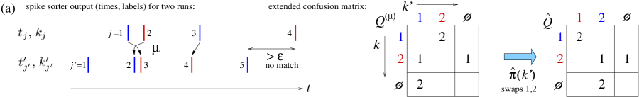
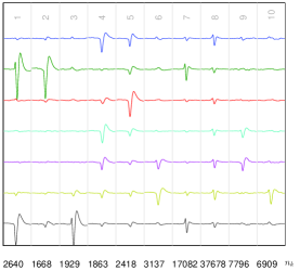
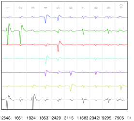
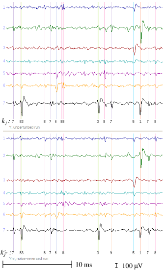
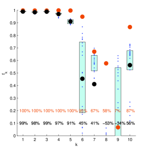
(b) (c) (d)   (e) (f)

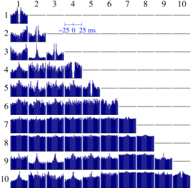
Figure 7: Time-series stability metric results. (a) Toy example ($K=2$) of a matching $\mu$ between one spike sorter output $t_{j}$, $k_{j}$ and another $t^{\prime}_{j^{\prime}}$, $k^{\prime}_{j^{\prime}}$ (blue shows label $k=1$ and red label $k=2$). The resulting extended confusion matrix and its “best” permutation $\hat{Q}$ are shown. The matching $\mu$ shown is the best matching $\hat{\mu}$ even though the nearby pair is swapped in time. (b)-(f) show results for the spike sorter of Sec. 3.1 with $K=10$. (b) Waveform shapes $\{V^{(k)}\}_{k=1}^{K}$ and populations from the unperturbed run, and (c) from the noise-reversed run. (d) Input time series data $Y$, and noise-reversed time series $\tilde{Y}$, showing firing times and (best-permuted) labels from each run. (e) Stability metrics $f_{k}$ for noise-reversal (shown in orange), and for the spike addition metric (black). (f) Spike firing cross-correlations of spike sorter output $t_{j}$, $k_{j}$. Refractory dips (of at least $\pm 3$ ms) are complete for $k=1,\dots,5$ and partial for $k=6,10$, matching the metrics in (e).

3.1 A simple time-series spike sorting algorithm

As an illustrative spike sorter we will use the following model-based fitting algorithm which handles overlapping spikes (the full description we leave for a future publication). We assume that the time series $Y$ has been low-pass filtered. Firstly, upsampled clips are extracted from $Y$ using the triggering and upsampling procedure of App. A.1, with a $-100$ $\mu$V threshold. Secondly, these clips are fed into the clip-based spike sorter of Sec. 2.1, using the best of $r=100$ repetitions of k-means++, with a preset number of clusters $K$. Thirdly, a set of upsampled mean waveform shapes $\{W^{(k)}\}_{k=1}^{K}$ is found by applying (5) to the resulting clips and labels. These waveforms are ordered by descending $l_{2}$-norm. Finally, these waveforms are matched to the complete time series $Y$ via a greedy fitting algorithm [27, 25]. Specifically, the change in $l_{2}$-norm of the residual due to subtraction of each (downsampled, fixed-amplitude) waveform at each time-shift was computed, and firing events $t_{j}$ were declared at sufficiently negative local minima (wth respect to time shift) of this function, that were also global minima over all waveforms with time shifts up to $\pm 0.5$ ms from $t_{j}$. The corresponding $k_{j}$ was the label of the waveform responsible for this largest decrease in residual. This greedy sweep through the time series was repeated until no further change occurred. Note that, as with many modern algorithms [34, 9, 7, 22, 25] the main fitting stage involves no concept of “clips” or event windows.

As in Sec. 2.2, a simple rerunning validation metric would be possible for time series. However, we present the following two metrics as much more realistic indicators of stability.

3.2 Noise-reversal

The noise-reversal idea of Sec. 2.4.2 generalizes to time series, handling overlapping spikes naturally, as follows. Firstly, the sorter runs on the unperturbed data to give $S(Y)=\{t_{j},k_{j}\}_{j=1}^{N_{s}}$. Since the interface does not output waveforms, they are next estimated by averaging windows from $Y$ centered on the output firing times $t_{j}$ for the appropriate label, eg

$$V^{(k)}_{mt}\;=\;\frac{1}{n_{k}}\sum_{j:k_{j}=k}y_{m,t_{j}+t-T/2}~{},\qquad m=1,\dots,M,\;t=1,\dots,T~{}.$$ (15)

The “forward model” generating a (noise-free) time series from a new set of firing times ${\mathbf{s}}:=\{s_{j}\}_{j=1}^{N}$ and labels ${\mathbf{l}}:=\{l_{j}\}_{j=1}^{N}$ is then $F({\mathbf{s}},{\mathbf{l}})$, with entries

$$F_{mt}=F({\mathbf{s}},{\mathbf{l}})_{mt}\;:=\;\sum_{j=1}^{N}V^{(l_{j})}_{m,t-s_{j}+T/2}~{},\qquad m=1,\dots,M,\;t=1,\dots,{T_{\mbox{\tiny tot}}}~{}.$$ (16)

(We in fact use variants of (15)–(16) which achieve sub-sample firing time accuracy by upsampling the waveforms $V^{(k)}$ as in App. A.1, and building downsampling into $F$.) Using this, a perturbed time series (analogous to (9)) is generated,

$$\tilde{Y}\;=\;2F({\mathbf{t}},{\mathbf{k}})-Y~{},$$ (17)

and sorted to give $S(\tilde{Y})=\{t^{\prime}_{j^{\prime}},k^{\prime}_{j^{\prime}}\}_{j^{\prime}=1}^{N_{s}^{\prime}}$. Finally, the best extended confusion matrix $\hat{Q}$ between the two sets of outputs is found as in (11)–(14), and the usual stability metric $f_{k}$ computed via (7).

Fig. 7 illustrates this metric for spike sorting filtered time series data $Y$ taken from an ex vivo retinal multi-electrode array recording described in App. A.3, with $K=10$ neurons assumed. This dataset has a large fraction of overlapping events: spike sorting as in Sec. 3.1 results in around 10% of firing events falling within 0.1 ms of another event. The upper half of Fig. 7(d) shows a short time window from $Y$, while the lower half shows the resulting $\tilde{Y}$. Note that some of the sorted times and labels have changed, while between firing events the signal is negated. The orange dots in Fig. 7(e) show the resulting $f_{k}^{\mbox{\tiny rev}}$ values: the five neurons with largest waveform norms are quite stable, while $k=6$ and $10$ are marginally stable (recalling from Sec. 2.4.2 that $90\%$ is hardly a stable noise-reversal metric), and $k=7,8,9$ are unstable and—judging by their huge $n_{k}$—massively overfit. This matches well the per-neuron physiological validation based on clarity of refractory dips in the firing time auto-correlations in Fig. 7(f).

It is worth examining why $k=9$ has almost zero stability. The cause is apparent in panels (b)-(c), which show the waveforms $V^{(k)}$ estimated via (15) from the unperturbed and noise-reversed runs (the latter in “best permuted” ordering $\hat{\pi}$). The two sets of waveforms are very similar apart from the possibly distinct neuron $k=9$ in (b) which has disappeared in (c) due to the splitting of $k=7$. We find that such clustering instabilities are common, and vary even with rerunning the sorter with a different random seed in k-means++. Our metric quantifies these instabilities as induced by variations consistent with any even-symmetric noise model.

3.3 Auxiliary spike addition

The final stability metric we present perturbs the time series by linearly adding new spikes at known random firing times and then measuring their accuracy upon sorting; this gauges performance in the context of overlapping spikes—by creating and assessing new overlaps—while respecting the linearity of the physical model for extracellular signals [3].

Let the first uperturbed sorter run produce times and labels $S(Y)=\{t_{j},k_{j}\}_{j=1}^{N_{s}}$, from which a forward model is built, as above via (15)–(16). An estimate for the firing rate of the $k$th neuron is $n_{k}/{T_{\mbox{\tiny tot}}}$, where $n_{k}$ is given by (6). One generates an auxiliary set of events $\{s_{j},l_{j}\}_{j=1}^{N_{a}}$ as the union of $K$ independent random Poissonian spike trains, with rates $\beta n_{k}/{T_{\mbox{\tiny tot}}}$, $k=1,\dots,K$, where $\beta$ is a rate scaling parameter. If $\beta$ is too small, not much is learned from the perturbation; if too large, the total firing rates are made unrealistically large. We fix $\beta=0.25$. The perturbed time series is then

$$\tilde{Y}\;=\;Y+F({\mathbf{s}},{\mathbf{l}})~{},$$ (18)

which is sorted to give $S(\tilde{Y})=\{t^{\prime}_{j^{\prime}},k^{\prime}_{j^{\prime}}\}_{j^{\prime}=1}^{N_{s}^{\prime}}$. The best extended confusion matrix $\hat{Q}$ is now found (as in (11)–(14)) between the total of $N_{s}+N_{a}$ events ${\mathbf{t}}\cup{\mathbf{s}},\,{\mathbf{k}}\cup{\mathbf{l}}$, and the second run outputs ${\mathbf{t}}^{\prime},{\mathbf{k}}^{\prime}$. To assess the change in $\hat{Q}$ induced by adding spikes, we compute the matrix

$$\hat{Q}^{\mbox{\tiny add}}\;:=\;\hat{Q}-\operatorname{diag}\{n_{1},\dots,n_{K},0\}$$

where $\operatorname{diag}$ denotes the diagonal matrix with diagonal elements as listed. Finally, $f_{k}^{\mbox{\tiny add}}$ is computed as in (7) using $\hat{Q}^{\mbox{\tiny add}}$. One may interpret this diagonal subtraction as follows: if all the new spikes were correctly sorted, and all the original spikes sorted as in the first run, $\hat{Q}^{\mbox{\tiny add}}$ would be diagonal with entries given by the added populations for each label, so $f_{k}^{\mbox{\tiny add}}=1$ for all $k$. Thus low $f_{k}^{\mbox{\tiny add}}$ values indicate either lack of sorting accuracy for the added spikes, or induced instability (eg false positives or negatives) in re-sorting the original spikes. Both of these are important warning signs that a putative neuron is less believable.

Remark 3.

Marre et al. [21] and Rossant et al. [31] use similar but distinct validation metrics: they add spikes with known firing times from either a spatially translated neuron, or a “donor” neuron from a different recording, then assess accuracy for this neuron. While useful as overall measures of reliability, these methods require dataset-specific adaptations, and it is not clear that they validate any of the particular neurons in the original data. In contrast, the metric we propose here validates each neuron as sorted in the dataset of interest.

Fig. 7(e) shows 20 independent samples of $f_{k}^{\mbox{\tiny add}}$ (ie, 20 realizations of the Poisson spike trains), with the black dots showing the means. Only the first five neurons have stabilities above 60%. The overall pattern is similar to noise-reversal, but with a lower overall calibration of the metric, and it matches well the independent validation via cross-correlations in Fig. 7(f). Note that if adding a certain type of spike induces changes in the sorting of the (more numerous) existing spikes, then huge drops in stability, including highly negative $f_{k}^{\mbox{\tiny add}}$, are possible, as visible in Fig. 7(e), $k=8,9$. Indeed, from its waveform and huge population in Fig. 7(b), $k=8$ would likely be classified as the “noise cluster” (see eg [38]) by an experienced human.

Interface	Metric	Section	Advantages	Disadvantages
clip based	rerun	Sec. 2.2	simplicity	useless if sorter is deterministic
	3-way CV	Sec. 2.3	simplicity	classifier needed; not useful for large $N$
	self-blurring	Sec. 2.4.1	adjustable parameter $\gamma$	raises noise level (can underestimate accuracy)
	noise reversal	Sec. 2.4.2	only needs 2 runs; no extra noise	stability range close to 1
time series	noise reversal	Sec. 3.2	only needs 2 runs; no extra noise	stability range close to 1; reverses noise polarity
	spike addition	Sec. 3.3	accuracy in context; no extra noise	firing rate slightly higher; no built-in shape variation

Table 1: Summary of the proposed validation metrics for clip-based and time series spike sorting algorithms.

4 Discussion and conclusions

We have proposed several schemes for the validation of automatic spike sorting algorithms, each of which outputs a per-neuron stability metric in the context of the dataset of interest, without ground truth information or physiological criteria, and with few assumptions about the noise model. Our key contribution is a common framework (Fig. 1) where this validation occurs only through a simple standardized interface to the sorter, which is treated as a black box that can be invoked multiple times. We see this as essential to automated validation and benchmarking of a growing variety of spike sorting algorithms and codes. By contrast, most existing validation metrics rely, in part, on accessing internal parameters peculiar only to certain algorithms. We also envisage such metrics as the first filter in a laboratory pipeline in which—due to the increasing scale of multi-electrode recordings—it will be impossible for a human operator to make decisions about most neurons. While stability cannot guarantee accuracy or single-unit activity (eg see Sec. 2.4.3), instability is a useful warning of likely inaccuracy or multi-unit activity. Only neurons that pass the stability test should then be further validated based on eg shape [35], refractory gaps [13] and/or receptive fields [19, 21, 25].

Table 1 summarizes the six schemes: the first four use a simple sorting interface that classifies “clips” (spiking events), while the remaining two use a more general interface that accesses the full time series and allows handling of overlapping spikes. All schemes resample or perturb the data in a realistic way, then measure how close the resulting neuron-to-neuron best confusion matrix $\hat{Q}$ is to being diagonal; its off-diagonal structure also indicates which neurons are coupled by instabilities. Although our demonstrations used standard sorting algorithms with a specified number of neurons $K$, the metrics also apply to variable $K$ with minor extra bookkeeping.

The first two schemes (rerunning and cross-validation) are conceptually simple but are shown to have severe limitations. The next two (self-blurring and noise reversal for clip sorting) seem useful even in large-scale settings. However, we expect that the last two (noise reversal and spike addition for time series) will be the most useful. Each metric carries its own calibration: for instance, with the sorter fixed, for noise reversal $f_{k}$ is much closer to 1 than for spike addition. A future task is to calibrate the metrics against accuracy with both synthetic and ground-truth data.

Although general, our schemes make certain assumptions. Noise reversal assumes sign-symmetry in the noise distribution (which may not be satisfied for “noise” due to distant spikes), whereas spike addition as presented does not account for realistic firing variation in the added spikes; the latter could be achieved in a model-free way by adding random spike instances (as in self-blurring) instead of mean waveforms.

We believe that several other extensions are worth exploring. 1) The last two validation schemes essentially involve reverse-engineering a forward model (16) from a single spike sorter run. This model could be improved in various ways, by making use of firing amplitude information (if provided by the sorter), or, in nonstationary settings (waveform drift), constructing waveform shapes from only a local moving window. 2) The random known times in spike addition could be chosen to respect the refractory periods of the existing spikes, avoiding rare but unrealistic self-overlaps. Added spikes could also be chosen in a bursting sequence that tests the sorter’s accuracy in this difficult setting. 3) A variant of self-blurring that estimates $\partial f_{k}^{\mbox{\tiny blur}}/\partial\gamma|_{\gamma=0}$ could avoid the problem of noise level increase (cluster inflation) at larger $\gamma$.

Code which implements the validation metrics and sorting algorithms used is freely available (in MATLAB with a MEX interface to C) at the following URL:

https://github.com/ahbarnett/validspike

Appendix A Provenance of test datasets

A.1 Clips dataset

We started with an electrical recording, supplied to us by the Buzsáki Lab at NYU Medical Center, taken from the motor cortex of a freely behaving rat at 20 kHz sampling rate with a NeuroNexus “Buzsaki64sp” probe [37]. We took $3\times 10^{6}$ consecute time samples from a single shank with $M=10$ channels. The following procedure to extract clips combines standard techniques in the literature.

We first high-pass filtered at 300 Hz, using the FFT and a frequency filter function $a(f)=(1+\tanh[(f-300)/100])/2$, where $f\geq 0$ is the frequency in Hz. This gives a $M$-by-$3\times 10^{6}$ matrix $Y$, which was then spatially prewhitened by replacing by $QY$, where $Q$ is $R^{-1}$ but with each row normalized to unit $l_{2}$ norm. $R^{T}R=C$ is the Cholesky factorization of $C$, an estimate of the $M\times M$ channel-wise cross-correlation matrix. $C$ itself was estimated using $10^{4}$ randomly-chosen “noise clips” (time-series segments of duration 4 ms for which no channel exceeded a threshold of 158 $\mu$V). This prewhitening significantly improved the noise level, and helped remove common-mode events. Events were triggered by the minimum across channels passing below $-120$ $\mu$V (around 4 times the estimated noise standard deviation); events where this trigger lasted longer than 1 ms, or where another trigger occurred within 2 ms either side of the triggering event, were discarded as unlikely to be due to a single spiking event. This gave 6901 clips of length 60 samples each.

Clips were then upsampled by a factor of 3, using interpolation from the sampling grid by the Hann-windowed sinc kernel [2] of width $\tau=5$ samples,

$$f(t)=\left\{\begin{array}[]{ll}1,&t=0,\\ 0,&|t|>\tau,\\ \frac{\sin(\pi t)}{\pi t}\,\cos^{2}\bigl{(}\frac{\pi t}{2\tau}\bigr{)},&\mbox{otherwise},\end{array}\right.$$

where $t$ is given in the original sample units. The kernel width reduced the clip duration from 3 ms to 2.45 ms. Finally, the upsampled clips were aligned by time translation by an integer number of upsampled grid points until the minimum across channels lies at the central grid point. When translated, values either side of the data were padded with zeros (on average less than one padded zero per clip per channel was needed). The upsampling allows alignment to be more accurate and improves cluster quality [2]. The result was a $M$-by-$T$-by-$N$ array of clips $X$ with $M=10$, $T=147$, and $N=6901$.

A.2 Larger clips dataset

In Sections 2.3 and 2.4 datasets comprising a larger number of clips $N$ were needed. Since we did not have stationary time series containing such large numbers of clips, we generated them from the above clips as follows. Let $F$ be the factor to grow the number of clips. Each clip was duplicated $F$ times, then to each channel of each new clip was added time-correlated Gaussian noise with variance $\eta^{2}$, where $\eta=30$ $\mu$V is an estimate of the noise standard deviation from pre-whitened “noise clips”, as above. The autocorrelation function in time was taken as $C(t)=e^{-t/\tau}$, with $\tau=0.5$ ms, giving a rough approximation to the observed noise autocorrelation. As is standard, the time-correlated noise samples were generated by applying the Cholesky factor of the time-sample autocorrelation matrix to an iid Gaussian signal of the desired length.

A.3 Time-series dataset

Our time-series data $Y$ comes from $M=7$ adjacent electrodes (spatially forming a hexagon around a central electrode) within a 512-electrode array [19] recording at a 20 kHz sample rate from the spontaneous activation of an ex vivo monkey retina. The recording length was 2 minutes ($T_{\mbox{\tiny tot}}=2.4\times 10^{6}$ samples), and mean neuron spiking rates are of order 20 Hz. This was supplied to us by the Chichilnisky Lab at Stanford. The raw data was then high-pass filtered at 300 Hz as in App. A.1. Since there was little noise correlation between channels, no spatial prewhitening was done.

Appendix B Analytic stability for a Gaussian erroneously split in two

When the $N$ clips are drawn from some underlying probability distribution function (pdf) $p$ in signal or feature space, we have analytic results as $N\to\infty$ for the stability of a single cluster when split into two symmetrically by a decision hyperplane (eg by k-means with $K=2$). Consider as in Fig. 5(d), the 1D case $z\in\mathbb{R}$, with $p(z)$ symmetric about the splitting point $z=0$ (without loss of generality). The centroid of the positive half of the pdf is $c=2\int_{0}^{\infty}zp(z)dz$. The stability (of either of the two labels) is the mass that does not change label, which, specializing to $\gamma=1$, is the chance that the sum of two independent positive samples from $p$ exceeds $c$,

$$f_{1}^{\mbox{\tiny blur}}=1-4\int_{0}^{c}\int_{0}^{c-y}p(x)p(y)dx\,dy~{}.$$ (19)

Choosing a Gaussian $p(z)=(1/\sqrt{\pi})e^{-z^{2}}$ for which $c=1/\sqrt{\pi}$, the second term in (19) is the mass in a diamond region which, by the rotational invariance of $p(x)p(y)$, may be rotated by $\pi/4$ to become the square $|x|,|y|<c/\sqrt{2}$. Thus

$$f_{1}^{\mbox{\tiny blur}}=1-\biggl{[}2\int_{0}^{c/\sqrt{2}}p(x)dx\biggr{]}^{2}=1-[\operatorname{erf}(1/\sqrt{2\pi})]^{2}~{}=0.817\dots,$$

where the usual error function is defined in [24, (7.2.1)].

For noise reversal, stability is simply the probability that a single sample has $|z|<2c$,

$$f_{1}^{\mbox{\tiny rev}}=\operatorname{erf}(2c)=\operatorname{erf}(2/\sqrt{\pi})\approx 0.889\dots$$

Both of these cases apply to a multivariate Gaussian split on a symmetry hyperplane, by taking $z$ as the coordinate normal to the hyperplane.

References

- [1] D. Arthur and S. Vassilvitskii. k-means++: the advantages of careful seeding. In In Proceedings of the 18th Annual ACM-SIAM Symposium on Discrete Algorithms, 2007.
- [2] T. J. Blanche and N. V. Swindale. Nyquist interpolation improves neuron yield in multiunit recordings. J. Neurosci. Meth., 155:81–91, 2006.
- [3] G. Buzsáki, C. A. Anastassiou, and C. Koch. The origin of extracellular fields and currents—EEG, ECoG, LFP and spikes. Nature Reviews Neurosci., 13:407–420, 2012.
- [4] L. A. Camuñas-Mesa and R. Q. Quiroga. A detailed and fast model of extracellular recordings. Neural Comput., 25:1191–1212, 2013.
- [5] D. E. Carlson, J. T. Vogelstein, Q. Wu, W. Lian, M. Zhou, C. R. Stoetzner, D. Kipke, D. Weber, D. B. Dunson, and L. Carin. Multichannel electrophysiology spike sorting via joint dictionary learning & mixture modeling. IEEE Trans. Biomed. Eng., 2013.
- [6] G. T. Einevoll, F. Franke, E. Hagen, C. Pouzat, and K. D. Harris. Towards reliable spike-train recordings from thousands of neurons with multielectrodes. Current Opinion in Neurobiology, 22(1):11–17, 2012.
- [7] C. Ekanadham, D. Tranchina, and E. P. Simoncelli. A unified framework and method for automatic neural spike identification. J. Neurosci. Meth., 222:47–55, 2013.
- [8] M. S. Fee, P. P. Mitra, and D. Kleinfeld. Automatic sorting of multiple unit neuronal signals in the presence of anisotropic and non-Gaussian variability. J. Neurosci. Meth., 69:175–188, 1996.
- [9] F. Franke, M. Natora, C. Boucsein, M. H. J. Munk, and K. Obermayer. An online spike detection and spike classification algorithm capable of instantaneous resolution of overlapping spikes. J Comput. Neurosci., 29:127–148, 2010.
- [10] S. Gibson, J. W. Judy, and D. Marković. Spike sorting: The first step in decoding the brain. IEEE Signal Proc. Magazine, pages 124–143, January 2012.
- [11] K. D. Harris, H. D. A, J. Csicsvari, H. Hirase, and G. Buzsaki. Accuracy of tetrode spike separation as determined by simultaneous intracellular and extracellular measurements. J. Neurophysiology, 84:401–414, 2000.
- [12] C. Hennig. Cluster-wise assessment of cluster stability. Comput. Stat. Data An., 52(1):258–271, 2007.
- [13] D. N. Hill, S. B. Mehta, and D. Kleinfeld. Quality metrics to accompany spike sorting of extracellular signals. J. Neurosci., 31(24):8699–8705, 2011.
- [14] A. M. Krieger and P. E. Green. A cautionary note on using internal cross validation to select the number of clusters. Psychometrika, 64(3):341–353, 1999.
- [15] H. W. Kuhn. The Hungarian method for the assignment problem. Naval Research Logistics Quarterly, 2:83–97, 1955.
- [16] T. Lange, V. Roth, M. L. Braun, and J. M. Buhmann. Stability-based validation of clustering solutions. Neural computation, 16(6):1299–1323, 2004.
- [17] M. S. Lewicki. A review of methods for spike sorting: the detection and classification of neural action potentials. Network: Comput. Neural Syst., 9:R53–R78, 1998.
- [18] P. H. Li, J. L. Gauthier, M. Schiff, A. Sher, D. Ahn, G. D. Field, M. Greschner, E. M. Callaway, A. M. Litke, and E. J. Chichilnisky. Anatomical Identification of Extracellularly Recorded Cells in Large-Scale Multielectrode Recordings. J. Neurosci., 35(11):4663–4675, 2015.
- [19] A. M. Litke, N. Bezayiff, E. J. Chichilnisky, W. Cunningham, W. Dabrowski, A. A. Grillo, M. Grivich, P. Grybos, P. Hottowy, S. Kachiguine, R. S. Kalmar, K. Mathieson, D. P. D, M. Rahman, and A. Sher. What does the eye tell the brain? development of a system for the large scale recording of retinal output activity. IEEE Transactions on Nuclear Science, 51(4):1434–1440, 2004.
- [20] D. J. C. MacKay. Introduction to Monte Carlo methods. In M. I. Jordan, editor, Learning in Graphical Models, NATO Science Series, pages 175–204. Kluwer Academic Press, 1998.
- [21] O. Marre, D. Amodei, N. Deshmukh, K. Sadeghi, F. Soo, T. E. Holy, and M. J. B. II. Mapping a complete neural population in the retina. J. Neurosci., 32(43):14859–14873, 2012.
- [22] C. Moore-Kochlacs, J. Scholvin, J. P. Kinney, J. G. Bernstein, Y. Yoon, S. K. Arfin, N. Kopell, and E. S. Boyden. Principles of high-fidelity, high-density 3-d neural recording. BMC Neuroscience, 15(Suppl 1):P122, 2014.
- [23] S. A. Neymotin, W. W. Lytton, A. V. Olypher, and A. A. Fenton. Measuring the Quality of Neuronal Identification in Ensemble Recordings. J. Neurosci., 31(45):16398–16409, 2011.
- [24] F. W. J. Olver, D. W. Lozier, R. F. Boisvert, and C. W. Clark, editors. NIST Handbook of Mathematical Functions. Cambridge University Press, 2010. http://dlmf.nist.gov.
- [25] J. W. Pillow, J. Shlens, E. J. Chichilnisky, and E. P. Simoncelli. A model-based spike sorting algorithm for removing correlation artifacts in multi-neuron recordings. PLoS ONE, 8(5):e62123, 2013.
- [26] C. Pouzat, O. Mazor, and G. Laurent. Using noise signature to optimize spike-sorting and to assess neuronal classification quality. J. Neurosci. Meth., 122:43–57, 2002.
- [27] J. S. Prentice, J. Homann, K. D. Simmons, G. Tkačik, V. Balasubramanian, and P. C. Nelson. Fast, scalable, Bayesian spike identification and multi-electrode arrays. PLoS ONE, 6(7):e19884, 2011.
- [28] R. Q. Quiroga. Spike sorting. Scholarpedia, 2(12):3583, 2007.
- [29] R. Q. Quiroga. Spike sorting. Current Biology, 22(2):R45–R46, 2012.
- [30] W. M. Rand. Objecive criteria for the evaluation of clustering methods. J. Am. Stat. Assoc., 66:846–850, 1971.
- [31] C. Rossant, S. Kadir, D. F. M. Goodman, J. Schulman, M. Belluscio, G. Buzsaki, and K. D. Harris. Spike sorting for large, dense electrode arrays, 2015. Biorxiv preprint available at http://dx.doi.org/10.1101/015198.
- [32] N. Schmitzer-Torbert, J. Jackson, D. Henze, K. Harris, and a. D. Redish. Quantitative measures of cluster quality for use in extracellular recordings. Neuroscience, 131(1):1–11, 2005.
- [33] O. Shamir and N. Tishby. On the reliability of clustering stability in the large sample regime. Advances in neural information processing systems (NIPS), pages 1465–1472, 2009.
- [34] S. Takahashi, Y. Sakurai, M. Tsukada, and Y. Anzai. Classification of neuronal activities from tetrode recordings using independent component analysis. Neurocomputing, 49:289–298, 2002.
- [35] A. Tankus, Y. Yeshurun, and I. Fried. An automatic measure for classifying clusters of suspected spikes into single cells versus multiunits. J Neural Eng., 6(5):056001, 2009.
- [36] U. von Luxburg. Clustering stability: An overview. Foundations and Trends in Machine Learning, 2(3):235–274, 2009.
- [37] B. O. Watson and G. Buzsáki. Personal communication, 2015.
- [38] J. Wild, Z. Prekopcsak, T. Sieger, D. Novak, and R. Jech. Performance comparison of extracellular spike sorting algorithms for single-channel recordings. J. Neurosci. Meth., 203(2):369–376, 2012.
- [39] F. Wood and M. J. Black. A non-parametric Bayesian alternative to spike sorting. J. Neurosci. Meth., 173:1–12, 2008.
- [40] B. Yu. Stability. Bernoulli, 19:1484–1500, 2013.
- [41] M. J. Zaki and W. Meira Jr. Data mining and analysis: fundamental concepts and algorithms. Cambridge University Press, New York, NY, 2014.