Two-scale large deviations for chemical reaction kinetics through second quantization path integral

Abstract

Motivated by the study of rare events for a typical genetic switching model in systems biology, in this paper we aim to establish the general two-scale large deviations for chemical reaction systems. We build a formal approach to explicitly obtain the large deviation rate functionals for the considered two-scale processes based upon the second-quantization path integral technique. We get three important types of large deviation results when the underlying two times scales are in three different regimes. This is realized by singular perturbation analysis to the rate functionals obtained by path integral. We find that the three regimes possess the same deterministic mean-field limit but completely different chemical Langevin approximations. The obtained results are natural extensions of the classical large volume limit for chemical reactions. We also discuss its implication on the single-molecule Michaelis-Menten kinetics. Our framework and results can be applied to understand general multi-scale systems including diffusion processes.

I Introduction

In recent years there has been a growing interest in studying the rare transitions for fast-slow stochastic dynamics in biology [Assaf, ; Lv14, ; Lv15, ; LiLin, ; Ge, ; Newby10, ; Newby13, ; Wang, ; Wolyness, ]. In computational neuroscience, the stochastic hybrid system is utilized to model the fast switching of ion channels and the membrane voltage evolves according to a dynamics which depends on the ion channel states. In systems biology, people are interested in the phenotypic switching of the cells modeled by the central dogma, which involves fast switching of DNA states between active and inactive states and the transcriptional and translational processes with different rates depending on the DNA states. In both cases, the transition rates and the most probable transition paths between different stable fixed points are issues being investigated in the literature. The main approaches include the WKB asymptotics and the path integral formulations. However, mathematically it falls in the field of large deviation theory (LDT) Varadhan ; Freidlin ; Veretennikov2000 ; Veretennikov1999 ; Liptser1996 ; Shwartz1995 ; Hugo and the rigorous results for these types of problems are very limited LiLin . It is also meaningful to remark that there is a close connection between the LDT and the popular landscape theory for biological systemsLv14 ; Lv15 ; ZhouLi .

In this paper, we will continue our program to study the two-scale large deviations for chemical kinetic systems. To illustrate our points more concretely, let us consider a canonical genetic switching model Ge ; Wang in systems biology as shown in Fig. 1. Dynamics of this self-regulating genetic system can be described by the following chemical master equation

$${\partial_{t}}\boldsymbol{P}(n,t) = \left(\begin{array}[]{cc}k_{0}&0\\ 0&k_{1}\end{array}\right)(\mathbb{E}_{n}^{-1}-1)\boldsymbol{P}(n,t)+\gamma(\mathbb{E}_{n}^{1}-1)[n\boldsymbol{P}(n,t)]+\left({\begin{array}[]{cc}{-g(n)}&{f(n)}\\ {g(n)}&{-f(n)}\\ \end{array}}\right)\boldsymbol{P}(n,t),$$ (5)

where the two-component vector $\boldsymbol{P}(n,t)=(P_{0}(n,t),P_{1}(n,t))^{T}$, and $P_{j}(n,t)$ is the probability distribution function that the system has $n$ protein copy numbers in the DNA active $(j=1)$ or inactive state $(j=0)$. The raising or lowering operator $\mathbb{E}_{n}^{k}$ is defined through $\mathbb{E}_{n}^{k}h(n)=h(n+k)$ for any function $h$ depending on $n$. $k_{0}$ and $k_{1}$ are protein synthesis rates, $\gamma$ is the degradation rate constant, and $f(n),~{}g(n)$ are switching rates between two DNA states.

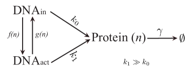
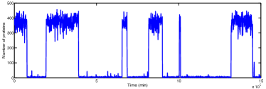
Figure 1: A typical fast-slow genetic switching model considered in systems biology. Left panel: Schematics of the chemical reaction schemes, where the switching rates $f(n),~{}g(n)$ are usually large. Right panel: Direct Monte Carlo simulations of the genetic switching model. The bi-stability is clearly observed from the time series of protein copy numbers.

The biologically relevant parameter setup is $\gamma\sim O(1)$ and $k_{0}/\gamma,~{}k_{1}/\gamma$ both large. We will not consider more detailed regimes concerning the magnitudes of $k_{1}$ and $k_{0}$ although one usually has $k_{1}\gg k_{0}$ in realistic situations. This does not affect the main point in this paper. In this case, the average number of proteins at steady state is of order $k_{1}/\gamma$. Now let us define the small parameter $\epsilon\approx\gamma/k_{1}$ or $\gamma/k_{0}$, thus the characteristic number of proteins is $n\sim O(\epsilon^{-1})$. In our fast-slow genetic switching model, we define the switching rates $f(n),g(n)\sim O(\epsilon^{-\alpha})$, and the realistic situations can be classified into the following three typical regimes:

• Case 1: $\alpha>1$, i.e. the genetic switching process is much faster than the translation process;

• Case 2: $\alpha=1$, i.e. the switching rates are comparable to the translation rates;

• Case 3: $0<\alpha<1$, i.e. the translation process is much faster than the genetic switching process.

In Case 2, the WKB asymptotics and the rigorous LDT results have been established for a similar model which takes into account the mRNA fluctuationLiLin . The obtained LDT rate functional is utilized to find the most probable transition path and characterize the rate of transitions between the high and low expression states. Furthermore, the authors have shown that the Hamiltonian obtained from LDT is convex with respect to the momentum variable, which is one key point in designing robust numerical algorithms. In Case 3, the researchers typically take the continuum limit to the translation process at first since it is even faster than the switching processGe . With this approach, one obtains a stochastic hybrid system which resembles similar form as those for ion channels considered in computational neuroscience. So far, the WKB asymptotics and path integral formulations are both proposed for stochastic hybrid systems. The Case 1 is also studied with WKB asymptotics applied to the averaged system with respect to the fast switching process.

From the authors’ point of view, the approaches employed in [Ge, ] are like taking a repeated limit to the switching and translation processes according to their relative magnitudes. More concretely, when DNA switching is much faster than the protein synthesis, the equilibrium pre-averaging of the switching process is taken in [Ge, ] at first and one gets a pure translation process with effective translation rates; however when the protein synthesis is much faster than DNA switching, the large volume limit is taken to the translation process at first and one gets a stochastic hybrid systemGe . Similar ideas and techniques are adopted in [Newby Phys Biol, ] and [Newby Math Biol, ] as well, which discussed different timescale issues for the gene expression model. With this understanding, it will be interesting to investigate the double limit of the original process instead of taking average with respect to one faster process at first. Mathematically it is also desirable to establish the large deviations for the original system with two time scales but different magnitudes. In fact, it is the main motivation of this paper. We will utilize the Doi-Peliti second quantization path integral formalism Doi ; Peliti ; Wang to study the general two-scale large deviations for the genetic switching models. As we will see, although the second quantization path integral for the spin-boson type model is formal, it is an effective approach to derive the large deviation results for chemical jump processes. Compared with the classical path integral formalism for diffusion processes, the second quantization path integral for chemical jump processes formulates the weight of each path in an extended space which involves both coordinate and momentum variables. This makes that the large deviation result can be given through a Hamiltonian with explicit formula, which resolves the dilemma that the Lagrangian in the rate functional does not have a closed form. This is important for further theoretical and numerical studies. Mathematically, rigorously establishing the LDT obtained from the formal approach in this paper is in progress based on our previous analysis [LiLin, ].

Let us briefly illustrate our general two-scale LDT results. We will show that the Lagrangian obtained from the second quantization path integral comprises of two parts, which correspond to the switching and translation processes, respectively. However, what we are interested in is the LDT only for the concentration of proteins. The different magnitudes of the switching and translation rates essentially lead to a singularly perturbed variational problem, which has different dominant terms and different scaling limits in the cases of $0<\alpha<1$ and $\alpha>1$. When $\alpha=1$, the Lagrangians from both parts contribute equally, and we get a result which combines the Donsker-Varadhan type LDT Varadhan for the occupation measure of DNA states and the large volume type LDT Shwartz1995 for the small noise perturbation altogether [LiLin, ]. As the LDT gives the sharpest characterization of the considered two-scale chemical kinetic system, we can obtain the deterministic mean field ODEs and the chemical Langevin approximation for the system based on the local analysis of the large deviation results Dembo . This corresponds to the law of large numbers (LLN) and the central limit theorem (CLT) for the process. We found that the three cases possess the same mean field ODEs. However, the chemical Langevin approximations for them are quite different. If $\alpha>1$, only the fluctuation from protein translation process survives. If $0<\alpha<1$, only the fluctuation from genetic switching process survives. And if $\alpha=1$, both fluctuations from protein translation and genetic switching processes contribute. Similar results are also valid for the single-molecule Michaelis-Menten kinetics Xie with slight modifications (c.f. Section V). Our study extends the insights about the chemical kinetic systems in the classical large volume limit, and the methodology we introduced here can be applied to other multiscale problems in many fields.

The rest of the paper is organized as follows. In Section II, we introduce the chemical master equation and apply the Doi-Peliti path integral formalism to the considered model. We then rescale the system with system size $\epsilon^{-1}$ and get the abstract LDT result based on singular perturbation analysis in Section III. In Section IV, we apply our abstract result to the two-state genetic switching model and present the mean field limits and chemical Langevin approximations. In Section V, we apply our result to the well-known single-molecule Michaelis-Menten kinetics and mention the implications. Finally we make the conclusion and related discussions in Section VI.

II Transition Probability in a Path Integral Form

We start from a more general model rather than Eq. (5). Assume that the DNA switching could occur among $N$ possible states ($N=2$ for the model shown in Fig. 1) and the chemical master equation (CME) for the biological reaction network reads

$$\frac{\partial}{\partial t}\boldsymbol{P}(n,t) = \boldsymbol{A}\Big{[}\boldsymbol{P}(n-1,t)-\boldsymbol{P}(n,t)\Big{]}$$

$$+\gamma\Big{[}(n+1)\boldsymbol{P}(n+1,t)-n\boldsymbol{P}(n,t)\Big{]}$$

$$+\boldsymbol{Q}^{\dagger}\boldsymbol{P}(n,t).$$

Here $\boldsymbol{P}(n,t)=(P_{1}(n,t),\ldots,P_{N}(n,t))^{T}$, $P_{j}(n,t)$ is the probability distribution function that the system has $n$ protein copy numbers and the switch is in state $j$ at time $t$. $\boldsymbol{A}$ is a diagonal matrix with diagonal entry $k_{j}$ as the protein synthesis rate in state $j$. $\gamma$ is the protein degradation rate and $\boldsymbol{Q}=(q_{jk}(n))_{j,k=1}^{N}$ is the transition rate matrix among different DNA states. Thus $q_{jk}(n)\geq 0$ for any $j\neq k$ and $\sum_{k=1}^{N}q_{jk}(n)=0$. We assume that the switching process is ergodic.

Now we follow the Doi-Peliti’s approach to establish the path integral formalism of the CME (II) Wolyness ; Wang ; Doi ; Peliti . Define the creation, annihilation operators $a^{\dagger},a$ and the state function $|\boldsymbol{\psi}\rangle$ as

$$a^{\dagger}\left|n\right\rangle=\left|n+1\right\rangle,\quad a\left|n\right\rangle=n\left|n-1\right\rangle\text{ and }\left|\boldsymbol{\psi}\right\rangle=\sum\nolimits_{n=0}^{\infty}\boldsymbol{P}(n,t)\left|n\right\rangle.$$

Then the CME (II) can be written in a second-quantized form

$${\partial}_{t}\left|\boldsymbol{\psi}\right\rangle=\boldsymbol{\Omega}\left|\boldsymbol{\psi}\right\rangle,$$ (7)

where the operator

$$\boldsymbol{\Omega}=\boldsymbol{A}(a^{\dagger}-1)+\gamma(a-a^{\dagger}a)+\hat{\boldsymbol{Q}}^{\dagger}$$ (8)

and $\hat{\boldsymbol{Q}}$ is obtained from $\boldsymbol{Q}$ by replacing the transition rates $q_{ij}(n)$ with operators $q_{ij}(a^{\dagger}a)$.

From Eq. (7), the transition probability $P(n_{f},\tau|n_{i},0)$ of finding product copy number $n_{f}$ at time $t=\tau$ starting from $n_{i}$ at $t=0$ has the form

$$P(n_{f},\tau|n_{i},0) = \left\langle{\boldsymbol{n}_{f}}\right|\exp(\boldsymbol{\Omega}\tau)\left|{\boldsymbol{n}_{i}}\right\rangle$$ (9)

$$= \mathop{\lim}\limits_{\Delta t\to 0}\left\langle{\boldsymbol{n}_{f}}\right|\exp(\boldsymbol{\Omega}\Delta t)^{\tau/\Delta t}\left|{\boldsymbol{n}_{i}}\right\rangle,$$

where $\left|{\boldsymbol{n}_{i}}\right\rangle=(\left|n_{i}\right\rangle,\left|n_{i}\right\rangle,\cdots,\left|n_{i}\right\rangle)^{T}$ is an $N$-dimensional column vector and $\left\langle{\boldsymbol{n}_{f}}\right|=(\left\langle{n_{f}}\right|,\cdots,\left\langle{n_{f}}\right|)$ is an $N$-dimensional row vector. Following Zhang et al. Wang , we utilize the coherent state representation and a resolution of identity Wolyness ; Wang as

$$\boldsymbol{I}_{b}\otimes\boldsymbol{I}_{s}=\int_{0}^{\infty}dn\int_{-\pi}^{\pi}\frac{d\beta}{2\pi}\left|z\right\rangle\left\langle{\tilde{z}}\right|e^{-n}\cdot\frac{1}{N^{N-2}}\prod\limits_{k=1}^{N-1}\int_{0}^{(N/2)\pi}\sin\frac{2\theta_{k}}{N}d\theta_{k}\frac{1}{4\pi}\int_{0}^{4\pi}d\phi_{k}|\boldsymbol{\psi}^{R}\rangle\langle\boldsymbol{\psi}^{L}|,$$ (10)

where

$$|{{\boldsymbol{\psi}^{R}}}\rangle=\left[\begin{matrix}{\frac{2}{N}{{\cos}^{2}}\frac{{{\theta_{1}}}}{N}e^{i\phi_{1}/2}}\\ \vdots\\ {\frac{2}{N}{{\cos}^{2}}\frac{{{\theta_{N}}}}{N}e^{i\phi_{N}/2}}\\ \end{matrix}\right],\quad\langle\boldsymbol{\psi}^{L}|=(e^{-i\phi_{1}/2},\cdots,e^{-i\phi_{N}/2})$$

with

$$\left|z\right\rangle=e^{a^{\dagger}z}\left|0\right\rangle,\ \left\langle{\tilde{z}}\right|=\left\langle 0\right|e^{a\tilde{z}},\ z=ne^{-i\beta},\ \tilde{z}=e^{i\beta},$$

and $i$ is the imaginary unit. The variable $n$ has the interpretation that it characterizes the mean protein number in the coherent states. Define $c_{j}=(2/N){{\cos}^{2}}({\theta_{j}/N})$. The $c_{j}$ gives the occupation probability of DNA at state $j$ from the probabilistic interpretation of quantum mechanics. They satisfy the normalization condition $\sum_{j=1}^{N}c_{j}=1$. Correspondingly the phase variable $\boldsymbol{\phi}$ can be chosen to satisfy $\sum_{j=1}^{N}\phi_{j}=0$ for convenience. These choices are consistent with the resolution of identity. As a consequence, we have only $N-1$ independent unknowns $(c_{1},\ldots,c_{N-1})$ in $\boldsymbol{c}=(c_{1},\ldots,c_{N})$, which is equivalent to use $\boldsymbol{\theta}=(\theta_{1},\ldots,\theta_{N})$, and $N-1$ unknowns $(\phi_{1},\ldots,\phi_{N-1})$ in $\boldsymbol{\phi}=(\phi_{1},\ldots,\phi_{N})$.

Inserting (10) into (9), the transition probability density can be represented as a path integral form

$$P(n_{f},\tau|n_{i},0)=\text{Const.}\times\int DnD\beta D\boldsymbol{c}D\boldsymbol{\phi}\exp\left(-\int_{0}^{\tau}Ldt\right),$$ (11)

where the Lagrangian $L$ is defined as

$$L=i\beta\frac{dn}{dt}+\sum_{j=1}^{N-1}i\phi_{j}\frac{d(c_{N}-c_{j})/2}{dt}-H(n,\boldsymbol{c},i\beta,i\boldsymbol{\phi}),$$ (12)

and the Hamiltonian

$$H(n,\boldsymbol{c},i\beta,i\boldsymbol{\phi})=H_{1}(n,\boldsymbol{c},i\beta)+H_{2}(n,\boldsymbol{c},i\boldsymbol{\phi})$$ (13)

with $H_{1}$ for the translation process

$$H_{1}(n,\boldsymbol{c},i\beta)=\sum_{j=1}^{N}k_{j}c_{j}[\exp(i\beta)-1]+\gamma n[\exp(-i\beta)-1]$$ (14)

and $H_{2}$ for the switching process

$$H_{2}(n,\boldsymbol{c},i\boldsymbol{\phi})=\sum_{m,j}^{N}c_{m}q_{mj}(n)(e^{(i\phi_{m}-i\phi_{j})/2}-1).$$ (15)

In Eq. (11), the outer 4-fold integral is taken in the path space with respect to $n(t),\beta(t),\boldsymbol{c}(t)$ and $\boldsymbol{\phi}(t)$, which are full trajectories in $[0,\tau]$. The terms involving $|n_{i}\rangle$ and $\langle n_{f}|$ have been absorbed to the constant before the integral. The path integral formulation (11) makes the weight of each trajectory explicit. The form of Lagrangian (12) suggests the interpretation that the pairs $i\beta$ and $n$, $i\phi$ and $c$ are conjugate variables.

To study the associated LDT, we must have a small parameter $\epsilon$ and a deterministic limit as $\epsilon\rightarrow 0$. This could be chosen as the inverse of typical system size $\epsilon=\gamma/k_{1}=V^{-1}$. As stated in the introduction section, we assume

$$k_{j}\sim\frac{1}{\epsilon},\quad q_{ij}\sim\frac{1}{\epsilon^{\alpha}},\quad\alpha>0$$ (16)

and define

$$x=n\epsilon,\quad\tilde{k}_{j}=k_{j}\epsilon,\quad\tilde{q}_{jk}(x)=q_{jk}(n)\epsilon^{\alpha}.$$ (17)

With these definitions, Eq. (11) can be rewritten as

$$P(n_{f},\tau|n_{i},0)=\text{Const.}\times\int DxD\beta D\boldsymbol{c}D\boldsymbol{\phi}\exp\left(-\frac{1}{\epsilon}\int_{0}^{\tau}\tilde{L}_{1}dt-\frac{1}{\epsilon^{\alpha}}\int_{0}^{\tau}\tilde{L}_{2}dt\right),$$ (18)

where the rescaled Lagrangian

$$\tilde{L}_{1}=i\beta\frac{dx}{dt}-\tilde{H}_{1}(x,\boldsymbol{c},i\beta),$$ (19)

$$\tilde{L}_{2}=\epsilon^{\alpha}\sum_{j=1}^{N-1}i\phi_{j}\frac{d(c_{N}-c_{j})/2}{dt}-\tilde{H}_{2}(x,\boldsymbol{c},i\boldsymbol{\phi}),$$ (20)

and rescaled Hamiltonian

$$\tilde{H}_{1}(x,\boldsymbol{c},i\beta)=\sum_{j=1}^{N}\tilde{k}_{j}c_{j}[\exp(i\beta)-1]+\gamma x[\exp(-i\beta)-1],$$ (21)

$$\tilde{H}_{2}(x,\boldsymbol{c},i\boldsymbol{\phi})=\sum_{m,j}^{N}c_{m}\tilde{q}_{mj}(x)(e^{(i\phi_{m}-i\phi_{j})/2}-1).$$ (22)

Using the method of steepest descent asymptotics, the integration over $\beta$ and $\boldsymbol{\phi}$ can be approximated by simply using the value of the integrand at the saddle point Orszag . Thus, we get

$$P(n_{f},\tau|n_{i},0)\propto\int DxD\boldsymbol{c}\exp\left(-\frac{1}{\epsilon}\int_{0}^{\tau}L_{1}(x,\dot{x},\boldsymbol{c})dt-\frac{1}{\epsilon^{\alpha}}\int_{0}^{\tau}L_{2}(x,\boldsymbol{c})dt\right),$$ (23)

where

$$L_{1}(x,\dot{x},\boldsymbol{c}) = \mathop{\sup}_{p}\{p\dot{x}-\tilde{H}_{1}(x,\boldsymbol{c},p)\},$$ (24)

$$L_{2}(x,\boldsymbol{c}) = \mathop{\sup}_{\boldsymbol{\varphi}}\{-\tilde{H}_{2}(x,\boldsymbol{c},\boldsymbol{\varphi})\}.$$ (25)

Note the term $\boldsymbol{\varphi}\cdot\dot{\boldsymbol{c}}$ does not appear in Eq. (25) because of the factor $\epsilon^{\alpha}$ in the first term of Eq. (20). Formally, the functional appearing in the exponential in (23) is a competition between the rate functional $\int L_{1}dt$ which corresponding to the translation process and the rate functional $\int L_{2}dt$ which corresponding to the switching process. It is interesting to observe that the Lagrangian $L_{1}$ corresponds to the large volume type LDT rate function for the small noise perturbation Shwartz1995 and $L_{2}$ corresponds to the Donsker-Varadhan type LDT rate function for the occupation measure of DNA states Shwartz1995 ; Varadhan . The second quantization path integral perfectly reveals the intrinsic structure of the considered two-scale chemical kinetic process.

III Formulation of the LDT in a general setting

The transition probability (23) contains the LDT information about the variables $x$ and $\boldsymbol{c}$. However in most cases, one is only interested in slow variables, i.e. the concentration of protein in our case, which is also the observable in experiments. In this sense, we must integrate over $\boldsymbol{c}$-space. It turns out the final result depends on the value of $\alpha$ and we will have three typical regimes. In what follows, we will discuss different outcomes in different regimes separately.

(i). Case 1: $\alpha>1$. The switching process is much faster than the translation process.

In this case, we can rewrite Eq. (23) as

$$P(n_{f},\tau|n_{i},0)\propto\int DxD\boldsymbol{c}\exp\left\{-\frac{1}{\epsilon}\int_{0}^{\tau}dt\left(L_{1}(x,\dot{x},\boldsymbol{c})+\frac{1}{\epsilon^{\alpha-1}}L_{2}(x,\boldsymbol{c})\right)\right\}.$$ (26)

To integrate over $\boldsymbol{c}$-space, we take the Laplace asymptotics for each $t$. The Lagrangian for $x$ has the form

$$L_{x}(x,\dot{x})=\mathop{\inf}_{\boldsymbol{c}}\left\{L_{1}(x,\dot{x},\boldsymbol{c})+\frac{1}{\epsilon^{\alpha-1}}L_{2}(x,\boldsymbol{c})\right\}\quad\text{as}\quad\epsilon\rightarrow 0+.$$ (27)

Since $L_{2}\geq 0$ and $\epsilon^{1-\alpha}\gg 1$, the term $\epsilon^{1-\alpha}L_{2}(x,\boldsymbol{c})$ dominates. From the assumption that the switching process is ergodic, for a given $x$, $L_{2}(x,\boldsymbol{c})$ achieves its minimum $L_{2}(x,\boldsymbol{c})=0$ at a single point $\boldsymbol{c}=\boldsymbol{c}_{0}(x)$, i.e. the steady state distribution given the concentration $x$ Shwartz1995 ; Kemeny . Thus we get

$$L_{x}(x,\dot{x}) = L_{1}(x,\dot{x},\boldsymbol{c}_{0}(x))$$ (28)

and

$$P(n_{f},\tau|n_{i},0)\propto\int Dx\exp\left\{{-\frac{1}{\epsilon}\int_{0}^{\tau}dtL_{x}(x,\dot{x})}\right\}.$$ (29)

Although we still leave the factor $\epsilon^{1-\alpha}$ in the Laplace aysmptotics (27) in our manipulation and then take the singular perturbation analysis, it is not difficult to establish the final result in a rigorous way. This result tells us that when $\alpha>1$ the LDT for the slow variable $x$ is only determined by the effective synthesis rate $\sum_{j=1}^{N}\tilde{k}_{j}({\boldsymbol{c}}_{0}(x))_{j}$ and degradation rate $\gamma$.

(ii). Case 3: $0<\alpha<1$. The translation process is much faster than the switching process.

In this case, we rewrite Eq. (23) as

$$P(n_{f},\tau|n_{i},0)\propto\int DxD\boldsymbol{c}\exp\left\{-\frac{1}{\epsilon^{\alpha}}\int dt\left(\frac{1}{\epsilon^{1-\alpha}}L_{1}(x,\dot{x},\boldsymbol{c})+L_{2}(x,\boldsymbol{c})\right)\right\}.$$ (30)

Taking Laplace asymptotics with respect to $\boldsymbol{c}$-integral, we get

$$L_{x}(x,\dot{x})=\mathop{\inf}_{\boldsymbol{c}}\left(\frac{1}{\epsilon^{1-\alpha}}L_{1}(x,\dot{x},\boldsymbol{c})+L_{2}(x,\boldsymbol{c})\right).$$ (31)

Since $L_{1}\geq 0$ and $\epsilon^{\alpha-1}\gg 1$, the term $\epsilon^{\alpha-1}L_{1}(x,\dot{x},\boldsymbol{c})$ dominates. We can perform similar approach to derive $L_{x}$ as in the previous case. In general, we assume that $L_{1}(x,\dot{x},\boldsymbol{c})$ achieves its minimum $L_{1}(x,\dot{x},\boldsymbol{c})=0$ at $\boldsymbol{c}=\boldsymbol{c}_{x}$ for a given $x$. In our case, $\boldsymbol{c}_{x}$ satisfies the mean field ODE by large volume limit:

$$\dot{x}=\sum_{j=1}^{N}k_{j}(\boldsymbol{c}_{x})_{j}-\gamma x.$$ (32)

By (31) and (32), we have

$$L_{x}(x,\dot{x})=\mathop{\inf}_{\{\boldsymbol{c}_{x}:\dot{x}=\sum_{j=1}^{N}k_{j}(\boldsymbol{c}_{x})_{j}-\gamma x\}}L_{2}(x,\boldsymbol{c}_{x})$$ (33)

and

$$P(n_{f},\tau|n_{i},0)\propto\int Dx\exp\left\{{-\frac{1}{\epsilon^{\alpha}}\int_{0}^{\tau}dtL_{x}(x,\dot{x})}\right\}.$$ (34)

We want to remark here that from (34) we will expect to get the LDT of the type

$$\lim_{\epsilon\rightarrow 0+}\epsilon^{\alpha}\ln\text{Prob}(X_{\cdot}\in\mathcal{B})=-\inf_{x\in\mathcal{B}}\int_{0}^{\tau}L_{x}(x,\dot{x})dt$$ (35)

where $\mathcal{B}$ is a Borel set in $D[0,\tau]$ space (functions on $[0,\tau]$ are right continuous with left limits) and $X_{\cdot}$ is the sample path of the original jump process. The scaling $\epsilon^{\alpha}$ in (35) is essential to reveal the nontrivial behavior of $x$. Other choices of the exponent do not give the correct limit which we are interested in for $x$.

In the considered case $0<\alpha<1$, the protein synthesis are much faster than the genetic switching. With this condition, if we neglect the copy-number fluctuation of the protein, we get a reduced stochastic hybrid system:

$$\dot{x}=\sum_{j=1}^{N}k_{j}I_{\{\xi(t)=j\}}-\gamma x,$$ (36)

where $I_{\{\xi(t)=j\}}$ is an indicator function and $\xi(t)$ represents the DNA occupation state. In [Bressloff, ] and [FAGGIONATO, ], the authors established the LDTs for variable $x$ as $\epsilon\to 0+$ for the system (36), which is the same as what we derived in Eq. (33). But we should emphasize that this coincidence is not obvious a priori, our result supports the validity of the procedure by taking the repeated limit for two-scale processes in some sense.

(iii). Case 2: $\alpha=1$. The switching rates are comparable to the translation rates.

When $\alpha=1$, we have

$$P(n_{f},\tau|n_{i},0)=\int DxD\boldsymbol{c}\exp\left\{-\frac{1}{\epsilon}\left(\int dtL_{1}(x,\dot{x},\boldsymbol{c})+\int dtL_{2}(x,\boldsymbol{c})\right)\right\}.$$ (37)

In this case, we have the LDT Lagrangian for variable $x$:

$$L_{x}(x,\dot{x})=\mathop{\inf}_{\boldsymbol{c}}\left\{L_{1}(x,\dot{x},\boldsymbol{c})+L_{2}(x,\boldsymbol{c})\right\}.$$ (38)

Since in most cases there is no closed form for $L_{1}$, thus we do not expect to get the closed form of $L_{x}$ accordingly. This hinders the applicability of the obtained theory. It is more convenient to study the conjugate Hamiltonian of $L_{x}$:

$$H_{x}(x,p) = \mathop{\sup}_{\beta}\left\{p\beta-L_{x}(x,\beta)\right\}$$ (39)

$$= \mathop{\sup}_{\beta}\left\{p\beta-\mathop{\inf}_{\boldsymbol{c}}\left\{L_{1}(x,\beta,\boldsymbol{c})+L_{2}(x,\boldsymbol{c})\right\}\right\}$$

$$= \mathop{\sup}_{\beta}\mathop{\sup}_{\boldsymbol{c}}\left\{p\beta-L_{1}(x,\beta,\boldsymbol{c})-L_{2}(x,\boldsymbol{c})\right\}$$

$$= \mathop{\sup}_{\boldsymbol{c}}\mathop{\sup}_{\beta}\left\{p\beta-L_{1}(x,\beta,\boldsymbol{c})-L_{2}(x,\boldsymbol{c})\right\}$$

$$= \mathop{\sup}_{\boldsymbol{c}}\left\{\tilde{H}_{1}(x,p,\boldsymbol{c})-L_{2}(x,\boldsymbol{c})\right\}.$$

As we will show, the dual Hamiltonian may have explicit expression and it is convex with respect to the momentum variable $p$. This property makes it competitive for the numerical algorithms for solving static Hamilton-Jacobi equation through the geometric minimum action method (gMAM)gMAM ; Lv14 .

IV Application to the two-state model

Using the two-state model (5) as an example, we will give the detailed LDT results for different $\alpha$, and show the mean field ODE and the chemical Langevin approximation for variable $x$. Moreover, we will solve the static Hamilton-Jacobi equation for the quasi-potential $\Phi(x)$ in different situations. At first, we take the same rescaling (17) for the variables and parameters. We again consider three different cases: (i) $\alpha>1$, (ii) $0<\alpha<1$ and (iii) $\alpha=1$.

(i). Case 1: $\alpha>1$.

In this case, the ergodic limit of DNA occupation probability is

$$\boldsymbol{c}_{0}(x)=\left(\frac{\tilde{f}(x)}{\tilde{f}(x)+\tilde{g}(x)},~{}\frac{\tilde{g}(x)}{\tilde{f}(x)+\tilde{g}(x)}\right)$$

for given $x$. By Eq. (27), we have

$$L_{x}(x,\dot{x})=\mathop{\sup}_{p}\left\{p\dot{x}-\left[\frac{\tilde{k}_{1}\tilde{f}(x)+\tilde{k}_{0}\tilde{g}(x)}{\tilde{f}(x)+\tilde{g}(x)}(\exp(p)-1)+\gamma x(\exp(-p)-1)\right]\right\},$$ (40)

and the dual Hamiltonian

$$H_{x}(x,p)=\frac{\tilde{k}_{1}\tilde{f}(x)+\tilde{k}_{0}\tilde{g}(x)}{\tilde{f}(x)+\tilde{g}(x)}[\exp(p)-1]+\gamma x[\exp(-p)-1].$$ (41)

From the result

$$\frac{\partial H_{x}}{\partial p}\Big{|}_{p=0}=\frac{\tilde{k}_{1}\tilde{f}(x)+\tilde{k}_{0}g(x)}{\tilde{f}(x)+\tilde{g}(x)}-\gamma x,$$ (42)

we get the mean field ODE

$$\frac{dx}{dt}=\frac{\partial H_{x}}{\partial p}\Big{|}_{p=0}=\frac{\tilde{k}_{1}\tilde{f}(x)+\tilde{k}_{0}\tilde{g}(x)}{\tilde{f}(x)+\tilde{g}(x)}-\gamma x.$$ (43)

Furthermore, the fact

$$\frac{\partial^{2}H_{x}}{\partial p^{2}}\Big{|}_{p=0}=\frac{\tilde{k}_{1}\tilde{f}(x)+\tilde{k}_{0}\tilde{g}(x)}{\tilde{f}(x)+\tilde{g}(x)}+\gamma x$$ (44)

shows the following chemical Langevin approximation holds

$$dx=\left(\frac{\tilde{k}_{1}f(x)+\tilde{k}_{0}\tilde{g}(x)}{\tilde{f}(x)+\tilde{g}(x)}-\gamma x\right)dt+\sqrt{\epsilon}\left(\sqrt{\frac{\tilde{k}_{1}\tilde{f}(x)+\tilde{k}_{0}\tilde{g}(x)}{\tilde{f}(x)+\tilde{g}(x)}}dw_{1}-\sqrt{\gamma x}dw_{2}\right),$$ (45)

where $w_{1}$ and $w_{2}$ are independent standard Brownian motions.

From classical variational analysis Rockafellar , it can be shown that the quasi-potential defined through

$$\Phi(x;x_{0})=\inf_{\tau\geq 0}\inf_{x(0)=x_{0},x(\tau)=x}\int_{0}^{\tau}L_{x}(x,\dot{x})dt$$

in our case satisfies a static Hamilton-Jacobi equation $H(x,\partial_{x}\Phi)=0$, where $x_{0}$ is a stable fixed point. Based on (41), we have by some algebra

$$\partial_{x}\Phi=-\log\frac{(\tilde{k}_{1}\tilde{f}(x)+\tilde{k}_{0}\tilde{g}(x))/(\tilde{f}(x)+\tilde{g}(x))}{\gamma x}.$$ (46)

This result is consistent with the quasi-potential derived in [Ge, ], where the authors neglect the fluctuation of genetic switching and get the result by WKB ansatz. But of course, there is no hope to get the explicit formula of $\Phi$ when the dimension of $x$ is bigger than 1.

(ii). Case 3: $0<\alpha<1$.

In this case, we have the Lagrangian

$$L_{x}(x,\dot{x}) = L_{2}(x,\boldsymbol{c}_{x})$$ (47)

$$= \mathop{\sup}_{\varphi}\left\{-\left[c_{1}\tilde{g}(x)(e^{\phi_{1}-\phi_{2}}-1)+c_{2}\tilde{f}(x)(e^{\phi_{2}-\phi_{1}}-1)\right]\right\}$$

$$= \left(\sqrt{\tilde{f}(x)c_{2}}-\sqrt{\tilde{g}(x)c_{1}}\right)^{2},$$

where $\boldsymbol{c}_{x}=(c_{1},c_{2})$ and $c_{1}=(\dot{x}-\tilde{k}_{0}+\gamma x)/(\tilde{k}_{1}-\tilde{k}_{0})$, $c_{2}=1-c_{1}$ by the condition $L_{1}(x,\dot{x},\boldsymbol{c}_{x})=0$. With the Legendre-Fenchel transform defined by $H_{x}(x,p)=\mathop{\sup}_{\beta}\left(p\beta-L_{x}(x,\beta)\right)$, we get the dual Hamiltonian:

$$H_{x}(x,p)=p\beta_{0}-L_{x}(x,\beta_{0}),$$ (48)

where $\beta_{0}=\tilde{k}_{1}s_{1}+\tilde{k}_{2}(1-s_{1})-\gamma x$ and

$$s_{1}=\frac{1}{2}+\frac{s_{2}}{2\sqrt{s_{2}^{2}+4}},\quad s_{2}=\frac{p(\tilde{k}_{1}-\tilde{k}_{0})+\tilde{f}(x)-\tilde{g}(x)}{\sqrt{\tilde{f}(x)\tilde{g}(x)}}.$$

Again, we can obtain the deterministic mean field ODE as

$$\frac{dx}{dt}=\frac{\partial H_{x}}{\partial p}\Big{|}_{p=0}=\frac{\tilde{k}_{1}\tilde{f}(x)+\tilde{k}_{0}\tilde{g}(x)}{\tilde{f}(x)+\tilde{g}(x)}-\gamma x.$$ (49)

Similarly, we get

$$\frac{\partial^{2}H_{x}}{\partial p^{2}}\Big{|}_{p=0}=\frac{2\tilde{f}(x)\tilde{g}(x)}{(\tilde{f}(x)+\tilde{g}(x))^{3}}(\tilde{k}_{1}-\tilde{k}_{0})^{2}$$ (50)

and thus the chemical Langevin approximation

$$dx=\left(\frac{\tilde{k}_{1}\tilde{f}(x)+\tilde{k}_{0}\tilde{g}(x)}{\tilde{f}(x)+\tilde{g}(x)}-\gamma x\right)dt+\sqrt{\epsilon^{\alpha}}\sqrt{\frac{2\tilde{f}(x)\tilde{g}(x)}{(\tilde{f}(x)+\tilde{g}(x))^{3}}(\tilde{k}_{1}-\tilde{k}_{0})^{2}}dw.$$ (51)

We note here that the fluctuation term has the strength $\sqrt{\epsilon^{\alpha}}$ since it originates from the fast genetic switching process, and the term $\sqrt{\gamma x}dw_{2}$ disappears because it is in order $\sqrt{\epsilon}$. These are in sharp contrast with the result in (45) and Case 2 below which has the $O(\sqrt{\epsilon})$ fluctuation.

By Eq. (48), solving the Hamilton-Jacobi equation $H(x,\partial_{x}\Phi)=0$, we have

$$\partial_{x}\Phi=\frac{\tilde{f}}{\tilde{k}_{0}-\gamma x}+\frac{\tilde{g}}{\tilde{k}_{1}-\gamma x}.$$ (52)

This is consistent with the result in [Ge, ] although we have totally different form of Hamiltonian $H$.

(iii). Case 2: $\alpha=1$.

In this case, the genetic switching rate is comparable to the protein synthesis rate. The rigorous LDT result has been obtained in [LiLin, ]. Now we formally establish the LDT again through the second-quantization path integral approach.

By (38) and (39), we have the dual Hamilton:

$$H_{x}(x,p) = \mathop{\sup}_{\boldsymbol{c}}\left\{\tilde{H}_{1}(x,\boldsymbol{c},p)-L_{2}(x,\boldsymbol{c})\right\}$$ (53)

$$= \mathop{\sup}_{\boldsymbol{c}}\bigg{\{}\left(\tilde{k}_{1}c_{1}+\tilde{k}_{0}c_{2}\right)[\exp(p)-1]+\gamma x[\exp(-p)-1]-\left(\sqrt{(\tilde{f}(x)c_{2}}-\sqrt{\tilde{g}(x)c_{1}}\right)^{2}\bigg{\}}.$$

Since $c_{1}+c_{2}=1$ and $c_{j}\geq 0$, we can obtain the explicit expression of $H_{x}(x,p)$:

$$H_{x}(x,p) = \left(\tilde{k}_{1}s+\tilde{k}_{0}(1-s)\right)[\exp(p)-1]+\gamma x[\exp(-p)-1]-\left(\sqrt{(\tilde{f}(1-s)}-\sqrt{\tilde{g}s}\right)^{2}.$$ (54)

where

$$s=\frac{1}{2}+\frac{s_{1}}{2\sqrt{s_{1}^{2}+4}},\quad s_{1}=\frac{(\tilde{k}_{1}-\tilde{k}_{0})(e^{p}-1)+\tilde{f}(x)-\tilde{g}(x)}{\sqrt{\tilde{f}(x)\tilde{g}(x)}}.$$

As before, we get the mean field ODE

$$\frac{dx}{dt}=\frac{\partial H_{x}}{\partial p}\Big{|}_{p=0}=\frac{\tilde{k}_{1}\tilde{f}(x)+\tilde{k}_{0}\tilde{g}(x)}{\tilde{f}(x)+\tilde{g}(x)}-\gamma x.$$ (55)

The second order expansion to $p$

$$\frac{\partial^{2}H_{x}}{\partial p^{2}}\Big{|}_{p=0}=\frac{2\tilde{f}(x)\tilde{g}(x)}{(\tilde{f}(x)+\tilde{g}(x))^{3}}(\tilde{k}_{1}-\tilde{k}_{0})^{2}+\frac{\tilde{k}_{1}\tilde{f}(x)+\tilde{k}_{0}\tilde{g}(x)}{\tilde{f}(x)+\tilde{g}(x)}+\gamma x$$ (56)

yields the following chemical Langevin approximation

$$dx = \left(\frac{\tilde{k}_{1}\tilde{f}+\tilde{k}_{0}\tilde{g}}{\tilde{f}+\tilde{g}}-\gamma x\right)dt+\sqrt{\epsilon}\left(\sqrt{\frac{\tilde{k}_{1}\tilde{f}+\tilde{k}_{0}\tilde{g}}{\tilde{f}+\tilde{g}}+\frac{2\tilde{f}\tilde{g}}{(\tilde{f}+\tilde{g})^{3}}(\tilde{k}_{1}-\tilde{k}_{0})^{2}}dw_{1}-\sqrt{\gamma x}dw_{2}\right).$$ (57)

where $\tilde{f},\tilde{g}$ are abbreviations of $\tilde{f}(x)$ and $\tilde{g}(x)$, and $w_{1},w_{2}$ are independent standard Brownian motions.

It is worth discussing the relationship between the Hamiltonian (54) and that obtained by WKB asymptotics. To get a Hamiltonian via WKB asymptotics, we follow the procedures in [Newby Dyn Syst, ] and sketch its outline. We assume that the stationary solution of (II) has the form

$$P_{i}^{s}(x)\sim r_{i}(x)k(x)\exp\left[-\frac{1}{\epsilon}\Phi(x)\right],\quad i=1,2.$$ (58)

Substituting (58) into (II) and collecting leading order terms, we get $M(x,p)\cdot(r_{1}(x),r_{2}(x))^{T}=0$, where

$$M(x,p)=\left(\begin{array}[]{cc}\tilde{k}_{1}(e^{p}-1)+\gamma x(e^{-p}-1)-\tilde{g}&\tilde{f}\\ \tilde{g}&\tilde{k}_{0}(e^{p}-1)+\gamma x(e^{-p}-1)-\tilde{f}\end{array}\right).$$

Now there is a subtlety to get the correct Hamilton in LDT. If one takes the choice that the $H(x,p)$ is defined as the largest eigenvalue of $M(x,p)$, it can be shown that it is equivalent to (54). However if one takes another choice that it is defined as the determinant of $M(x,p)$ Newby Dyn Syst ; Assaf , then $H$ is not convex in momentum variable $p$ and the equivalence is lost. This resembles the issue of the choice of Hamiltonians for parametrized curve problem in classical mechanics (see p. 40 in [Buhler, ]).

Let us make some comments on the obtained mean-field limit and Langevin approximations. Recall that there are two parts of noise in the original dynamics: one is from the translation process and the other from DNA switching process. Our result tells that different diffusion approximations arise according to the magnitudes of residual noise in different reaction channels. If $\alpha>1$, the dominant part of noise is from the translation, so only the fluctuation from translation process survives. If $0<\alpha<1$, the dominant part is from switching process, so only the fluctuation from DNA switching process survives. And if $\alpha=1$, both fluctuations from protein translation and genetic switching contribute. Similar situation occurs in the LDT analysis, where the singular perturbation is performed for variational minimizations. The obtained results show the validity of the procedure by taking the limit for faster process at first and then performing the corresponding analysis for slower process. Although we only consider the two-state models, the essential structure and results hold for general cases. It is a natural extension of the classical large volume limit for chemical reaction processes. We summarize our discussions for the three regimes in Table 1.

Table 1: Comparison of LDTs, mean-field limits and Langevin approximations for three regimes

				LDT Hamiltonian	Deterministic Drift	Noise in Langevin Approximation
Case 1: ($\alpha>1$)	$H_{x}(x,p)$ in (41)	$\displaystyle\frac{\tilde{k}_{1}\tilde{f}(x)+\tilde{k}_{0}\tilde{g}(x)}{\tilde{f}(x)+\tilde{g}(x)}-\gamma x$	$\displaystyle\sqrt{\epsilon}\left(\sqrt{\frac{\tilde{k}_{1}\tilde{f}+\tilde{k}_{0}\tilde{g}}{\tilde{f}+\tilde{g}}}dw_{1}-\sqrt{\gamma x}dw_{2}\right)$
Case 2: ($\alpha=1$)	$H_{x}(x,p)$ in (54)		$\displaystyle\sqrt{\epsilon}\left(\sqrt{\frac{\tilde{k}_{1}\tilde{f}+\tilde{k}_{0}\tilde{g}}{\tilde{f}+\tilde{g}}+\frac{2\tilde{f}\tilde{g}}{(\tilde{f}+\tilde{g})^{3}}(\tilde{k}_{1}-\tilde{k}_{0})^{2}}dw_{1}-\sqrt{\gamma x}dw_{2}\right)$
Case 3: ($\alpha<1$)	$H_{x}(x,p)$ in (48)		$\displaystyle\sqrt{\epsilon^{\alpha}}\sqrt{\frac{2\tilde{f}\tilde{g}}{(\tilde{f}+\tilde{g})^{3}}(\tilde{k}_{1}-\tilde{k}_{0})^{2}}dw_{1}$

V Application to the Single-Molecule Michaelis-Menten kinetics

Our approach and observation have interesting implications on the single-molecule Michaelis-Menten system Xie , in which a substrate S binds reversibly with an enzyme E to form an enzyme-substrate complex ES that decomposes to form a product P. The reaction schemes can be schematically shown as

$$\begin{array}[]{ccccc}{\rm E+S}&\autorightleftharpoons{$k_1$}{$k_{-1}$}&${{\rm ES}}$&\autorightarrow{$k_2${}}&${{\rm E+P}}$,\end{array}\quad\quad\begin{array}[]{ccc}{\rm P}&\autorightarrow{${\tiny\gamma}${}}&\emptyset.\end{array}$$ (61)

In case of single-molecule enzyme set-up, the reaction system (61) falls in the framework considered in this paper. As in [Xie, ], we assume that the substrate is abundant enough and there is essentially no depletion of substrate by a single enzyme molecule. That is, we assume the concentration of substrate is a constant, which will be denoted as $[S]$. It is well-known that the rate of product formulation $v$ has the following form in the quasi-steady state approximation Keener

$$v=\frac{k_{2}[S]}{[S]+k_{M}},$$ (62)

where $k_{M}=(k_{-1}+k_{2})/k_{1}$. In [Xie, ], the statistics of enzymatic turn-over time and dynamical disorder are considered. Here we are interested in deriving the Langevin approximations of the Michaelis-Menten system in different regimes.

In [Xie, ], $k_{-1}$ ranges from $0s^{-1}$ to $2000s^{-1}$, $k_{1}$ is usually taken as $10^{7}M^{-1}s^{-1}$, $k_{2}=250s^{-1}$, and $[S]$ ranges from the order $0.001mM$ to $0.1mM$, where $1M=1\text{mol/L}$. Some specific choices of these parameters include

• Case 1: $k_{-1}=2000s^{-1},k_{1}[S]=10^{7}M^{-1}s^{-1}\times 0.30mM=3000s^{-1},k_{2}=250s^{-1};$

• Case 2: $k_{-1}=200s^{-1},k_{1}[S]=10^{7}M^{-1}s^{-1}\times 0.02mM=200s^{-1},k_{2}=250s^{-1};$

• Case 3: $k_{-1}=50s^{-1},k_{1}[S]=10^{7}M^{-1}s^{-1}\times 0.005mM=50s^{-1},k_{2}=250s^{-1}.$

The degradation rate constant $\gamma$ is not essential and we assume it is $O(1s^{-1})$. The above choices underlie the rationale to study different regimes in previous sections since we can make the assumption

$$k_{2}\sim\frac{1}{\epsilon},\quad k_{1}[S],k_{-1}\sim\frac{1}{\epsilon^{\alpha}},\quad\alpha>0$$ (63)

if we define $\epsilon=1/250$.

The chemical master equation of the system (61) can be written as

$${\partial_{t}}\boldsymbol{P}(n,t) = \left(\begin{array}[]{cc}0&k_{2}\\ 0&0\end{array}\right)(\mathbb{E}_{n}^{-1}-1)\boldsymbol{P}(n,t)+\gamma(\mathbb{E}_{n}^{1}-1)[n\boldsymbol{P}(n,t)]+\left({\begin{array}[]{cc}{-k_{1}[S]}&{k_{-1}+k_{2}}\\ {k_{1}[S]}&{-(k_{-1}+k_{2})}\\ \end{array}}\right)\boldsymbol{P}(n,t).$$ (68)

Denote $c_{1}$ the occupation probability of the free enzyme molecule state E and $c_{2}$ the probability of the complex state ES. With similar approach in deriving (11), the transition probability can be obtained with Lagrangian $L$

$$L=i\beta\frac{dn}{dt}+i\phi_{1}\frac{d(-c_{1})}{dt}-H(n,\boldsymbol{c},i\beta,i\boldsymbol{\phi}),$$ (69)

where the Hamiltonian

$$H(n,\boldsymbol{c},i\beta,i\boldsymbol{\phi})=k_{2}c_{2}[\exp(i\beta)-1]+\gamma n[\exp(-i\beta)-1]+c_{2}(k_{-1}+k_{2}e^{i\beta})(e^{i\phi_{2}}-1)+c_{1}k_{1}[S](e^{-i\phi_{2}}-1).$$ (70)

According to (63), we make the rescaling

$$x=n\epsilon\ (\text{or}\ x_{\alpha}=n\epsilon^{\alpha}),\quad\tilde{k}_{2}=k_{2}{\epsilon},\quad\tilde{k}_{1}=k_{1}[S]{\epsilon^{\alpha}},\quad\tilde{k}_{-1}=k_{-1}{\epsilon^{\alpha}}.$$ (71)

Then the Cases 1, 2 and 3 correspond to $\alpha>1$, $\alpha=1$ and $0<\alpha<1$, respectively. Next let us study the three cases separately. The order of discussion will be from easy to difficult, which may be slightly different from previous sections.

(i). Case 2: $\alpha=1$.

With the steepest descent asymptotics as in (23), we have

$$P(n_{f},\tau|n_{i},0)\propto\int DxD\boldsymbol{c}\exp\left(-\frac{1}{\epsilon}\int_{0}^{\tau}L(x,\dot{x},\boldsymbol{c})dt\right).$$ (72)

The Lagrangian $L$ has the form

$$L(x,\dot{x},\boldsymbol{c}) = \mathop{\sup}_{p}\mathop{\sup}_{\varphi}\{p\dot{x}-\tilde{H}(x,\boldsymbol{c},p,\varphi)\}$$ (73)

$$= \mathop{\sup}_{p}\{p\dot{x}-H(x,\boldsymbol{c},p)\},$$

where $H(x,\boldsymbol{c},p)=\inf_{\varphi}\{\tilde{H}(x,\boldsymbol{c},p,\varphi)\}$ and

$$\tilde{H}(x,\boldsymbol{c},p,\varphi)=\tilde{k}_{2}c_{2}(e^{p}-1)+\gamma x(e^{-p}-1)+c_{2}(\tilde{k}_{-1}+\tilde{k}_{2}e^{p})(e^{\varphi}-1)+c_{1}\tilde{k}_{1}(e^{-\varphi}-1).$$ (74)

In this case, we have the LDT Lagragian for variable $x$ by applying Laplace asymptotics

$$L_{x}(x,\dot{x})=\mathop{\inf}_{\boldsymbol{c}}\left\{L(x,\dot{x},\boldsymbol{c})\right\}.$$ (75)

Following the approaches in deriving (39), we get the conjugate Hamiltonian of $L_{x}$:

$$H_{x}(x,p) = \mathop{\sup}_{\beta}\left\{p\beta-L_{x}(x,\beta)\right\}=\mathop{\sup}_{\beta}\left\{p\beta-\mathop{\inf}_{\boldsymbol{c}}\left\{L(x,\beta,\boldsymbol{c})\right\}\right\}$$ (76)

$$= \mathop{\sup}_{\beta}\mathop{\sup}_{\boldsymbol{c}}\left\{p\beta-L(x,\beta,\boldsymbol{c})\right\}=\mathop{\sup}_{\boldsymbol{c}}\mathop{\sup}_{\beta}\left\{p\beta-L(x,\beta,\boldsymbol{c})\right\}$$

$$= \mathop{\sup}_{\boldsymbol{c}}\left\{H(x,\boldsymbol{c},p)\right\}=\sup_{\boldsymbol{c}}\inf_{\varphi}\{\tilde{H}(x,\boldsymbol{c},p,\varphi)\}$$

$$= \tilde{k}_{2}s(e^{p}-1)+\gamma x(e^{-p}-1)-\left(\sqrt{\tilde{k}_{1}(1-s)}-\sqrt{(\tilde{k}_{-1}+\tilde{k}_{2}e^{p})s}\right)^{2},$$ (77)

where

$$s=\frac{1}{2}+\frac{s_{1}}{2\sqrt{s_{1}^{2}+4}},\quad s_{1}=\frac{\tilde{k}_{1}-(\tilde{k}_{-1}+\tilde{k}_{2})}{\sqrt{\tilde{k}_{1}(\tilde{k}_{-1}+\tilde{k}_{2}e^{p})}}.$$

We have the mean field ODE by local analysis

$$\frac{dx}{dt}=\frac{\partial H_{x}}{\partial p}\Big{|}_{p=0}=\frac{\tilde{k}_{1}\tilde{k}_{2}}{\tilde{k}_{1}+\tilde{k}_{-1}+\tilde{k}_{2}}-\gamma x.$$ (78)

This is consistent with the Michaelis-Menten law shown in (62). To see this, we first note that the reaction rate $v$ should be rescaled with $\epsilon^{-1}$ since (78) is for the concentration variable $x$ instead of $n$. We have

$$\lim_{\epsilon\to 0+}\epsilon\frac{k_{2}[S]}{[S]+k_{M}} = \lim_{\epsilon\to 0+}\epsilon\frac{\tilde{k}_{1}\epsilon^{-1}\tilde{k}_{2}\epsilon^{-1}}{\tilde{k}_{1}\epsilon^{-1}+\tilde{k}_{-1}\epsilon^{-1}+\tilde{k}_{2}\epsilon^{-1}}=\frac{\tilde{k}_{1}\tilde{k}_{2}}{\tilde{k}_{1}+\tilde{k}_{-1}+\tilde{k}_{2}}.$$

Furthermore, the second order expansion of $H_{x}$ with respect to $p$

$$\frac{\partial^{2}H_{x}}{\partial p^{2}}\Big{|}_{p=0}=\frac{2\tilde{k}_{1}^{2}\tilde{k}_{2}^{2}}{(\tilde{k}_{1}+\tilde{k}_{-1}+\tilde{k}_{2})^{3}}+\frac{\tilde{k}_{1}\tilde{k}_{2}}{\tilde{k}_{1}+\tilde{k}_{-1}+\tilde{k}_{2}}+\gamma x$$ (79)

yields the following chemical Langevin approximation

$$dx = \left(\frac{\tilde{k}_{1}\tilde{k}_{2}}{\tilde{k}_{1}+\tilde{k}_{-1}+\tilde{k}_{2}}-\gamma x\right)dt+\sqrt{\epsilon}\left(\sqrt{\frac{\tilde{k}_{1}\tilde{k}_{2}}{\tilde{k}_{1}+\tilde{k}_{-1}+\tilde{k}_{2}}+\frac{2\tilde{k}_{1}^{2}\tilde{k}_{2}^{2}}{(\tilde{k}_{1}+\tilde{k}_{-1}+\tilde{k}_{2})^{3}}}dw_{1}-\sqrt{\gamma x}dw_{2}\right).$$ (80)

Although the above result is quite natural based on our derivations in previous sections, the application to Michaelis-Menten system again tells us that the strict correspondence between the drift and diffusion terms in classical large volume limit is lost.

(ii). Case 1: $\alpha>1$.

In this regime, $k_{1}[S]$ and $k_{-1}$ are much larger than $k_{2}$. Similar as in Case 2, we have the transition probability density (72) with Lagrangian (73), and thus the Hamiltonian (76) for the slow variable $x$. We get

$$H_{x}(x,p) = \mathop{\sup}_{\boldsymbol{c}}\mathop{\inf}_{\varphi}\left\{\tilde{k}_{2}c_{2}(e^{p}-1)+\gamma x(e^{-p}-1)+c_{2}\left(\frac{\tilde{k}_{-1}}{\epsilon^{\alpha-1}}+\tilde{k}_{2}e^{p}\right)(e^{\varphi}-1)+c_{1}\frac{\tilde{k}_{1}}{\epsilon^{\alpha-1}}(e^{-\varphi}-1)\right\}$$ (81)

$$= \mathop{\sup}_{\boldsymbol{c}}\left\{\tilde{k}_{2}c_{2}(e^{p}-1)+\gamma x(e^{-p}-1)-\frac{1}{\epsilon^{\alpha-1}}\left(\sqrt{c_{2}\left(\tilde{k}_{-1}+\tilde{k}_{2}e^{p}\epsilon^{\alpha-1}\right)}-\sqrt{c_{1}\tilde{k}_{1}}\right)^{2}\right\}.$$

As $\epsilon\to 0+$, the singular perturbation analysis suggests the term involving $1/\epsilon^{\alpha-1}$ to be 0, which gives $c_{2}=\tilde{k}_{1}/(\tilde{k}_{-1}+\tilde{k}_{1})$. We obtain

$$H_{x}(x,p)=\frac{\tilde{k}_{1}\tilde{k}_{2}}{\tilde{k}_{1}+\tilde{k}_{-1}}(e^{p}-1)+\gamma x(e^{p}-1).$$ (82)

The mean field limit

$$\frac{dx}{dt}=\frac{\tilde{k}_{1}\tilde{k}_{2}}{\tilde{k}_{1}+\tilde{k}_{-1}}-\gamma x.$$ (83)

Its consistency with the Michaelis-Menten law is straightforward by checking

$$\lim_{\epsilon\to 0+}\epsilon\frac{k_{2}[S]}{[S]+k_{M}} = \lim_{\epsilon\to 0+}\epsilon\frac{\tilde{k}_{1}\epsilon^{-\alpha}\tilde{k}_{2}\epsilon^{-1}}{\tilde{k}_{1}\epsilon^{-\alpha}+\tilde{k}_{-1}\epsilon^{-\alpha}+\tilde{k}_{2}\epsilon^{-1}}=\frac{\tilde{k}_{1}\tilde{k}_{2}}{\tilde{k}_{1}+\tilde{k}_{-1}}$$

for $\alpha>1$.

In this regime the chemical Langevin approximation takes the form

$$dx = \left(\frac{\tilde{k}_{1}\tilde{k}_{2}}{\tilde{k}_{1}+\tilde{k}_{-1}}-\gamma x\right)dt+\sqrt{\epsilon}\left(\sqrt{\frac{\tilde{k}_{1}\tilde{k}_{2}}{\tilde{k}_{1}+\tilde{k}_{-1}}}dw_{1}-\sqrt{\gamma x}dw_{2}\right)$$ (84)

and we formally recover the correspondence between the drift and diffusion terms in this case.

(iii). Case 3: $0<\alpha<1$.

In this regime, we need to select the scaling parameter for $n$ as $\epsilon^{\alpha}$, namely to define $x_{\alpha}=n\epsilon^{\alpha}$. We have

$$P(n_{f},\tau|n_{i},0)\propto\int Dx_{\alpha}D\boldsymbol{c}\exp\left(-\frac{1}{\epsilon^{\alpha}}\int_{0}^{\tau}L(x_{\alpha},\dot{x}_{\alpha},\boldsymbol{c})dt\right),$$ (85)

where

$$L(x_{\alpha},\dot{x}_{\alpha},\boldsymbol{c}) =\mathop{\sup}_{p}\mathop{\sup}_{\varphi} \left\{p\dot{x}_{\alpha}-\frac{\tilde{k}_{2}}{\epsilon^{1-\alpha}}c_{2}(e^{p}-1)-\gamma x_{\alpha}(e^{-p}-1)\right.$$ (86)

$$\left.-c_{2}\left(\tilde{k}_{-1}+\frac{\tilde{k}_{2}e^{p}}{\epsilon^{1-\alpha}}\right)(e^{\varphi}-1)-c_{1}\tilde{k}_{1}(e^{-\varphi}-1)\right\}.$$

The Hamiltonian corresponding to variable $x_{\alpha}$ has the form

$$H_{x}(x_{\alpha},p) = \mathop{\sup}_{\boldsymbol{c}}\mathop{\inf}_{\varphi}\left\{\frac{\tilde{k}_{2}}{\epsilon^{1-\alpha}}c_{2}(e^{p}-1)+\gamma x_{\alpha}(e^{-p}-1)+c_{2}\left(\tilde{k}_{-1}+\frac{\tilde{k}_{2}e^{p}}{\epsilon^{1-\alpha}}\right)(e^{\varphi}-1)+c_{1}\tilde{k}_{1}(e^{-\varphi}-1)\right\}$$

$$= \mathop{\sup}_{\boldsymbol{c}}\left\{\frac{\tilde{k}_{2}}{\epsilon^{1-\alpha}}c_{2}(e^{p}-1)+\gamma x_{\alpha}(e^{-p}-1)-\left(\sqrt{c_{2}\left(\tilde{k}_{-1}+\frac{\tilde{k}_{2}e^{p}}{\epsilon^{1-\alpha}}\right)}-\sqrt{c_{1}\tilde{k}_{1}}\right)^{2}\right\}.$$

As $\epsilon\to 0+$, the singular perturbation analysis gives $c_{2}=\epsilon^{1-\alpha}\tilde{k}_{1}e^{p}/\tilde{k}_{2}$, and the final Hamiltonian

$$H_{x}(x_{\alpha},p)=\tilde{k}_{1}(e^{p}-1)+\gamma x_{\alpha}(e^{-p}-1).$$ (87)

We get the mean field ODE

$$\frac{dx_{\alpha}}{dt}=\tilde{k}_{1}-\gamma x_{\alpha},$$ (88)

The consistency with the Michaelis-Menten law can be verified by checking

$$\lim_{\epsilon\to 0+}\epsilon^{\alpha}\frac{k_{2}[S]}{[S]+k_{M}}=\lim_{\epsilon\to 0+}\epsilon^{\alpha}\frac{\tilde{k}_{1}\epsilon^{-\alpha}\tilde{k}_{2}\epsilon^{-1}}{\tilde{k}_{1}\epsilon^{-\alpha}+\tilde{k}_{-1}\epsilon^{-\alpha}+\tilde{k}_{2}\epsilon^{-1}}=\tilde{k}_{1}$$

for $0<\alpha<1$. In this regime we have the chemical Langevin approximation as

$$dx_{\alpha} = \left(\tilde{k}_{1}-\gamma x_{\alpha}\right)dt+\sqrt{\epsilon^{\alpha}}\left(\sqrt{\tilde{k}_{1}}dw_{1}-\sqrt{\gamma x_{\alpha}}dw_{2}\right).$$ (89)

Again the formal correspondence between the drift and diffusion terms is recovered but with special concentration variable definition and rescaling. It is instructive to compare (89) and (51) in the case $0<\alpha<1$. We have an additional term $\sqrt{\gamma x_{\alpha}}dw_{2}$ in (89) because of the utilized scaling $x_{\alpha}=n\epsilon^{\alpha}$ instead of $x=n\epsilon$ in the two-state model. This reveals the difference between the single-molecule Michaelis-Menten and the two-state genetic switching model. Indeed in this regime, the reactions can be simplified to

$$\text{S}\autorightarrow{k_{1}}{}\text{P}\autorightarrow{\gamma}{}\emptyset$$

since the production rate is limited by the rate of formation of complex $ES$.

We summarize our findings for the single-molecule Michaelis-Menten kinetics in three regimes in Table 2.

Table 2: The LDTs, mean-field limits and Langevin approximations for single-molecule Michaelis-Menten kinetics

				LDT Hamiltonian	Deterministic Drift	Noise in Langevin Approximation
Case 1: ($\alpha>1$)	$H_{x}(x,p)$ in (82)	$\displaystyle\frac{\tilde{k}_{1}\tilde{k}_{2}}{\tilde{k}_{1}+\tilde{k}_{-1}}-\gamma x$	$\displaystyle\sqrt{\epsilon}\left(\sqrt{\frac{\tilde{k}_{1}\tilde{k}_{2}}{\tilde{k}_{1}+\tilde{k}_{-1}}}dw_{1}-\sqrt{\gamma x}dw_{2}\right)$
Case 2: ($\alpha=1$)	$H_{x}(x,p)$ in (77)	$\displaystyle\frac{\tilde{k}_{1}\tilde{k}_{2}}{\tilde{k}_{1}+\tilde{k}_{-1}+\tilde{k}_{2}}-\gamma x$	$\displaystyle\sqrt{\epsilon}\left(\sqrt{\frac{\tilde{k}_{1}\tilde{k}_{2}}{\tilde{k}_{1}+\tilde{k}_{-1}+\tilde{k}_{2}}+\frac{2\tilde{k}_{1}^{2}\tilde{k}_{2}^{2}}{(\tilde{k}_{1}+\tilde{k}_{-1}+\tilde{k}_{2})^{3}}}dw_{1}-\sqrt{\gamma x}dw_{2}\right)$
Case 3: ($\alpha<1$)	$H_{x}(x,p)$ in (87)	$\tilde{k}_{1}-\gamma x_{\alpha}$	$\displaystyle\sqrt{\epsilon^{\alpha}}\left(\sqrt{\tilde{k}_{1}}dw_{1}-\sqrt{\gamma x_{\alpha}}dw_{2}\right)$

VI Discussions and Conclusion

The methods and LDT results we proposed in this paper are not limited to the two-state model, single-molecule Michaelis-Menten and single kind of product case. It is indeed general for a class of two-scale kinetic systems. To show this, let us consider the following extension as shown in Fig. 2.

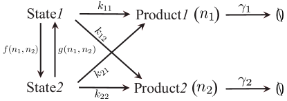
Figure 2: Schematics of a two-scale kinetic model with two kinds of products.

We assume similar scaling as considered in (16):

$$k_{ij}\sim\frac{1}{\epsilon},\quad f,g\sim\frac{1}{\epsilon^{\alpha}},\quad\alpha>0,\quad(i,j=1,2).$$

Define $x_{j}=n_{j}\epsilon$, $\tilde{k}_{ij}=k_{ij}\epsilon$ for $i,j=1,2$ and $\tilde{f}(x_{1},x_{2})=f(n_{1},n_{2})\epsilon^{\alpha}$, $\tilde{g}(x_{1},x_{2})=g(n_{1},n_{2})\epsilon^{\alpha}$. Performing the same approach as in Sec. II, we get the transition probability

$$P(n_{f},\tau|n_{i},0)\propto\int D\boldsymbol{x}D\boldsymbol{c}\exp\left(-\frac{1}{\epsilon}\int dtL_{1}(\boldsymbol{x},\dot{\boldsymbol{x}},\boldsymbol{c})-\frac{1}{\epsilon^{\alpha}}\int dtL_{2}(\boldsymbol{x},\boldsymbol{c})\right).$$

Here the Lagrangian

$$L_{1}(\boldsymbol{x},\dot{\boldsymbol{x}},\boldsymbol{c})=\mathop{\sup}_{\boldsymbol{p}}\{\boldsymbol{p}\cdot\dot{\boldsymbol{x}}-\tilde{H}_{1}(\boldsymbol{x},\boldsymbol{c},\boldsymbol{p})\},\quad L_{2}(\boldsymbol{x},\boldsymbol{c})=\mathop{\sup}_{\boldsymbol{\varphi}}\{-\tilde{H}_{2}(\boldsymbol{x},\boldsymbol{c},\boldsymbol{\varphi})\},$$

where $\boldsymbol{x}=(x_{1},x_{2})$, $\boldsymbol{c}=(c_{1},c_{2})$, $\boldsymbol{p}=(p_{1},p_{2})$, $\boldsymbol{\varphi}=(\varphi_{1},\varphi_{2})$ and

$$\tilde{H}_{1}(\boldsymbol{x},\boldsymbol{c},\boldsymbol{p}) = (\tilde{k}_{11}c_{1}+\tilde{k}_{21}c_{2})(e^{p_{1}}-1)+\gamma_{1}x_{1}[e^{-p_{1}}-1]+(\tilde{k}_{12}c_{1}+\tilde{k}_{22}c_{2})(e^{p_{2}}-1)+\gamma_{2}x_{2}(e^{-p_{2}}-1),$$

$$\tilde{H}_{2}(\boldsymbol{x},\boldsymbol{c},\boldsymbol{\varphi}) = c_{1}\tilde{g}(x)(e^{{\varphi}_{1}-{\varphi}_{2}}-1)+c_{2}\tilde{f}(x)(e^{{\varphi}_{2}-{\varphi}_{1}}-1).$$

All of the analysis performed for the two-state model can be applied here to obtain the LDTs for variable $\boldsymbol{x}=(x_{1},x_{2})$ with different $\alpha$.

One can also employ the WKB ansatz $P_{j}(x)\sim\exp(-\epsilon^{-1}\Phi_{j}(x))$ for the stationary distribution of the stochastic hybrid system (36), where $x=n\epsilon$ and $j$ is a state of DNA. In the asymptotics, one gets a static Hamilton-Jacobi equation for the quasi-potential $\Phi_{j}$ and it turns out $\Phi_{j}$ does not depend on the specific choice of $j$. However if not handled appropriately, the WKB approximation may lead to totally different forms of Hamiltonian LiLin as mentioned in the end of Section IV. This non-uniqueness is due to the lack of variational selection in LDT, which gives a unique Hamiltonian dual to the obtained Lagrangian in rate functional. And this Hamiltonian has the superiority that it is convex with respect to the momentum variable as the by-product of Legendre-Fenchel transform and LDT. This property is important for the nice behavior of numerical discretization.

In this paper, we assume the switching rates between different DNA states are in order $\epsilon^{-\alpha}$. It is not necessary and could be more general. As long as the switching rates between different DNA states are in $O(\lambda(\epsilon))$, and the cases $\lim_{\epsilon\to 0+}\epsilon\lambda(\epsilon)=\infty,~{}O(1)$ and $0$ are considered, we will get similar results. Especially, the readers may easily verify that if we assume $\lambda(\epsilon)=K\epsilon^{-1}$, then the two-scale LDT Lagrangian with $\epsilon$-scaling in front of $-\ln P$ has the form

$$L_{x}(x,\dot{x})=\mathop{\inf}_{\boldsymbol{c}}\left\{L_{1}(x,\dot{x},\boldsymbol{c})+KL_{2}(x,\boldsymbol{c})\right\},$$ (90)

and the LDT Lagrangian with $\lambda(\epsilon)$-scaling in front of $-\ln P$ has the form

$$L_{x}(x,\dot{x})=\mathop{\inf}_{\boldsymbol{c}}\left\{K^{-1}L_{1}(x,\dot{x},\boldsymbol{c})+L_{2}(x,\boldsymbol{c})\right\}.$$ (91)

When $K$ goes to $0,1$ or $\infty$, the appropriate choices of scaling recover the desired results shown in the paper.

In conclusion, we established the two-scale LDTs for a class of chemical reaction kinetics through the second-quantization path integral formulation. Although not rigorous, we showed that this formal approach is very effective and transparent to understand the two-scale LDTs associated with different reaction channels. This provides essential insights to rigorously prove the corresponding LDTs, which is our ongoing research. We discussed its implication on single-molecule Michaelis-Menten kinetics as well. The proposed framework and results also shed lights on the understanding of general multi-scale systems including diffusion processes. It will be interesting to investigate the application of two-scale LDTs to other systems.

References

References

• (1) Assaf M, Roberts E and Luthey-Schulten Z 2011 Determining the Stability of Genetic Switches: Explicitly Accounting for mRNA Noise Phys. Rev. Lett. 106 2048102.
• (2) Bender C M and Orszag S A 1999 Advanced Mathematical Methods for Scientists and Engineers: Asymptotic Methods and Perturbation Theory (New York: Springer) .
• (3) Bressloff P C and Faugeras O 2014 On the Hamiltonian structure of large deviations in stochastic hybrid systems arXiv:1410.2152v1.
• (4) Bressloff P C and Newby J M 2013 Metastability in a Stochastic Neural Network Modeled as a Velocity Jump Markov Process SIAM Appl. Dyn. Syst. 12 1394.
• (5) Bühler O 2006 A Brief Introduction to Classical, Statistical and Quantum Mechanics (Providence: American Mathematical Society).
• (6) Dembo A and Zeitouni O 1998 Large deviations techniques and applications, 2nd edition (New York: Springer- Verlag).
• (7) Doi M 1976 Second quantization representation for classical many-particle system J. Phys. A: Math. Gen. 9 1465.
• (8) Faggionato A, Gabrielli D and Crivellari M R 2010 Averaging and large deviation principles for fully-coupled piecewise deterministic Markov processes and applications to molecular motors Markov Process. Relat. Fields 16 497.
• (9) Freidlin M I and Wentzell A D 1998 Random perturbations of dynamical systems, 2nd edition (New York: Springer) .
• (10) Ge H, Qian H and Xie X S 2015 Stochastic phenotype transition of a single cell in an intermediate region of gene state switching Phys. Rev. Lett. 114 078101.
• (11) Heymann M and Vanden-Eijnden E 2008 The geometric minimum action method: A least action principle on the space of curves Comm. Pure Appl. Math. 61 1052.
• (12) Keener J and Sneyd J 1998 Mathematical Physiology (New York: Springer-Verlag).
• (13) Kemeny J G and Snell J L 1960 Finite Markov chains (New York, Berlin and Heidelberg: Springer-Verlag) .
• (14) Kou S C, Cherayil B J, Min W, English B P and Xie X S 2005 Single-molecule Michaelis-Menten Equations J. Phys. Chem. B 109 19068.
• (15) Li T and Lin F 2015 Large deviations for two-scale chemical kinetic processes arXiv:1504.03781.
• (16) Liptser R 1996 Large deviations for two scaled diffusions Prob. Theory Relat. Fields 106 71.
• (17) Lv C , Li X, Li F and Li T 2014 Constructing the energy landscape for genetic switching system driven by intrinsic noise PLoS ONE 9 e88167.
• (18) Lv C , Li X, Li F and Li T 2014 Energy landscape reveals that the budding yeast cell cycle is a robust and adaptive multi-stage process PLoS Comp. Biol. 9 e88167.
• (19) Michaelis L and Menten M L 1913 Die Kinetik der Invertinwerkung Biochem. Z. 49 333.
• (20) Newby J M 2012 Isolating intrinsic noise sources in a stochastic genetic switch Phys. Biol. 9 026002.
• (21) Newby J M 2014 Spontaneous Excitability in the Morris CLecar Model with Ion Channel Noise SIAM J. Appl. Dyn. Syst. 13 1756.
• (22) Newby J M and Bressloff P C 2010 Local synaptic signaling enhances the stochastic transport of motor-driven cargo in neurons Phys. Biol. 7 036004.
• (23) Newby J M and Chapman J 2014 Metastable behavior in Markov processes with internal states J. Math. Biol. 69 941.
• (24) Peliti L 1985 Path integral approach to birth-death processes on a lattice J. Phys. 46 1469.
• (25) Rockafellar R T and Wets R J B 1998 Variational Analysis (Berlin and HeidelbergSpringer) .
• (26) Shwartz A and Weiss A 1995 Large deivations for performance analysis: queues, communications and computing (London: Chapman and Hall).
• (27) Touchette H 2009 The large deviation approach to statistical mechanics Phys. Rep. 478 1.
• (28) Varadhan S R S 1984 Large deviations and applications (Philadelphia: SIAM) .
• (29) Veretennikov A Yu 2000 On large deviations for SDEs with small diffusion and averaging Stoch. Process. Appl. 89 69.
• (30) Veretennikov A Yu 1999 On large deviations in the averaging principle for SDE’s with a ”full dependence” Ann. Prob. 27 284.
• (31) Zhang B and Wolyness P G 2014 Stem cell differentiation as a many-body problem Proc. Natl. Acad. Sci. U.S.A. 111 10185.
• (32) Zhang K, Sasai M and Wang J 2013 Eddy current and coupled landscapes for nonadiabatic and nonequilibrium complex system dynamics Proc. Natl. Acad. Sci. U.S.A. 110 14930.
• (33) Zhou P and Li T 2015 Realization of Waddington’s metaphor: Potential landscape, quasi-potential, A-type integral and beyond arXiv:1511.02088 .