Scaling Analysis of Random Walks with Persistence Lengths: Application to Self-Avoiding Walks

Abstract

We develop an approach for performing scaling analysis of $N$-step Random Walks (RWs). The mean square end-to-end distance, $\langle\vec{R}_{N}^{2}\rangle$, is written in terms of inner persistence lengths (IPLs), which we define by the ensemble averages of dot products between the walker’s position and displacement vectors, at the $j$-th step. For RW models statistically invariant under orthogonal transformations, we analytically introduce a relation between $\langle\vec{R}_{N}^{2}\rangle$ and the persistence length, $\lambda_{N}$, which is defined as the mean end-to-end vector projection in the first step direction. For Self-Avoiding Walks (SAWs) on 2D and 3D lattices we introduce a series expansion for $\lambda_{N}$, and by Monte Carlo simulations we find that $\lambda_{\infty}$ is equal to a constant; the scaling corrections for $\lambda_{N}$ can be second and higher order corrections to scaling for $\langle\vec{R}_{N}^{2}\rangle$. Building SAWs with typically one hundred steps, we estimate the exponents $\nu_{0}$ and $\Delta_{1}$ from the IPL behavior as function of $j$. The obtained results are in excellent agreement with those in the literature. This shows that only an ensemble of paths with the same length is sufficient for determining the scaling behavior of $\langle\vec{R}_{N}^{2}\rangle$, being that the whole information needed is contained in the inner part of the paths.

year number number identifier

I INTRODUCTION

Random Walk (RW) models are ubiquitous in the literature with applications in several areas, such as Physics N_Stanley_2001 , Biology JRSI_Codling_2008 and Economy Book_IEC_1999 . The simplest case is the walker displacement in a sequence of independent random steps, namely ordinary RW Book_FSRW_2013 . One may also obtain random paths on a geometrical space with distinct displacement schemes, leading to other RW models. A fundamental importance of these models lies in the fact that many real phenomena can be mapped or directly represented by paths traversed by walkers in some geometrical space, e.g., a single-strand DNA JCP_Rechendorff_2009 and magnetic systems PRB_Heiko_1998 . An example is the Self-Avoiding Walk (SAW) defined by a walker forming a random path that never intersects itself; standard SAWs are performed on regular lattices, where the walker steps to nearest-neighbor sites and does not visit a site more than once Book_Madras_2012 .

Because of non-overlapping paths, the SAW model plays a central role in Polymer Physics Book_PP_2003 by capturing the excluded volume effect in a dilute solution under good solvent condition or at high temperatures PRB_Stanley_1987 . The SAW model is also well known in statistical physics context because of its equivalence with the $n$-vector model with $n\rightarrow 0$, as de Gennes first pointed out Book_DeGennes_1979 . From this equivalence, with arguments of renormalization and field theories, one expects the following series expansion for the mean square end-to-end distance JPA_Janse_2009 ; Belorec_1997 :

$$\langle\vec{R}_{N}^{2}\rangle_{N}=a_{0}N^{2\nu_{0}}(1+\frac{a_{1}}{N}+\frac{a_{2}}{N^{2}}+\cdots\frac{b_{1}}{N^{\Delta_{1}}}+\\ +\frac{b_{2}}{N^{\Delta_{1}+1}}+\cdots\frac{c_{1}}{N^{\Delta_{2}}}+\frac{c_{2}}{N^{\Delta_{2}+1}}+\cdots),$$ (1)

where $\nu_{0}$ is the leading exponent. The terms proportional to $N^{-i}$ with $i=1,2,\cdots$, are analytical corrections, and the terms proportional to $N^{-(j+\Delta_{i})}$ with non-integer exponents $\Delta_{i}<\Delta_{i+1}$ and $j=0,1,2\cdots$, are the non-analytical corrections to scaling. The leading and corrections to scaling exponents are universal. The indexed brackets $\langle.\rangle_{N}$ refers to the $N$-step RW ensemble average, and from now on, unless strictly necessary, we omit the index $N$. Numerical estimates of exponents $\nu_{0}$ and $\Delta_{1}$ are based on either exact counting techniques PRL_Fricke_2014 ; JSM_Schram_2011 , or in Monte Carlo (MC) simulation methods JSP_Madras_1988 ; JSP_HPS_2011 , through the sampling of $\langle\vec{R}_{N}^{2}\rangle$ PRL_Clisby_2010 ; JSP_Clisby_2010 .

Obtaining such estimates for $\nu_{0}$ and $\Delta_{1}$, especially for 3D SAW, is a challenge from several points of view. The exponential growth of the number of possible $N$-step paths $c_{N}\approx\mu^{N}N^{\gamma-1}$, where $\mu$ is the connectivity constant and $\gamma>1$, imposes a limit to exact counting. To the best of our knowledge, the maximum values obtained are $N=79$ Arx_Jensen_2013 and $N=36$ JSM_Schram_2011 for SAWs on 2D and 3D square lattices, respectively. Concerning Monte Carlo simulations, there exist an appeal to find $\nu_{0}$ and $\Delta_{1}$ using very long paths. Obtaining high quality Monte Carlo data for such path lengths is an extremely difficult task for the SAW model. The variable length algorithms suffer from attrition problems, namely barriers that prevent paths to grow, while the fixed length algorithms suffer from the decreasing of acceptance rate to generate a new non-self-intersecting path, according to the increase of the (fixed) path length NPB_Sokal_1996 .

Numerical drawbacks also take place when one studies other conformational quantities. An example is the persistence length, $\lambda_{N}$, defined as the mean end-to-end vector projection in a fixed direction along the first step Book_Cantor_1980 ; PNAS_Flory_1973 , as $N\rightarrow\infty$ Note1 . Defining the end-to-end vector as $\vec{R}_{N}=\sum_{j=1}^{N}\vec{u}_{j}$, where $\vec{u}_{j}$ is the walker displacement at the $j$-th step, the persistence length can be expressed by $\lambda_{N}=\langle\vec{R}_{N}\cdot\vec{u}_{1}\rangle/|\vec{u}_{1}|=\sum_{j=1}^{N}\langle\vec{u}_{1}\cdot\vec{u}_{j}\rangle/|\vec{u}_{1}|$. Numerical results of $\lambda_{N}$, for 2D-SAWs, are controversial in the literature, and for 3D, are scarce AIP_Hagai_1990 . For 2D-SAW, Grassberger PLA_Grassberger_1982 obtained the first estimate of $\lambda_{N}$ in the square lattice, by means of a power law $\lambda_{N}\sim N^{\theta}$, with $\theta=0.063(10)$. Since for $\theta\approx 0$, it is also well fitted by $\lambda_{N}\sim\ln(N)$, as suggested by Redner and Privmann JPA_Privman_1987 . They obtained both estimates by sampling the displacements projections along the first step direction, for all possible configurations of SAW paths with $N<24$. This weak divergence has been questioned recently by Eisenberg and Baram JPA_Eisenberg_2003 , because their MC estimates of $\langle\vec{u}_{1}\cdot\vec{u}_{j}\rangle$ show that $\lambda_{N}$ converges to a constant when $N\rightarrow\infty$. One could employ $\lambda_{N}$ in Monte Carlo Group and experimental characterization of certain polymers PNAS_Sitlani_2000 ; CP_Dogsa_2014 , despite there exist some limitations of $\lambda_{N}$ measures such as divergence and edge effects Group2 .

Refined results about the scaling behavior of the aforementioned conformational quantities to study universality are challenging, and have been the subject of discussion for many years JSP_Madras_1988 ; JPA_Janse_2009 . As usually one does not have exact results for the SAW model, there exists an appeal for simulations of large, sometimes very large, paths. Here, one proposes to answer two questions about a SAW: (i) What is the asymptotic limit of its persistence length? (ii) Is there some way to find out its scaling behavior employing relatively small chains? To answer these questions, we found an approach for performing scaling analysis of RWs, by focusing in the behavior of $\langle\vec{R}_{N}^{2}\rangle$.

The structure of the paper is as follows: In Sec. II we present the analytical results by defining the inner persistence length and their relation with $\langle\vec{R}_{N}^{2}\rangle$ and $\lambda_{N}$, for RW models statistically invariant under orthogonal transformations. In Sec. III we provide a series expansion for $\lambda_{N}$ and obtain the scaling behavior of 2D and 3D-SAW models with Monte Carlo simulations; we also obtain reliable estimates of the exponents $\nu_{0}$ and $\Delta_{1}$ and discuss the contribution of $\lambda_{N}$ to $\langle\vec{R}_{N}^{2}\rangle$ behavior. In Sec. IV we give concluding remarks.

II INNER PERSISTENCE LENGTH AND ANALYTICAL RESULTS

We define the inner persistence length (IPL) for an $N$-step RW, by the average dot product: $\mathcal{I}_{j}\equiv\langle\vec{R}_{j}\cdot\vec{u}_{j}\rangle$. To relate $\langle\vec{R}_{N}^{2}\rangle$ to $\mathcal{I}_{j}$, and $\mathcal{I}_{N}$ to $\lambda_{N}$, we write the square distance at the $j$-th step for an $N$-step RW as: $\vec{R}_{j}^{2}=\vec{R}_{j-1}^{2}+2\vec{R}_{j}\cdot\vec{u}_{j}-u_{j}^{2}$. Adding up $\vec{R}_{j}^{2}$, we have $\sum_{j=1}^{k}\vec{R}_{j}^{2}=\sum_{j=1}^{k}\vec{R}_{j-1}^{2}+\sum_{j=1}^{k}2\vec{R}_{j}\cdot\vec{u}_{j}-\sum_{j=1}^{k}|\vec{u}_{j}|^{2}$, where $\vec{R}_{0}=\vec{0}$ leads to $\sum_{j=1}^{k}\vec{R}_{j-1}^{2}=\sum_{j=1}^{k-1}\vec{R}_{j}^{2}$. Thus, considering $|\vec{u}_{j}|=1$, we write the average $\langle\vec{R}_{k}^{2}\rangle=2\sum_{j=1}^{k}\mathcal{I}_{j}-k$. In particular for $k=N$, the mean square end-to-end distance is

$$\langle\vec{R}_{N}^{2}\rangle=2\sum_{j=1}^{N}\mathcal{I}_{j}-N.$$ (2)

Now, consider a generic class of RWs, where ensembles of $N$-step walks obey the following invariance property: the probability distributions, of each step $\vec{u}_{i}$, $i=1,2,...,N$, which compose a path, is invariant under orthogonal transformations. With this, we exclude walks like the tourist model PRE_Lima_2001_1 , where the medium disorder Group3 breaks down such invariance symmetries. Particularly, one considers an ensemble of $N$-step RWs obeying the mentioned probabilistic symmetry, under a specific orthogonal transformation $T$ given by $\vec{u}_{i}\overset{T}{\rightarrow}\vec{u}_{N-i+1}^{\prime}$; the prime denotes the displacement vectors in the transformed reference frame, and $\vec{u}_{i}^{\prime}=-\vec{u}_{N-i+1}$, with $i=1,2,...N$. Notice that $\vec{u}_{i}^{\prime}\in\{\vec{u}_{1},\vec{u}_{2}...\vec{u}_{N}\}$, where $\{.\}$ represents the complete ensemble of paths. This symmetry operation can be achieved by a translation followed by inversion of all displacement vectors. In other words, one does invert each path and change the origin to the end of the walk. An immediate consequence for the complete ensemble of random paths is $\{\vec{u}_{i}\}=\{\vec{u}_{i}^{\prime}\}$, with $i=1,2,...N$, which leads to $\{\vec{R}_{N}\}=\{\vec{R}_{N}^{\prime}\}$. From the previous relations, it follows that $\{\vec{R}_{N}\cdot\vec{u}_{N}\}=\{\vec{R}_{N}\cdot\vec{u}_{1}\}$, so the configurational average $\langle\vec{R}_{N}\cdot\vec{u}_{N}\rangle=\langle\vec{R}_{N}\cdot\vec{u}_{1}\rangle$ holds. This average, for $N\rightarrow\infty$, is the persistence length $\lambda_{N}$. Therefore, the mean square end-to-end distance could be rewritten as

$$\langle\vec{R}_{N}^{2}\rangle=\langle\vec{R}_{N-1}^{2}\rangle+2\lambda_{N}-1,$$ (3)

and we have established a relation between $\langle\vec{R}_{N}^{2}\rangle$ and $\lambda_{N}$. We observed Eq. 3 numerically, prior to its proof, by exact calculations for $N\leq 24$. Some RW models that obey such a relation are the $N$-step ensemble of ordinary RW and SAW paths.

III NUMERICAL RESULTS FOR THE SAW MODEL

From now on, we numerically study $\mathcal{I}_{j}$ for SAWs using the non-reversed random walk (NRRW) algorithm to generate the ensemble of $N$-step non-overlapping paths. Because of the attrition problem, i.e., barriers or traps that prevent paths to achieve $N$ steps, the NRRW is inefficient to generate good statistics for long SAWs, since the probability decays as $p_{N}\propto\exp[-\gamma N]$, where $0<\gamma<1$ is the attrition constant. However, the generated data with this algorithm are surprisingly good enough to validate our approach, showing that we choose the right corrections to scaling terms in the expansion of IPLs.

Starting with $\langle\vec{R}_{N}^{2}\rangle$, we now analyze the persistence length. For the square lattice, $\nu_{0}=3/4$ JPA_Jensen_2004 and a common belief is that $\Delta_{1}=3/2$ JSP_Caracciolo_2005raey . With these exponents values, from Eq. 1, using only the first two leading exponents, we see that $\langle\vec{R}_{N}^{2}\rangle$ $\approx AN^{3/2}+BN^{1/2}$. The same reasoning leads to a similar result for cubic lattices, where $\nu_{0}\sim 0.587597(7)$ and $\Delta_{1}\sim 0.528(12)$ are widely accepted values PRL_Clisby_2010 . Both averages in Eq. 3, $\langle\vec{R}_{N}^{2}\rangle$ and $\langle\vec{R}_{N-1}^{2}\rangle$, are obtained considering the same $N$-step ensemble. In this sense, we follow our previous notation by omitting the bracket index. The difference $\langle\vec{R}_{N}^{2}\rangle-\langle\vec{R}_{N-1}^{2}\rangle$ seems to be the discrete derivative of square end-to-end distance, which is not true for the SAW model. One should evaluate the derivative considering SAW ensembles of $N$ and $(N-1)$-steps: $\langle\vec{R}_{N}^{2}\rangle_{N}-\langle\vec{R}_{N-1}^{2}\rangle_{N-1}$. According to Eq. 1, the leading term of $\langle\vec{R}_{N}^{2}\rangle_{N}$ derivative is $N^{2\nu_{0}-1}$ with the first two corrections proportional to $N^{2\nu_{0}-2}$ and $N^{2\nu_{0}-\Delta_{1}-1}$, respectively. From the persistence length plots in Fig. 1, $\lambda_{N}$ clearly does not diverge as the leading term of $\langle\vec{R}_{N}^{2}\rangle$ derivative, instead it seems to converge to a constant as $N$ goes to infinity Note2 . Thus, we introduce the following series expansion:

$$\lambda_{N}=\alpha_{0}+\alpha_{1}N^{-w_{1}}+\alpha_{2}N^{-w_{2}}+\cdots$$ (4)

where the exponents $w_{i}>0$, $i=1,2,3\cdots$, are linear combinations of $\nu_{0}$ with analytical and non-analytical corrections to scaling exponents. As for example, from the persistence length data fitting with Eq. 4 (see Fig. 1), we find that $w_{1}=2\nu_{0}-2$ and $w_{2}=2\nu_{0}-\Delta_{1}-1$ are the best choices. The $\alpha_{i}$ and $w_{i}$ values are shown in Tab. 1. An immediate consequence of such findings along with Eq. 3, is that $\lambda_{N}$ could contribute only with second and higher-order of analytic and non-analytic corrections for $\langle\vec{R}_{N}^{2}\rangle$. Our estimate of $\lambda_{N}$, for square lattices, is compatible with the one of Eisenberg and Baram JPA_Eisenberg_2003 . Through their estimate of the step-step correlation scaling: $\langle\vec{u}_{1}\cdot\vec{u}_{j}\rangle=\langle\xi_{1,j}\rangle_{N}\sim 0.6j^{-1.34(5)}$, and the definition $\lambda_{N}=\sum_{j=1}^{N}\langle\xi_{1,j}\rangle_{N}$, we obtained $\lambda_{N}\sim\alpha_{0}-1.7N^{-0.34(5)}$, with which we fitted the persistence length data, but leaving $\alpha_{1}$ free, as shown in the inset of Fig. 1(a).

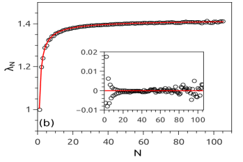
Figure 1: SAW persistence length for (a) square and (b) cubic lattices. In both lattices, $\lambda_{N}$ converges to a constant. The inset plot (a) shows $\lambda_{N}$ fitted by the function $\alpha_{0}+\alpha_{1}N^{-0.34}$ of Ref. JPA_Eisenberg_2003 , where $\lambda_{\infty}=2.664(3)$ is compatible with our estimate $\lambda_{\infty}=2.525(4)$ from Eq. 4. For the cubic lattice, $\lambda_{\infty}\sim\sqrt{2}$ is compatible with the one of Ref. AIP_Hagai_1990 . The inset plot (b) depicts the random pattern of the residual plot for $\lambda_{N}$ when fitted by Eq. 4.

Table 1: Coefficients and exponents for fitting, with Eq. 4, the $\lambda_{N}$ data obtained from simulations for 2D and 3D square lattices. The $w_{1}=0.34(5)$ value is an effective exponent, thus depending on the coefficients $\alpha_{i}$ and exponents $w_{i}$ of Eq. 4 JSP_Caracciolo_2005raey .

$d$	$\alpha_{0}$	$\alpha_{1}$	$\alpha_{2}$	$w_{1}$	$w_{2}$
$2$	$2.525(4)$	$-2.32(3)$	$0.81(3)$	$0.5$	$1$
$2$	$2.664(3)$	$-1.714(9)$	$-$	$0.34$	$-$
$3$	$1.422(1)$	$-0.39(6)$	$-0.022(5)$	$0.8248$	$0.34$

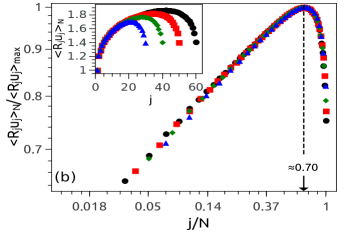
Figure 2: IPL data collapse in $\log$-$\log$ scale for (a) square and (b) cubic lattices with ($\color[rgb]{0,0,1}\blacktriangle\,N=30$), ($\color[rgb]{0,0.6,0}\blacklozenge\,N=40$), ($\color[rgb]{1,0,0}\blacksquare\,N=50$) and ($\bullet\,N=60$). The $\langle\vec{R}_{j}\cdot\vec{u}_{j}\rangle_{N}$ behaves as linear increasing function up to $\sim j_{max}$, with a slope $\approx(2\nu_{0}-1)$. In both lattices $j_{max}\propto N$, with constant of proportionality close to each other ($\sim 0.7$). For $j>j_{max}$ the scalar products contribute to residual terms of corrections to scaling of $\langle\vec{R}_{N}^{2}\rangle$.

Now, consider $\mathcal{I}_{j}$, for $1<j<N$. According to the collapsed $\log\times\log$ plots of Fig. 2, it is notable that $\mathcal{I}_{j}$ looks like a straight line up to near the point where it reaches its maximum value, at the $j_{max}$ step, with a positive slope $\approx$ $2\nu_{0}-1$. From Eqs. 1 and 2, and Fig. 2, assuming $\mathcal{I}_{j}$ scales as $j^{2\nu_{0}-1}$ is reasonable, at least for $j<j_{max}$. Such proportionality leads us to look for reliable estimates of $\nu_{0}$, and corrections to scaling exponents, for SAW ensembles with $N$ not too large. To accomplish this aim, diminishing the influence of the $N$-step ensemble on estimates of scaling exponents is necessary. In other words, it is necessary to find a cutoff step $j=j_{c}(N)$, at which $\mathcal{I}_{j}$ begins to be noticeably influenced by the $N$-step SAW ensemble. Surely, we can neglect steps above $j_{max}$. To seek the $j_{c}(N)$ step, we use the difference between the IPLs of two $N$-step ensembles, one that contains $N_{1}$, and the other $N_{2}$ steps,

$$\Delta R_{j}(N_{1},N_{2})=\langle\vec{R}_{j}\cdot\vec{u}_{j}\rangle_{N_{2}}-\langle\vec{R}_{j}\cdot\vec{u}_{j}\rangle_{N_{1}},$$ (5)

where $N_{2}>N_{1}$. According to Fig. 3(a), the IPL has approximately the same behavior for the two path lengths, up to the middle of the shortest path, $j_{c}(N_{1})\sim N_{1}/2$, for square lattices. Similarly, for cubic lattices, it has the same behavior, up to a third of the shortest path $j_{c}(N_{1})\sim N_{1}/3$ [see Fig. 3(b)]. Therefore, using $j\leq j_{c}(N)$, with $j_{c}(N)=N/2$ and $j_{c}(N)=N/3$ for 2D and 3D lattices, respectively, it is suitable to estimate the scaling exponents through $\mathcal{I}_{j}$.

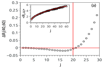
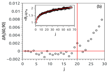
Figure 3: IPL differences ($\Delta R_{j}(N_{1},N_{2})$) for SAWs: (a) for square and (b) cubic lattices, with $N_{1}=40$ and $N_{2}=60$, and $N_{1}=60$ and $N_{2}=90$, respectively. According to $\Delta R_{j}(N_{1},N_{2})$ depicted here [see Eq.5], the $\mathcal{I}_{j}$ starts to be influenced for $j_{c}>N_{1}/2$ and $j_{c}>N_{1}/3$, for 2D and 3D square lattices, respectively. Inset plots show IPL non-weighted fit using Eq. 6, within a confidence interval of $95\%$. The square lattice data includes $N$ ranging from $90$ to $120$ with increment of 10. The fitting parameters obtained are $\varphi=0.4979(21)$ and $\beta_{1}=0.6630(50)$. The cubic lattice data includes $N$ ranging from $150$ to $195$ with increment of 15. The fitting parameters obtained are $\varphi=0.1752(14)$, $\Delta_{1}=0.522(52)$, and $\beta_{1}=0.7581(56)$.

Additional information to do scaling analysis with $\mathcal{I}_{j}$ comes from the expansion of $\langle\vec{R}_{N}^{2}\rangle$ in powers of $N$. We have found no evidence of the linear term in the expansion of $\langle\vec{R}_{N}^{2}\rangle$ on square or cubic lattices. The nonexistence of the linear term is also reported in Refs. JPA_Chan_2012 ; JPA_Lothar_1999 . From Eq. 2, the only way to disappear with the linear term in the expansion of $\langle\vec{R}_{N}^{2}\rangle$ is if the summation of $\mathcal{I}_{j}$ cancels it out. This finding, with Eq. 1, leads us to write

$$\mathcal{I}_{j}=\beta_{0}+\beta_{1}(j-\tau)^{\varphi}\left[1+\beta_{2}(j-\tau)^{-\Delta_{1}}+...\right],$$ (6)

for $j\leq j_{c}(N)$, where $\tau$ is a smoothing constant JPA_Clisby_2007 . We set $\beta_{0}=1/2$ just to cancel the linear term. Also, we did another ansatz: $\beta_{2}=-\left(2\nu_{0}-1\right)$ and $\tau=0.5$. This was inspired by results considering only the first non-analytical correction to scaling term, and leaving only the parameters $\beta_{1}$, $\beta_{2}$ and $\tau$ free, which lead us to find $\beta_{2}\approx-\left(2\nu_{0}-1\right)$ for the 3D case. Notice that, in general $\beta_{1}=\beta_{1}\left(N\right)$ and $\beta_{2}=\beta_{2}\left(N\right)$; however, for $N$ not too large, order of hundreds for 2D and 3D cases, these parameters converged to constants, for $j\leq j_{c}(N)$.

The IPL data, containing several $N$-step ensembles, fitted by Eq. 6 is depicted in the inset plots of Fig. 3. For both, the 2D and 3D square lattices, the leading and sub-leading exponents are in excellent agreement with the believed results. For the square lattice, we found $\nu_{0}=0.7489(21)$, and the non-analytical first exponent results in $\Delta_{1}=3/2$; because it does not appear in Eq. 6, showing that there exists a constant in the expansion of $\langle\vec{R}_{N}^{2}\rangle$. This is confirmed through the expansion of $\lambda_{N}$; the predicted results are $\varphi=0.5$ and $\Delta_{1}=3/2$. For cubic lattices we found $\nu_{0}=0.58757(140)$, and $\Delta_{1}=0.522(52)$, while the best predicted results are $\nu_{0}=0.587597(7)$ and $\Delta_{1}=0.528(12)$ PRL_Clisby_2010 . Using several $N$-step ensembles seeks to reduce the error on exponent estimates; however, they may carry some small biased errors. To check this, for 2D-SAW, we used $N=120$ steps obtaining $\nu_{0}=0.7500(63)$, and for 3D-SAW we used $N=198$ steps giving $\nu_{0}=0.58758(450)$ and $\Delta_{1}=0.52(17)$. However, the errors we get are not as small as those from literature for the 3D case PRL_Clisby_2010 . We can improve these results, by taking into account the advantage of the statistical invariance, and calculating the IPL starting from the end of the generated chains, thus doubling the sample. In fact, it is out of the scope of this paper to find high precision values for the exponents, but to validate and evaluate the benefits of our approach. Moreover, the whole potential of the method to do the scaling analysis of RWs has not been fully exploited. We expect that the corrections to scaling exponents are easily accessible from the study of the monotonically decreasing $\mathcal{I}_{j}$ terms of $\langle\vec{R}_{N}^{2}\rangle$, which will readily be tackled.

IV CONCLUDING REMARKS

In summary, we have proposed an approach to address the scaling of RW conformational quantities, where the mean square end-to-end distance is proportional to the summation of the inner persistence length, $\mathcal{I}_{j}=\langle\vec{R}_{j}\cdot\vec{u}_{j}\rangle$. For RW models, where paths obtained by orthogonal transformations occur with the same probability, we obtained a novel relation between the mean square end-to-end distance and persistence length. Despite the numerical limitations to do scaling analysis, we introduce a series for the persistence length $\lambda_{N}$ and show that it converges to a constant, $\alpha_{0}$, apart corrections to scaling terms. We also developed a method to calculate the scaling exponents from $\mathcal{I}_{j}$ with a path cutoff that diminishes the $N$-step ensemble influence. Thus, the method is efficient to obtain the scaling behavior of SAW.

We conclude that only an ensemble of paths with the same length is sufficient for performing scaling analysis, being that the whole information needed are contained in the inner part of the paths. The scaling method discussed in this paper can be important for studying universality, criticality, and conformational properties of systems mapped on RW models, such as polymers, biopolymers, and magnetic systems.

V ACKNOWLEDGMENTS

The authors thank T. J. Arruda, A. Caliri, J. C. Cressoni, G. M. Nakamura, and F. L. Ribeiro for their valuable comments. Also, the authors thank M. V. A. da Silva for exact enumeration SAW code and C. Traina for helpful discussions. C. R. F. Granzotti acknowledges CAPES for financial support. A. S. Martinez acknowledges CNPq (Grants No. 400162/2014-8 and No. 307948/2014-5) and NAP-FisMed for support. M. A. A. da Silva thanks Professor R. H. Swendsen for early fruitful discussions about scaling theory and SAWs and also, acknowledges FAPESP (Grants No. 11/06757-0 and No. 12/03823-5) for financial support.

References

- (1) H. E. Stanley, Nature 413, 373 (2001).
- (2) E. A. Codling, M. J. Plank, and S. Benhamou, J. R. Soc. Interface 5, 813 (2008).
- (3) R. N. Mantegna and H. E. Stanley, Introduction to econophysics: correlations and complexity in finance (Cambridge University Press, 1999).
- (4) J. Klafter and I. M. Sokolov, First Steps in Random Walks: From Tools to Applications (Oxford Scholarship Online, 2013).
- (5) K. Rechendorff, G. Witz, J. Adamcik, and G. Dietler, J. Chem. Phys. 131, 095103 (2009).
- (6) F. Iglói and H. Rieger, Phys. Rev. B 57, 11404 (1998).
- (7) N. Madras and G. Slade, The Self-Avoiding Walk, Modern Birkhäuser Classics (Springer, 2012).
- (8) M. Rubinstein and R. Colby, Polymer Physics (OUP Oxford, 2003).
- (9) A. Coniglio, Naeem Jan, I. Majid and Stanley, H. Eugene, Phys. Rev. B 35, 3617 (1987).
- (10) P. de Gennes, Scaling concepts in polymer physics (Cornell Univ. Pr., 1979).
- (11) E. J. J. van Rensburg, J. Phys. A-Math. Theor. 42, 323001 (2009).
- (12) P. Belohorec, Ph.D. thesis, The University of Guelph (1997).
- (13) N. Fricke and W. I. Janke, Phys. Rev. Lett. 113, 255701 (2014).
- (14) R. D. Schram, G. T. Barkema, and R. H. Bisseling, J. Stat. Mech-Theory. E 2011, P06019 (2011).
- (15) N. Madras and A. Sokal, J. Stat. Phys. 50, 109 (1988).
- (16) H.-P. Hsu and P. Grassberger, J. Stat. Phys. 144, 597 (2011).
- (17) N. Clisby, Phys. Rev. Lett. 104, 055702 (2010).
- (18) N. Clisby, J. Stat. Phys. 140, 349 (2010).
- (19) I. Jensen, arXiv:1309.6709, (2013).
- (20) A. D. Sokal, Nucl. Phys. B-Proc. Sup. 47, 172 (1996).
- (21) P. J. Flory, Proc. Nat. Acad. Sci. 70, 1819 (1973).
- (22) C. R. Cantor and P. R. Schimmel, Biophysical Chemistry: Part III (W. H. Freeman, 1980).
- (23) Notice that the persistence length for the wormlike chain model PRL_Ross_2013 ; MCR_Ullner_2006 (WLC) for semi-flexible polymers is defined as the characteristic decaying length of the correlation between unit tangent vectors at different points and of the chain, separated by a contour length . The correlation is given by , where the persistence length is mathematically equivalent to only for Porod_1949 ; MCR_Ullner_2002 .
- (24) B. C. Ross and P. A. Wiggins, Phys. Rev. E 87, 032707 (2013).
- (25) N. Makita, M. Ullner, and K. Yoshikawa, Macromolecules 39, 6200 (2006).
- (26) G. Porod, Monatsh. Chem Verw. Tl. 80, 251 (1949).
- (27) M. Ullner and C. E. Woodward, Macromolecules 35, 1437 (2002).
- (28) J. J. Weis and D. Levesque, Phys. Rev. Lett. 71, 2729 (1993); F.-H. Wang, Y.-Y. Wu, and Z.-J. Tan, Biopolymers 99, 370 (2013); L. Czapla, D. Swigon, and W. K. Olson, J. Mol. Biol. 382, 353 (2008).
- (29) M. Roychoudhury, A. Sitlani, J. Lapham, and D. Crothers, P Natl. Acad. Sci. USA 97, 13608 (2000).
- (30) I. Dogsa, M. Tomi, J. Orehek, E. Benigar, A. Jamnik, and D. Stopar, Carbohyd. Polym. 111, 492 (2014)
- (31) H.-P. Hsu, W. Paul, and K. Binder, Macromolecules 43, 3094 (2010); A. Huang, R. Adhikari, A. Bhattacharya, and K. Binder, Europhys. Lett. 105, 18002 (2014).
- (32) H. Meirovitch and H. Lim, J. Chem. Phys. 92, 5144 (1990).
- (33) P. Grassberger, Phys. Lett. A 89, 381 (1982).
- (34) S. Redner and V. Privman, J. Phys. A-Math. Gen. 20, L857 (1987).
- (35) E. Eisenberg and A. Baram, J. Phys. A-Math. Gen. 36, L121 (2003).
- (36) G. F. Lima, A. S. Martinez, and O. Kinouchi, Phys. Rev. Lett. 87, 010603 (2001).
- (37) C. R. F. Granzotti and A. S. Martinez, Eur. Phys. J. B. 87, 1 (2014); C. A. S. Terçariol and A. S. Martinez, Phys. Rev. E 72, 021103 (2005).
- (38) I. Jensen, J. Phys. A-Math. Gen. 37, 5503 (2004).
- (39) Notice that if the persistence length has a term proportional to or , it implies that the mean square end-to-end distance also has a or a logarithm correction term.
- (40) S. Caracciolo, A. J. Guttmann, I. Jensen, A. Pelissetto, A. N. Rogers, and A. D. Sokal, J. Stat. Phys. 120, 1037 (2005).
- (41) Y. ban Chan and A. Rechnitzer, J. Phys. A-Math. Theor. 45, 405004 (2012).
- (42) L. Schäfer, A. Ostendorf, and J. Hager, J. Phys. A-Math. Theor. 32, 7875 (1999).
- (43) N. Clisby, R. Liang, and G. Slade, J. Phys. A-Math. Theor. 40, 10973 (2007).