Compressive Sensing via
Low-Rank Gaussian Mixture Models

Abstract

We develop a new compressive sensing (CS) inversion algorithm by utilizing the Gaussian mixture model (GMM). While the compressive sensing is performed globally on the entire image as implemented in our lensless camera, a low-rank GMM is imposed on the local image patches. This low-rank GMM is derived via eigenvalue thresholding of the GMM trained on the projection of the measurement data, thus learned in situ. The GMM and the projection of the measurement data are updated iteratively during the reconstruction. Our GMM algorithm degrades to the piecewise linear estimator (PLE) if each patch is represented by a single Gaussian model. Inspired by this, a low-rank PLE algorithm is also developed for CS inversion, constituting an additional contribution of this paper. Extensive results on both simulation data and real data captured by the lensless camera demonstrate the efficacy of the proposed algorithm. Furthermore, we compare the CS reconstruction results using our algorithm with the JPEG compression. Simulation results demonstrate that when limited bandwidth is available (a small number of measurements), our algorithm can achieve comparable results as JPEG.

I Introduction

Compressive sensing [1, 2, 3] (CS) has led to real applications, including the single-pixel camera [4], the lensless camera [5, 6], video compressive sensing [7, 8, 9, 10, 11], depth compressive sensing [8, 12], hyperspectral compressive imaging [13, 14, 15], polarization compressive sensing [16], terahertz imaging [17], and millimeter wave imaging [18]. In this paper, we focus on the two-dimensional (2D) image case, though similar technique can be used for videos [19] and other bandwidths. Specifically, we develop our algorithm under the lensless compressive imaging architecture [5, 20], which has provided excellent reconstruction images from the compressive measurements using simple and off-the-shelf hardware [20].

Diverse algorithms [21, 22, 23, 24, 25, 26] have been developed for compressive sensing recovery, which plays a pivot role in CS, to reconstruct the desired signal from compressive measurements. Sparsity, the key ingredient of CS, has been investigated extensively in these algorithms. The wavelet transformation [27, 28, 29, 21] is generally used since it provides the sparse representation of an image with fast transformations (thus very efficient). A parallel research is using the total variation (TV) for CS recovery [23, 30], which provides good results for piecewise smooth signals. The aforementioned algorithms do not increase the unknown parameters significantly during the reconstruction, as usually the wavelet coefficients will have similar (or the same) number of the image pixels. Recently, researchers have found that by exploiting the sparsity of local patches [31, 32], better results can be achieved. In summary, CS recovery algorithms fall into the following three categories: 1) global basis based algorithm, e.g., using the wavelet transformation, 2) TV based algorithm, and 3) local basis based algorithm, i.e., DCT or dictionary learning or denoising based algorithms. State-of-the-art CS inversion results have been obtained in [33, 34], which generally lie within the third category. In this paper, we propose an alternative inversion algorithm that exploits the low-rank property of image patches.

Generally, the CS recovery is an iterative process in which two steps are performed at each iteration [34]: $i)$ projecting the measurements to the image level, which can be done by the majorization-minimization (MM) approach [22, 35], or the Euclidean projection [36], or the alternating direction method of multipliers (ADMM) [37], $ii)$ denoising this projected image and updating the recovery of the desired image. These two steps are performed iteratively until some criterion is satisfied. A general framework is developed in [34] under the approximate message passing (AMP) framework, in which diverse denoising algorithms [38] can be plugged in. One key difference of the denoising based CS inversion algorithms compared with the wavelet based CS inversion algorithms is that the former exploits the local sparsity based on (overlapping) patches, as state-of-the-art denoising algorithm is using sparse representation of local patches, e.g., [39]. The number of coefficients for the patches (under some basis or dictionary) is usually larger than the image pixel number (because the overlapping patches are used).

I-A Contributions

The proposed algorithm in this paper also lies in the third category mentioned earlier, which is based on the local basis (for image patches). Specific contributions of this work can be summarized as below:

• We investigate the low-rank property of image patches under the Gaussian mixture model (GMM) framework. Different from the low-rank model investigated in [33], which requires patch clustering (block matching) as an additional step, in our algorithm, each patch is modeled by a GMM with different weights corresponding to different Gaussian components, which can be seen as a soft clustering approach based on these weights. Furthermore, these weights are updated in each iteration.

• We develop an general framework using ADMM to explore the sparsity (and low-rank property) of patches in order to recover the desired signal.

• If each patch is modeled by a single Gaussian component, our GMM degrades to the piecewise linear estimator (PLE) [40, 41]. Therefore, a low-rank PLE algorithm is also proposed for CS recovery.

• We conduct experiments using our proposed algorithm and other leading algorithms on the real data captured by our lensless camera. This verifies real applications of each algorithm.

I-B Organization of This Paper

We start with the derivation of an ADMM formulation for CS recovery to investigate the sparsity of local overlapping patches in Section II. The proposed low-rank GMM algorithm is developed in Section III and the joint reconstruction algorithm is summarized in Section IV. Extensive results on both simulation and real data are reported in Sections V-VI. Section VII concludes the paper.

II CS Inversion via Exploiting Sparsity of Patches

Under the CS framework, the problem we are solving can be formulated as:

$$\min \frac{1}{2}\|\boldsymbol{y}-{\bf A}\boldsymbol{x}\|^{2}_{2}+\lambda\|\boldsymbol{z}\|_{1},$$ (1)

s.t. $$\boldsymbol{x}={\bf B}\boldsymbol{z},$$ (2)

where ${\bf A}\in{\mathbb{R}}^{M\times N}$ is the sensing matrix, $\boldsymbol{x}\in{\mathbb{R}}^{N}$ is the desired signal, $\boldsymbol{z}$ is the coefficients which are sparse under the basis ${\bf B}$. From $\boldsymbol{z}$, we can recover $\boldsymbol{x}$ easily via ${\bf B}$, which can be known a priori, (e.g., a wavelet or DCT basis) or learned based on $\boldsymbol{x}$ during the reconstruction.

Considering the image case investigated here, let $\boldsymbol{x}$ denote the vectorized image and the sparse representation, $\boldsymbol{z}$, is now modeled on image patches. Therefore, (2) can be reformulated as:

$${\bf R}\boldsymbol{x}={\bf B}\boldsymbol{z},$$ (3)

where $\bf{R}$ denotes the patch extraction and vectorization operation and considering each patch, we have

$${\bf R}_{i}\boldsymbol{x}={\bf B}\boldsymbol{z}_{i}$$ (4)

with $i$ indexes the patches.

The problem can be reformulated as:

$$\min \frac{1}{2}\|\boldsymbol{y}-{\bf A}\boldsymbol{x}\|^{2}_{2}+\lambda\|\boldsymbol{z}\|_{1},$$ (5)

s.t. $${\bf R}_{i}\boldsymbol{x}={\bf B}\boldsymbol{z}_{i}.$$ (6)

Note this ${\bf B}$ is shared for all patches for current discussion, and in the following analysis, similar patches can be grouped together [33] and each group can have its own ${\bf B}$.

Next, we develop an ADMM [37] formulation of (5) to solve the problem, which will also be used in our GMM formulation in Section IV. Introducing Lagrange multipliers ${\boldsymbol{\rho}}$ and parameter $\eta$ in (5) results in the objective function

$$L(\boldsymbol{x},\boldsymbol{z},\lambda,\rho) =\frac{1}{2}\|\boldsymbol{y}-{\bf A}\boldsymbol{x}\|^{2}_{2}+\lambda\|\boldsymbol{z}\|_{1}+{\boldsymbol{\rho}}^{\top}\sum_{i}({\bf R}_{i}\boldsymbol{x}-{\bf B}\boldsymbol{z}_{i})$$

$$\quad+\frac{\eta}{2}\sum_{i}\|{\bf R}_{i}\boldsymbol{x}-{\bf B}\boldsymbol{z}_{i}\|_{2}^{2}$$ (7)

Define ${\boldsymbol{u}}=(1/\eta){\boldsymbol{\rho}}$,

$$L(\boldsymbol{x},\boldsymbol{z},{\boldsymbol{u}},\lambda) = \frac{1}{2}\|\boldsymbol{y}-{\bf A}\boldsymbol{x}\|^{2}_{2}+\lambda\|\boldsymbol{z}\|_{1}$$ (8)

$$+\frac{\eta}{2}\sum_{i}\|{\bf R}_{i}\boldsymbol{x}-{\bf B}\boldsymbol{z}_{i}+{\boldsymbol{u}}\|_{2}^{2}+{\rm const}.$$

The ADMM cyclically solves the following 3 sub-problems:

$$\boldsymbol{x}^{t+1} :=\arg\min_{\boldsymbol{x}}(\frac{1}{2}\|\boldsymbol{y}-{\bf A}\boldsymbol{x}\|^{2}_{2}+\frac{\eta}{2}\sum_{i}\|{\bf R}_{i}\boldsymbol{x}-{\bf B}\boldsymbol{z}^{t}_{i}+{\boldsymbol{u}}^{t}\|_{2}^{2})$$ (9)

$$\boldsymbol{z}^{t+1} :=\arg\min_{\boldsymbol{z}}(\lambda\|\boldsymbol{z}\|_{1}+\frac{\eta}{2}\sum_{i}\|{\bf R}_{i}\boldsymbol{x}^{t+1}-{\bf B}\boldsymbol{z}_{i}+{\boldsymbol{u}}^{t}\|_{2}^{2})$$ (10)

$${\boldsymbol{u}}^{t+1} :={\boldsymbol{u}}^{t}+\sum_{i}({\bf R}_{i}\boldsymbol{x}^{t+1}-{\bf B}\boldsymbol{z}_{i}^{t+1})$$ (11)

where $t$ denotes the iteration index.

Equation (9) is a quadratic optimization problem and can be simplified to

$$({\bf A}^{\top}{\bf A}+\eta\sum_{i}{\bf R}_{i}^{\top}{\bf R}_{i}){\boldsymbol{x}}={\bf A}^{\top}\boldsymbol{y}+\eta\sum_{i}({\bf R}_{i}^{\top}{\bf B}\boldsymbol{z}_{i}-{\bf R}_{i}^{\top}{\boldsymbol{u}}^{t}),$$ (12)

which admits the closed-form solution,

$${\boldsymbol{x}}=({\bf A}^{\top}{\bf A}+\eta\sum_{i}{\bf R}_{i}^{\top}{\bf R}_{i})^{-1}[{\bf A}^{\top}\boldsymbol{y}+\eta\sum_{i}({\bf R}_{i}^{\top}{\bf B}\boldsymbol{z}_{i}-{\bf R}_{i}^{\top}{\boldsymbol{u}}^{t})].$$ (13)

However, the dimension of $({\bf A}^{\top}{\bf A}+\eta\sum_{i}{\bf R}_{i}^{\top}{\bf R}_{i})$ is large (the pixels of the desired image), requiring a high computational workload. Alternatively, since $({\bf A}^{\top}{\bf A}+\eta\sum_{i}{\bf R}_{i}^{\top}{\bf R}_{i})$ is invertible, the matrix inversion formula can be used to reduce the computational workload. As ${\bf R}_{i}$ is used to extract $i$-th patch from an image, $\sum_{i}{\bf R}_{i}^{\top}{\bf R}_{i}$ is a diagonal matrix

$$\tilde{\bf R}\stackrel{{\scriptstyle\rm def}}{{=}}\sum_{i}{\bf R}_{i}^{\top}{\bf R}_{i}={\rm diag}(r_{1},\dots,r_{N}).$$ (14)

Each of the diagonal entries corresponds to an image pixel location and its value is the number of overlapping patches that cover that pixel. Therefore, $\tilde{\bf R}^{-1}={\rm diag}(r_{1}^{-1},\dots,r_{N}^{-1})$ and

$$({\bf A}^{\top}{\bf A}+\eta\tilde{\bf R})^{-1}=\eta^{-1}\tilde{\bf R}^{-1}$$

$$-\eta^{-1}\tilde{\bf R}^{-1}{\bf A}^{\top}({\bf I}+{\bf A}\eta^{-1}\tilde{\bf R}^{-1}{\bf A}^{\top})^{-1}{\bf A}\eta^{-1}\tilde{\bf R}^{-1}.$$ (15)

However, this is not necessarily easy to calculate though $\tilde{\bf R}$ can be pre-computed. ${\bf A}\tilde{\bf R}^{-1}{\bf A}^{\top}$ needs to be saved for computation. Alternatively, (13) can be solved by the conjugate gradient algorithm [42].

To mitigate this problem, we apply the ADMM again on (5) and introduce another auxiliary variable $\boldsymbol{w}$, leading to the following optimization problem:

$$\min ~{}~{}\frac{1}{2}\|\boldsymbol{y}-{\bf A}\boldsymbol{x}\|^{2}_{2}+\lambda\|\boldsymbol{z}\|_{1}+\frac{\eta}{2}\sum_{i}\|{\bf R}_{i}\boldsymbol{w}-{\bf B}\boldsymbol{z}_{i}\|_{2}^{2},$$ (16)

s.t. $$~{}~{}\boldsymbol{x}=\boldsymbol{w}.$$ (17)

Following this,

$$(\boldsymbol{x},\boldsymbol{w},\boldsymbol{z},\boldsymbol{\alpha}) =\underset{\boldsymbol{x},\boldsymbol{w},\boldsymbol{z},\boldsymbol{\alpha}}{\arg\!\min}\frac{1}{2}\|\boldsymbol{y}-{\bf A}\boldsymbol{x}\|^{2}_{2}+\frac{\eta}{2}\sum_{i}\|{\bf R}_{i}\boldsymbol{w}-{\bf B}\boldsymbol{z}_{i}\|_{2}^{2}$$

$$+\lambda\|\boldsymbol{z}\|_{1}+\boldsymbol{\alpha}^{\top}(\boldsymbol{x}-\boldsymbol{w})+\frac{\beta}{2}\|\boldsymbol{x}-\boldsymbol{w}\|_{2}^{2}$$ (18)

which can be simplified to (by setting $\boldsymbol{v}=\boldsymbol{\alpha}/\beta$):

$$(\boldsymbol{x},\boldsymbol{w},\boldsymbol{z},\boldsymbol{v}) =\underset{\boldsymbol{x},\boldsymbol{w},\boldsymbol{z},\boldsymbol{v}}{\arg\!\min}\frac{1}{2}\|\boldsymbol{y}-{\bf A}\boldsymbol{x}\|^{2}_{2}+\frac{\eta}{2}\sum_{i}\|{\bf R}_{i}\boldsymbol{w}-{\bf B}\boldsymbol{z}_{i}\|_{2}^{2}$$

$$~{}~{}+\lambda\|\boldsymbol{z}\|_{1}+\frac{\beta}{2}\|\boldsymbol{x}-\boldsymbol{w}+\boldsymbol{v}\|_{2}^{2}+{\rm const}$$ (19)

The optimization of (II) consists of the following iterations:

$$\boldsymbol{x}^{t+1} :=\arg\min_{\boldsymbol{x}}\frac{1}{2}\|\boldsymbol{y}-{\bf A}\boldsymbol{x}\|^{2}_{2}+\frac{\beta}{2}\|\boldsymbol{x}-\boldsymbol{w}^{k}+\boldsymbol{v}^{t}\|_{2}^{2},$$ (20)

$$\boldsymbol{w}^{t+1} :=\arg\min_{\boldsymbol{w}}\frac{\eta}{2}\sum_{i}\|{\bf R}_{i}\boldsymbol{w}-{\bf B}\boldsymbol{z}^{t}_{i}\|_{2}^{2}$$

$$\qquad\qquad\qquad+\frac{\beta}{2}\|\boldsymbol{x}^{t+1}-\boldsymbol{w}+\boldsymbol{v}^{t}\|_{2}^{2},$$ (21)

$$\boldsymbol{z}^{t+1} :=\arg\min_{\boldsymbol{z}}\lambda\|\boldsymbol{z}\|_{1}+\eta\sum_{i}\|{\bf R}_{i}\boldsymbol{w}^{t+1}-{\bf B}\boldsymbol{z}_{i}\|_{2}^{2},$$ (22)

$$\boldsymbol{v}^{t+1} :=\boldsymbol{\boldsymbol{v}}^{t}+(\boldsymbol{x}^{t+1}-\boldsymbol{w}^{t+1}).$$ (23)

For fixed {$\boldsymbol{w}^{t},\boldsymbol{v}^{t}$}, $\boldsymbol{x}^{t+1}$ admits the following closed-form solution:

$$\boldsymbol{x}^{t+1} =({\bf A}^{\top}{\bf A}+\beta{\bf I})^{-1}[{\bf A}^{\top}\boldsymbol{y}+\beta(\boldsymbol{w}^{t}-\boldsymbol{v}^{t})],$$ (24)

which can be simplified to

$$\boldsymbol{x}^{t+1} =(\beta^{-1}{{\bf I}}-\beta^{-1}{\bf A}^{\top}({\bf I}+{\bf A}\beta^{-1}{\bf A}^{\top})^{-1}{\bf A}\beta^{-1})$$

$$\times[{\bf A}^{\top}\boldsymbol{y}+\beta(\boldsymbol{w}^{t}-\boldsymbol{v}^{t})],$$ (25)

For the case considered in our work (as implemented in the lensless camera [5]), ${\bf A}$ is the permuted Hadamard matrix and thus ${\bf A}{\bf A}^{\top}$ is an identity matrix:

$$\boldsymbol{x}^{t+1} =\left(\beta^{-1}{{\bf I}}-\frac{{\bf A}^{\top}{\bf A}}{(\beta+1)\beta}\right)[{\bf A}^{\top}\boldsymbol{y}+\beta(\boldsymbol{w}^{t}-\boldsymbol{v}^{t})]$$

$$=\frac{{\bf A}^{\top}\boldsymbol{y}}{\beta+1}+(\boldsymbol{w}^{t}-\boldsymbol{v}^{t})-\frac{{\bf A}^{\top}{\bf A}(\boldsymbol{w}^{t}-\boldsymbol{v}^{t})}{\beta+1}$$

$$=(\boldsymbol{w}^{t}-\boldsymbol{v}^{t})+\frac{{\bf A}^{\top}(\boldsymbol{y}-{\bf A}(\boldsymbol{w}^{t}-\boldsymbol{v}^{t}))}{\beta+1}.$$ (26)

Similarly, for fixed {$\boldsymbol{x}^{t+1},\boldsymbol{v}^{t},\boldsymbol{z}^{t}$}, $\boldsymbol{w}^{t+1}$ admits the following closed-form solution:

$$\boldsymbol{w}^{t+1} =\left(\eta\sum_{i}{\bf R}_{i}^{\top}{\bf R}_{i}+\beta{\bf I}\right)^{-1}$$

$$\quad\times\left[\beta(\boldsymbol{x}^{t+1}+\boldsymbol{v}^{t})+\eta\sum_{i}{\bf R}^{\top}_{i}{\bf B}\boldsymbol{z}_{i}^{t}\right]$$ (27)

Recall that $\sum_{i}{\bf R}_{i}^{\top}{\bf R}_{i}$ is a diagonal matrix $\tilde{\bf R}\stackrel{{\scriptstyle\rm def}}{{=}}{\rm diag}(r_{1},\dots,r_{N})$, thus $\boldsymbol{w}$ can be computed element wise via

$$w_{n}^{t+1} =\frac{\left[\beta(\boldsymbol{x}^{t+1}+\boldsymbol{v}^{t})+\eta\sum_{i}{\bf R}^{\top}_{i}{\bf B}\boldsymbol{z}_{i}^{t}\right]_{n}}{\eta r_{n}+\beta}$$ (28)

where $[\cdot]_{n}$ denotes the $n$-th entry of the vector inside $[~{}]$.

Similar to (10), (22) can be considered as a dictionary learning model, where ${\bf B}$ is the dictionary. If the orthonormal transformation is used (e.g., the DCT), $\boldsymbol{z}$ can be solved by the shrinkage thresholding operation [22, 27].

Since the key of this algorithm is to investigate the sparsity of the local overlapping patches, we term this framework as SLOPE (Shrinkage of Local Overlapping Patches Estimator), where the ‘local’ stands for the local basis rather than the global basis such as wavelet. The ADMM-SLOPE is summarized in Algorithm 1.

While good results have been obtained using similar approaches [31, 33] as in Algorithm 1, in the next section, we develop a low-rank GMM framework imposed on the patches and a full formulation of the proposed algorithm is presented in Section IV.

Algorithm 1 ADMM-SLOPE

0:  Measurements ${\boldsymbol{y}}$, sensing matrix ${\bf A}$, {$\beta$, $\eta$, $\lambda$}.

1:  Initial $\boldsymbol{x},\boldsymbol{w},\boldsymbol{v}$ to all 0.

2:  for $t=1$ to Max-Iter  do

3:     Update $\boldsymbol{x}$ by Eq. (II).

4:     Update $\boldsymbol{w}$ by Eq. (II).

5:     Update $\boldsymbol{z}$ by shrinkage operator.

6:     Update $\boldsymbol{v}$ by Eq. (23).

7:  end for

III The Gaussian Mixture Model

The Gaussian mixture model (GMM) has been re-recognized as an advanced dictionary learning approach and has achieved excellent results in image processing [40, 41] and video compressive sensing [43, 19]. Recall the image patches ${\bf X}\in{\mathbb{R}}^{P\times N_{p}}$ extracted from the 2D image, where the patch size is $\sqrt{P}\times\sqrt{P}$ and there are in total $N_{p}$ patches. For $i$-th patch $\boldsymbol{x}_{i}$, it is modeled by a GMM with $K$ Gaussians [44]:

$$\boldsymbol{x}_{i}\sim\sum_{k=1}^{K}\pi_{k}{\cal N}(\boldsymbol{\mu}_{k},\boldsymbol{\Sigma}_{k})$$ (29)

where $\{\boldsymbol{\mu}_{k},\boldsymbol{\Sigma}_{k}\}_{k=1}^{K}$ represent the mean and covariance matrix of $k$-the Gaussian, and $\{\pi_{k}\}_{k=1}^{K}$ denotes the weights of these Gaussian component.

In this paper, we further impose the GMM is low-rank and now the model in (2) becomes (29) and the problem to be solved becomes

$$\min \frac{1}{2}\|\boldsymbol{y}-{\bf A}\boldsymbol{x}\|^{2}_{2}$$ (30)

s.t. $$\boldsymbol{x}_{i}\sim\sum_{k=1}^{K}\pi_{k}{\cal N}(\tilde{\boldsymbol{\mu}}_{k},\tilde{\boldsymbol{\Sigma}}_{k})$$ (31)

where $\boldsymbol{x}_{i}$ denotes $i$-th patch from $\boldsymbol{x}$, which is an vectorized image. $\{\tilde{\boldsymbol{\mu}}_{k},\tilde{\boldsymbol{\Sigma}}_{k}\}_{k=1}^{K}$ symbolize the low-rank GMM.

The following problem is to estimate this low-rank GMM. Recalling Section I, we review that the CS recovery is an iterative two-step procedure. In each iteration, one can get an estimate from the projection of the measurements (details discussed in Section IV). We hereby learn a (full rank) GMM from this estimate and then proposing the eigenvalue thresholding approach to derive the low-rank GMM based on this full rank GMM.

III-A Low-Rank GMM

In the following, we provide a motivation for the next step in the algorithm. The random vector $\boldsymbol{x}_{i}$ in (29) (modeled as a GMM) can be written as, dropping the subscript $i$ for simplicity,

$$\boldsymbol{x}=\sum_{k=1}^{K}\pi_{k}{\boldsymbol{g}}_{k},$$ (32)

where each ${\boldsymbol{g}}_{k}$ is a random vector of multivariate normal distribution, given by

$${\boldsymbol{g}}_{k}\sim{\cal N}(\boldsymbol{\mu}_{k},\boldsymbol{\Sigma}_{k}).$$ (33)

The random vector ${\boldsymbol{g}}_{k}$ can be decomposed into independent random variables of normal distribution [45, 43] as follows

$${\boldsymbol{g}}_{k}={{\bf F}}_{k}{\boldsymbol{q}}_{k}+\boldsymbol{\mu}_{k},$$ (34)

where ${{\bf F}}_{k}\in{\mathbb{R}}^{P\times\gamma_{k}},{\boldsymbol{q}}_{k}\in{\mathbb{R}}^{\gamma_{k}}$, $\gamma_{k}$ is the rank of $\boldsymbol{\Sigma}_{k}$, and ${\boldsymbol{q}}_{k}$ is a vector whose $\gamma_{k}$ components are independent random variables.

In order to reduce noise, we use a model in which ${\boldsymbol{g}}_{k}$ has a small number of independent random components, i.e., we require $\gamma_{k}$ to be small. This is equivalent to requiring $\boldsymbol{\Sigma}_{k}$ have a reduced rank. More specifically, introducing the parameter $\tau_{k}$, we solve the following minimization problem [46]:

$$\tilde{\boldsymbol{\Sigma}}_{k}=\arg\min_{{\boldsymbol{\Gamma}}}\{{\frac{1}{2}\|{\boldsymbol{\Gamma}}-\boldsymbol{\Sigma}_{k}||^{2}_{F}}+\tau_{k}\|{\boldsymbol{\Gamma}}\|_{*}\},\quad\forall k=1,\cdots,K.$$ (35)

where $\|\cdot\|_{F}$ is the Frobenious norm, and $\|\cdot\|_{*}$ is the nuclear norm (sum of the singular values). It is shown in [46] that the solution to (35) can be readily obtained by a shrinkage on the singular values (which are similar to the eigenvalues) of $\boldsymbol{\Sigma}_{k}$. Specifically, consider

$$\boldsymbol{\Sigma}_{k} = {{\bf U}}_{k}\Lambda_{k}{{\bf U}}_{k}^{\top},$$ (36)

$$\Lambda_{k} = [\lambda_{1},\dots,\lambda_{P}].$$ (37)

We impose that $\gamma_{k}<P$ via

$$\tilde{\Lambda}_{k} = [\tilde{\lambda}_{1},\dots,\tilde{\lambda}_{r_{k}},{\bf 0}],$$ (38)

$$\tilde{\lambda}_{i} = \max(\lambda_{i}-\lambda_{\gamma_{k}+1},0),\quad\forall i=1,\dots,P.$$ (39)

And we term this as the eigenvalue thresholding (EVT). Following this, $\tilde{\boldsymbol{\Sigma}}_{k}$ is obtained by

$$\tilde{\boldsymbol{\Sigma}}_{k}={{\bf U}}_{k}\tilde{\Lambda}_{k}{{\bf U}}_{k}^{\top}.$$ (40)

We further define

$$\tilde{\boldsymbol{\mu}}_{k}=\boldsymbol{\mu}_{k},\quad\forall k=1,\cdots,K.$$ (41)

Next, we define a new random vector

$$\tilde{\boldsymbol{x}}_{i}\sim\sum_{k=1}^{K}{\pi}_{k}{\cal N}(\tilde{\boldsymbol{\mu}}_{k},\tilde{\boldsymbol{\Sigma}}_{k}),$$ (42)

which is modeled by a low-rank GMM, parameterized by $\{{\pi}_{k},\tilde{\boldsymbol{\mu}}_{k},\tilde{\boldsymbol{\Sigma}}_{k}\}_{k=1}^{K}$.

III-B Update Estimate via the Low-Rank GMM

Given an estimated image ${\hat{\boldsymbol{x}}}$, the GMM in (29) can be learned via the Expectation-Maximization (EM) algorithm [44, 43] based on overlapping patches. Then for each Gaussian component, we adopt the EVT to the covariance matrix to obtain the low-rank GMM $\{\tilde{\boldsymbol{\mu}}_{k},\tilde{\boldsymbol{\Sigma}}_{k}\}_{k=1}^{K}$. Following this, the estimated image $\hat{\boldsymbol{x}}$ or patches $\boldsymbol{x}_{i}$ can be updated via this low-rank GMM, to $\hat{\tilde{\boldsymbol{x}}}$ or ${\tilde{\boldsymbol{x}}}_{i}$. Dropping the subscript $i$, given ${\hat{\boldsymbol{x}}}$, the conditional distribution for $\hat{\tilde{\boldsymbol{x}}}$ maybe evaluated as

$$p(\hat{\tilde{\boldsymbol{x}}}|{\hat{\boldsymbol{x}}}) = \frac{p(\hat{\tilde{\boldsymbol{x}}})p(\hat{\boldsymbol{x}}|{\hat{\tilde{\boldsymbol{x}}}})}{\int p(\hat{\tilde{\boldsymbol{x}}})p(\hat{\boldsymbol{x}}|{\hat{\tilde{\boldsymbol{x}}}})d{\hat{\tilde{\boldsymbol{x}}}}}$$ (43)

Since ${\hat{\tilde{\boldsymbol{x}}}}$ is a low-rank version of $\hat{\boldsymbol{x}}$, we assume:

$$\hat{\boldsymbol{x}} = \hat{\tilde{\boldsymbol{x}}}+\boldsymbol{n},$$ (44)

where $\boldsymbol{n}\sim{\cal N}(0,{{\bf E}})$ is modeled as an additive Gaussian noise, thus

$$p(\hat{\boldsymbol{x}}|{\hat{\tilde{\boldsymbol{x}}}}) \sim {\cal N}({\hat{\tilde{\boldsymbol{x}}}},{{\bf E}})$$ (45)

Plugging (45) into (43), we have

$$p(\hat{\tilde{\boldsymbol{x}}}|{\hat{\boldsymbol{x}}}) = \frac{p(\hat{\tilde{\boldsymbol{x}}})p(\hat{\boldsymbol{x}}|{\hat{\tilde{\boldsymbol{x}}}})}{\int p(\hat{\tilde{\boldsymbol{x}}})p(\hat{\boldsymbol{x}}|{\hat{\tilde{\boldsymbol{x}}}})d{\hat{\tilde{\boldsymbol{x}}}}}$$ (46)

$$= \frac{\sum_{k=1}^{K}\pi_{k}{\cal N}(\tilde{\boldsymbol{\mu}}_{k},\tilde{\boldsymbol{\Sigma}}_{k})\times{\cal N}({\hat{\tilde{\boldsymbol{x}}}},{{\bf E}})}{\int\sum_{l=1}^{K}\pi_{l}{\cal N}(\tilde{\boldsymbol{\mu}}_{l},\tilde{\boldsymbol{\Sigma}}_{l})\times{\cal N}({\hat{\tilde{\boldsymbol{x}}}},{{\bf E}})d{\hat{\tilde{\boldsymbol{x}}}}}$$ (47)

$$= \sum_{k=1}^{K}\phi_{k}{\cal N}(\hat{\tilde{\boldsymbol{x}}};{\boldsymbol{\nu}}_{k},{\boldsymbol{\Omega}}_{k})$$ (48)

which is an analytical solution with [44]

$$\phi_{k} = \frac{\pi_{k}{\cal N}({\hat{\boldsymbol{x}}};{\tilde{\boldsymbol{\mu}}_{k}},{{\bf E}}+\tilde{\boldsymbol{\Sigma}}_{k})}{\sum_{l=1}^{K}\pi_{l}{\cal N}({\hat{\boldsymbol{x}};{\tilde{\boldsymbol{\mu}}_{k}}},{{\bf E}}+\tilde{\boldsymbol{\Sigma}}_{k})},$$ (49)

$${\boldsymbol{\Omega}}_{k} = ({{\bf E}}^{-1}+\tilde{\boldsymbol{\Sigma}}_{k}^{-1})^{-1}$$ (50)

$$= \tilde{\boldsymbol{\Sigma}}_{k}-\tilde{\boldsymbol{\Sigma}}_{k}({{\bf E}}+\tilde{\boldsymbol{\Sigma}}_{k})^{-1}\tilde{\boldsymbol{\Sigma}}_{k},$$

$${\boldsymbol{\nu}}_{k} = {\boldsymbol{\Omega}}_{k}({{\bf E}}^{-1}\hat{{\boldsymbol{x}}}+\tilde{\boldsymbol{\Sigma}}_{k}^{-1}\tilde{\boldsymbol{\mu}}_{k})$$ (51)

$$= \tilde{\boldsymbol{\Sigma}}_{k}({{\bf E}}+\tilde{\boldsymbol{\Sigma}}_{k})^{-1}({\hat{\boldsymbol{x}}-\tilde{\boldsymbol{\mu}}_{k}})+\tilde{\boldsymbol{\mu}}_{k}.$$

Note that $\tilde{\boldsymbol{\Sigma}}_{k}$ is low-rank obtained via EVT from $\boldsymbol{\Sigma}_{k}$, but by adding ${{\bf E}}$ ($=\sigma^{2}{\bf I}_{P}$), $({{\bf E}}+\tilde{\boldsymbol{\Sigma}}_{k})$ is invertible. While (48) provides a posterior distribution for $\hat{\tilde{\boldsymbol{x}}}$, we obtain the point estimate of $\hat{\tilde{\boldsymbol{x}}}$ via the posterior mean:

$${\mathbb{E}}[\hat{\tilde{\boldsymbol{x}}}] = \sum_{k=1}^{K}\phi_{k}{\boldsymbol{\nu}}_{k}$$ (52)

which is a closed-form solution.

The procedure of learning and updating the GMM can be summarized as below:

• Step 1: Lean a GMM (not low-rank) $\{\pi_{k},\boldsymbol{\mu}_{k},\boldsymbol{\Sigma}_{k}\}_{k=1}^{K}$ via EM from an estimate of $\hat{\boldsymbol{x}}$, which can be obtained from IST, GAP or ADMM described below in Section IV.

• Step 2: For each Gaussian component, derive the low-rank version $\{\tilde{\boldsymbol{\mu}}_{k},\tilde{\boldsymbol{\Sigma}}_{k}\}_{k=1}^{K}$ by eigenvalue value thresholding via (36)-(41).

• Step 3: Update the estimate of the image by $\hat{\tilde{\boldsymbol{x}}}$ using (48)-(52).

III-C Degrade to the Piecewise Linear Estimator

The piecewise linear estimator (PLE) proposed in [41] has demonstrated excellent performance on diverse image processing tasks. If each patch is considered drawn from a single Gaussian distribution, our GMM degrades to the PLE and the weights $\pi_{k}$ (or $\phi_{k}$) are not required. Furthermore, the update equation of $\hat{\tilde{\boldsymbol{x}}}$ will become the Winer filter. The MAP-EM procedure proposed in [41] can still be used to determine which Gaussian each patch lies in and to estimate the denoising version of the each patch. However, this method has been shown that it is very sensitive to the initialization and selecting $K$ is critical to the performance of the method. We compare our proposed algorithm with PLE by experiments in Section V-D.

It is worthing nothing that, even using PLE, the eigenvalue thresholding method used to obtain the low-rank Gaussian model is first proposed in this paper. In this case, the PLE model is very similar to the NLR-CS [33], where the low-rank is imposed on each cluster of patches, while in the PLE, the low-rank is imposed on the patches belonging to the same Gaussian component; this can also be seen as a cluster.

Next, we review the MAP-EM algorithm proposed in [41] and adopt it to the current context. In the E-step, assuming that the estimates of the low-rank Gaussian parameters $\{\tilde{\boldsymbol{\mu}}_{k},\tilde{\boldsymbol{\Sigma}}_{k}\}_{k=1}^{K}$ are known, (following the previous M-step), for each patch, one calculates the MAP estimates $\boldsymbol{\theta}_{i}^{k}$ of all the Gaussian models and selects the best Gaussian model $\tilde{k}_{i}$ to obtain the estimate of the patch $\tilde{\boldsymbol{x}}_{i}=\boldsymbol{\theta}_{i}^{\tilde{k}_{i}}$. In the M-step, assuming that the Gaussian models selection $\tilde{k}_{i}$ and the signal estimate $\tilde{\boldsymbol{x}}_{i},\forall i$, are known (following the previous E-step), one updates the Gaussian models $\{\tilde{\boldsymbol{\mu}}_{k},\tilde{\boldsymbol{\Sigma}}_{k}\}_{k=1}^{K}$ and then impose them to be low-rank.

• E-step: Signal Estimation and Model Selection:

  For each image patch $i$, the signal estimation and the model selection are calculated to maximize the log a posteriori probability $\log p(\tilde{\boldsymbol{x}}_{i}|\boldsymbol{x}_{i})$:

  $$(\tilde{\boldsymbol{x}}_{i},\tilde{k}_{i})=\arg\max_{\boldsymbol{\theta},k}\log p(\boldsymbol{\theta}|\boldsymbol{x}_{i},\tilde{\boldsymbol{\mu}}_{k},\tilde{\boldsymbol{\Sigma}}_{k})$$ (53)

  Recall that we consider $\tilde{\boldsymbol{x}}$ is a low-rank version of $\boldsymbol{x}_{i}$ and

  $$\boldsymbol{x}_{i}=\tilde{\boldsymbol{x}}_{i}+\boldsymbol{n},\quad\boldsymbol{n}\sim{\cal N}(0,\sigma^{2}{\bf I}_{P})$$ (54)

  Therefore:

  $$(\tilde{\boldsymbol{x}}_{i},\tilde{k}_{i}) =\arg\max_{\boldsymbol{\theta},k}\left(\log p(\boldsymbol{x}_{i}|\boldsymbol{\theta},\sigma^{2}{\bf I}_{p})\right.$$

  $$\qquad\qquad\qquad\left.+\log p(\boldsymbol{\theta}|\tilde{\boldsymbol{\mu}}_{k},\tilde{\boldsymbol{\Sigma}}_{k})\right)$$ (55)

  $$=\arg\min_{\boldsymbol{\theta},k}\left(\sigma^{-2}\|\boldsymbol{x}_{i}-\boldsymbol{\theta}\|^{2}+0.5\log|\tilde{\boldsymbol{\Sigma}}_{k}|\right.$$

  $$\qquad\qquad\left.+(\boldsymbol{\theta}-\tilde{\boldsymbol{\mu}}_{k})^{\top}\tilde{\boldsymbol{\Sigma}}^{-1}_{k}(\boldsymbol{\theta}-\tilde{\boldsymbol{\mu}}_{k})\right)$$ (56)

  This maximization is first calculated over $\boldsymbol{\theta}$ and then over $k$. Given a prior Gaussian signal model $\boldsymbol{\theta}\sim{\cal N}(\tilde{\boldsymbol{\mu}}_{k},\tilde{\boldsymbol{\Sigma}}_{k})$, $\boldsymbol{\theta}$ can be estimated by the posteriori mean

  $$\boldsymbol{\theta}_{i}^{k} = \tilde{\boldsymbol{\Sigma}}_{k}(\tilde{\boldsymbol{\Sigma}}_{k}+\sigma^{2}{\bf I}_{P})^{-1}\boldsymbol{x}_{i}$$ (57)

  The best Gaussian model $\tilde{k}_{i}$ that generates the maximum MAP probability among all the models is then selected with the estimated $\tilde{\boldsymbol{x}}_{i}^{k}$

  $$\tilde{k}_{i} = \arg\min_{k}\left(\sigma^{-2}\|\boldsymbol{x}_{i}-\boldsymbol{\theta}_{i}^{k}\|^{2}+0.5\log|\tilde{\boldsymbol{\Sigma}}_{k}|\right.$$ (58)

  $$\qquad\qquad\left.+(\boldsymbol{\theta}_{i}^{k}-\tilde{\boldsymbol{\mu}}_{k})^{\top}\tilde{\boldsymbol{\Sigma}}^{-1}_{k}(\boldsymbol{\theta}_{i}^{k}-\tilde{\boldsymbol{\mu}}_{k})\right)$$

  The signal estimate is obtained by plugging in the best model $\tilde{k}_{i}$ in the MAP estimate

  $$\tilde{\boldsymbol{x}}_{i}=\boldsymbol{\theta}_{i}^{\tilde{k}_{i}.}$$ (59)

• M-step: Model Estimation:

  In the M-step, the Gaussian model selection $\tilde{k}_{i}$ and the signal estimate ${\boldsymbol{x}}_{i}$ of all the patches are assumed to be know (derived from the IST, GAP or ADMM as shown in Section IV). The parameters of each Gaussian model are estimated with the maximum-likelihood (ML) estimate using all the patches in the same Gaussian model:

  $$({\boldsymbol{\mu}}_{k},{\boldsymbol{\Sigma}}_{k}) =\arg\max_{{\boldsymbol{\xi}}_{k},{\boldsymbol{\Omega}}_{k}}\log p\left(\{\tilde{\boldsymbol{x}}_{i}\}_{i\in{\cal C}_{k}}|{\boldsymbol{\xi}}_{k},{\boldsymbol{\Omega}}_{k}\right)$$ (60)

  where ${\cal C}_{k}$ denotes the ensemble of the patch indices $i$ that are assigned to the $k$-th Gaussian model and

  $${\boldsymbol{\mu}}_{k} = \frac{1}{|{\cal C}_{k}|}\sum_{i\in{\cal C}_{k}}\tilde{\boldsymbol{x}}_{i},$$ (61)

  $${\boldsymbol{\Sigma}}_{k} = \frac{1}{|{\cal C}_{k}|}\sum_{i\in{\cal C}_{k}}(\tilde{\boldsymbol{x}}_{i}-{\boldsymbol{\mu}}_{k})(\tilde{\boldsymbol{x}}_{i}-{\boldsymbol{\mu}}_{k})^{\top}.$$ (62)

Return to the low-rank model proposed in this paper. The E-step is same as above and one more step is added in the M-step. The full rank (not low-rank) Gaussian models are first estimated via (60)-(62), and then each Gaussian model is imposed to be low-rank by thresholding the eigenvalues via (36)-(40). The new low-rank PLE algorithm can be summarized into the following 3 steps:

• Step 1: Signal estimation and model selection by (57)-(59).

• Step 2: Model update for the (non low-rank) Gaussian models $\{\boldsymbol{\mu}_{k},\boldsymbol{\Sigma}_{k}\}_{k=1}^{K}$ by (60)-(62).

• Step 3: Estimate the low-rank Gaussian models $\{\tilde{\boldsymbol{\mu}}_{k},\tilde{\boldsymbol{\Sigma}_{k}}\}_{k=1}^{K}$ from $\{\boldsymbol{\mu}_{k},\boldsymbol{\Sigma}_{k}\}_{k=1}^{K}$ via (36)-(41).

IV The Joint Reconstruction Algorithm

Section III presents an algorithm to obtain a better estimate (or a denoised version) of the signal $\boldsymbol{x}$ given an initial estimate utilizing the low-rank GMM. In this section, the GMM will be wrapped into our joint reconstruction algorithm by different update methods to get the initial estimate, which can be considered as projecting the measurement $\boldsymbol{y}$ to the image plane $\boldsymbol{x}$. This is obtained by minimizing the following objection function

$$J({\bf x})=\|{\bf y-Ax}\|_{2}^{2}.$$ (63)

Diverse algorithms have been proposed and we review two of them below and develop an ADMM formulation in Section IV-C. Other approaches, for example, the TwIST [27] can also be used.

IV-A Iterative Shrinkage Thresholding

By using the majorization-minimization approach [22] to minimize $J(\boldsymbol{x})$, we can avoid solving a system of linear equations. At each iteration $t$ of the MM approach, we should find a function $G_{t}(\boldsymbol{x})$ that coincides with $J(\boldsymbol{x})$ at $\boldsymbol{x}^{t}$ but otherwise upper-bounds $J(\boldsymbol{x})$. We should choose a majorizer $G_{t}(\boldsymbol{x})$ which can be minimized more easily (without having to solve a system of equations). The $G_{t}(\boldsymbol{x})$ is defined as

$$G_{t}({\boldsymbol{x}})=\|{\boldsymbol{x}-{\bf A}\boldsymbol{x}}\|_{2}^{2}+(\boldsymbol{x}-\boldsymbol{x}^{t})^{\top}(\zeta{\bf I}-{\bf A}^{\top}{\bf A})(\boldsymbol{x}-\boldsymbol{x}^{t}),$$ (64)

where ${\bf I}$ denotes the identity matrix and $\zeta$ must be chosen to be equal to or greater than the maximum eigenvalue of ${\bf A}^{\top}{\bf A}$. For the Hadamard sensing matrix used in our camera, the maximum eigenvalue of ${\bf A}^{\top}{\bf A}$ is easily obtained. The update equation of $\boldsymbol{x}^{t}$ in this Iterative Shrinkage Thresholding (IST) algorithm [35] is given by:

$$\boldsymbol{x}^{t+1}=\boldsymbol{x}^{t}+\frac{1}{\zeta}{\bf A}^{\top}(\boldsymbol{y}-{\bf A}\boldsymbol{x}^{t}).$$ (65)

IV-B Generalized Alternating Projection

The Generalized Alternating Projection (GAP) algorithm proposed in [36], which enjoys the anytime property and has been demonstrated high performance in video compressive sensing [8], has the following update equation by using the Euclidean projection:

$$\boldsymbol{x}^{t+1}=\boldsymbol{x}^{t}+{\bf A}^{\top}({\bf AA}^{\top})^{-1}(\boldsymbol{y}-{\bf A}\boldsymbol{x}^{t}).$$ (66)

Under some condition of the sensing matrix ${\bf A}$, as the Hadamard matrix used in our system, $\bf AA^{\top}$ is the identity matrix and thus (66) is same as (65) with $\zeta=1$.

In addition to (66), aiming to speed-up the convergence, the authors in [36] have proposed the accelerated update equations

$$\boldsymbol{x}^{t+1} = \boldsymbol{x}^{t}+{\bf A}^{\top}({\bf AA}^{\top})^{-1}({\bf y}^{t}-{\bf A}\boldsymbol{x}^{t}),$$ (67)

$$\boldsymbol{y}^{t} = \boldsymbol{y}^{k-1}+(\boldsymbol{y}-{\bf A}\boldsymbol{x}^{t-1}).$$ (68)

Better results have been achieved in our experiments using this accelerated GAP.

Algorithm 2 LR-GMM-SLOPE

0:  Measurements ${\boldsymbol{y}}$, sensing matrix ${\bf A}$.

1:  Initial $\boldsymbol{x}$.

2:  for $t=1$ to Max-Iter  do

3:     Update $\boldsymbol{x}$ by IST (65), or GAP (67) or ADMM (71).

4:     Update related parameters in IST, GAP or ADMM.

5:     Learn a GMM (not low-rank) from $\boldsymbol{x}$.

6:     Obtain the low-rank GMM via eigenvalue shrinkage thresholding (35).

7:     Update $\boldsymbol{x}$ by the low-rank GMM using expectation in (52).

8:  end for

Algorithm 3 LR-PLE-SLOPE

0:  Measurements ${\boldsymbol{y}}$, sensing matrix ${\bf A}$.

1:  Initial $\boldsymbol{x}$.

2:  for $t=1$ to Max-Iter  do

3:     Update $\boldsymbol{x}$ by IST (65), or GAP (67) or ADMM (71).

4:     Update related parameters in IST, GAP or ADMM.

5:     Update the Gaussian models (not low-rank) from $\boldsymbol{x}$ via (60)-(62).

6:     Obtain the low-rank Gaussian models via (35).

7:     Update $\boldsymbol{x}$ by the low-rank Gaussian models using (57)-(59).

8:  end for

IV-C An ADMM Formulation

Under the GMM framework, we don’t have the sparse variable $\boldsymbol{z}$ as in (5), the objective function can be formulated as:

$$\boldsymbol{x}=\arg\min_{\boldsymbol{x}}\frac{1}{2}\|\boldsymbol{y}-{\bf A}\boldsymbol{x}\|^{2}_{2}+\frac{\eta}{2}\sum_{i}\|{\bf R}_{i}\boldsymbol{x}-\tilde{\boldsymbol{x}}_{i}\|_{F}^{2}.$$ (69)

where $\tilde{\boldsymbol{x}}$ is obtained by the low-rank GMM model. Following the procedure in (16) by introducing the auxiliary variable {$\boldsymbol{w},\boldsymbol{v}$}, we have

$$(\boldsymbol{x},\boldsymbol{w},\boldsymbol{v}) =\underset{\boldsymbol{x},\boldsymbol{w},\boldsymbol{v}}{\arg\!\min}\frac{1}{2}\|\boldsymbol{y}-{\bf A}\boldsymbol{x}\|^{2}_{2}+\frac{\eta}{2}\sum_{i}\|{\bf R}_{i}\boldsymbol{w}-\tilde{\boldsymbol{x}}_{i}\|_{2}^{2}$$

$$~{}~{}+\frac{\beta}{2}\|\boldsymbol{x}-\boldsymbol{w}+\boldsymbol{v}\|_{2}^{2}+{\rm const}$$ (70)

The optimization of (IV-C) consists of the following iterations:

$$\boldsymbol{x}^{t+1} :=\arg\min_{\boldsymbol{x}}\frac{1}{2}\|\boldsymbol{y}-{\bf A}\boldsymbol{x}\|^{2}_{2}+\frac{\beta}{2}\|\boldsymbol{x}-\boldsymbol{w}^{t}+\boldsymbol{v}^{t}\|_{2}^{2},$$ (71)

$$\boldsymbol{w}^{t+1} :=\frac{\eta}{2}\sum_{i}\|{\bf R}_{i}\boldsymbol{w}-\tilde{\boldsymbol{x}}^{t}_{i}\|_{2}^{2}+\frac{\beta}{2}\|\boldsymbol{x}^{t+1}-\boldsymbol{w}+\boldsymbol{v}^{t}\|_{2}^{2},$$ (72)

$$\boldsymbol{v}^{t+1} :=\boldsymbol{\boldsymbol{v}}^{t}+(\boldsymbol{x}^{t+1}-\boldsymbol{w}^{t+1}).$$ (73)

where the update of $\tilde{\boldsymbol{x}}$ is given by the low-rank GMM in (48)-(52). Under the sensing matrix considered here in our work, ${\bf A}{\bf A}^{\top}={\bf I}$, the solution of (71) is given by (II). Eq. (72) can be solved by

$$\boldsymbol{w}^{t+1}=(\eta\sum_{i}{\bf R}_{i}^{\top}{\bf R}_{i}+\beta{\bf I})^{-1}[\beta(\boldsymbol{x}^{t+1}+\boldsymbol{v}^{t})+\eta\sum_{i}{\bf R}^{\top}_{i}\tilde{\boldsymbol{x}}_{i}^{t}]$$ (74)

Similar to (28), $\boldsymbol{w}^{t+1}$ can be solved element-wise but in one shot.

The proposed low-rank GMM algorithm, integrated with the three approaches to update $\boldsymbol{x}$ (projecting $\boldsymbol{y}$ to $\boldsymbol{x}$), constitutes the LR-GMM-SLOPE algorithm summarized in Algorithm 2. Similarly, when the low-rank constraint is imposed on the PLE, we obtain the LR-PLE-SLOPE in Algorithm 3.

TABLE I: Reconstruction PSNR (dB) of different images with diverse algorithms at various CSr.

Image	Method	CSr$=0.03$	CSr$=0.04$	CSr$=0.05$	CSr$=0.06$	CSr$=0.07$	CSr$=0.08$	CSr$=0.09$	CSr$=0.1$
	Proposed	21.7416	22.7603	23.5292	24.1613	24.6844	25.2192	25.6663	26.0390
	NLR-CS	20.4887	21.8187	20.9706	21.6355	24.5237	25.4407	25.5486	25.7166
	D-AMP	19.5424	20.4412	21.6364	22.2731	23.0846	23.8539	24.5367	25.0486
	GAP-w	20.0870	20.9902	21.6160	22.2509	22.6795	23.0811	23.4164	23.7371
barbara	TVAL3	18.1065	19.3655	20.6883	21.4713	22.0738	22.8414	23.0771	23.4208
	Proposed	22.7729	22.8600	24.6319	25.2106	25.9662	26.5287	27.1382	27.7893
	NLR-CS	21.8342	21.4521	24.3866	16.9015	22.2784	24.5024	23.7634	23.7528
	D-AMP	19.7960	20.9017	21.9684	22.8501	23.5793	24.2540	24.9395	25.5490
	GAP-w	20.6312	21.2215	21.8709	22.3753	22.8921	23.3859	23.7879	24.1355
boat	TVAL3	18.2669	19.4750	20.2451	21.5041	21.9831	22.3542	22.7917	23.1918
	Proposed	21.3706	22.1542	22.8186	23.4861	24.0118	24.4425	24.8875	25.1473
	NLR-CS	12.0313	16.6251	16.0262	17.7892	17.8507	18.7355	19.2338	21.5345
	D-AMP	18.3514	19.3660	20.3618	21.2030	22.0050	22.7786	23.3635	24.0456
	GAP-w	19.1932	19.7725	20.2935	21.1823	21.5875	21.8644	22.1527	23.8935
cameraman	TVAL3	17.8787	18.6441	20.1835	20.2041	20.8832	21.2041	21.2917	21.4903
	Proposed	28.8157	29.8322	30.5442	31.5101	32.0363	32.5592	33.2439	33.5244
	NLR-CS	29.7873	30.4427	31.9318	33.4732	34.0312	34.8470	34.9993	34.4573
	D-AMP	22.3218	24.4925	26.1075	27.5484	28.9518	30.2165	31.4011	32.3636
	GAP-w	24.5972	25.5398	26.2436	26.8443	27.3006	27.8175	28.2215	26.6864
foreman	TVAL3	19.3428	20.9050	23.1337	24.1152	24.9492	25.42780	25.9380	26.5072
	Proposed	26.7712	28.5080	29.5543	30.1185	31.0571	31.5114	32.1238	32.6598
	NLR-CS	25.8497	28.1219	30.6011	27.6256	30.1692	31.5297	28.8471	29.2505
	D-AMP	21.7965	23.7841	25.2089	26.6130	27.8643	28.9586	30.0785	31.1040
	GAP-w	23.0012	23.8285	24.5941	25.3161	25.8258	26.3531	26.8563	27.2498
house	TVAL3	19.0674	20.6872	21.7140	23.4273	23.7382	24.0901	24.5912	25.1538
	Proposed	22.9046	23.9496	24.6221	25.3661	25.9910	26.3633	26.9981	27.3694
	NLR-CS	22.6851	22.6874	24.8531	23.2517	21.2840	24.2211	25.7213	27.2040
	D-AMP	20.4629	21.7906	22.5929	23.6507	24.2494	24.7895	25.3561	25.8032
	GAP-w	20.7381	21.4840	22.2093	22.6754	23.0767	23.5415	23.9218	24.2559
lena	TVAL3	19.1813	19.7752	20.7421	21.7209	22.1211	22.6207	23.0676	23.6665
	Proposed	19.2072	20.1870	21.3428	22.3022	22.9918	23.6285	24.2536	24.7206
	NLR-CS	16.1196	17.5697	17.1601	14.6306	15.5702	18.8192	20.8003	20.8957
	D-AMP	16.8849	17.6731	18.8636	19.7654	20.8845	21.8400	22.7742	23.4913
	GAP-w	17.3904	18.0572	18.8062	19.3374	19.8313	20.2766	20.7840	21.1890
monarch	TVAL3	16.2031	17.4510	18.0521	18.6358	19.0864	19.6194	19.9829	20.4556
	Proposed	23.1402	24.1143	24.9261	25.5033	26.4840	26.9776	27.4935	28.1257
	NLR-CS	20.4401	20.9168	22.6560	22.1715	22.1582	22.4706	24.1134	26.3153
	D-AMP	19.5304	20.8630	21.9746	22.8995	23.9191	24.6991	25.5513	26.5082
	GAP-w	20.9576	21.9057	22.5781	23.1853	23.7812	24.2326	24.7597	25.1206
parrot	TVAL3	18.2386	19.7337	21.4420	22.1800	21.8906	22.6345	22.9478	23.5418
	Proposed	23.3141	24.4109	25.2446	25.9507	26.6528	27.1457	27.6911	28.1719
	NLR-CS	21.1545	22.4543	23.5732	22.1848	23.4832	25.0708	25.2534	26.1408
	D-AMP	19.8358	21.1640	22.3393	23.3504	24.3173	25.1738	26.0001	26.7392
	GAP-w	20.8245	21.5999	22.2766	22.8427	23.3212	23.7845	24.2015	24.5660
average	TVAL3	18.2857	19.5046	20.7751	21.6573	22.0907	22.5990	22.9610	23.4285

TABLE II: Reconstruction PSNR (dB) of RGB images with diverse algorithms at various CSr.

Image	Method	CSr$=0.03$	CSr$=0.04$	CSr$=0.05$	CSr$=0.06$	CSr$=0.07$	CSr$=0.08$	CSr$=0.09$	CSr$=0.1$
	Proposed	22.0258	23.0449	23.8714	24.4931	25.0737	25.6280	26.0476	26.4061
	NLR-CS	12.9754	13.8812	19.0401	17.2073	17.5413	18.9149	22.0660	21.8692
	D-AMP	17.3405	18.9956	20.6016	21.8303	22.8833	23.8037	24.6248	25.1828
	GAP-w	18.9621	19.8426	20.5282	21.0880	21.5961	21.9764	22.2893	22.5441
	TVAL3	15.9549	17.0403	18.0474	18.9911	19.4949	20.1248	20.4482	20.8150
	Proposed	22.4159	23.4245	24.4111	25.3072	26.1026	26.7247	27.3431	27.8475
	NLR-CS	15.5817	19.0300	19.9201	19.4926	21.1154	23.7973	24.8067	23.6006
	D-AMP	17.3405	18.9956	20.6018	21.8303	22.8833	23.8037	24.6248	25.1828
	GAP-w	18.9621	19.8426	20.5282	21.0880	21.5961	21.9764	22.2893	22.5441
	TVAL3	15.9549	17.0403	18.0474	18.9911	19.4949	20.1248	20.4482	20.8150

V Simulation Results

We test the proposed algorithm on simulation datasets with 2D images. The proposed algorithm is compared with other leading algorithms 1) TVAL3 [30], 2) GAP based on wavelet [36], 3) DAMP [34] with BM3D denoising, and 4) NLR-CS [33], which explores the low rank of similar patches. State-of-the-art results have been obtained by [34, 33]. The Gaussian components in our mixture model is set to $K=6$ for all the experiments and the analysis of this number is provided in Section V-C. When updating $\boldsymbol{x}$, accelerated GAP in (67) is used and the comparison of different approaches is shown in Section V-B. We obtained the low-rank GMM by setting the rank of each Gaussian component learned via the EM algorithm to the half of the full rank $\gamma_{k}=0.5P$, where P = 64 for the patch size $8\times 8$ used in this paper. The proposed algorithm is further compared with JPEG compression in Section V-A.

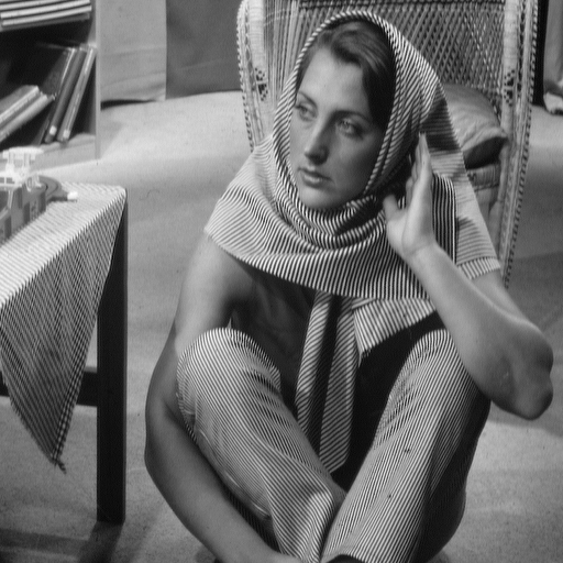
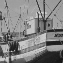
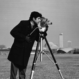
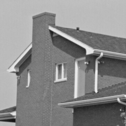
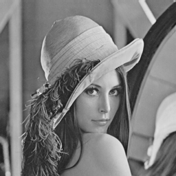
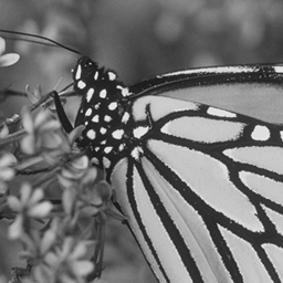
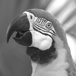
Figure 1: Images used for CS experiment, {barbara, boat, cameraman, foreman, house, lena, monarch, parrot}.

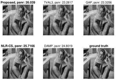
Figure 2: Reconstruction results of different algorithms at CSr$=0.1$, image size $256\times 256$.

Following the formulation of the lensless camera [5], the permuted Hadamard matrix is used as the sensing matrix. Each image is resized to $256\times 256$ and these images are shown in Figure 1. The CSr is defined as:

$$\text{CSr}=\frac{{\text{number of rows in }}{\bf A}}{{\text{number of columns in }}{\bf A}}$$ (75)

where the number of columns in ${\bf A}$ is equivalent to the total pixel number of the image. The sensing matrix is constructed from rows of a Hadamard matrix of order $N=2^{16}$. The columns of the Hadamard matrix is permuted according to a predetermined random permutation (the same permutation is used in the real data captured by our lensless camera). For each CSr, we use the first CSr$\times N$ rows of the column-permuted Hadamard matrix as the sensing matrix. By selecting some other rows of the permutated Hadamard matrix, we can get better results [47]. However, here we just select the top rows to be consistent to the implementation of our lensless camera. Note that in this case, ${\bf A}{\bf A}^{\top}$ is an identity matrix and it is very fast to use accelerated GAP update for $\boldsymbol{x}$ in (67). We observed that best results are obtained by the LR-GMM-SLOPE with GAP updates of $\boldsymbol{x}$ and these results are reported in this section. For the comparison of IST, GAP and ADMM, please refer to Section V-B.

Since when CSr=0.1, good results have been achieved for most images (see Figure 2 for one example), we here spend more efforts on the extremely low CSr, in particular CSr$<0.1$, which may be of interest to the real applications that are used to detect anomalous events [48] without caring too much about the image quality. The results are summarized in Table I. We can observe that best results are obtained by the proposed aglorithm, NLR-CS or D-AMP. When CSr is less than 0.1, the proposed algorithm usually provides best results except “foreman”, where NLR-CS is the best. We also observed that NLR-CS is very sensitive to the parameters and sometimes the PSNRs are not linearly increasing as the CSr increases, while the other algorithms including the proposed do not have this problem. On average, our proposed algorithm works best when CSr$\leq 0.1$. Though did not reported here, when CSr$>0.1$, the proposed algorithm also provides comparable or better results than D-AMP and NLR-CS. But we need to tune the noise parameter used in $\boldsymbol{n}$, while for all the results presented here, we set it to the same value ${{\bf E}}=10^{-5}{\bf I}$. In addition, we need to tune the rank thresholds $\gamma_{k}$, for which we have observed that a higher CSr requires a larger $\gamma_{k}$.

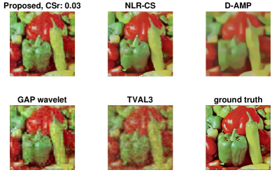
Figure 3: Reconstruction results of different algorithms at CSr$=0.03$.

In addition to the grayscale images tested above as in other papers, we also conduct our proposed algorithm on the RGB images with results shown in Table II. Three sensors are simulated to capture the R, G and B components of the image. The “book” scene corresponds to the real data captured by our lensless camera. Again, our proposed algorithm provides the best results. One example with CSr$=0.03$ is shown in Figure 3. It can be seen that our algorithms provide more details than NLR-CS and D-AMP; both of them presents “blob” artifacts.

V-A Compare to JPEG Compression

TABLE III: JPEG compression at different qualities compared with the proposed compressive sensing recovery

JPEG Compression			CS Reconstruction		Difference
	Size	PSNR		PSNR	PSNR
Quality	(bytes)	(dB)	CSr	(dB)	(dB)
1	1,563	22.0683	0.0334	22.1507	-0.0823
3	1,716	22.7278	0.0367	22.4125	0.3154
5	2,153	24.8416	0.0460	23.2433	1.5983
7	2,559	26.0924	0.0547	23.8426	2.2548
9	2,946	26.9623	0.0630	24.3308	2.6315
10	3,141	27.2853	0.0672	24.5945	2.6908
12	3,494	27.8379	0.0747	24.9514	2.8866
14	3,815	28.2981	0.0816	25.3233	2.9748
16	4,160	28.6912	0.0890	25.6880	3.0032
18	4,478	29.0306	0.0958	25.9230	3.1077
20	4,752	29.3411	0.1016	26.1267	3.2144

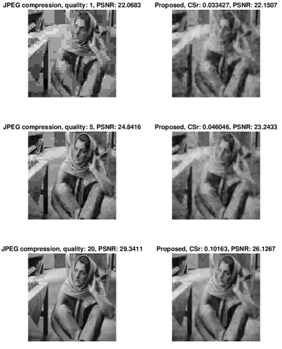
Figure 4: Example images: JPEG compared with the proposed algorithm.

We now compare LR-GMM-SLOPE under the compressive sensing framework with the JPEG compression, which is based on the sparsity of the DCT coefficients of $8\times 8$ blocks (non-overlapping patches). We first use an PNG file as the ground truth and then use the script within MATLAB “imwrite($\cdot$)” by choosing 8-bits ‘jpeg’ compression with different qualities (100 denotes the highest quality). We treat the quality 100 as the standard full file size. For the ‘Barbara’ image we used here, PSNR = 58.47dB (w.r.t. the PNG file) and the file size is 45.6KB at quality 100. The compressed image is obtained by changing the compression quality from 1 to 100 and we compare the file size with the full size at quality 100, computing the CSr used in this paper.

Table III summarizes the results of JPEG compression compared with the results obtained by our algorithm. This is a rough, high level comparison because JPEG also performs an entropy encoding after the DCT transform and quantization, while in our method, the number of compressive measurements is compared with the number of total pixels, and we did not consider the entropy coding on quantized measurements. We intend to take the effect of the entropy encoding in JPEG out of the comparison by computing the JPEG compression ratio as compared to the quality 100. When the compression is high (lower CSr), the gap between our approach and the JPEG compression is small. It is worth noting that when CSr=0.0334, our algorithm performs better than JPEG. When the compression gets lower, the gap becomes larger. One possible reason is that when JPEG is performed on the image, the ground truth is available and it is very easy to capture useful information from the truth. However, under the compressive sensing framework and using the current algorithm, increasing a few number of measurements can help the reconstruction, but not that significantly. Example images can be found in Figure 4. It can be seen that JPEG compression has obvious block artifacts while the results of the proposed algorithm become better progressively with increasing number of measurements.

Furthermore, in JPEG compression, if we lose some bits, we may not be able to decode entire blocks. By contrast, in our compressive sensing framework, if we lose some measurements, we can still reconstruct the image, maybe not at a high fidelity.

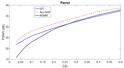
Figure 5: One example (parrot) to compare different updating rules (IST, Acc-GAP, ADMM) of $\boldsymbol{x}$.

V-B Comparison of Different Update Rules for $\boldsymbol{x}$

We provide three approaches in Section IV-A to update $\boldsymbol{x}$ in order to minimize the objective function in (63). Now we compare these three updates via experiments. We emphasize again that we are using the permuted Hadamard matrix as the sensing matrix and thus ${\bf A}{\bf A}^{\top}$ is an identity matrix. Therefore, updating $\boldsymbol{x}$ via GAP in (66) is same as updating $\boldsymbol{x}$ via IST in (65). However, the accelerated GAP in (67) provides best results in our experiments. Without tunning the ADMM parameters carefully, we compare these three update methods with different images at various CSr, and one example is shown in Figure 5. It can be observed that the accelerated GAP update always provides the best result and when CSr is low, IST is better than ADMM. When CSr is getting larger, ADMM becomes better than IST. Because of this, all the results reported in this paper is generated by the accelerated GAP update.

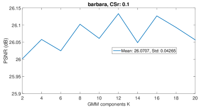
Figure 6: Reconstruction PSNR with different number of GMM components ($K$). Barbara is used with CSr = 0.1.

V-C Different Number of Gaussian Mixture Components

One problem of using GMM is how to set the component number $K$. As we are using the mixture model, each patch is represented by the posterior distribution, another GMM. Therefore, selecting this $K$ is not as critical as in the PLE [41]. An alternative way to infer this $K$ is utilizing the manifold factor analysis model as developed in [44]. Hereby, we investigate this point empirically by using the “barbaba” image as used before with different number of $K\in[2,20]$. The results at CSr$=0.1$ are shown in Figure 6. It can be seen that our algorithm is not sensitive to this $K$, since the standard deviation of the PSNRs with different $K$ is only 0.04265dB compared with the mean value 26.0707dB.

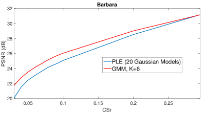
Figure 7: One example (barbara) to compare LR-PLE-SLOPE (20 Gaussian models) with LR-GMM-SLOPE ($K=6$).

V-D GMM vs. PLE and Computational Time

As mentioned earlier, when we consider that each patch is drawn from a single Gaussian component, the proposed approach degrades to the PLE. We verify the performance of LR-PLE-SLOPE compared with the LR-GMM-SLOPE in Figure 7. It can be seen that the GMM always performs better than the PLE at lower CSr. When CSr is getting larger, they start to perform similarly.

Regrading the computational time, our algorithm is similar to NLR-CS. If a warm start is used to initialize the $\hat{\boldsymbol{x}}$, we can obtain a good reconstruction within 20 iterations. One $256\times 256$ grayscale image reconstruction at CSr$=0.1$ takes around 1 minute on an i7CPU with 24G RAM. Similar time is required for the LR-PLE-SLOPE but it needs more memory. While the most time consumption of LR-GMM-SLOPE is the EM training of GMM, the LR-PLE-SLOPE requires a long time for the model selection, and it usually needs more Gaussian components (i.e., 20) than the GMM to get good results.

VI Real Data Results for the Lensless Camera

We now verify our proposed algorithm on the real data captured by our lensless camera [5], which is composed of an aperture assembly and a single sensor (a photodiode) to capture grayscale images; it can also be a RGB sensor to capture color images. The aperture assembly implements the sensing matrix and we programmed it to be the permuted Hadamard matrix. By capturing the scene with different sensing matrices, we obtain the measurement vector $\boldsymbol{y}$. We implemented the aperture assembly with a transparent LCD and thus we can control the image resolution by merging the neighboring pixels.

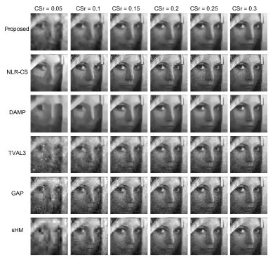
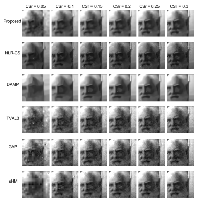
Figure 8: Real data: reconstruction results at different CSr with the diverse algorithms. The image is of size $128\times 128$. Two photos (top: Lena, bottom: Alexander Graham Bell) are used as the scene.

VI-A Gray-Scale Images

We first consider the case with gray scale sensor and the image resolution of $128\times 128$. To capture compressive measurements, we use a sensing matrix which is constructed from rows of a Hadamard matrix of order $N=2^{14}$. Each row of the Hadamard matrix is permuted according to a predetermined random permutation. The scene is composed of a photo printed on a paper and we capture the measurements of this photo. Example results using different numbers of measurement are shown in Fig. 8. We also compare the five algorithms used in the simulation. It can be seen that, similar to the simulation, our proposed algorithm provides best result when CSr is small. Especially, at CSr = 0.05 and 0.1, our algorithm can present many details of the face, for example, the left eye of “Lena”. D-AMP introduces some “blob” noise because the BM3D denoising approach is used. Though NLR-CS can provide good results at CSr = 0.05 and 0.1, it introduces some unpleasant artifacts when CSr is from 0.15 to 0.25. We also tried the algorithm (sHM) proposed in [49], where a Bayesian model is developed to investigate the tree-structure in wavelet. Surprisingly, sHM now works better than TVAL3 and GAP, mainly due to the following two reasons. Firstly, the tree structure in wavelet helps the reconstruction and secondly, the Bayesian framework developed in [49] is very robust to noise; it infers noise from the measurements.

Figure 9: Real data: reconstruction results at different CSr with the proposed algorithm. The image is of size $217\times 302\times 3$.

VI-B RGB Images

Next we consider the RGB images captured by the RGB sensor, and now the resolution is $217\times 302\times 3$. The sensing matrix is constructed from rows of a Hadamard matrix of order $N=2^{16}$ and the first $65534$ elements are used. The scene is the real scene of four books as shown [5, 20]. The reconstruction result is shown in Figure 9 with diverse CSr.

Note that by using compressive measurements, we can save the sensors as well as the bandwidth. As stated earlier, we may progressively get better results by receiving more measurements. One of the main usage of compressive sensing is to get features in limited data by using a small bandwidth. From the results in Figure 8, we may identity high quality features from the reconstructed image at CSr around 0.1. If we want to get some details, for example, the book titles in Figure 9, we may need CSr around 0.2. On the other hand, if we only need to identify that these are “books” in Figure 9, CSr at 0.05 may be sufficient.

VII Conclusions

A novel compressive sensing reconstruction algorithm is developed via exploiting the low-rank property of overlapping patches. A general iteratively two-step framework for compressive sensing recovery is proposed. A denoising operator is used to update the estimate of the desired image (obtained by the projection of the measurements), which can be implemented by investigating the sparsity or low-rank property of the image patches. We develop a probabilistic regime by representing each patch via a Gaussian mixture model and impose low-rank on each Gaussian component to achieve the state-of-the-art compressive sensing reconstruction results, in particular when the measurement number is small. Additionally, the proposed low-rank GMM algorithm degrades to the low-rank piecewise linear estimator if each patch is modeled by a single Gaussian model. Extensive results on both simulation and real data demonstrate high performance of the proposed algorithm.

References

- [1] D. L. Donoho, “Compressed sensing,” IEEE Transactions on Information Theory, vol. 52, no. 4, pp. 1289–1306, April 2006.
- [2] E. J. Candès, J. Romberg, and T. Tao, “Robust uncertainty principles: Exact signal reconstruction from highly incomplete frequency information,” IEEE Transactions on Information Theory, vol. 52, no. 2, pp. 489–509, February 2006.
- [3] E. J. Candès and M. B. Wakin, “An introduction to compressive sampling,” IEEE Signal Processing Magazine, vol. 25, no. 2, pp. 21–30, March 2008.
- [4] R. Baraniuk, “Compressive sensing,” IEEE Signal Processing Magazine, vol. 24, no. 4, pp. 118–121, July 2007.
- [5] G. Huang, H. Jiang, K. Matthews, and P. Wilford, “Lensless imaging by compressive sensing,” IEEE International Conference on Image Processing, 2013.
- [6] X. Yuan, H. Jiang, G. Huang, and P. Wilford, “Lensless compressive imaging,” arXiv:1508.03498, 2015.
- [7] P. Llull, X. Liao, X. Yuan, J. Yang, D. Kittle, L. Carin, G. Sapiro, and D. J. Brady, “Coded aperture compressive temporal imaging,” Optics Express, pp. 698–706, 2013.
- [8] X. Yuan, P. Llull, X. Liao, J. Yang, G. Sapiro, D. J. Brady, and L. Carin, “Low-cost compressive sensing for color video and depth,” in IEEE Conference on Computer Vision and Pattern Recognition (CVPR), 2014.
- [9] X. Yuan, J. Yang, X. Liao, P. Llull, G. Sapiro, D. J. Brady, and L. Carin, “Adaptive temporal compressive sensing for video,” IEEE International Conference on Image Processing, pp. 1–4, 2013.
- [10] X. Yuan and S. Pang, “Structured illumination temporal compressive microscopy,” in Frontier in Optics (FiO), 2015.
- [11] A. Stevens, L. Kovarik, P. Abellan, X. Yuan, L. Carin, and N. D. Browning, “Applying compressive sensing to tem video: A substantial framerate increase on any camera,” Advanced Structural and Chemical Imaging, 2015.
- [12] P. Llull, X. Yuan, X. Liao, J. Yang, L. Carin, G. Sapiro, and D. Brady, “Compressive extended depth of field using image space coding,” in Computational Optical Sensing and Imaging (COSI), 2014, pp. 1–3.
- [13] A. Wagadarikar, R. John, R. Willett, and D. J. Brady, “Single disperser design for coded aperture snapshot spectral imaging,” Applied Optics, vol. 47, no. 10, pp. B44–B51, 2008.
- [14] X. Yuan, T.-H. Tsai, R. Zhu, P. Llull, D. J. Brady, and L. Carin, “Compressive hyperspectral imaging with side information,” IEEE Journal of Selected Topics in Signal Processing, vol. 9, no. 6, pp. 964–976, September 2015.
- [15] T.-H. Tsai, P. Llull, X. Yuan, D. J. Brady, and L. Carin, “Spectral-temporal compressive imaging,” Optics Letters, vol. 40, no. 17, pp. 4054–4057, Sep 2015.
- [16] T.-H. Tsai, X. Yuan, and D. J. Brady, “Spatial light modulator based color polarization imaging,” Optics Express, vol. 23, no. 9, pp. 11 912–11 926, May 2015.
- [17] W. L. Chan, K. Charan, D. Takhar, K. F. Kelly, R. G. Baraniuk, and D. M. Mittleman, “A single-pixel terahertz imaging system based on compressed sensing,” Applied Physics Letters, vol. 93, no. 12, pp. 121 105––121 105––3, 2008.
- [18] S. Babacan, M. Luessi, L. Spinoulas, A. Katsaggelos, N. Gopalsami, T. Elmer, R. Ahern, S. Liao, and A. Raptis, “Compressive passive millimeter-wave imaging,” International Conference on Image Processing, pp. 2705–2708, 2011.
- [19] J. Yang, X. Liao, X. Yuan, P. Llull, D. J. Brady, G. Sapiro, and L. Carin, “Compressive sensing by learning a Gaussian mixture model from measurements,” IEEE Transaction on Image Processing, vol. 24, no. 1, pp. 106–119, January 2015.
- [20] H. Jiang, G. Huang, and P. Wilford, “Multi-view in lensless compressive imaging,” APSIPA Transactions on Signal and Information Processing, vol. 3, no. 15, pp. 1–10, 2014.
- [21] M. A. T. Figueiredo, R. D. Nowak, and S. J. Wright, “Gradient projection for sparse reconstruction: Application to compressed sensing and other inverse problems,” pp. 586–597, Dec. 2007.
- [22] M. A. Figueiredo, J. M. Bioucas-Dias, and R. D. Nowak, “Majorization–minimization algorithms for wavelet-based image restoration,” IEEE Transactions on Image Processing, vol. 16, no. 12, pp. 2980–2991, 2007.
- [23] W. Yin, S. Osher, D. Goldfarb, and J. Darbon, “Bregman iterative algorithms for -minimization with applications to compressed sensing,” SIAM J. Imaging Sci, pp. 143–168, 2008.
- [24] E. Candes, M. Wakin, and S. Boyd, “Enhancing sparsity by reweighted minimization,” Journal of Fourier Analysis and Applications, vol. 14, no. 5, pp. 877–905, 2008.
- [25] J. A. Tropp and A. C. Gilbert, “Signal recovery from random measurements via orthogonal matching pursuit,” IEEE Transactions on Information Theory, 2007.
- [26] I. Daubechies, R. DeVore, M. Fornasier, and C. S. Güntürk, “Iteratively reweighted least squares minimization for sparse recovery,” Communications on Pure and Applied Mathematics, vol. 63, no. 1, pp. 1–38, 2010.
- [27] J. Bioucas-Dias and M. Figueiredo, “A new TwIST: Two-step iterative shrinkage/thresholding algorithms for image restoration,” IEEE Transactions on Image Processing, vol. 16, no. 12, pp. 2992–3004, December 2007.
- [28] S. Ji, Y. Xue, and L. Carin, “Bayesian compressive sensing,” IEEE Transactions on Signal Processing, vol. 56, no. 6, pp. 2346–2356, June 2008.
- [29] L. He and L. Carin, “Exploiting structure in wavelet-based bayesian compressive sensing,” IEEE Transactions on Signal Processing, vol. 57, no. 9, pp. 3488–3497, September 2009.
- [30] C. Li, W. Yin, H. Jiang, and Y. Zhang, “An efficient augmented lagrangian method with applications to total variation minimization,” Computational Optimization and Applications, vol. 56, no. 3, pp. 507–530, 2013.
- [31] Y. Huang, J. Paisley, Q. Lin, X. Ding, X. Fu, and X. Zhang, “Bayesian nonparametric dictionary learning for compressed sensing MRI,” IEEE Transactions on Image Processing, vol. 23, no. 12, pp. 5007–5019, December 2014.
- [32] S. D. A. Averbuch and S. Deutsch, “Adaptive compressed image sensing using dictionaries,” SIAM Journal on Imaging Sciences, vol. 5, no. 1, pp. 57–89, 2012.
- [33] W. Dong, G. Shi, X. Li, Y. Ma, and F. Huang, “Compressive sensing via nonlocal low-rank regularization,” IEEE Transactions on Image Processing, vol. 23, no. 8, pp. 3618–3632, 2014.
- [34] C. A. Metzler, A. Maleki, and R. G. Baraniuk, “From denoising to compressed sensing,” arXiv:1406.4175, 2014.
- [35] A. Beck and M. Teboulle, “A fast iterative shrinkage-thresholding algorithm for linear inverse problems,” SIAM J. Img. Sci., vol. 2, no. 1, pp. 183–202, Mar. 2009.
- [36] X. Liao, H. Li, and L. Carin, “Generalized alternating projection for weighted- minimization with applications to model-based compressive sensing,” SIAM Journal on Imaging Sciences, vol. 7, no. 2, pp. 797––823, 2014.
- [37] S. Boyd, N. Parikh, E. Chu, B. Peleato, and J. Eckstein, “Distributed optimization and statistical learning via the alternating direction method of multipliers,” Found. Trends Mach. Learn., vol. 3, no. 1, pp. 1–122, January 2011.
- [38] K. Dabov, A. Foi, V. Katkovnik, and K. Egiazarian, “Image denoising by sparse 3d transform-domain collaborative filtering,” IEEE Transactions on Image Processing, vol. 16, no. 8, pp. 2080–2095, August 2007.
- [39] M. Elad and M. Aharon, “Image denoising via sparse and redundant representations over learned dictionaries,” IEEE Transactions on Image Processing, vol. 15, pp. 3736––3745, December 2006.
- [40] G. Yu and G. Sapiro, “Statistical compressed sensing of Gaussian mixture models,” IEEE Transactions on Signal Processing, vol. 59, no. 12, pp. 5842–5858, 2011.
- [41] G. Yu, G. Sapiro, and S. Mallat, “Solving inverse problems with piecewise linear estimators: From Gaussian mixture models to structured sparsity,” IEEE Transactions on Image Processing, 2012.
- [42] H. Jiang, G. Huang, P. A. Wilford, and L. Yu, “Constrained and preconditioned stochastic gradient method,” IEEE Transactions on Signal Processing, vol. 63, no. 10, pp. 2678–2691, 2015.
- [43] J. Yang, X. Yuan, X. Liao, P. Llull, G. Sapiro, D. J. Brady, and L. Carin, “Video compressive sensing using Gaussian mixture models,” IEEE Transaction on Image Processing, vol. 23, no. 11, pp. 4863–4878, November 2014.
- [44] M. Chen, J. Silva, J. Paisley, C. Wang, D. Dunson, and L. Carin, “Compressive sensing on manifolds using a nonparametric mixture of factor analyzers: Algorithm and performance bounds,” IEEE Transactions on Signal Processing, vol. 58, no. 12, pp. 6140–6155, December 2010.
- [45] A. Gut, An Intermediate Course in Probability. Springer, 2009.
- [46] J.-F. Cai, E. J. Candès, and Z. Shen, “A singular value thresholding algorithm for matrix completion,” SIAM J. on Optimization, vol. 20, no. 4, pp. 1956–1982, Mar. 2010.
- [47] J. Romberg, “Imaging via compressive sampling,” IEEE Signal Processing Magazine, vol. 25, no. 2, pp. 14–20, 2008.
- [48] H. Jiang, W. Deng, and Z. Shen, “Surveillance video processing using compressive sensing,” Inverse Problems and Imaging, vol. 5, no. 2, pp. 201–214, 2012.
- [49] X. Yuan, V. Rao, S. Han, and L. Carin, “Hierarchical infinite divisibility for multiscale shrinkage,” IEEE Transactions on Signal Processing, vol. 62, no. 17, pp. 4363–4374, Sep. 1 2014.