On the Hamiltonian Number of a Planar Graph

Abstract.

The Hamiltonian number of a connected graph is the minimum of the lengths of the closed, spanning walks in the graph. In 1968, Grinberg published a necessary condition for the existence of a Hamiltonian cycle in a planar graph, formulated in terms of the lengths of its face cycles. We show how Grinberg’s theorem can be adapted to provide a lower bound on the Hamiltonian number of a planar graph.

1. Introduction

A Hamiltonian cycle in a graph is a closed, spanning walk that visits each vertex exactly once; a graph is called Hamiltonian provided that it contains a Hamiltonian cycle. While not every graph is Hamiltonian, every connected graph contains a closed, spanning walk. A closed, spanning walk of minimum length is called a Hamiltonian walk, and the Hamiltonian number of a connected graph $G$, denoted by $h(G)$, is the length of a Hamiltonian walk in $G$. Thus the Hamiltonian number of a graph can be understood as a measure of how far the graph deviates from being Hamiltonian.

In 1968, Grinberg [11] published a necessary condition for the existence of a Hamiltonian cycle in a planar graph, formulated in terms of the lengths of its face cycles. The sole purpose of this paper is to show how Grinberg’s theorem can be adapted to provide a lower bound on the Hamiltonian number of a planar graph. Before we state this theorem, it is helpful to place our work in context.

In general, determining the Hamiltonian number of a graph is difficult, but for a connected graph $G$ of order $n$, the elementary bounds

$$n\leq h(G)\leq 2(n-1)$$

are easily obtained. A Hamiltonian walk on $G$ must visit each vertex, which gives the lower bound. On the other hand, a pre-order, closed, spanning walk on a spanning tree of $G$ has length $2(n-1)$, yielding the upper bound. Over the years, much of the research on the Hamiltonian number has advanced along two fronts: developing tighter bounds for the Hamiltonian number in terms of natural graph parameters, or evaluating the Hamiltonian numbers of some special graphs or families of graphs.

Goodman and Hedetniemi [9] initiated the study of the Hamiltonian number of a graph. They proved, among other things, properties of Hamiltonian walks, upper and lower-bounds for the Hamiltonian number of a graph, and a formula for the Hamiltonian number of a complete $n$-partite graph. Their most accessible result is this: let $G$ be a $k$-connected graph on $n$ vertices with diameter $d$; then

$$h(G)\leq 2(n-1)-\lfloor k/2\rfloor(2d-2),$$

which improves the elementary upper bound. In another result, they related the Hamiltonian numbers of $G$ and $G-U$ , the graph obtained by deleting the unicliqual points of G.

Soon after the publication of the seminal paper of Goodman and Hedetniemi, Bermond [3] published a theorem on the Hamiltonian number problem inspired by Ore’s theorem. Ore’s theorem gives a sufficient condition for a graph to be Hamiltonian in terms of the sums of the degrees of non-adjacent vertices; see, for example, Theorem 6.6 of [7]. Bermond showed the following: let $G$ be a graph of order $n$ and let $c\leq n$; if $\deg(v)+\deg(w)\geq c$ for every pair of non-adjacent vertices $v$ and $w$ in $V(G)$, then $h(G)\leq 2n-c.$

Chartrand, Thomas, Zhang, and Saenpholphat [8] introduced an alternative approach to the Hamiltonian number. Let $G$ be a connected graph of order $n$. Given vertices $u$ and $v$, let $d(u,v)$ denote the length of a shortest path from $u$ to $v$. A cyclic ordering of the vertices of $G$ is a permutation $s:v_{1},v_{2},\ldots,v_{n},v_{n+1}$ of $V(G)$, where $v_{n+1}=v_{1}$. Given a cyclic ordering $s$, let $d(s)=\sum_{i=1}^{n}d(v_{i},v_{i+1})$. The set

$$H(G)=\{d(s):\text{$s$ is a cyclic ordering of $V(G)$}\}$$

is called the Hamiltonian spectrum of $G$. Chartrand and his colleagues showed that $h(G)=\min H(G).$ This paper contains two other notable results: first, that a connected graph $G$ of order $n$ satisfies $h(G)\leq 2(n-1)$ with equality if and only if $G$ is a tree; second, that for each integer $n\geq 3$, every integer in the interval $[n,2(n-1)]$ is the Hamiltonian number of some graph of order $n$. Král, Tong, and Zhu [12] and Liu [13] conducted additional research on the Hamiltonian spectra of graphs.

Various authors have studied the Hamiltonian number of special graphs and families of graphs. Punnim and Thaithae [19, 17] studied the Hamiltonian numbers of cubic graphs. A graph of order $n$ with Hamiltonian number $n+1$ is called almost Hamiltonian. Punnim, Saenpholphat, and Thaithae [16] characterized the almost Hamiltonian cubic graphs and the almost Hamiltonian generalized Petersen graphs. Asano, Nishizeki, and Watanabe [2, 14] established a simple upper bound for the Hamiltonian number of a maximal planar graph of order $n\geq 3$ and created an algorithm for finding closed, spanning walks in a graph with length close to its Hamiltonian number. G. Chang, T. Chang, and Tong [5] studied the Hamiltonian numbers of Möbius double loop networks. The Hamiltonian number problem has a variety of cognates: Vacek [20, 21] analyzed open Hamiltonian walks; Araya and Wiener [1, 22] investigated hypohamiltonian graphs; Goodman, Hedetniemi, and Slater [10] studied the the Hamiltonian completion problem; T. Chang and Tong [6] considered the Hamiltonian numbers of strongly connected digraphs; and, Okamoto, Zhang, and Saenpholphat [18, 15] studied the upper traceable numbers of graphs.

2. The Grinberg number of a planar graph

Let $G$ be a planar graph and let the faces (including the unbounded component) be labeled $F_{1},F_{2},\ldots,F_{N}$. Given a face $F$, let $|F|$ denote its length, that is, the number of its edges (or vertices). Let $\mathscr{G}(G)$ be the set of all sums of the form

$$\left|\sum_{i=1}^{N}\varepsilon_{i}(|F_{i}|-2)\right|$$

where $(\varepsilon_{1},\varepsilon_{2},\ldots,\varepsilon_{N})\in\{1,+1\}^{N}$, excluding the two cases where all of the components have the same sign. Let $g(G)=\min\mathscr{G}(G).$ will call $\mathscr{G}(G)$ the Grinberg set of $G$ and $g(G)$ the Grinberg number of $G$. To develop a feel for this, consider the graph presented in Figure 1. This graph has five interior faces, each a hexagon, and the exterior face has 18 edges. The Grinberg set for this graph is $\{4,12,20,28\}$ and the Grinberg number is 4.

Figure 1. A graph with Grinberg set $\{4,12,20,28\}$ an Grinberg number 4.

Grinberg’s theorem can be stated as follows: if a planar graph $G$ is Hamiltonian, then $g(G)=0$; see [11]. Our main result can be seen as a natural extension of Grinberg’s theorem.

Theorem 2.1.

Let G be a planar graph. A closed, spanning walk on G must contain $g(G)/2$ repeats of vertices.

Proof.

Our proof is an adaptation of the customary proof of Grinberg’s theorem; see, for example, Theorem 18.2 of [4]. Let the vertices of the planar graph $G$ be labeled $\{v_{1},v_{2},...,v_{n}\}$ and let $\sigma$ be a closed, spanning walk on $G$, given as a list of these vertices. First we will produce a new planar multigraph $G^{\prime}$, called the reduction of $G$, relative to $\sigma$. The reduced graph is created through applications of the following procedures:

Edge removal:

Remove any edge from $G$ that was not traversed by $\sigma$.

Edge duplication:

If an edge of $G$ is traversed more than once by $\sigma$, then create an additional edge in $G^{\prime}$ for each additional traversal of this edge by this walk.

Thus, while the reduced graph $G^{\prime}$ is still planar, it may no longer be simple. The faces of $G^{\prime}$ are labeled with a $+$ or a $-$ sign as follows: the unbounded component is marked $+$; thereafter, if a face of $G^{\prime}$ is adjacent to (shares an edge with) a $+$ region, then it is marked $-$, and if a face of $G^{\prime}$ is adjacent to a $-$ region, then it is marked $+$. An example of a planar graph and its reduction relative to a closed, spanning walk is presented in Figure 2.

Figure 2. A planar graph (left) and its reduction (right) based on the closed, spanning walk $a,b,c,d,e,f,g,h,a,i,j,r,j,k,l,m,n,p,q,p,n,o,a$. Notice that the reduced graph has 4 repeated vertices and 6 faces.

There is a simple relationship between the number of faces of $G^{\prime}$ and the number of repeats of vertices in the closed, spanning walk $\sigma$. For each $i$, $1\leq i\leq n$, let $m_{i}$ count the number of times vertex $v_{i}$ is repeated in the walk $\sigma$. To be clear about this, if the vertex $v_{i}$ appears only once in the walk $\sigma$, then $m_{i}=0$. Let $\Phi$ count the number of faces of the reduced graph $G^{\prime}$. By way of the Euler characteristic formula, we will show that

(1) $$\Phi=2+\sum_{i=1}^{n}m_{i}.$$

The degree of the vertex $v_{i}$ is $2m_{i}+2$ and therefore the number of edges of $G^{\prime}$ is half of the sum of the degrees taken over all vertices, that is $\sum_{i=1}^{n}(m_{i}+1).$ Thus

$$n-\sum_{i=1}^{n}(m_{i}+1)+\Phi=2,$$

from which formula (1) follows.

Our argument now moves into a second phase, culminating in a simple formula relating the lengths of the positively and negatively signed faces of $G^{\prime}$. Let the faces of $G^{\prime}$ be divided according to their signs and let $\{A^{+}:1\leq n_{+}\}$ be the labels for the positively signed faces and let $\{A^{-}:1\leq n_{-}\}$ be the labels for the negatively signed faces. Since each edge of $G^{\prime}$ is adjacent to a positively and a negatively signed face, it follows that

$$\sum_{i=1}^{n_{+}}|A^{+}|=\sum_{i=1}^{n_{-}}|A^{-}|.$$

Let $\Delta=n_{-}-n_{+}$, the difference between the number of negatively and positively signed faces of $G^{\prime}$. Then

(2) $$\left|\sum_{i=1}^{n_{+}}(|A^{+}|-2)-\sum_{i=1}^{n_{-}}(|A^{-}|-2)\right|=2|\Delta|.$$

We will modify this formula to incorporate the faces of $G$. Let the faces of $G$ be labeled $\{F_{i}:1\leq i\leq N\}$. Each face of $G$ is contained by a unique face of $G^{\prime}$. For each $i$, $1\leq i\leq N$, let $\varepsilon_{i}$ be sign of the face of $G^{\prime}$ that contains $F_{i}$. We will show that

(3) $$\left|\sum_{i=1}^{N}\varepsilon_{i}(|F_{i}|-2)\right|=2|\Delta|.$$

To verify this claim, we will follow Grinberg’s strategy: we will add to $G^{\prime}$ , one at a time, those edges of G that were not traversed by $\sigma$. Such an edge must split a face of $G^{\prime}$ into two sub-faces, each with the same sign as the parent face. For the sake of argument, let us say that a face labeled $A_{i}^{+}$ is divided by an edge of $G$ into two sub-faces, labeled $A_{i_{1}}^{+}$ and $A_{i_{2}}^{+}$. Since the two sub-faces share exactly one edge, we have

$$|A_{i}^{+}|-2=(|A_{i_{1}}^{+}|-2)+(|A_{i_{2}}^{+}|-2).$$

Hence we can substitute $(|A_{i_{1}}^{+}|-2)+(|A_{i_{2}}^{+}|-2)$ for $|A_{i}^{+}|-2$ in equation (2) and retain equality. We continue this process until all of these edges have been added. We have almost arrived at equation (3). The only difference corresponds to those faces of $G^{\prime}$ that were created because an edge was traversed more than once by $\sigma$, the closed, spanning walk. Such a face has only two edges and thus contributes 0 in the sum. In this way, we have transformed equation (2) into equation (3).

Our proof is nearly complete. By the definition of the Grinberg number of a graph and equation (3),

$$g(G)\leq\left|\sum_{i=1}^{N}\varepsilon_{i}(|F_{i}|-2)\right|=2|\Delta|$$

Recall that $n_{-}$ and $n_{+}$ count the number of negatively and positively signed faces in $G^{\prime}$, respectively, and each of these must be at least 1. Since they sum to $\Phi$, it must be that $|\Delta|\leq\Phi-2$. Bearing in mind equation (1), we obtain

$$\frac{1}{2}g(G)\leq\sum_{i=1}^{n}m_{i},$$

as was to be shown. ∎

3. Some examples

In this section we present several examples of Theorem 2.1.

1. The graph in Figure 1 has Grinberg number 4; thus, any closed, spanning walk on this graph must have two repeats of vertices. It is easy to find a closed, spanning walk with two repeats and thus this is optimal.

2. Consider the simple grid graph presented in Figure 3. The exterior face has 8 edges; each of the four interior faces has 4 edges. The Grinberg number of this graph is 2, and any closed, spanning walk on this graph must contain at least one repeated vertex. It is easy to find an example of a closed, spanning walk with one repeated vertex.

   Figure 3. A simple grid graph with Grinberg number 2.

3. The Grinberg number of a tree can be computed by duplicating each edge and computing the Grinberg number of the resulting planar graph. The altered version of the tree in Figure 4 has an outside face with 20 edges and 10 interior faces with 2 edges each. The Grinberg number of this tree is 18 and any closed, spanning walk on this tree must contain at least 9 repeats of vertices.

   Figure 4. A tree and its alteration.

4. The graph presented in Figure 5 has an outside face with 26 edges and three interior faces, each with 14 edges. The Grinberg number is 12; thus, any closed, spanning walk on this graph must have at least 6 repeats. It is easy to find a closed, spanning walk with 6 repeats. For example, begin at $a$ and walk around the outside of the graph, ending at $a$. Now augment the walk by adding $a,b,c,d,c,b,a,e,f,g,f,e,a$. This walk has 6 repeats of vertices: $a$ (twice), $b$, $c$, $e$, and $f$.

   Figure 5. A graph with Grinberg number 12. A closed, spanning walk on this graph must have at least 6 repeats of vertices.

5. Figure 6 exhibits a graph with 8 interior faces, each an octagon, and an exterior face with 20 edges. The Grinberg number of this graph is 6. Any closed, spanning walk on this graph must have at least 3 repeats of vertices. A closed, spanning walk with exactly 3 repeats is pictured in the figure.

   Figure 6. The graph on the left has Grinberg number 6. A Hamiltonian walk on this graph (with 3 repeats) is shown on the right.

4. Additional observations

Given a closed, spanning walk on the planar graph $G$, let $\rho$ count the number of repeats of vertices, let $\nu=n^{-}-1$, and let $\pi=n_{+}-1$. In other words, $\nu$ is one less than the number of negatively signed regions in $G^{\prime}$ and $\pi$ is one less than the number of its positively signed regions in $G^{\prime}$.

Since the reduced graph must have at least one of each type of each signed region, $\nu$ and $\pi$ are nonnegative. By equations (1) and (3), there exists an element $f\in\mathscr{G}(G)$ for which

$$f =\nu+\pi$$

$$\frac{1}{2}f =\max\{\nu,\pi\}-\min\{\nu,\pi\}$$

In particular, this shows that

$$\rho=\frac{1}{2}f+2\min\{\nu,\pi\}.$$

This can be a helpful observation when searching for Hamiltonian walks. For example, consider a planar graph $G$ with 8 interior faces, each an octagon, and an exterior face with 20 edges. The Grinberg set for this graph is $\{6,18,30,42,54\}$; hence, the number of repeats of vertices in a Hamiltonian walk on G must be at least 3 and odd. The graph pictured in Figure 6 has a Hamiltonian walk with the minimal number of repeats, while the graph pictured in Figure 7 has a Hamiltonian walk that requires 5 repeats.

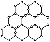
Figure 7. A graph, composed of octagons, that has a Hamiltonian walk with 5 repeats.

References

- [1] Makoto Araya and Gábor Wiener. On cubic planar hypohamiltonian and hypotraceable graphs. Electron. J. Combin., 18(1):Paper 85, 11, 2011.
- [2] Takao Asano, Takao Nishizeki, and Takahiro Watanabe. An upper bound on the length of a Hamiltonian walk of a maximal planar graph. J. Graph Theory, 4(3):315–336, 1980.
- [3] J.-C. Bermond. On Hamiltonian walks. In Proceedings of the Fifth British Combinatorial Conference (Univ. Aberdeen, Aberdeen, 1975), pages 41–51. Congressus Numerantium, No. XV, Winnipeg, Man., 1976. Utilitas Math.
- [4] J. A. Bondy and U. S. R. Murty. Graph theory, volume 244 of Graduate Texts in Mathematics. Springer, New York, 2008.
- [5] Gerard J. Chang, Ting-Pang Chang, and Li-Da Tong. Hamiltonian numbers of Möbius double loop networks. J. Comb. Optim., 23(4):462–470, 2012.
- [6] Ting-Pang Chang and Li-Da Tong. The hamiltonian numbers in digraphs. J. Comb. Optim., 25(4):694–701, 2013.
- [7] G. Chartrand and P. Zhang. A First Course in Graph Theory. Dover Books on Mathematics. Dover Publications, Incorporated, 2012.
- [8] Gary Chartrand, Todd Thomas, Ping Zhang, and Varaporn Saenpholphat. A new look at Hamiltonian walks. Bull. Inst. Combin. Appl., 42:37–52, 2004.
- [9] S. E. Goodman and S. T. Hedetniemi. On Hamiltonian walks in graphs. SIAM J. Comput., 3:214–221, 1974.
- [10] S. E. Goodman, S. T. Hedetniemi, and P. J. Slater. Advances on the Hamiltonian completion problem. J. Assoc. Comput. Mach., 22:352–360, 1975.
- [11] È. Ja. Grinberg. Plane homogeneous graphs of degree three without Hamiltonian circuits. In Latvian Math. Yearbook, 4 (Russian), pages 51–58. Izdat. “Zinatne”, Riga, 1968.
- [12] Daniel Král, Li-Da Tong, and Xuding Zhu. Upper Hamiltonian numbers and Hamiltonian spectra of graphs. Australas. J. Combin., 35:329–340, 2006.
- [13] Daphne Der-Fen Liu. Hamiltonian spectra of trees. Ars Combin., 99:415–419, 2011.
- [14] Takao Nishizeki, Takao Asano, and Takahiro Watanabe. An approximation algorithm for the Hamiltonian walk problem on maximal planar graphs. Discrete Appl. Math., 5(2):211–222, 1983.
- [15] Futaba Okamoto, Ping Zhang, and Varaporn Saenpholphat. The upper traceable number of a graph. Czechoslovak Math. J., 58(133)(1):271–287, 2008.
- [16] Narong Punnim, Varaporn Saenpholphat, and Sermsri Thaithae. Almost hamiltonian cubic graphs. International Journal of Computer Science and Information Security, 7(1):83–86, 2007.
- [17] Narong Punnim and Sermsri Thaithae. The Hamiltonian number of some classes of cubic graphs. East-West J. Math., 12(1):17–26, 2010.
- [18] Varaporn Saenpholphat, Futaba Okamoto, and Ping Zhang. Measures of traceability in graphs. Math. Bohem., 131(1):63–83, 2006.
- [19] Sermsri Thaithae and Narong Punnim. The Hamiltonian number of cubic graphs. In Computational geometry and graph theory, volume 4535 of Lecture Notes in Comput. Sci., pages 213–223. Springer, Berlin, 2008.
- [20] Pavel Vacek. On open Hamiltonian walks in graphs. Arch. Math. (Brno), 27A:105–111, 1991.
- [21] Pavel Vacek. Bounds of lengths of open Hamiltonian walks. Arch. Math. (Brno), 28(1-2):11–16, 1992.
- [22] Gábor Wiener and Makoto Araya. On planar hypohamiltonian graphs. J. Graph Theory, 67(1):55–68, 2011.