On a Microscopic Representation of Space-Time III

Abstract

Using the Dirac (Clifford) algebra $\gamma^{\mu}$ as initial stage of our discussion, we summarize previous work with respect to the isomorphic 15dimensional Lie algebra su*(4) as complex embedding of sl(2,$\mathbb{H}$), the relation to the compact group SU(4) as well as subgroups and group chains. The main subject, however, is to relate these technical procedures to the geometrical (and physical) background which we see in projective and especially in line geometry of $\mathbb{R}^{3}$. This line geometrical description, however, leads to applications and identifications of line Complexe and the discussion of technicalities versus identifications of classical line geometrical concepts, Dirac’s ’square root of $p^{2}$’, the discussion of dynamics and the association of physical concepts like electromagnetism and relativity. We outline a generalizable framework and concept, and we close with a short summary and outlook.

I Introduction

I.1 Context so far

In the first two parts (dahm:MRST1 , dahm:MRST2 ) of this series of papers we’ve presented a mostly group-based approach to the Dirac algebra where we’ve started from nothing but very basic assumptions of spin and isospin symmetries in order to describe hadronic observables in the low-energy regime of the particle spectrum. The straightforward part of our approach resulted in a compact SU(4) ($A_{3}$) group covering independent SU(2)$\times$SU(2) spin$\times$isospin or isospin$\times$spin transformations, dependent on the respective operator representation (hereafter for short ’rep’) identifications.

As the main step, based on several observations, we’ve introduced only one physical assumption: We want to understand this compact SU(4) symmetry, although mathematically represented as an exact symmetry, physically as a ’nonrelativistic’ (or ’low energy’) approximative limit of an appropriate relativistic description in terms of SU$*$(4) $\cong$ Sl(2,$\mathbb{H}$), so we use compact SU(4) as a (physical) approximation or ’effective’ description only in order to use its well-established rep theory of compact Lie groups. With respect to the spectrum, we have to group ’particles’ and ’resonances’, so consequently we break the (noncompact and compact) symmetry of SU$*$(4) and SU(4), respectively, further by spontaneous symmetry breaking with respect to the Wigner-Weyl realized compact (maximal) subgroup USp(4) and other mechanisms later on. So in dahm:MRST2 , we have continued this discussion (see also dahm:MRST1 and references) by presenting some more aspects with emphasis on spontaneously (and later explicitly) broken symmetries and some evidence to relate usual/standard quantum field theory to a background in projective and especially line geometry. In general, by the Lie group/algebra considerations in terms of symmetric spaces, so far we have obtained the three reduction chains

$$\begin{array}[]{c}\frac{\mathrm{SU}*\mathrm{(4)}}{\mathrm{USp(4)}}\times\frac{\mathrm{USp(4)}}{\mathrm{SU(2)}\times\mathrm{U(1)}}\times\mathrm{SU(2)}\times\mathrm{U(1)}\\[8.53581pt] \frac{\mathrm{SU}*\mathrm{(4)}}{\mathrm{USp(4)}}\times\frac{\mathrm{USp(4)}}{\mathrm{U(2)}}\times\mathrm{U(2)}\\[8.53581pt] \frac{\mathrm{Sl(2,}\mathbb{H}\mathrm{)}}{\mathrm{U(2,}\mathbb{H}\mathrm{)}}\times\frac{\mathrm{U(2,}\mathbb{H}\mathrm{)}}{\mathrm{Gl(1,}\mathbb{H}\mathrm{)}}\times\mathrm{Gl(1,}\mathbb{H}\mathrm{)}\\ \end{array}$$ (1)

on complex and quaternionic spaces, respectively (dahm:MRST1 and references). The physical interpretation, however, has to be worked out step by step, and separately per chain. With respect to the first ’quotients’ of all three chains, as a first approach due to the concept of spontaneous symmetry breaking and the occurrence of related ’Goldstone’ bosons, we’ve focused on the 5-dim coset space given by

$$\exp p\,=\,\exp\left\{p_{A}\mathcal{P}_{A}\right\}\,=\,\tilde{p}_{0}\mathbbm{1}+\tilde{p}_{A}\mathcal{P}_{A}\,,\,1\leq A\leq 5\,,$$ (2)

where $\mathcal{P}_{A}=\{iQ_{01},iQ_{03},Q_{12},Q_{22},Q_{32}\}$ in our usual twofold quaternionic basis (see dahm:MRST1 and references) and its SO(5,1) symmetry with respect to $(\tilde{p}_{0},\tilde{p}_{A})$ dahm:MRST1 . Whereas the mathematical background is the double covering of SO(5,1) by SU$*$(4) $\cong$ Sl(2,$\mathbb{H}$), the only physically feasible identification has been the association of the photon, its soft scattering limit and the occurrence of Bremsstrahlung when changing velocities of charged particles. So we’ve interpreted the necessary 5-dim Goldstone boson(s) of SU$*$(4)/USp(4) not as usual in terms of five individual fields, but as a single, 5-dim line rep of a base element in line geometry (or $P^{5}$, respectively). Please note once more, that this discussion is not restricted to the old (and sometimes simple) spin/isospin hadron interpretation of the reps (see e.g. bjoedrell ) but holds for all quantum theoretical descriptions based on the Dirac (Clifford) algebra due to its isomorphism with SU$*$(4).

In this context, we’ve begun branching into a parallel thread (see the conference contributions dahm:QTS7 and dahm:GOL ) which led deeper into projective geometry and transfer principles, and as such to various equivalent representations of geometries (see e.g. blaschkeIII:1928 ). In terms of (Lie) group theory, we are thus dealing not only with SO(5,1), but with the real groups SO($n$,$m$) where $n+m=6$ and – by complexifying some of the coordinates in use – with various (complex or quaternionic) covering groups and their subgroups. As such, we find on various levels correspondences between group transformations and reps on one side as well as geometries and objects on the other side.

I.2 Outline

At this stage of work, we want to present some more remarks on physical aspects of a quaternionic projective theory (QPT, see dahm:MRST1 and references therein), and we try to relate them to geometrical concepts. Although at a first glance this seems like rewriting some ’well-known’ representations only, in the long run, we benefit from a well-defined and unique description in terms of line (and Complex) coordinates and their more general justification right from projective geometry by using 4-dim lines as basic space elements of $\mathbb{R}^{3}$ or $P^{3}$ instead of 3-dim points and planes. Note, that this slightly different approach is based on Plücker’s identification of using $n$-dim objects in general as geometrical base objects plueckerNG:1868 in 3-dim space. In the background, by using lines and Complexe, we work with $P^{5}$, however, restricted to $P^{3}$ (or one of the geometries in $\mathbb{R}^{3}$ if we impose the Plücker condition (see eq. (4)) on the six line coordinates which also restricts the elements of $P^{5}$ to the Plücker-Klein quadric in $P^{5}$. So a quadratic constraint in $P^{5}$ governs the reps in $P^{3}$, and it influences the relevant algebras in $P^{3}$ as well.

Last not least, lines in the context of tangential and especially tetrahedral Complexe automatically (and naturally) introduce harmonic ratios of points (and as such naturally metric properties from the viewpoint of Caley-Klein metrics), not to mention polar and conjugation relations and a discussion of second order/class properties. Although here we do not have room to discuss many details of our ongoing work, we want mention at least some direct relations with respect to electrodynamics and relativity.

As such, in the subsections of this first section, we’ll summarize briefly some basic concepts and notations which we need throughout this presentation. Afterwards, in section II, we switch to selected physical aspects and identifications in order to attach some well-known physical concepts – however, usually represented in analytical point descriptions – to this alternative approach by line representations, and sets thereof. Note already here, that describing 3-dim space by points only, and without comprising planes, is incomplete in that one neglects correlations, or ’duality’, or the adjoint/transposed reps, respectively. However, an approach by lines formally comprises a priori both types of transformations, collineations and correlations, as duality in 3-dim space connects lines to lines. The cost of this intrinsic formal ’completeness’ is a more difficult physical interpretation of the objects and transformations, and quadratic constraints, as we have to consider dual/conjugated lines on the same footing, so one has to put special emphasis on treating involutions correctly.

Section III thus steps back from details to allow for a general view on the framework of Complexe, i.e. a line-based description of 3-dim space, as far as we understand those connections, and it tries to shape a program which we plan to pursue in our upcoming papers and publications. Please remember throughout this ’program’ that we do not reinvent mathematics and geometry, but that we want to argue in favour of lines, Complexe and spheres instead of points and planes only, because we feel lines and spheres (as well as their assemblies) much more suited to describe physics and physical observations than the ’classical’ point picture. In the last section, we close with a brief summary and outlook of ongoing work.

I.3 Summary Plücker and Line Coordinates

In order to discuss physics in terms of line geometry, it is helpful to recall some basic notations. Using four real homogeneous point coordinates $x_{\alpha}$, $0\leq\alpha\leq 3$, to denote points in projective 3-space $P^{3}$, by choosing two points $x$ and $y$ incident with the line, we can define the six independent (homogeneous) Plücker coordinates $\mathcal{X}_{\alpha\beta}$ of the line by

$$\mathcal{X}_{\alpha\beta}:=x_{\alpha}y_{\beta}-x_{\beta}y_{\alpha}\quad\mathrm{or}\quad\mathcal{X}_{\alpha\beta}:=\left|\begin{array}[]{cc}x_{\alpha}&y_{\alpha}\\ x_{\beta}&y_{\beta}\end{array}\right|$$ (3)

where $0\leq\alpha,\beta\leq 3$. The coordinates are antisymmetric, i.e. $\mathcal{X}_{\beta\alpha}=-\mathcal{X}_{\alpha\beta}$, invariant under common (additive) displacement of both points, and they fulfil the ’Plücker condition’

$$P\,=\,\mathcal{X}_{01}\mathcal{X}_{23}+\mathcal{X}_{02}\mathcal{X}_{31}+\mathcal{X}_{03}\mathcal{X}_{12}=0\,.$$ (4)

Moreover, they transform linearly and homogeneously with respect to projective (space) transformations $a_{\alpha\beta}$, i.e.

$$\mathcal{X}^{\prime}_{\alpha\beta}=\sum a_{\alpha\mu}a_{\beta\nu}\mathcal{X}_{\mu\nu}\,,$$ (5)

so that for line coordinates $\mathcal{X}_{\alpha\beta}$, we may use a ’6-dim’ ’linear’ rep $p_{A}$, $0\leq A\leq 6$, with special constraints as well. Given two lines with coordinates $\mathcal{X}_{\alpha\beta}$ and $\mathcal{X}^{\prime}_{\alpha\beta}$, the incidence relation of the two lines reads as (klein:1872a §1, polar equation)

$$\mathcal{X}_{12}\mathcal{X}^{\prime}_{34}+\mathcal{X}_{13}\mathcal{X}^{\prime}_{42}+\mathcal{X}_{14}\mathcal{X}^{\prime}_{23}+\mathcal{X}_{34}\mathcal{X}^{\prime}_{12}+\mathcal{X}_{42}\mathcal{X}^{\prime}_{13}+\mathcal{X}_{23}\mathcal{X}^{\prime}_{14}=0\,.$$ (6)

This can be obtained by differentiating the Plücker condition $P=0$ in eq. (4) according to

$$\sum\frac{\partial P}{\partial\mathcal{X}_{\alpha\beta}}\cdot\mathcal{X}^{\prime}_{\alpha\beta}\,=\,0\,.$$

The second definition on the rhs of eq. (3), and in general the determinant (re-)formulation – at that time being more of a fashion – is easier to relate to symplectic transformations. By transfer principles, the line and Complex geometry of $\mathbb{R}^{3}$ can be mapped onto points in $\mathbb{R}^{5}$, and we can perform analogous (and sometimes easier) point considerations in $\mathbb{R}^{5}$ where the Plücker-Klein quadric $M_{4}^{2}$ plays an important rôle klein:1872a dahm:GOL in that lines in $\mathbb{R}^{3}$ are points of $\mathbb{R}^{5}$ located on the Plücker-Klein quadric $M_{4}^{2}$. Investigating images of objects and transformations of $\mathbb{R}^{3}$ also in $\mathbb{R}^{5}$, special attention can be given to automorphisms of $M_{4}^{2}$ dahm:GOL study:1903 . The transition to other geometries (like Laguerre, Möbius, spheres, etc.) and related geometrical objects blaschkeIII:1928 may be performed as well. Another closely related and deeply entangled aspect of line coordinates is Plücker’s notion of a Complex plueckerNG:1868 (and Möbius’ null systems in relation to planar lines of a linear Complex) as well as the related general geometry of Complexe and Congruences plueckerNG:1868 .

In order to relate to (standard) differential geometry, it is easier to start right from Plücker’s (Euclidean) coordinate rep (plueckerNG:1868 , p. 26, Nr. 26, eq. (1))

$$(x-x^{\prime}),(y-y^{\prime}),(z-z^{\prime}),(yz^{\prime}-zy^{\prime}),(zx^{\prime}-xz^{\prime}),(xy^{\prime}-yx^{\prime})$$ (7)

of line (ray) coordinates. If we now (in the sense of continuity and analyticity, or even associating a ’transformation’ to ’connect’ the two points $x$ and $x^{\prime}$ involved) require $x^{\prime}_{i}=x_{i}+\mathrm{d}x_{i}$, i.e. $\mathrm{d}x_{i}=x^{\prime}_{i}-x_{i}$, antisymmetry of the line coordinates with respect to point exchange $x^{\prime}_{i}\longleftrightarrow x_{i}$ (or the equivalent description by a determinant when exchanging columns) provides expressions in terms of coordinates and differential forms which directly lead to line elements $\overline{x^{\prime}x}$, Pfaffian equations and the calculus of differential forms. If in addition, we introduce polar relations (i.e. we replace $\mathrm{d}x_{i}$ by brute force with the tangential ’operators’ $\partial_{i}$ at the original – and then only remaining and unique – reference point $x$ of the tangent space, we obtain (partial) differential representations of (compact) Lie generators (see e.g. gilmore:1974 or helgason:1978 for their differential rep) according to $x_{i}\partial_{j}-x_{j}\partial_{i}$. Up to coordinate complexifications which we’ll discuss later, the important fact, however, is the underlying geometry which is nothing but line geometry. We can use line geometry to describe global/finite geometry, not only typical infinitesimal problems and considerations, while maintaining full control over the two points $x^{\prime}_{i}$ and $x_{i}$ from above individually. Working with finite points $x^{\prime}_{i}$ and $x_{i}$, we may treat also more advanced projective concepts like polarity etc., and differential geometry can be considered as a special concept only which may be derived always by well-defined limits and assumptions.

For us, it is noteworthy that the coordinate differences $x^{\prime}_{i}-x_{i}$ (see 7 or dahm:GOL ), on the one hand, show well-defined (line) transformation behaviour and a well-established geometrical interpretation as projections, on the other hand, typical ’coordinate’ transformations $\delta x_{i}=x^{\prime}_{i}-x_{i}\sim\mathrm{d}x_{i}$ can be mapped to known Lie algebraic transformation concepts like $\delta_{Y}\sim[Y,\cdot]$ or to transformations of differential forms. As such, also advanced algebraical and analytical concepts of such calculuses can be re-transferred back to (projective) geometry, and especially to line transformations and line geometry. So we think, line (and Complex) geometry is much better suited to describe physics than the various (infinitesimal and restricted) concepts ’derived’ from differential geometry only.

I.4 ’The Metric’

Above, we have mentioned already the mixture in notion nowadays when working with vectors as well as the sometimes misleading (and most often ’vector-derived’) notion and the intrinsic use of a metric. In most cases a ’vector’, although formally a coordinate difference, is used by setting one of the two points to coincide with the origin $0$ of a ’coordinate system’. This often shrinks the coordinate difference to single point coordinates only, which afterwards often spoils the concept. The notion ’metric’ – whether in the usual Euclidean sense or in the framework of (semi-)Riemannian spaces related to differentials and ’line elements’ – usually describes a symmetric (and diagonal) structure which is used to ’contract’ indices of two objects (e.g. vectorial or tensorial reps) which themselves transform linearly. In most cases this notation is nowadays used in conjunction with linear reps (on spaces/modules), and it is a fashion to discuss low-dimensional rep dimensions in the beginning and generalize soon to arbitrary (and sometimes infinite) rep dimensions. Typical examples are space-time using $x_{A}$, $A\geq 4$, and the related dynamics in various formulations, usually based on related ’momenta’ $p_{A}$, $A\geq 4$, when applying Hamiltonian dynamics or ’quantum’ approaches, and even ’time’-associated Lagrangean concepts and (partial) differential equations.

It is often overseen when starting from coordinates only and counting the coordinates naively, that already switching the coordinate interpretation changes the ’dimension’ of such objects or of the underlying rep space. Simple examples are e.g. given by the 5-dim coset space $p$ (or $\exp p$) in eq. (2) when switching from ’space-time’ (point) interpretation as usual in nonlinear sigma models (or SSB models) to (infinitesimal) line elements (Lie), lines, Complexe or even more sophisticated geometrical models.

This eclipses the fact that in order to perform physics, we identify observable objects with special mathematical reps, and we map their (transformation) behaviour to reps having finite dimension only. The same holds for well-established projective concepts like polarity and duality whose interpretations, when associated with physical objects, are often messed up by a generalization to arbitrary dimensions although one is – at least sometimes – still able to define a similar formal calculus and calculate ’for arbitrary dimension $n$’. It should be mentioned here that it is often the background of projective (or incidence) geometry within its application and usefulness for logic (see e.g. enriques:1903 with respect to ’abstract geometry’, there especially appendix II) which still provides the helpful axiomatic background.

Here, we restrict our discussion to $\mathbb{R}^{3}$ where we have 3- or 4-dimensional (linear) point reps, dependent on whether we use inhomogeneous or homogeneous/projective coordinates. By means of this coordinate interpretation, already the line reps may have ’dimension’ 4, 5 or 6 plueckerNG:1868 , and we know from the very beginning of projective geometry, from duality, from the projective construction of objects (e.g. conic sections), or more general from synthetic geometry, that we can switch from using orders to using classes, thus interrelating dimensions. So using $P^{3}$ as well as simple and well-known geometric objects, we are far from using only 3- or 4-dim reps to describe space-time objects and behaviour, and we find – even on real spaces – much more symmetry structure than simple transformation groups like SO(3) or the Poincaré group only dahm:GOL .

On this footing, interpreting as usual the (3-dim) momentum $\vec{p}$ as (polar part of a) line rep, and $\vec{x}^{\,2}=r^{2}=(ct)^{2}$ as a sphere with (infinite) radius per given common time ’t’ for all (projective!) space-dimensions $x_{i}$ and $x_{0}$, it is natural to (re-)introduce line coordinates as a unifying description which automatically comprises ’non-local’ effects. The only price we have apparently to pay is a loss of the direct (physical/metrical) coordinate interpretation of $x_{\alpha}$ like in Euclidean coordinates as well as a loss of naive 1-dim parameter differentiation within the general geometric approach to describe point trajectories and/or orbits. This 1-dim and mostly differential geometric aspect, however, can be recovered by transitioning from (general) lines to line elements while restricting the geometry and coordinatizing the respective geometrical setup by appropriately chosen (inhomogeneous) coordinates. Moreover, this is just what Lie did when establishing ’Lie algebras’ and the differential rep of generators. So we feel free to work with line geometry (or in some places even with the fully-fledged framework of projective geometry), and we want to see how we can describe physics.

I.5 Squares and Norms

In this context, it is natural to understand the ’norms’ $\vec{p}^{\,2}$ and $p^{2}=p_{\mu}p^{\mu}$ in terms of a square of (a part of) a line rep and as such – remembering self-duality of lines in $\mathbb{R}^{3}$ – when linearizing such squares we have to end up with a (linear) 5- or 6-dim line rep instead of a 3-dim ’vector’ only. So within the standard treatment, using the (3-dim) ’vector’ approach only, parts of the (6-dim) momentum rep (and as such moments and (’axial’) parts of the energy) are often missing and are not considered in calculations. The same holds for bilinear representations of a ’metric’ in order to linearize quadratic objects like in Clifford algebras or on semi-Riemannian spaces.

A naive generalization in terms of arbitrary dimensions spoils the background, i.e. although formally we can rewrite (in Euclidean interpretation or using the four-vector calculus of special relativity) $p^{2}=m^{2}$ in terms of a linear ’vector’ rep $p$ and a symmetric formalism $\{\gamma_{i},\gamma_{j}\}=\delta_{ij}$ or $\{\gamma_{\mu},\gamma_{\nu}\}=g_{\mu\nu}$ (see e.g. bjoedrell or lurie:1968 , ch. 1-3), the simple (formal) abstraction of a metric is algebraically nice to handle but too simple in order to highlight the complete geometrical (polar) background of such an ’anticommutator’. Of course, one finds an appropriate algebraic and analytic calculus like in Dirac’s case, and a generalization to arbitrary $n$ with lot of nice algebra and group theory attached, but – as history shows – the fact that 6-dim line reps can be composed of two 3-dim ’vectors’ (’polar’ and ’axial’), and as such exhibit naturally a SO(3)$\times$SO(3) transformation structure, seems forgotten nowadays. Even worse, allowing for individual coordinate complexifications (as long as we preserve the real ’norm’ constraint $v_{i}^{2}=\mathrm{const}$) for both of the 3-dim ’vectors’ $v_{i}$ of a line rep, we can as well discuss SU(2)$\times$SU(2) or twofold quaternionic transformations U(1,$\mathbb{H}$)$\times$U(1,$\mathbb{H}$) acting on these constituents, but we know the reason for the different polar and axial behaviour of the constituents by going back to eq. (7). They result from emphasizing the absolute plane $x_{0}=0$ in projective geometry, thus defining affine and Euclidean coordinates, i.e. this decomposition in real 3-space is an artefact of an effective description in terms of Euclidean coordinates whereas the general theory to handle the description thoroughly should be at least affine geometry, if not projective geometry. So the discussions of chiral symmetry and chirality fade out in front of this background of lines, linear Complexe, and screws. Moreover, this raises the need for a thorough treatment of ’the metric’ and especially of the geometrical transition steps ’projective’ $\longrightarrow$ ’affine’ $\longrightarrow$ ’Euclidean’, and their analytical counterparts focusing on the changing coordinate interpretations and their respective analytical dependencies.

Last not least, this outlines our intention and motivation to revive line and projective geometry instead of following the usual ’linearization’ of $p_{\mu}p^{\mu}=m^{2}$ by $p_{\mu}\gamma^{\mu}$ discussing ’quantum’ ’anything’ and attaching algebra and analysis naively in form of one or the other calculus. For us – arguing in Plücker’s sense – the difference is the necessary switch towards using lines instead of only points (even if accompanied by planes and duality) as the underlying base elements of space where people perform all kinds of analysis in ’space-time’, even in terms of very sophisticated concepts of differential geometry (see e.g. percacci:1986 ) which – in our opinion – hide more physics behind formal mathematics than they are able to show or describe.

I.6 Summary ’Spheres’ and Complexe

The most important aspect in our current context is the transition from typical ’light cone’ reps $x_{0}^{2}-\vec{x}^{\,2}=(ct)^{2}-\vec{x}^{\,2}=0$ to lines and the transformation of this constraint. Note already here that this framework can be applied also to point reps not on the light cone (or in ’momentum space’ for ’massive particles’ ’on the mass shell’) by generalizing lines to ’Complexe’, ’Gewinde’ and null systems, ’Dynamen’, ’Somen’ or screws (see e.g. study:1903 and references therein). Whereas most usual treatments assume ’affine’ point coordinates $x_{\alpha}$ in Minkowski’s four-vector notation, we have already pointed out (see dahm:MRST1 and dahm:QTS7 ) that for same/equal ’time’ $t$ in all four coordinates $x_{\alpha}$, the coordinate value $ct$ related to the coordinate $x_{0}$ has to be treated as infinity ($\infty$) which can be done in (four) homogeneous/projective coordinates and the framework of projective geometry only. The appropriate rep of space (point) coordinates, $x_{i}=v_{i}t$, in order to achieve an equally parametrized footing thus automatically introduces parameters $\beta_{i}=v_{i}/c$ by using a (projective) Cayley-Klein metric when switching to inhomogeneous/affine (point) coordinates. The parameters $\beta_{i}$ which appear in physical transformations thus turn out as a reminiscence of line geometry while using inhomogeneous coordinates $x^{\prime}_{i}\sim x_{i}/x_{0}$ in Euclidean descriptions of 3-dim real space. Although being – in conjunction with points as basic space elements – THE backdoor of Newtonian ideas and concepts within four-vector calculus, an ’overall’ (or absolute) parameter ’time’ $t$ allows people to express dynamics by performing differentiation with respect to this parameter while sticking to the point picture and its related dynamical concepts, whereas part of the discussion can be mapped to velocities and their relations as is typically done in special relativity. But special relativity (see section II.2) can also be interpreted in terms of line and Complex geometry easily, and we use the individual/local times ’$t$’ and ’$t^{\prime}$’ of two coordinate systems only to select the respective subsets of lines out of all lines comprised within the geometrical setup. So the task of (local) coordinates in a sense is to relate certain lines in a large ’line set’ of a geometrical setup. In other words, we can use ’times’ to group and sort lines or aggregations of lines (and related objects like points, sections or higher order/class curves) within the dynamical behaviour of the setup. Especially ’features’ like the invariance of normal planes (i.e. $x=x^{\prime}$, $y=y^{\prime}$ while translating along the $z$-axis) thus have straightforward geometrical background from Complex geometry and null systems.

Using a parameter $\epsilon^{2}=\pm 1,0$ to describe the respective non-Euclidean and Euclidean geometries, the transition of ’light cone’ reps $\epsilon^{2}\vec{x}^{\,2}+x_{0}^{2}=0$ in terms of (4-dim) point coordinates $x$ (or $\epsilon^{2}u_{0}^{2}+\vec{\,u}^{2}=0$ in terms of (4-dim) plane coordinates $u$) into a line rep in terms of six related homogeneous line coordinates $\mathcal{X}$ is known to be performed by

$$\mathcal{X}_{01}^{2}+\mathcal{X}_{02}^{2}+\mathcal{X}_{03}^{2}+\epsilon^{2}\left(\mathcal{X}_{12}^{2}+\mathcal{X}_{23}^{2}+\mathcal{X}_{31}^{2}\right)=0\,,$$ (8)

or in the more symmetric form

$$\frac{1}{\epsilon}\left(\mathcal{X}_{01}^{2}+\mathcal{X}_{02}^{2}+\mathcal{X}_{03}^{2}\right)+\epsilon\left(\mathcal{X}_{12}^{2}+\mathcal{X}_{23}^{2}+\mathcal{X}_{31}^{2}\right)=0$$ (9)

which simplifies Euclidean geometrical reps and discussions. Whereas the general theory necessary for physics mounds at least into the framework of quadratic line Complexe, here we want to mention only the fact that the lines of a Complex of $n$th degree, if they are incident with one point (resp. they meet in one point) of $\mathbb{R}^{3}$, constitute a conic surface of $n$th order (plueckerNG:1868 , §2, p. 18), and the lines envelop a planar curve of $n$th class.

So quadratic Complexe constitute a (’light’) cone of second order in 3-dim space, meeting in one (or each) point as required by ehlers:1972 which we have physically associated with ’the photon’ (see section I.1 or dahm:MRST2 ).

Thus, we can study associated planar conic sections of second class which we can relate to (quadratic) invariants and energy, however, the more striking feature of quadratic Complexe with respect to relativistic requirements ehlers:1972 is their foundation in projective geometry which fulfil some requirements right from the beginning, and the overall integration between classical point/plane and line descriptions. As soon as we interpret this ’light cone’ (as usual) in terms of a ’metric’ on point spaces and/or in four metric coordinates $x^{\mu}$, we have already introduced additional physical identification or at least an additional dimension (i.e. we would have to use five homogeneous coordinates, see e.g. klein:1928 , appendix §5) in order to treat absolute elements (’infinities’). From our viewpoint, it is much easier and much more consistent to understand the ’light cone’ as an (tangential part of an) absolute element (or ’gauge surface’) when switching from quadratic line/Complex reps to (homogeneous) point reps $x$ already included in the projective description of 3-space. So based on a quadratic Complex (like the Plücker-Klein quadric), there is no need to impose additional geoemtrical constraints and assumptions, nor is it necessary to impose or require an additional axiomatic framework of ’affine geometry’ like given and pursued e.g. in weyl:1918 . Klein’s ’Erlanger Programm’ then provides a straightforward guideline to fix invariant (geometrical) objects and find (restricted) transformation groups as linear subgroups of projective transformations. So using (quaternary) invariant theory and approaching Euclidean (and differential) geometry via ’affine geometry’ and the Caley-Klein process, we can establish the known Minkowski metric without additional assumptions from quadratic Complexe and its related point rep $x^{\mu}x_{\mu}=0$. Please note however the change in the interpretation of the coordinates $x^{\mu}$ which we’ve changed from the usual metric/Euclidean interpretation to four homogeneous coordinates $x_{\alpha}$. Using quadratic Complexe, we control a superset to derive those features – there is no need to introduce them by hand, however, we have to perform Complex geometry. So first of all, the unifying space element should be chosen as a linear Complex, and we have to relate our reasoning in 3-dim space to higher order Complexe and calculation patterns in order to compare to physics and extract principles.

The limit $\lim_{\epsilon\to 0}$ in eqns. (8) or (9) towards Euclidean geometry has to be performed carefully. However, in this limit, we find from above the constraint $\mathcal{X}_{01}^{2}+\mathcal{X}_{02}^{2}+\mathcal{X}_{03}^{2}=0$ involving the $x_{0}$ coordinate(s) of the point rep(s). Besides switching between Plücker and Klein coordinates, we can complexify further (individual) coordinates which changes the signature in line space (e.g. in eq. (8)) as well as in point space. So in general, we have to discuss the related transformation groups SO($n$,$m$), $0\leq n,m\leq 6$ with $n+m=6$, or the related complex transformation groups SU($n$,$m$), $0\leq n,m\leq 4$ with $n+m=4$, or even quaternionic transformations like Sl(2,$\mathbb{H}$) (or SU$*$(4), respectively). Dependent on the inertial index (or signature) of the quadratic form (8), we can of course define linear reps and a ’metric’ for a ’norm’ being invariant under the respective SO($n$,$m$) symmetry group, $n+m=6$; SO(3,3) and SO(6) for Plücker and Klein coordinates are well-known. The general form

$$a_{\alpha\beta}\mathcal{X}_{\alpha\beta}=0$$

defines a (linear) Complex $a_{\alpha\beta}$ in terms of line coordinates $\mathcal{X}_{\alpha\beta}$, and dependent on the Plücker condition for the parameters $a_{\alpha\beta}$, we have to distinguish singular and regular Complexe, and apply the framework of Complex geometry and symplectic symmetries. Quadratic Complexe may be described by the general form $b_{\alpha\beta}\mathcal{X}^{2}_{\alpha\beta}=0$.

Last not least, in this context, we want to mention one more aspect of our ongoing work in that Plücker has associated Complexe (resp. lines and axes) and especially Congruences of two or more Complexe to ellipsoids (see plueckerNG:1868 , ’Erste Abtheilung’, §3, p. 99ff, ibid. §3, eqns. (46)ff or plueckerNG:1868 , ’Zweite Abtheilung’, preface and main text) or various more general types of surfaces. There is indeed much older work pluecker:1838 where Plücker defined such specialized ellipsoids in the context of Fresnel’s wave theory, confocal surfaces and ’potential theory’. For us, this provides some geometrical background of the nowadays usual mystification of the ’wave-particle dualism’. Plücker (and other people at that time) knew well that, working with Complexe and (some of) their Congruences, one finds line reps (e.g. axes) which have naturally associated ellipsoids pluecker:1838 , and vice versa, and thus (strictly) spherical problems like Laplace or Schrödinger equations are special cases only. The separation denoted nowadays by this suggested ’dualism’ is caused by describing ’point’ particles by only half (i.e. the polar part) of the originally necessary line rep while playing games with Euclidean/affine dynamics. So instead of mystifying the relation and interconnection of the two descriptions, one should think in terms of lines and transfer principles.

Due to a line being a priori free in $\mathbb{R}^{3}$ (or $P^{3}$) to connect a point with an observer (i.e. always by its very definition to connect at least two points), we can a priori handle (space-related) ’extension’, different coordinate choices by investigating and/or transforming the fundamental tetrahedra and ’non-localities’ especially of ’the photon’. Tangential spaces are special cases of polar setups in conjunction with conics or surfaces which themselves can be treated by projective construction mechanisms and discussion of ’class’ instead of ’order’. We can use the important apparatus of tangential plueckerNG:1868 and tetrahedral Complexe (see e.g. vonStaudt:1856 , reye:1866 ), moreover, we have a ’natural’ definition of conjugation right from geometry. Last not least, invariance of a line under transformations automatically provides (affine) translation invariance when expressed in point coordinates, so with respect to the Poincaré group and contractions, we definitely have a well-defined geometrical framework which can be treated by lines or ’Gewinde’ and geometrical limits thereof zindler:1902 , study:1903 .

As an example, after having accepted line coordinates and line reps, one can easily apply incidence relations of lines in (6-dim) line coordinates $p_{A}$, $1\leq A\leq 6$, and work e.g. with Klein coordinates in order to relate equations like $\sum p_{\nu}p_{\nu+3}=0$ or $\sum x_{i}^{2}=0$ to the framework of ruled surfaces (see zindler:1902 , Vol. 2, I §4). This facilitates a direct generalization to Complex geometry.

II Physical Identifications

As this is ongoing work, we’ll mention briefly some aspects of identifying physics with such geometrical concepts.

II.1 Electrodynamics

We’ve argued already (see section I.1 or eq. (2)) within the framework of spontaneous symmetry breaking (SSB) that we want to use a Goldstone identification of the (massless) photon in SU$*$(4)/USp(4) in order to relate equivalence classes of velocities and the ’masslessness’ of photons in common QFT frameworks. The physical equivalence is the connection of velocity changes (in the coset) with photon emission (’Bremsstrahlung’), and as a consequence, we relate redefinitions of USp(4) Wigner-Weyl reps and especially the ground state to photon emission resp. (gauged) energy changes. Although this is reasonable from the physical viewpoint in that we can relate (hard) observations to such models, the mathematical and physical formulations using differential geometry at the one or other point look hazy. So people introduce ’velocity’ 4-vectors $k^{\mu}$ ’on the light cone’ and ’polarizations’ $\epsilon^{\mu}$ with additional constraints which lead to the one or other obscure explanation or philosophy. In this context one can mention conditions like the ’masslessness’ (of ’particles’) $k^{\mu}k_{\mu}=0$, the distinction of ’on-mass-shell’ and ’off-mass-shell’ behaviour (or ’virtual particles’) in interaction processes and ’gauge conditions’ like $k^{\mu}\epsilon_{\mu}=0$ or even $\vec{k}\cdot\vec{\epsilon}=0$, i.e. ’orthogonality’, in conjunction with using normals of normals like with $\vec{k}$, $\vec{E}$ and $\vec{B}$.

For us, the problem to determine a (vectorial) ’velocity’ $k^{\mu}$ as a physically meaningful, linear dynamical object ends in front of the fact that light spreads out ’on the light cone’, i.e. by ’construction’ on a second order (null) cone with the maximum (and for ’massive particles’ unreachable) ’velocity’ in order to transport information. As such, we can honestly derive this spreading from a construct with $\vec{k}$, $\vec{\epsilon}$ and the Poynting vector (i.e. from two 3-dim objects $\vec{E}$ and $\vec{B}$ respectively $\vec{H}$ related to the physical force $\vec{F}$) only – while keeping in mind that in order to treat this type of infinity ’on the light cone’, we have to use homogeneous coordinates! In this sense, we could use Klein’s remark (see klein:diss ) that (for homogeneous coordinates!) the Plücker condition $\sum p_{\nu}p_{\nu+3}=0$ is sufficient to define a line (rep). The general way out of this problem is to use line (or Complex) coordinates.

However, for us that’s not really sufficient because we are not only working with simple lines or linear Complexe, but also with quadratic ones (or at least with quadratic constraints using linear Complexe). Moreover, we know that electromagnetic forces related to $\vec{E}$ and $\vec{B}$ are to be described via the Lorentz force, and that in Hamiltonian (and also in Langrangian) formulations of dynamics we can start using $\vec{E}$ and $\vec{B}$ in terms of the antisymmetric field strength $F_{\mu\nu}$ – although nowadays people prefer to use the description via the potential(s) $A^{\mu}$ and partial derivatives thereof, mostly as a trade-off to a Lorentz covariant description and differential reps. Whereas the rep of $A$, as dependent of $k$ and $\epsilon$, can be naively related to a line rep comprizing $\vec{k}$ and $\vec{\epsilon}$, at the same time, we have to take care of the two normals $\vec{E}$ and $\vec{B}$ and their dynamics, too.

Now a major point of discussion for us at the moment is a possible identification of the tensor $F_{\mu\nu}$ with a line rep (or a linear Complex). The ’tensor’ character of this object (with two indices) is caused formally only by Minkowski’s four-vector formalism. We can ad hoc associate the space components of $F_{ij}$ (the (Euclidean) vector components of $\vec{B}$ (or $\vec{H}$)) with the axial part of the 6-dim line rep and the components $F_{0i}$, i.e. the components $\vec{E}_{i}$ (see e.g. jackson:1983 , ch. 11), with its polar 3-dim part. Then the orthogonality relation $\vec{E}\cdot\vec{B}=0$ may simply be interpreted (see above) as the Plücker constraint in eq. (4) to fulfil the line condition, although the association of a polar 3-dim vector rep with null-components in the face of eq. (8) and its Euclidean transition seems to be not the best choice of identification. And yes, we have to talk about six homogeneous line coordinates which makes it difficult to interpret $\vec{E}$ and $\vec{B}$ directly in terms of physically observable or measurable objects, but we have to keep in mind that also the charges (as well as the masses) are only defined in relation to another charge (or mass) as is known from Coulomb’s (and Newton’s) law. The discussion of Lab measurement brings us back to discuss the introduction of (local) time ’$t$’ like in $\vec{F}=\tfrac{\mathrm{d}}{\mathrm{d}t}\vec{p}$ or $\vec{F}=m\vec{a}$ (indirectly).

Whereas we can use products like $F^{\mu\nu}F_{\mu\nu}$ to represent squares, our investigations especially in the context of Complexe and (Complex) Congruences have started only. So as ongoing ’program’, we have to map physical observations (i.e. objects and their dynamics!) to Complex geometry.

With respect to electrodynamics, the introduction of the ’dual’ ’tensor’ $\mathcal{F}^{\alpha\beta}$ via $\tfrac{1}{2}\epsilon^{\alpha\beta\gamma\delta}F_{\gamma\delta}$ enhances the scenario and introduces further aspects into the Complex representation. From the viewpoint of line or Complex geometry, this ’new’ object reflects advanced (algebraic) operations of a 6-dim line calculus in that we have to treat line incidences, i.e. ’products’ of line reps or parts thereof which resemble inner products or ’norms’. So the ’skew tensor’ approach corresponds directly to (6-dim) line geometry, and products of (skew-symmetric) ’tensors’ are able to represent (6-dim) multiplications in line coordinates, i.e. lines and incidence relations of lines. So at a first glance, line geometry works pretty well for electromagnetism in order to cover the four-vector formalism. What is under construction (or ’open’) at the time of writing, is the association between algebraical and physical objects and a deeper understanding of line Congruences as well as the physical meaning/identification of $\vec{E}$ and $\vec{B}$ versus $\vec{k}$ and $\vec{\epsilon}$.

There are indeed more sophisticated notions than the simple line concepts referenced so far. If we associate these 3-dim ’field’ reps to (linear) Complex parameters $a_{\alpha\beta}$ which (due to Cayley) can be interpreted as line coordinates fulfilling the Plücker condition, too, if $a_{\alpha\beta}p_{\alpha\beta}=0$ and $p_{\alpha\beta}$ are line coordinates of incident lines, for (six) linear Complexe, a constraint formally similar to the Plücker constraint can be formulated as well to construct a quadratic Complex (see klein:diss , Nr. 26).

A further extension of the Complex identification is based on Complex geometry if we go back to the second order surface given in eq. (8) while choosing $\epsilon^{2}=-1$, and if we invoke polarity. Then the two Complexe $C_{1}=\left(\mathcal{X}_{01},\mathcal{X}_{02},\mathcal{X}_{03},\mathcal{X}_{23},\mathcal{X}_{31},\mathcal{X}_{12}\right)$ and $C_{2}=\left(-\mathcal{X}_{23},-\mathcal{X}_{31},-\mathcal{X}_{12},\mathcal{X}_{01},\mathcal{X}_{02},\mathcal{X}_{03}\right)$ are polar with respect to the surface. A simple calculation shows

$$C_{1}\cdot C_{2}\equiv-\mathcal{X}_{01}\mathcal{X}_{23}-\mathcal{X}_{02}\mathcal{X}_{31}-\mathcal{X}_{03}\mathcal{X}_{12}+\mathcal{X}_{23}\mathcal{X}_{01}+\mathcal{X}_{31}\mathcal{X}_{02}+\mathcal{X}_{12}\mathcal{X}_{03}\equiv 0\,,$$

so by eq. (6) the Complexe $C_{1}$ and $C_{2}$ intersect, and we can start applying further reasoning from Complex geometry and compare to physical observations.

II.2 Special and General Relativity

In order to extend what we have said above to ’relativistic’ physics, the simplest approach is to include observers right from beginning into the mathematical description. This, too, is automatically provided using line geometry. If we imagine for a moment the simplest scenario of an observer at rest watching a (non-accelerated) moving point (in some distance), then – as time elapses – we have at a first glance the line of the (moving) point, i.e. a collection of points at different time, of course, or with different ’coordinates’ parametrized by time. This illustrates explicitly that if we use the ’physical’ information of the relative velocity of the two points to parametrize the scenario the notion of time – whether from the observer’s or the moving point’s side – is needed to parametrize the individual coordinate notations and definitions only. But moreover, we find a (planar) pencil of lines connecting the observer’s point $x_{1}$ in space with points $y_{i}$ on the line representing the trajectory of the linearly moving point (see Figure 1).

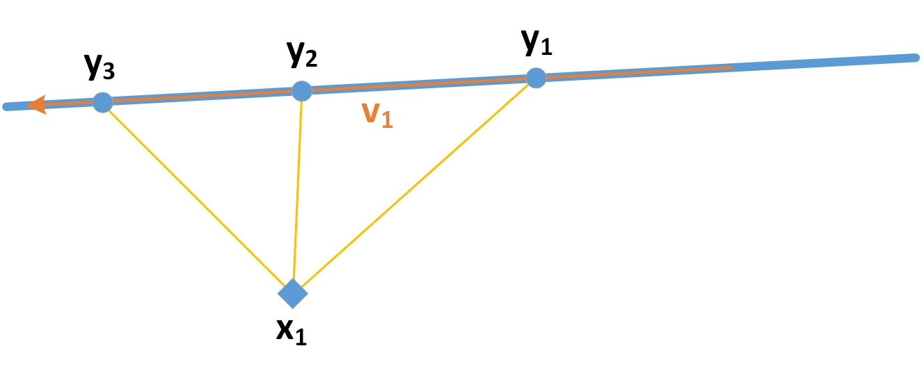
Figure 1: Linear motion of points, observed by $x_{1}$.

This concept of an individually moving point, besides the independent coordinate system of the line with points $y_{i}$ itself, allows to introduce a velocity from the viewpoint and in the coordinate system of the observer which may be synchronized easily assuming the Newtonian picture with overall or absolute time throughout the complete description of the system.

If in addition, we allow for the observer to move freely, the trajectory of the observer at $x_{1}$ is a line, too. Note, that we may immediately symmetrize this picture by switching the rôles of point and observer, or formally switching the coordinate system as known from classical physics and special relativity.

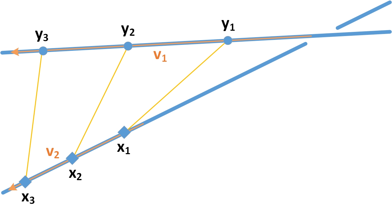
Figure 2: Linear motion of points, observed by a linearly moving observer $x_{i}$.

If we now proceed as before by connecting points on the two lines (see Figure 2), it is the notion and additional interpretation of ’moving points’, where adjacently observed velocities $v_{i}$ connect ’times’ to causality in the respective (local) coordinate systems by ordering the points and their related description(s) of physics. On the one hand, as such we can introduce and use individual (point) coordinate systems or apply the typical reasoning of special relativity in terms of point (or four-vector) coordinates. On the other hand, the picture of projective and especially line geometry offers two well-established frameworks to describe such a setup much better by taking into account the individual planar geometries of the two line pencils and the overall picture of a ruled surface or a line Congruence (see Figure 2). In one approach, we may interpret each of the lines as a special linear Complex, and identify common lines within the superset of lines intersecting each of the two lines. There is, however, a second possibility in that both lines do not belong to the same linear Complex. Then, we may construct a regular linear Complex $a_{\mu\nu}$ by $a_{\mu\nu}=\lambda p_{\mu\nu}+\rho q_{\mu\nu}$ where $p_{\mu\nu}$ and $q_{\mu\nu}$ are the line coordinates of two skew lines $p$ and $q$.

Whereas we’ve given already some arguments and references on line geometry and Complexe to justify the deep rôle of Congruences, we also want to mention a background paper with respect to the Figures 1 and 2. Whereas nowadays people tend to discuss ’time reversal’, often in the context of space symmetries and special relativity, and mostly by means of Euclidean coordinate interpretations, it seems helpful to recall Klein’s paper klein:1872c which reviews the (even at that time historical) discussions and interpretations of complex numbers and measures within the context of line geometry. Referring for details to Klein’s paper, he connects two complex points (a point and its conjugate point) by a real line. So the two points can be seen as base points in order to define an involution on the real line. Being quadratic, in order to resolve for the (complex) point, one has to define an orientation of the line which has been proposed by von Staudt. Klein resolves this apparently ’artificial definition’ by referring to projective definition of measure (i.e. the Cayley-Klein measure (’metric’)) on the line using the two points as base points. So the sign given by the definition of the measure distinguishes both sets of base points, or the individual complex point, respectively. Using point pairs, he obtains von Staudt’s interpretation, and thus the orientation of the line. The final identification with the quadratic covariant $\Delta$ allows to represent a complex point by three arbitrary points of a certain order.

A second major consideration regarding ’observers’ is to tag one plane in space as an ’absolute plane’ and to shift one point of the coordinate tetrahedron (or one of the two observers above) to this absolute plane, i.e. to $\infty$. We thus obtain affine geometry, and by an additional assumption with respect to a circle in the absolute plane (the ’infinite circle’) Euclidean coordinates and parallelism. If we associate this description with ’classical physics’ (where affine transformations leave the absolute plane invariant), then we may ask which physics is related to the scenario in Figure 2 when both observers are close to each other (and both are far from the absolute plane, or if no ’absolute plane’ is present at all!). By analogy to a common experimental setup, we suggest to identify this physical picture to quantum theory where the ’observer’ and ’point’ are both part of the interaction/the ’process’. Why? Thinking of electron scattering on a target, $e(\cdot,\cdot)e^{\prime}$, as related experimental setup, we have two major possibilities to let the first vertex $e\longrightarrow e\gamma$ happen. If the distance of this first vertex is far from the target, people usually assume outgoing real photons $\gamma$ and calculate the ’tagged photons’ by standard relativistic kinematics and by measuring both electrons. So the second vertex of the reaction is going to happen ’far away’ with (idealized) real photons at the target. If we shift, however, the first vertex into the target by scattering the electrons directly by or within the target, we have to work with ’virtual photons’, and the overall kinematics is governed by the effective descriptions of $e(\mathrm{target},X)e^{\prime}$-processes with all known phenomenological implications.

The difference of both pictures is that we move ’the observer’ (represented by the first vertex $e\longrightarrow e\gamma$ ’to generate’ the observation by a photon) close to the target of the observation, and we want to have only one unified framework to describe the process and the involved reps. That’s why we want to use projective geometry to shift both vertices freely, and we have to adopt our description of physics appropriately. In order to work with overall valid reps, we thus emphasize line and Complex geometry in terms of homogeneous coordinates of 3-dim space.

Besides being still free to use individual coordinate systems related to each line (e.g. in associating the six line coordinates to the sides/lines of a (fundamental) tetrahedron), we can use in addition the two lines of the trajectories (moving observer and moving point) as opposite sides of a (third) tetrahedron and introduce ’overall’ coordinates (with an additional unit point and (if necessary) absolute elements or by associating the framework of tetrahedral Complexe) in order to establish a common description/coordinatization of both systems. So we’ll have to work out the algebraic relations of the respective six line coordinates of the two individual line identifications used to describe the two individual coordinate identifications versus using a common (fundamental) tetrahedron related to a parametrization by relative velocity and an abstract overall time which will result in identifying point sets of line incidences and harmonic ratios and relating them while respecting (some or all) properties of projective transformations. This reminds correlating one-particle rep descriptions in quantum field theory (QFT) in order to find common and comparable physical behaviour like in Smilga’s nice work (see smilga:2011 or dahm:QTS7 ). Moreover, we can ’collect’ all the lines connecting the two trajectories (at different (individual) times and as such space points, of course) and describe them via line incidences of both lines, or more general in a first step by singular Complexe, ray systems (see footnote before) and by appropriate Congruences. This can be done not only in Euclidean geometry but the framework of line geometry (because imbedded in projective geometry) is available also for all types of non-Euclidean geometries. The physical picture of such a description becomes transparent and clear if in mind we associate a ’light’ source to both the moving point and the observer, and if we think in terms of rays being emitted by the point and by the observer, respectively. Nonlinear movements can then be described by e.g. higher order (or higher class) curves and surfaces, and projective geometry provides dimension formulas and a lot of further useful tools. Thus, the ’physics’ or dynamics is directly related to the geometry of the respective curves and/or trajectories. As mentioned above, the breakdown to (squares of) line elements $\mathrm{d}s^{2}$ is possible in various ways and respecting/representing various geometries and associated symmetry groups.

III Physics and Complexe – a Programmatic Approach

Having gathered and summarized so far some geometrical aspects as well as few Ansätze in physics throughout the last section II, the different ’types’ of line sets termed ’Complex’, ’Congruence’ and ’Configuration’ by Plücker plueckerNG:1868 need some context, especially in that this geometry according to our opinion should be re-invoked for analytical use. In section II, we have summarized few aspects from electromagnetism and (special) relativity, and their relation to linear Complexe, which we want to discuss in more detail in upcoming publications. Plücker himself has given a detailed account in pluecker:1865a on how to use Complexe, he has had suggested Dynamen, and how to summarize the description of force systems of mechanics pluecker:1865b . This concept has had found a certain closure and completion from the viewpoint of classical geometry by Study’s discussion of different geometries, Dynamen and of Somen study:1903 .

Having seen the importance and usability of these concepts, which seem to be directly and strongly connected to physical terminology and geometrical descriptions, we feel the need to approach this notion more programmatically, and as such we want to propose and later on follow an identification scheme based on line Complexe which we feel suited to unify mechanics and various features of electrodynamics and special relativity geometrically. Based on pluecker:1838 and Plücker’s considerations in optics, we have discussed in section I.6 an established geometric possibility to relate lines or Complexe to sphere geometry, which we assume suitable to investigate quantum properties, too. Thus, we feel prompted to propose the following Complex-based ordering scheme or ’program’ in order to relate structures and content as far as we understand these relations now, starting by quadratic Complexe.

III.1 Remarks on Geometry

With respect to the general idea, and in order ’to resolve’ a natural ’chicken-and-egg’ problem right at the beginning, it is necessary to recall that – starting from projective geometry of 3-dim space – points and planes are understood as 3-dim ’objects’, although represented by 4-dim homogeneous coordinates $x_{\alpha}$ and $u_{\alpha}$ in $P^{3}$, and although people ’feel’ a close relation to 3-dim space of physical observations. If plane ’objects’ are included, a transfer principle (’duality’) allows to symmetrize this picture as has been established already long ago by classical projective geometry (see e.g. enriques:1903 and references). The apparatus of this geometrical approach relies on intersections and incidences being preserved by projective transformations, which is close to physical observation like e.g. in the case of point-plane incidence $x_{\alpha}u_{\alpha}=0$.

However, with respect to using line geometry, concepts are different. Plücker has shown already in his early text books (see references in plueckerNG:1868 ) that line space is 4-dimensional, i.e. each line can be represented by 4 parameters. Being derived only from Euclidean geometry, because equations in these four parameters do not preserve grade under projective transformations, Plücker in addition has introduced the determinant $\eta$ of his original four line coordinates to establish covariance of the five inhomogeneous parameters, thus preserving grade of the equations with respect to projective transformations. This concept may be embedded in $P^{5}$ using six parameters (or line coordinates) as given in eq. (3) with respect to their construction by point coordinates of $P^{3}$. The Plücker condition used above is necessary ’to reduce’ 4-dim line geometry to 3-dim geometry of real space, however, we may still use the established framework of projective geometry with respect to incidences, intersections and transformations. In other words, although we use lines and ’generate’ points by intersection of lines and span planes by joints of two incident lines, we are still consistent with projective geometry, and we are moving on the solid ground of Klein’s ’Erlanger Programm’.

Because this concept introduces a ’chicken-and-egg’ problem with respect to $P^{3}$ as the space of point-/plane-reps, and $P^{5}$ as the space of Complex reps, we have to find equivalence relations and transfer principles. This may be established by eq. (3) if we introduce the Plücker condition, or the Plücker-Klein quadric in $P^{5}$, respectively. This establishes a quadratic constraint in $P^{5}$ which has to be fulfilled for points in $P^{5}$ on the quadric in order to correspond to lines in $P^{3}$. So in $P^{3}$, we have to take care of quadratic algebras and involutions additionally! Moreover, the points of $P^{5}$ are thus separated by the quadric, and accordingly, we have to distinguish regular and singular (’special’) Complexe. Because the relation to linear point coordinates relies on the definition of the fundamental tetrahedron in $P^{3}$, we have to compare to lines in $P^{3}$, i.e.  points in $P^{5}$ on the Plücker-Klein quadric.

So, the starting point here is not $P^{5}$, but while representing the objects of $P^{5}$ in $P^{3}$, for us it is natural to discuss quadratic and linear Complexe in $P^{3}$ with respect to the very coordinate definition of $P^{3}$ in terms of the fundamental tetrahedron.

III.2 Tetrahedral Complex

To work with line reps and Complexe in $P^{3}$, we thus depart from the tetrahedral Complex and it’s property, that the Complex lines intersect a (fundamental) tetrahedron by constant harmonic ratio for all lines of the Complex . Besides self-duality of the Complex, we thus benefit at the same time from invariance properties of projective (point) transformations when working with linear coordinates of points and planes, and of correlations (or duality, or general transfer principles).

So this picture allows to relate various well-known descriptions and interpretations as soon as we have developed the line/Complex part on a parallel footing to classical affine and projective geometry in terms of points, planes and their various generated, higher-order objects. So besides analytical expressions, we feel the need to sketch briefly an accompanying ’program’ in section III.4 which we want to execute step by step in order not to get lost in a plethora of analytical/geometrical details.

III.3 Overview Complexe

We’ve mentioned various examples of linear and quadratic Complexe already above, referring to some physical associations and relations.

As such, and with respect to known physical applications, here we choose quadratic Complexe as general origin of our discussion, and try to drill down to linear Complexe and to the standard geometry of 3-space, usually described in (metric or affine) point coordinates. Note, that in the spirit of the old geometers, we do not emphasize complex numbers and Riemannian geometry, but we see complex (and hypercomplex numbers) for a while as additional symbols to represent geometry appropriately on real spaces according to the need to linearize the square ’-1’, e.g. to treat non-intersecting situations or the closure of the projective line which (formally) relates it to circles.

III.4 Quadratic Complexe

We’ve commented on the central rôle of the tetrahedral Complex and its relation to the fundamental coordinate tetrahedron above. We may add that for special tetrahedra (having e.g. their four vertices on a sphere), we can discuss polar relationships and include the center of the sphere as unit point. This simplifies the coordinate description of spheres in that we may omit weights and end with a sum of squared coordinates. The tetrahedron is related to tetrahedral Complexes because all lines in (3-dim) space constitute fixed harmonic ratios with respect to the points of intersecting the four tetrahedral planes. So we may use these ratios to group lines in space.

This suggest a certain program to follow:

1. As mentioned in section III.2, considering ’Würfe’ vonStaudt:1856 and their invariance properties with respect to projective transformations, we have found a base point or departure of invariance discussions because projective transformations (i.e. the basic tool of Klein’s ’Erlanger Programm’) can be directly related to invariance groups. Here, we can attach the discussion of discrete and continuous/Lie groups, and we can also attach the construction scheme of projective geometry, departing from 1^st order/class objects, and constructing higher order/class objects while preserving invariance of incidences. Typical questions comprise coordinate systems and calculus with respect to the different scenarios/objects.

2. If we depart from projective geometry and, in a next step, fix additional geometrical structures as ’invariants’ (or ’absolute’) objects, on the one hand, we follow precisely Klein’s ’Erlanger Programm’. On the other hand, we have already discussed above the case of an absolute plane which leads to ’affine’ coordinates, and Klein’s introduction of the metric in the Euclidean case as an ’absolute circle’ in the ’absolute plane’. Due to several reasons, we want to extend this approach as we have argued already in section I.6. There, we have associated the typical ’metric’ in Minkowski space with an invariance of a quadratic Complex, and we’ll have to investigate more consequences of parameter choices of the quadratic Complex as well as further possibilities of different absolute elements by means of quadratic or linear Complexe. In section III.5, we’ll discuss also a related change in the very coordinate definition which yields interesting results with respect to relativity and typical quantum formulations.

3. Having fixed a $2^{nd}$ order surface in $P^{3}$, we may benefit from the Cayley-Klein approach to metrics, i.e. the metric is not given by god (or a scientist), but it is strictly related to a geometrical setup and some of the assumptions (see eq. (8) or (9)) above. Then, of course, we may fall back to purely analytical discussions (having to take care about the coordinates, however), and proceed with point and appropriate differential geometry. From the viewpoint of line geometry which we want to pursue, it is however helpful to investigate the (quadratic) tangential Complex plueckerNG:1868 and its properties. Besides the relations between such types of Complexe and $2^{nd}$ order surfaces, we want to recall also the normals of confocal surfaces which constitute a $2^{nd}$ order cone plueckerNG:1868 , and for our own considerations later on, we want to recall the generation of $2^{nd}$ order surfaces by lines. So with respect to tangential considerations (where we nowadays discuss dynamics and Lie theory), it is obvious that we may use as well an approach by generating lines and polar systems in order to cover the tangential discussion not only in this singular point of the tangent space, but line geometry and Complexe allow global calculations and definite, and controllable, reductions schemes to the tangential case.

4. So one of the last steps which are needed to complete such a program is the reduction of quadratic to linear Complexe, or in other words, to find consistent analytic reps in point/plane as well as in line space to represent square roots. So whereas this concept is already well-known from Dirac’s approach to quantum theory to resolve the Minkowski ’norm’ into two conjugate linear reps, however, to our opinion the 6-dim line (and momentum) reps are much better suited, because forces and force systems have to be described by Complexe (see pluecker:1865b , plueckerNG:1868 and references). As such both sources, Plücker plueckerNG:1868 , and Klein’s reprise klein:1872b , are relevant from the physical viewpoint in that Klein (klein:1872b , §2) with respect to an arbitrary Complex line and the quadric $\Omega$ in $P^{5}$ discusses the ambiguity of the related linear tangential Complex, and he points out the relevance of a special linear Complex as well as a special Congruence. Mathematically, we may use Clebsch’s discussion clebsch:1869 to proceed to Complex calculus, and quaternary forms and invariants. We want to apply this discussion to matter fields, and to photons coupling to matter, as well as the typical Lagrangean descriptions of QED and gauge fields. Due to the identification of the photon with a special linear Complex in section II.1, we have to investigate the role of linear special Complexe as well as the role of regular Complexe in both of the geometrical contexts of $P^{3}$ and $P^{5}$.

5. So last not least, we have to focus this ’program’ to usual Hamiltonian or Lagrangean formulations in order to finally discuss equations of motion and conserved quantities. In other words, the connection can be found by the usual invariant theory of Hamiltonian/Lagrangean formalisms and its relation to quaternary invariant theory of Complexe in terms of coordinates in $P^{3}$, or even directly of forms and invariant theory in $P^{5}$. The variation with respect to (general or restricted) projective transformations can be formulated in terms of $\delta\mathcal{L}=0$, if the Lagrangean can be expressed in irreps of either point/plane combinations and forms in $P^{3}$, or 6-dim reps and invariants of lines or linear Complexe. So we’ll have to investigate invariants of QED type $F_{\mu\nu}F^{\mu\nu}$ or Yang-Mills type $F^{a}_{\mu\nu}F^{a\,\mu\nu}$, $1\leq a\leq 3$, in the Lagrangean framework, and we can compare to Klein’s discussion of six linear fundamental Complexe which span $P^{5}$. Besides the identification of the individual geometrical objects, the major problem will be to find the correct coordinate reps with respect to the symmetry groups SO($n$,$m$), $0\leq n,m\leq 6$, where $n+m=6$, and the groups SU($n$,$m$), $0\leq n,m\leq 4$, where $n+m=4$, and their respective physical interpretations.

III.5 ’The Metric’ Revisited

In order to gain more control on coordinates and especially the metric as discussed in section I.4, it is noteworthy to recall some old geometry. Usual geometrical and physical considerations often assume – at least intrinsically – rectangular coordinates and differentiability like $\mathrm{d}x_{i}$ (or their two relevant ratios $p$ and $q$, respectively) when working with 3-dim space and describing physics. In order to gain more control, we do not start from Cartesian descriptions or Weyl’s axiomatization of ’affine geometry’, but it seems helpful to recall that the ’extension’ of Cartesian/Euclidean coordinates $x^{\prime}_{i}$ to affine coordinates contains the assumptions cited above, i.e. the additional assumption of an invariant plane ’at infinity’, and a polar system, the ’absolute circle’ in this ’absolute plane’, to handle parallelism and orthogonality. Please remember during all our discussion, that the concept of ’absolute’ or ’ideal’ elements historically has been introduced to unify the analytical description of geometry, e.g. of (planar) lines intersecting always in one planar point!

Analytically, in usual terms one introduces four ’homogeneous coordinates’ $x_{\alpha}$ of 3-dim space, $0\leq\alpha\leq 3$, by

$$x^{\prime}_{i}=\frac{x_{i}}{x_{0}}\,,1\leq i\leq 3\,,$$ (10)

or from a more general and complete view

$$x^{\prime}_{\alpha}=\frac{x_{\alpha}}{x_{0}}\,\sim\,\left(x^{\prime}_{i},1\right)\,,0\leq\alpha\leq 3\,,$$ (11)

thus giving rise to the usual ’reduction scheme’ to the primed Euclidean ’point’ coordinates $x^{\prime}_{i}$, used e.g. in eq. (7). Here, $x_{0}=0$ describes the coordinatization of the ’absolute plane’ by homogeneous coordinates, and the coordinates $x^{\prime}_{i}$ as quotients of homogeneous coordinates are associated with the three Euclidean coordinates. So intrinsically (although people usually suppress the fourth coordinate $\sim 1$), the Euclidean coordinates (11) remember their relation to the absolute plane of the affine picture. Details can be found e.g. in enriques:1903 . So the geometrical and synthetical identification of the ’absolute plane’ in projective geometry finds its analytical counterpart in an intrinsic divergence of the Euclidean coordinates for $\lim_{x_{0}\to 0}$. Taking this limit $\lim_{x_{0}\to 0}$ on a second order sphere $S=\sum_{\alpha}x_{\alpha}^{2}=0$, $S$ yields $\sum_{i}x_{i}^{2}=0$, i.e. we ’find’ a circle in the ’absolute plane’ $x_{0}=0$ constituted by the three remaining homogeneous coordinates $x_{i}$ which thus can serve as general planar coordinates.

Now, this coordinate definition, and the ’affine’ notion, both appear to be consistent as long as we regard transformations which leave this plane invariant, i.e. transformations of points and planes which do not alter the $x_{0}$-coordinate, as is usually assumed to be a property of ’affine’ transformations.

However, care has to be taken already with Lorentz transformations. While in usual ’Euclidean’ notation, the plane normal to the velocity is left invariant by Lorentz transformations, the coordinates of the velocity direction and ’time’ mix. On the other hand, everybody ’knows’ that (special) Lorentz transformations leave ’the norm’ $x_{0}^{2}-\vec{x}^{\,2}$ invariant which may be interpreted as a cone (according to rank and signature of the spatial form), or in general as a $2^{nd}$ order surface.

Now, in order ’to produce’ geometrically the same behaviour of infinite coordinates $x^{\prime}_{i}$ like in the affine case (11) for $x_{0}\to 0$, we necessarily have to switch to a more general and ’more symmetrical’ coordinate definition $y^{\prime}_{\alpha}$ in 3-dim space,

$$y^{\prime}_{\alpha}=\frac{x_{\alpha}}{\sqrt{f(x_{\alpha})}}\,,0\leq\alpha\leq 3\,,\quad f(x_{\alpha})=x_{0}^{2}-\vec{x}^{\,2}\,.$$ (12)

So with respect to this ’new’ set of coordinates $y^{\prime}_{\alpha}$, we can check their behaviour with respect to homogeneity (i.e. $x_{\alpha}\to\lambda x_{\alpha},\lambda\in\mathbb{R}$). We obtain $f(\lambda x_{\alpha})=\lambda^{2}f(x_{\alpha})$, or $\sqrt{f(\lambda x_{\alpha})}=\pm\lambda\sqrt{f(x_{\alpha})}$, so the linear coordinate definition $y^{\prime}_{\alpha}$ in (12) as a quotient is independent of $\lambda$, and thus they show the same behaviour as the ’original’ Euclidean coordinates $x^{\prime}_{\alpha}$ in eq. (11). If we now build the expression ${y^{\prime}_{0}}^{2}-{y^{\prime}_{i}}^{2}$ while using eq. (12), this expression in the four new coordinates $y^{\prime}_{\alpha}$ yields

$${y^{\prime}_{0}}^{2}-{y^{\prime}_{i}}^{2}=\frac{x_{\alpha}x^{\alpha}}{f(x_{\alpha})}\equiv\frac{f(x_{\alpha})}{f(x_{\alpha})}=1\,,$$ (13)

and it is even independent of the (original) homogeneous coordinates $x_{\alpha}$ of 3-dim space at all as long as $x_{\alpha}$ in eq. (12) is acted upon with SO(3,1) transformations, i.e. the expression $x_{\alpha}g^{\alpha\beta}x_{\beta}$ is preserved. We’ll have to discuss parallels to the absolute circle $\sum_{i}x_{i}^{2}=0$ from above elsewhere. Using the first equality in (13), it is obvious that this relation is independent with respect to $x_{\alpha}\to\lambda x_{\alpha}$, so the homogeneity of the four coordinates $x_{\alpha}$ doesn’t influence the quadric in the new coordinates $y^{\prime}_{\alpha}$, however, the linear coordinates individually (and symmetrically) tend to $\infty$ as the original quadric approaches the ’light cone’. The most important difference between $x^{\prime}_{\alpha}$ in eq. (11) and $y^{\prime}_{\alpha}$ in eq. (12), however, is the suitability to define valid coordinates as long as we transform the linear reps $x_{\alpha}$ by all SO(1,3) transformations. Note, that this is in general not the case for ’affine coordinates’ according to eq. (11) due to $x_{0}$ appearing linearly in the quotient.

With this ’new’ coordinate definition $y^{\prime}_{i}$, we take care of the symmetry that the full group of special relativity defines appropriate limits with respect to one and the same ’absolute element’ $f(x_{\alpha})=0$, the invariant sphere, and not an non-invariant plane $x_{0}=0$. This has, of course, enormous consequences which we’ll have to discuss elsewhere. For now, it is sufficient to discuss the special case of affine geometry by the equation

$$\sqrt{f(x_{\alpha})}=\sqrt{x_{0}^{2}-\vec{x}^{\,2}}=\sqrt{x_{0}^{2}}\sqrt{1-\frac{\vec{x}^{\,2}}{x_{0}^{2}}}=x_{0}\sqrt{1-\frac{\vec{x}^{\,2}}{x_{0}^{2}}}$$

So the ’new’ set of coordinates $y^{\prime}_{i}$ in eq. (12) comprises the standard Euclidean coordinates up to a well-known factor,

$$y^{\prime}_{i}=\frac{x_{i}}{x_{0}\sqrt{1-\frac{\vec{x}^{\,2}}{x_{0}^{2}}}}=\frac{x_{i}}{x_{0}}\frac{1}{\sqrt{1-\frac{\vec{x}^{\,2}}{x_{0}^{2}}}}=x^{\prime}_{i}\frac{1}{\sqrt{1-\frac{\vec{x}^{\,2}}{x_{0}^{2}}}}\,,$$ (14)

where we recover the old Euclidean, ’affinely constructed’ coordinates $x^{\prime}_{i}$ of eq. (10). If we consider only special relativity, we may assume the typical identification of a light cone (or light ’sphere’) by $x_{0}=ct$, and while considering uniform linear motion in the coordinate projections $x_{i}$ by introducing appropriate velocity projections $x_{i}=v_{i}t$ per same ’overall’ time interval $t$. So the fraction most right in eq. (14) above is based on the ratio of velocities, and equals to $\gamma=\frac{1}{\sqrt{1-\beta^{2}}}$, the Lorentz factor. So eq. (14) reads as $y^{\prime}_{i}=\gamma\,x^{\prime}_{i}$. The denominator can be decomposed further by $\sqrt{1-\beta^{2}}=\sqrt{1+\beta}\sqrt{1-\beta}$, or if we switch back to homogeneous coordinates, according to $\sqrt{x_{0}^{2}-\vec{x}^{\,2}}=\sqrt{x_{0}+\|\vec{x}\|}\sqrt{x_{0}-\|\vec{x}\|}$ which both suggest to investigate higher order/rational curves and elliptic functions (or even integer squares, or triangular numbers) later on.

IV Outlook

Having in mind how we have associated (physical) light with ’light cones’ above, we have additional possibilities on a linear representation level to generalize lines (i.e. singular Complexe) to general linear (and higher degree) Complexe and, moreover, we can investigate their relation to ’massive’ reps ’on’ and ’off’ the mass shell. So what is open today is an a priori explanation of the Hamiltonian structure (and as such the energy) of being quadratic in line coordinates. So the generalization (and also our ongoing program if we think on how to approach general relativity) is twofold: We can extend the use and application of Complexe and Complex geometry, and we can investigate their various constraints with respective mappings to physics.

Because differential geometry (by using forms linearly) a priori reflects only (polar) parts of line reps and affine behaviour, we are convinced to find additional energy-momentum contributions to $T^{\mu\nu}$ (in four-vector notation) by simply taking elements of line or Complex reps (e.g. moments) into account or even more sophisticated mechanisms of line or Complex geometry. Moreover, we see differential forms, Pfaffian equations (one-forms) and Lie theory as subsidiary concepts of line geometry only in their respective (inhomogeneous) ’time’ dependent limits. Using line geometry, the inclusion of observers is a priori guaranteed by the formalism, i.e. we do not have ’observer-free’ physics as nowadays usual, and there is no need to speculate on ’non-localities’. Last not least, with respect to dimensions of transformation groups and concerning reality conditions so far, we want to mention the possibility that in choosing a ’correct’ set of coordinate reps we may associate the 15-dim resp. 16-dim transformation groups with projective transformations mapping (linear) Complexe to Complexe and the 10-dim subgroup mapping null lines to null lines. However, that’s an open issue right now and has to be proven formally which we want to pursue by executing the ’program’ sketched in section III.4.

At the time of writing, we see various still ’competing’ possibilities to work with 5-dim $p$ (or $\exp p$) and identify the space physically (better: dynamically!), and we feel the need also to discuss the double 15-dim (automorphic) collineations of $M_{4}^{2}$ with respect to physics and real/complex descriptions much deeper in those contexts. This is especially interesting when starting from Hamiltonian formalism while using/identifying line coordinates and assuming the quadratic structure as originating from $M_{4}^{2}$ as the fundamental form (see klein:1872a ). We have given above already one application of polarity, however, we have to investigate the physical consequences in much more detail. We have mentioned as well tangential Complexe and Congruences which we have to arrange versus the current concept of affine connections (see e.g. klein:1872b ).

Another open problem is the identification of Complex-related numbers and/or constants versus reps and rep dimensions in the Lie group/algebra related approach, i.e. there are 15 constants mapping the Plücker constraint linearly onto itself, there exist polar systems depending on 20 constants (and series thereof as well) which map (arbitrary) lines to linear Complexe and vice versa, etc.

We are convinced dahm:QTS7 that various low-dimensional Lie groups and algebras, especially su(2)$\oplus$u(1), occuring in various applications of QFT are artefacts of certain aspects of line (and projective) geometry of $\mathbb{R}^{3}$ which emerge by taking and generalizing certain analytic and algebraic aspects of line (and Complex) reps only in terms of individual ’calculuses’ and ’rules’. As such we see Plücker’s $M_{4}^{2}$ and the twofold 15-dim automorphisms in a central rôle, governed however by the rules of projective geometry. In this context, there are lots of further deep geometrical connections to other topics like Kummer’s surface, Darboux’s 5-dim reps of confocal cyclids, Pasch’s sphere Complexe and their geometry or to rep dimensions occuring both in line/Complex geometry and physical/QFT rep identifications which we have to work on.

IV.1 Remarks

Having been asked to contribute to a topical collection of AACA, in memoriam of Waldyr Rodrigues, for me it is a real honour to contribute, and to dedicate this work to such a great mathematical physicist. Having been a great scientist who left a lasting personal impression, and a real maker with respect to his university environment and to the AACA community, he is and will be very much missed!

With respect to the circumstances and the focus on relativity and field theory, I’ve decided to contribute the original, extended and so far unpublished version of the ICCA 10-contribution in Tartu, Estonia, 2014, where our last personal meeting took place. The content presents geometrical aspects of field theory, electromagnetism and relativity from a projective point of view, and tries to fit to Waldyr’s work and interest in those topics.

Since then, we’ve published several parts of the series related to aspects and steps discussed in section III, and especially subsection III.4. So while executing this program, we have included Cartan’s spinor calculus, based on Study’s work, by relating it to Lie’s transfer of line and Complex geometry to spheres dahm:2017a . Moreover, we have shown dahm:2017b so far that Minkowski’s 4-vector calculus basically relates to (linear) Complex and projective geometry. In both cases, work on further identifications and calculations is ongoing.

Appendix A A Projective Setup

As an interesting and self-evident scenario we want to discuss the scenario depicted in Figure 3 with respect to physical aspects.

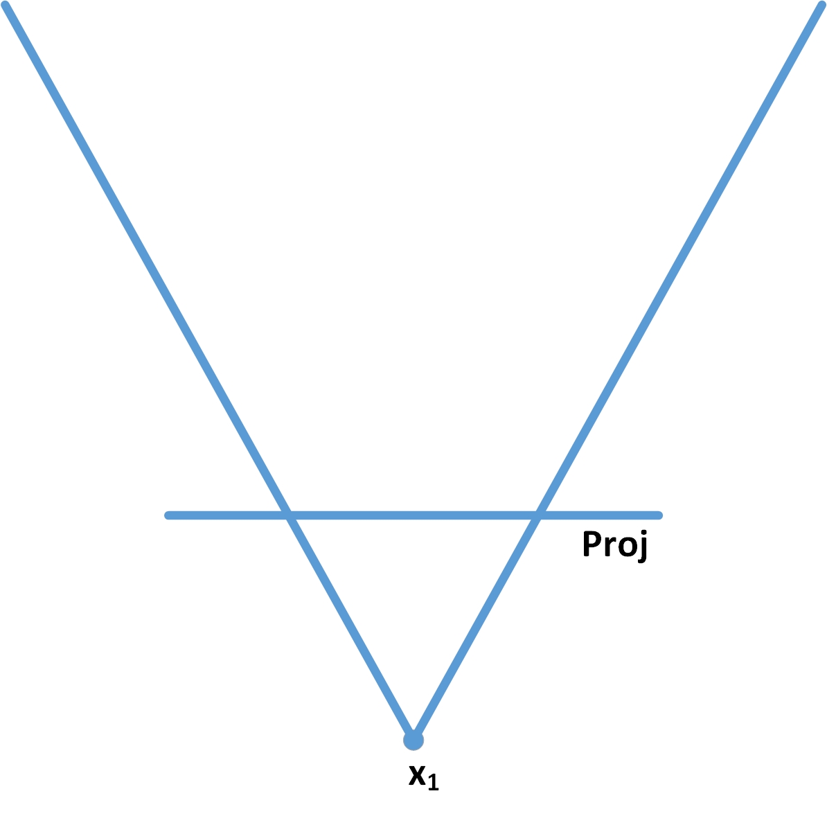
Figure 3: Geometrical setup of observer and observation.

In this setup, we assume that the observer located at $x_{1}$ can observe a (planar) physical process only by means of a projection to the line ’Proj’, and the measurement of the projection on ’Proj’ takes place at equal time intervals $\Delta t$. So the individual time values of the observations are associated to positions $x_{i}$ on ’Proj’, and we can also introduce the concept of velocities to quantify changes (or dynamics) with respect to different observations and the interval $\Delta t$ from the viewpoint of the observer.

The observer ’lives’ on one side of ’Proj’, the physical process takes place on the other side. For the sake of simplicity of the description, we assume moreover, that the observer can watch the process only within the view limited by the two lines in Figure 3.

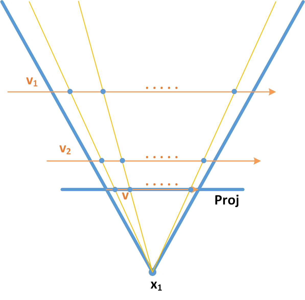
Figure 4: Observer and observed parallel/linear velocities.

Now, if a point moves with slowconstant velocity $\vec{v}$ infinitesimally close and parallel to the projection line ’Proj’ (see Figure 4), we can determine its velocity by, e.g., measuring its location (more precisely, the location of the projection on the line ’Proj’) at certain times and calculating the velocity classically. If we draw virtual projection lines from the observer to the observed points on the projection line (where we measure space versus time), we obtain first of all a pencil of lines with center $x_{1}$. The description of the velocity will correspond in this case to the real physical velocity of the point.

However, if there are further movements of points parallel to the original process described by $\vec{v}$ and with constant velocities $v_{1}$ and $v_{2}$ like in Figure 4, they cannot be distinguished from the first process as long as the velocities are higher and meet at the same time of measurement the projection lines (of our observation/our observer). It is obvious that in order to establish such an identification, the velocities have to increase dependent on the distance from the projection line/the observer (which, however, is beyond the scope the observer at $x_{1}$ can detect or know, having only data from measurements on the projection line ’Proj’. So the absolute value $\|\vec{v}\|$ is a lower bound on the velocity, and the observer – without additional information – is not able to determine the exact value of the ’real’/physical velocity of the point.

In other words, already in this simple setup, we find equivalence classes of velocities as a function of distance (or space), and in addition, we find a lower bound on $\|\vec{v}\|$ dependent on the position (or distance) of the projection line from the observer. These uncertainties are already apparent in classical physics, and the only possibility to resolve this scenario and perform complete and correct analytical calculations is to gain additional knowledge on the setup, here on the additional distance information in order to determine the exact $y$-coordinate of the moving point if we assign $x$ to the projection line ’Proj’.

So introducing nothing but the projection process yields, by means of very basic projective geometry, obviously some features known from physics usually attributed to other contexts and pictures.

Nevertheless, we have further possibilities to extend this simple geometrical setup.

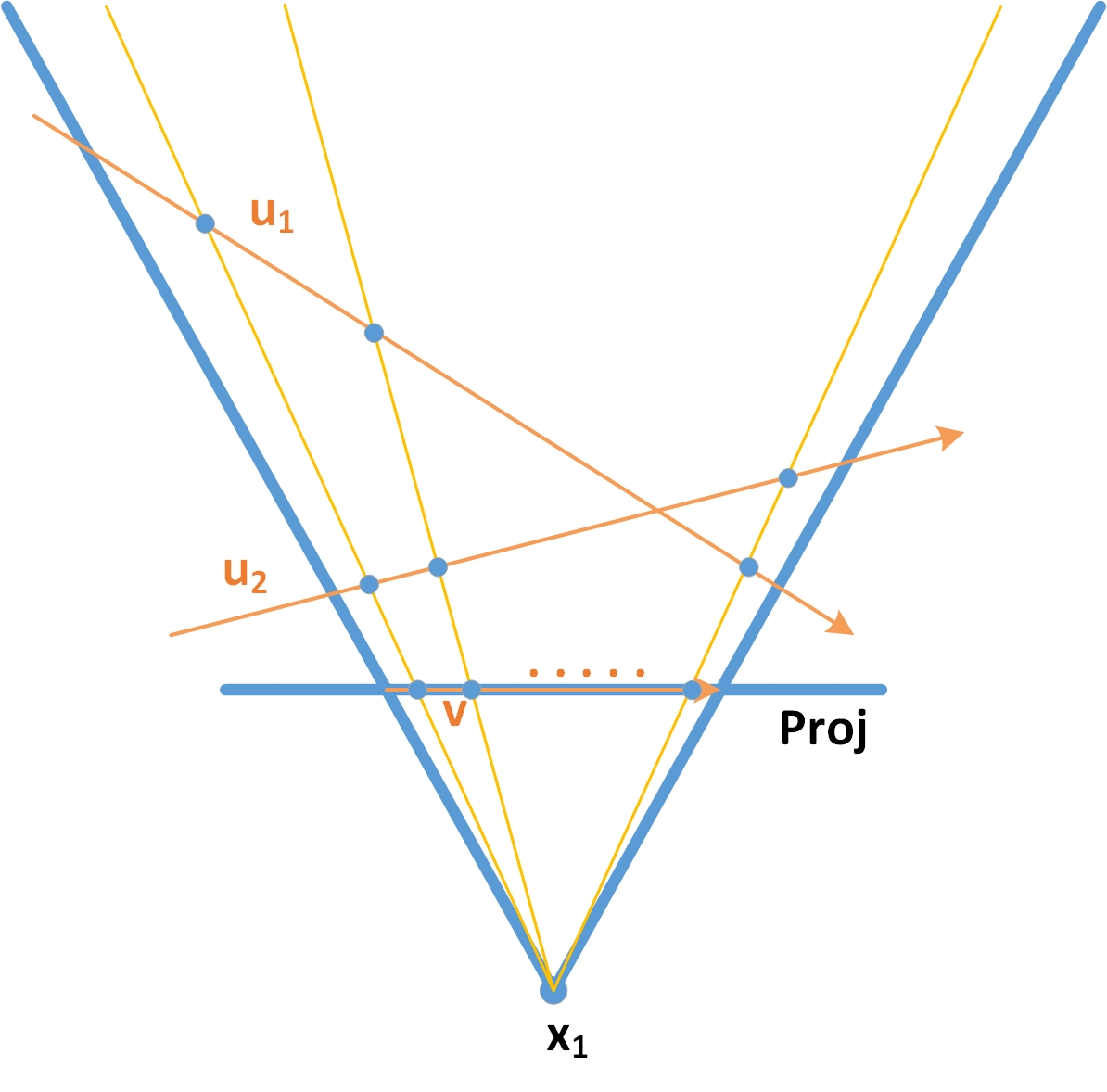
Figure 5: Observer and non-parallel linear velocities.

If as a next enhancement, we allow for non-parallel (but still linear) motion in the plane (see Figure 5), the description still holds, however, we have to consider this change with respect to velocities. Not only does the distance of the moving point, emerging between two points of our measurement on ’Proj’, increase at larger distance from the observer/the projection line, it also depends on the angle between the line ’Proj’ and the direction of the linear velocity. This, however, has to be ’absorbed’ in an accelerated/decelerated motion of the real physical motion of the point if we require the projection to maintain its uniform velocity. In other words, non-parallel, but linear motion decelerates as the point approximates the projection line/the observer, and accelerates otherwise.

So there are two lessons to learn by this enhancement:

• For the ’real’/ physical motion, we have to give up uniform/constant motion in order to maintain the old picture of the observation on the projection ’Proj’, so that for the (virtual) point moving on the line ’Proj’ the distance between two points of measurement (i.e. the intersections of the motion and the projection lines) is the same at same time intervals. This enhances our (planar) velocity classes by accelerated motions.

• From the geometrical viewpoint of Euclidean geometry, it is now obvious, that we have to take care of intersections of possible lines $u_{1}$ and $u_{2}$, i.e. even in the Euclidean description, we have to consider a second pencil with center at the intersection of $u_{1}$ and $u_{2}$. This is no real problem, but it shows that we have to switch our simple Euclidean description to a geometrically more suitable description in terms of line pencils and their (projective) properties. We can then include the case of Figure fig:app1 by assuming the center of the pencil in Figure fig:app1 at $\infty$. In terms of coordinates, to achieve a unified description already in this simple setup, we have to give up Euclidean coordinates and switch to projective geometry.

Having reached this stage, there are two further possibilities to enhance our original scenario:

1. From the viewpoint of projective geometry, having two line pencils at hand, it is obvious to take possible projectively generated, higher order objects as well as general projective (planar) theorems on points and line intersections into account. As such, we can switch to conic sections, e.g. to non-linear motion like in Figure 6 for a quadratic parabola.

   

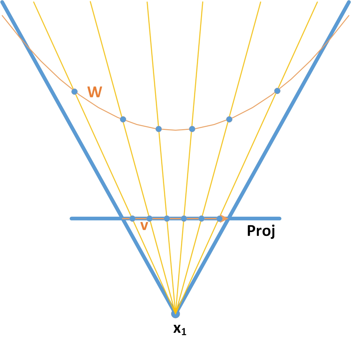
   Figure 6: Observer and non-linear velocities.

   The situation is similar to Figure 5, and we can discuss the mapping dependent on the various parameters of the parabola, or more generally, of second order planar curves. However, in addition to the parameters of the curve and the projection, we may also ask for the time deltas on the line ’Proj’. So also the quality of the measurement enters and influences the possibilities to determine the description of motion, i.e. for smaller $\Delta t$, we expect better possibilities to distinguish the various types of original motion.

   For uniform rotation, we’ll obtain trigonometric functions (as we’ll discuss in the examples of next appendix), so as long as the trigonometric function on ’Proj’ is close to the linearized version of the projection (within the quality limits of the measurement!), we find valid descriptions and we cannot distinguish (like e.g. in the case of a large radius of the rotation). So here, we have obviously entered a regime where care has to be taken with respect to physical claims, although the mathematical treatment is well-known e.g. in the context of contractions and Lie algebras (see gilmore:1974 , ch. 10).

2. Last not least, we may abolish the constraint on the observer to stay at $x_{1}$. Now, if the observer is allowed ’to enter’ the world behind the projection line ’Proj’, he will be able to gain more information (mostly due to his own motion), and we can apply the considerations given in section II.2.

   Moreover, from our reasoning above, it is obvious that the observation (if not obviously related to linear motion), due to the projective generation of the points of the time series, is related to planar pencils, and thus to conic sections as projective generation of two or more planar pencils with respect to their relative location. In other words, we expect to see special functions as solutions of the equations of motions related to such planar problems when including the observer.

We have discussed in section II.2 the case of ’real’ and ’virtual’ photons already. Like above, it is necessary to gain the freedom of moving the center of the pencils freely by means of projective geometry, even to an ’absolute plane’, or $\infty$, respectively.

Now, if instead of the parabola in Figure 6, we project a circular motion Figure 7 to ’Proj’, we are in the same situation. The information deficit due to the projective setup causes the original circular motion based on two variables $x$ and $y$ to be mapped onto one variable on the line ’Proj’, only.

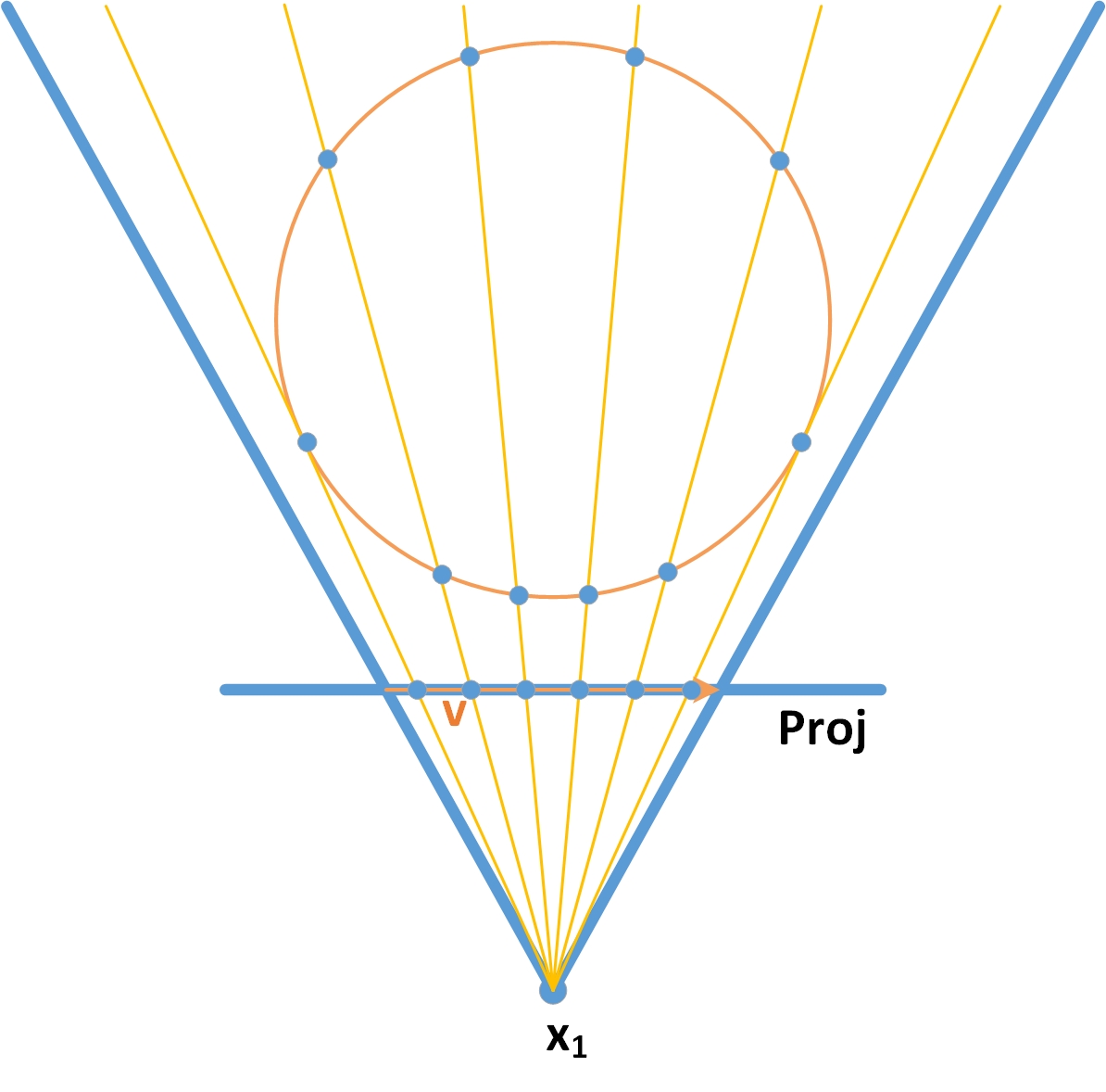
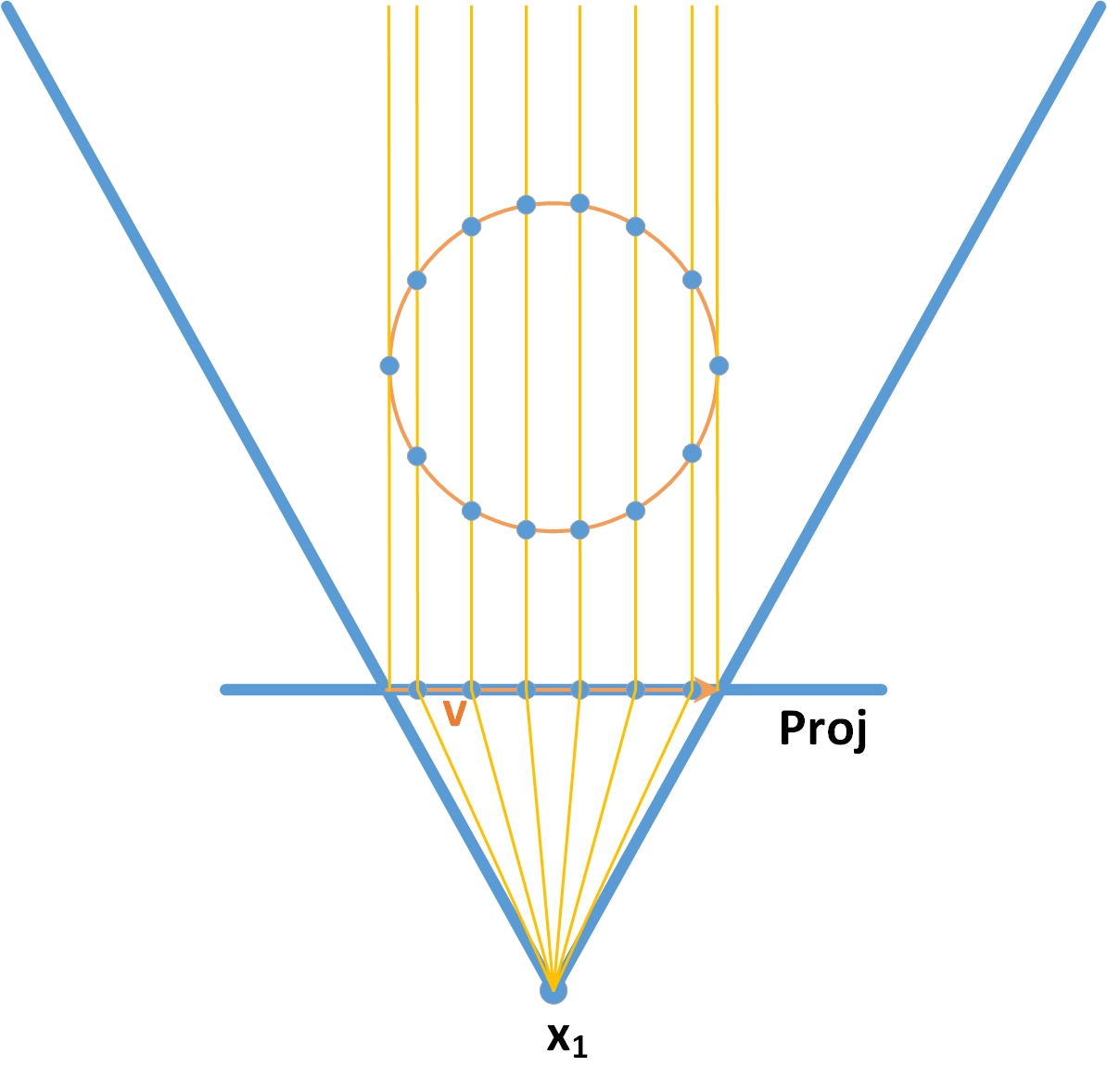
Figure 7: Direct observation (left) and parallel projection to line and observation (right).

Formally, this can be easily achieved by recalling the relation of Euclidean and polar coordinates. Then, simply extracting the $x$-part from the circular motion, we obtain trigonometric functions to describe the power series of the angle $\varphi$ correctly. Dependent on the initial point of motion/observation, we thus obtain solutions $~{}\sin\varphi$ or $~{}\cos\varphi$. However, analytically we have suppressed the fact that with respect to the right picture, the observer is no longer located in $x_{1}$, but has moved to $y=-\infty$ in order to apply the parallel projection and the related coordinate selection. So as above in the case of the parabola, the ability of the observer to distinguish linear from non-linear motion depends not only on parameters of the observed objects (e.g. in the case of a very large radius) but also on the experimental setup and the quality of the observation process.

The observation improves, and it’s much easier to identify the original process, if we move the observer from $\infty$ towards the projection line ’Proj’. Now, the lines of the ’observer pencil’ loose their parallel character more and more, the closer the observer approaches the projection line, or the center of the circle with uniform motion, respectively. So with uniform angular motion, the circular motion of the point to the one side (or direction) differs more and more from the motion to the other side/direction. Once more, the ’distortion effect’ depends on the distance of the orbit to the projection line ’Proj’.

Nevertheless, both processes should be treated consistently in terms of line pencils and their related geometry. This can be seen even better if – as above – we move the center of the ’observer line pencil’ beyond the projection line, or even into the orbit(s) of the motion, i.e. close to the center of the circular motion.

Last not least, we may mention the case of the circular motion (or the linearization as mathematical pendulum) as physical process, and a 1-dim oscillator (or the spring, respectively) on ’Proj’.

So as discussed already above, the information difference between the circular motion and the projection onto the line ’Proj’ is apparent if we consider the case of parallel projection, i.e. we position the observer $x_{1}$ at the position $y\longrightarrow\infty$ in terms of Euclidean coordinates (or at the ’absolute line’ $x_{0}=0$ of the plane in homogeneous coordinates).

The two related ’physical’ scenarios can be summarized by the circular planar motion with constant angular velocity on the one hand, and the picture of a 1-dim oscillation (or spring) on the other hand in order to describe the motion of the projected point. Formally, within this Euclidean setup, we may just neglect the $y$-coordinate of the circular motion by appropriately chosen origin in the center of the circular motion. This may be also presented in the ’linearized’ versions of the pendulum and the spring. In all cases, however, we have to re-identify and rename the constants of both pictures – the full process and the projected oscillation – with respect to their respective physical meaning.

So the parameters of the rotating point/the pendulum and the spring reflect in a mapping of length and angular velocity onto effective parameters ’mass’ and ’spring constant’ in the ’Proj’ description, and we may use the dynamical picture of the rotating point to ’enhance’ the picture of the spring. Of course, both physical processes exist, and nobody would describe springs and Hooke’s law by a formally equivalent description in terms of a 2-dim rotation without need.

References

- (1) Bjorken J D, Drell S D 1965 Relativistic Quantum Mechanics. (New York: McGraw-Hill)
- (2) Blaschke W 1928 Vorlesungen über Differentialgeometrie III. (Die Grundlehren der mathematischen Wissenschaft XXIX) (Berlin: Springer)
- (3) Wiegand R 2008 Ein streitbarer Gelehrter im 19. Jahrhundert. http://www3.uni-bonn.de/Pressemitteilungen/ein-streitbarer-gelehrter-im-19-jahrhundert (Pressemitteilungen, 21.5.2008) (University Bonn: Pressestelle)
- (4) Clebsch A 1871 Zum Gedächtniss an Julius Plücker. Abhandlungen der Königlichen Gesellschaft der Wissenschaften zu Göttingen 16
- (5) Clebsch A 1869 Ueber die Plückerschen Complexe. Math. Ann. 2 1
- (6) Dahm R 2012 On A Microscopic Representation of Space-Time. Yad. Fis. 75 1244; Phys. Atom. Nuclei 75 1173; Proceedings of SymPhys XIV, Tsaghkadzor
- (7) Dahm R 2011 On A Microscopic Representation of Space-Time II. Proceedings of ICCA 9, Weimar, 2011; to be published
- (8) Dahm R 2011 Projective Geometry, Conformal and Lie Symmetries and Their Breakdown to a su(2)u(1) Lie Algebra. QTS 7, Prague, 2011
- (9) Dahm R 2013 Some Remarks on Rank-3 Lie Algebras in Physics. GOL X, Tallinn, 2013
- (10) Dahm R 2018 On a Microscopic Representation of Space-Time VII – On Spin. J. Phys.: Conf. Ser. 965 012012
- (11) Dahm R 2018 On a Microscopic Representation of Space-Time VIII – On Relativity. Yad. Fis./Phys. Atom. Nuclei, accepted for publication
- (12) Ehlers J, Pirani F and Schild A 1972 The Geometry of Free Fall and Light Propagation. In: Studies in Relativity. ed L O’Raifeartaigh (Oxford: Clarendon Press) pp 63–84
- (13) Enriques F 1903 Vorlesungen über Projektive Geometrie. (Leipzig: B. G. Teubner)
- (14) Gilmore R 1974 Lie Groups, Lie Algebras and Some of Their Applications (New York: John Wiley & Sons)
- (15) Helgason S 1978 Differential Geometry, Lie Groups, and Symmetric Spaces (San Diego: Academic Press)
- (16) Jackson J D 1983 Klassische Elektrodynamik. 2nd edition (1975, German translation) (Berlin: de Gruyter)
- (17) Kähler E 1960 Innerer und Äusserer Differentialkalkül. Abhandlungen der Deutschen Akademie der Wissenschaften zu Berlin (Berlin: Akademie-Verlag)
- (18) Klein F 1868 Ueber die Transformation der allgemeinen Gleichung des zweiten Grades zwischen Linien-Koordinaten auf eine kanonische Form. Inauguraldissertation (Bonn: Georgi)
- (19) Klein F 1872 Ueber Liniengeometrie und metrische Geometrie. Math. Ann. 5 257
- (20) Klein F 1872 Ueber gewisse in der Liniengeometrie auftretende Differentialgleichungen. Math. Ann. 5 278
- (21) Klein F 1872 Zur Interpretation der complexen Elemente in der Geometrie. Göttinger Nachrichten 1872, p. 373
- (22) Klein F 1928 Vorlesungen über nicht-euklidische Geometrie. (Die Grundlehren der mathematischen Wissenschaft XXVI) (Berlin: Springer)
- (23) Lurié D 1968 Particles and Fields. (New York, London, Sydney: Interscience Publishers)
- (24) Percacci R 1986 Geometry of Nonlinear Field Theories. (Singapore: World Scientific)
- (25) Plücker J 1838 Discussion de la forme générale des ondes lumineuses. Journal für die reine und angewandte Mathematik 19 1; ibd. 19 91
- (26) Plücker J 1865 On a New Geometry of Space. Proc. Royal Soc. London 14 58
- (27) Plücker J 1866 Fundamental Views regarding Mechanics. Phil. Transactions Royal Soc. London 156 361
- (28) Plücker J 1868/1869 Neue Geometrie des Raumes. ed A Clebsch and F Klein (Leipzig: B. G. Teubner)
- (29) Reye Th 1866/1868 Die Geometrie der Lage. (Hannover: Rümpler)
- (30) Reye Th 1879 Synthetische Geometrie der Kugeln und linearen Kugelsysteme. (Leipzig: Teubner)
- (31) Smilga W 2011 Reverse Engineering Approach to Quantum Electrodynamics. arXiv:1004.0820 [physics.gen-ph]
- (32) Study E 1903 Geometrie der Dynamen. (Leipzig: Teubner)
- (33) von Staudt G K C 1856 Beiträge zur Geometrie der Lage. (Nürnberg: Bauer und Raspe)
- (34) H. Weyl, Raum-Zeit-Materie. (6th ed. Berlin Heidelberg New York: Springer, 1970 (1918))
- (35) Zindler K 1902/1906. Liniengeometrie mit Anwendungen. (Sammlung Schubert XXXIV/LI) (Leipzig: G. J. Göschensche Verlagshandlung)