A model-independent analysis of final-state interactions in $\bar{B}_{d/s}^{0}\to J/\psi\pi\pi$

Abstract

Exploiting $B$-meson decays for Standard Model tests and beyond requires a precise understanding of the strong final-state interactions that can be provided model-independently by means of dispersion theory. This formalism allows one to deduce the universal pion–pion final-state interactions from the accurately known $\pi\pi$ phase shifts and, in the scalar sector, a coupled-channel treatment with the kaon–antikaon system. In this work an analysis of the decays $\bar{B}_{d}^{0}\to J/\psi\pi^{+}\pi^{-}$ and $\bar{B}_{s}^{0}\to J/\psi\pi^{+}\pi^{-}$ is presented. We find very good agreement with the data up to 1.05 GeV in the $\pi\pi$ invariant mass, with a number of parameters reduced significantly compared to a phenomenological analysis. In addition, the phases of the amplitudes are correct by construction, a crucial feature for many $CP$ violation measurements in heavy-meson decays.

1 Introduction

$B$-meson decays can be exploited for Standard Model tests and beyond, in particular to determine the Cabibbo–Kobayashi–Maskawa (CKM) couplings and to study $CP$ violation. For a theoretical description of many of these decays, it is mandatory to understand the strong final-state interactions in terms of amplitude analysis techniques Battaglieri:2014gca , with tight control over the magnitudes and phase motions of the various partial waves involved. For example, the decays $B\to f_{0}(980)K_{S}$ and $B\to\phi(1020)K_{S}$ are explored for an experimental determination of the $CP$ asymmetry $\sin 2\beta$ Dalseno:2008wwa ; Aubert:2009me ; Nakahama:2010nj ; Lees:2012kxa , $\beta$ being one of the angles of the unitarity triangle, which requires precise knowledge of the strange and non-strange scalar form factors that we discuss in this article. We focus on the decays $\bar{B}_{d}^{0}\to J/\psi\pi^{+}\pi^{-}$ and $\bar{B}_{s}^{0}\to J/\psi\pi^{+}\pi^{-}$, measured by the LHCb collaboration Aaij:2014siy ; Aaij:2014emv . The tree-level process of the weak decay into $J/\psi$ and a $q\bar{q}$ pair is depicted in Fig. 1 (exemplarily for the $\bar{B}_{s}^{0}$ decay).

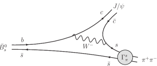
Figure 1: The $\bar{B}_{s}^{0}\to J/\psi\pi^{+}\pi^{-}$ diagram to leading order via $W^{-}$ exchange. The hadronization into pions ($S$-wave dominated) proceeds through the pion strange scalar form factor $\Gamma^{s}_{\pi}(s)$. In the case of the $\bar{B}_{d}^{0}\to J/\psi\pi^{+}\pi^{-}$ decay, with $s\leftrightarrow d$, the pions are generated out of a non-strange scalar source, i.e. $\Gamma^{s}_{\pi}(s)$ is replaced by the pion non-strange scalar form factor $\Gamma^{n}_{\pi}(s)$ for $S$-wave and by the vector form factor for $P$-wave pions.

These analyses complement former related studies of $\bar{B}_{d}^{0}$ and $\bar{B}_{s}^{0}$ decays by the BaBar Aubert:2002vb , Belle Li:2011pg , CDF Aaltonen:2011nk , and D0 Abazov:2011hv Collaborations as well as older LHCb results Aaij:2013zpt ; LHCb:2012ae . Universality of final-state interactions dictates that the hadronization into pions and the rescattering effects in the $\pi^{+}\pi^{-}$ system for $S$- and $P$-waves are closely related to the scalar and vector pion form factors, respectively. We describe these form factors using dispersion theory, using Omnès (or Muskhelishvili–Omnès) representations. In doing so we exploit the fact that LHCb found no obvious structures in the $J/\psi\pi^{+}$ invariant mass distribution, suggesting that left-hand-cut contributions in the $\pi^{+}\pi^{-}$ system due to the crossed-channel $J/\psi\pi^{+}$ interaction are small and can be neglected.

The advantage of the dispersive framework is that all constraints imposed by analyticity (i.e., causality) and unitarity (probability conservation) are fulfilled by construction. Further, it is a model-independent approach, so we do not have to specify any contributing resonances or conceivable non-resonant backgrounds. For the vector form factor a single-channel (elastic) treatment works very well below 1 . In the scalar sector the strong coupling of two $S$-wave pions to $K\bar{K}$ near 1  due to the $f_{0}(980)$ resonance, causing a sharp onset of the $K\bar{K}$ inelasticity, necessitates a coupled-channel treatment. Therefore a two-channel Muskhelishvili–Omnès problem is solved. This two-channel approach breaks down at energies where inelasticities caused by $4\pi$ states become important, we are thus not able to cover the complete phase space, but restrict ourselves to the low-energy range $\sqrt{s}\leq 1.05~{}$.

In Ref. Aaij:2014siy the $\bar{B}_{d}^{0}$ decay is described by six resonances in the $\pi^{+}\pi^{-}$ channel, $f_{0}(500)$, $\rho(770)$, $\omega(782)$, $\rho(1450)$, $\rho(1700)$, and $f_{2}(1270)$, which are modeled by Breit–Wigner functions. This parametrization of especially the $f_{0}(500)$ meson is somewhat precarious, as the broad bump structure of this scalar resonance is not well described by a Breit–Wigner shape. As demonstrated for the first time in the context of $B$ decays in Ref. Gardner:2001gc , it should be replaced by the corresponding scalar form factor. In the present work this idea is extended and rigorously applied using form factors derived from dispersion theory. In particular, there is no need to parametrize any resonance, since the input required to describe the final-state interactions is taken from known phase shifts, and therefore the $f_{0}(500)$ appears naturally in the non-strange scalar form factor. The $\bar{B}_{s}^{0}$ decay, described in the experimental analysis by five resonances, $f_{0}(980)$, $f_{0}(1500)$, $f_{0}(1790)$, $f_{2}(1270)$, and $f_{2}^{\prime}(1525)$ (Solution I) or with an additional non-resonant contribution (Solution II), dominantly occurs in an $S$-wave state Aaij:2014emv , while the $P$-wave is shown to be negligible. Given the almost pure $\bar{s}s$ source the pions are generated from, this decay shows great promise to provide insight into the strange scalar form factor.

The idea of such a “scalar-source model”, where an $S$-wave pion pair is generated out of a quark–antiquark pair and the final-state interactions are described by the scalar form factor, is also used in Ref. Liang:2014tia for the description of the $\bar{B}_{s}^{0}$ and $\bar{B}_{d}^{0}$ decays into the scalar resonances $f_{0}(980)$ and $f_{0}(500)$, respectively. It was employed earlier e.g. in analyses of the decay of the $J/\psi$ into a vector meson ($\omega$ or $\phi$) and a pair of pseudoscalars ($\pi\pi$ or $K\bar{K}$) Meissner:2000bc ; Lahde:2006wr . In these references the strong-interaction part is described by a chiral unitary theory including coupled channels, which yields a dynamical generation of the scalar mesons. In contrast to the present study, the very precise information available on pion–pion Ananthanarayan:2000ht ; GarciaMartin:2011cn ; CCL2012 ; CCLprep and pion–kaon BDM04 phase shifts is not strictly implemented there. Related studies using the chiral unitary approach are performed in Ref. Bayar:2014qha , where the $J/\psi$–vector-meson final state is analyzed, and in Ref. Xie:2014gla , which includes resonances beyond 1 . In contrast to models of dynamical resonance generation, the scalar resonances are considered as $q\bar{q}$ or tetraquark states in Ref. Stone:2013eaa . Other theoretical approaches employ light-cone QCD sum rules to describe the form factors Colangelo:2010bg . Progress on the short-distance level is made in Ref. Wang:2015uea , where the factorization formulae (which we treat in a naive way) are improved in a perturbative QCD framework.

This manuscript is organized as follows. In Sec. 2, we review the construction of the transversity amplitudes and partial waves, after sketching the kinematics. We provide explicit expressions that relate the theoretical quantities to the angular moments determined in experiment. Section 3 is focused on the Omnès formalism. The fits to the LHCb data, using the $\bar{B}_{d/s}^{0}\to J/\psi\pi^{+}\pi^{-}$ angular moment distributions, are discussed in Sec. 4, where we use several configurations with and without $D$-wave corrections to study the impact of certain corrections to our fits. We also predict the $S$-wave amplitude for the related $\bar{B}_{s}^{0}\to J/\psi K^{+}K^{-}$ decay. The paper ends with a summary and an outlook in Sec. 5. Some technical details are relegated to the appendices.

2 Kinematics, decay rate, and angular moments

In this section we derive the decay rate and angular moments for the $\bar{B}_{d}^{0}\to J/\psi\pi^{+}\pi^{-}$ decay mode in terms of partial-wave amplitudes up to $D$-waves, employing the transversity formalism of Ref. Faller:2013dwa . The formalism works analogously for the $\bar{B}_{s}^{0}$ decay.

2.1 Kinematics

The kinematics of the decay $\bar{B}_{d/s}^{0}(p_{B})\to J/\psi(p_{\psi})\pi^{+}(p_{1})\pi^{-}(p_{2})$ ($J/\psi\to\mu^{+}\mu^{-}$) can be described by four variables:

• the invariant dimeson mass squared, $s=(p_{1}+p_{2})^{2}$,

and three helicity angles, see Fig. 2,

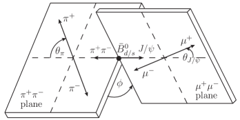
Figure 2: Definition of the kinematical variables for $\bar{B}_{d/s}^{0}\to J/\psi\pi^{+}\pi^{-}$.

• $\theta_{J/\psi}$, the angle between the $\mu^{+}$ in the $J/\psi$ rest frame ($\Sigma_{J/\psi}$) and the $J/\psi$ in the $\bar{B}_{d/s}^{0}$ rest frame ($\Sigma_{B}$);

• $\theta_{\pi}$, the angle between the $\pi^{+}$ in the $\pi^{+}\pi^{-}$ center-of-mass frame $\Sigma_{\pi\pi}$ and the dipion line-of-flight in $\Sigma_{B}$;

• $\phi$, the angle between the dipion and the dimuon planes, where the latter originate from the decay of the $J/\psi$.

The three-momenta of either of the two pions in the dipion center-of-mass system ($\mathbf{p}_{\pi}$) and of the $J/\psi$ in the $\bar{B}_{d/s}^{0}$ rest frame ($\mathbf{p}_{\psi}$) are given by

$$|\mathbf{p}_{\pi}|=\frac{\lambda^{1/2}(s,M_{\pi}^{2},M_{\pi}^{2})}{2\sqrt{s}}\equiv\frac{\sigma_{\pi}\sqrt{s}}{2},\quad|\mathbf{p}_{\psi}|=\frac{\lambda^{1/2}(s,m_{\psi}^{2},m_{B}^{2})}{2m_{B}}\equiv\frac{X}{m_{B}},$$ (2.1)

with the Källén function $\lambda(a,b,c)=a^{2}+b^{2}+c^{2}-2ab-2ac-2bc$.

We define the two remaining Mandelstam variables as

$$t=(p_{B}-p_{1})^{2}\quad{\rm and}\quad u=(p_{B}-p_{2})^{2},$$ (2.2)

where the difference of these two determines the scattering angle $\theta_{\pi}$,

$$t-u=-2p_{\psi}(p_{1}-p_{2})=-2\sigma_{\pi}X\cos\theta_{\pi}.$$ (2.3)

Further, we introduce two additional vectors as combinations of the above four-momenta,

$$P^{\mu}=p_{1}^{\mu}+p_{2}^{\mu},\quad Q^{\mu}=p_{1}^{\mu}-p_{2}^{\mu}.$$ (2.4)

2.2 Matrix element

To calculate the matrix element we make use of the effective Hamiltonian that governs the $b\to c\bar{c}d$ transition Buchalla:1995vs ,

$$\mathcal{H}_{\rm eff}=\frac{G_{F}}{\sqrt{2}}\big{\{}V_{cb}V^{*}_{cd}\left[C_{1}(\mu)O_{1}(\mu)+C_{2}(\mu)O_{2}(\mu)\right]+\dots\big{\}},$$ (2.5)

where the $C_{i}$ are Wilson coefficients and the $O_{i}$ local current–current operators

$$O_{1} = \bar{c}_{k}\gamma_{\mu}(1-\gamma_{5})b_{l}\,\,\bar{d}_{l}\gamma^{\mu}(1-\gamma_{5})c_{k}=\bar{c}_{k}\gamma_{\mu}(1-\gamma_{5})c_{k}\,\,\bar{d}_{l}\gamma^{\mu}(1-\gamma_{5})b_{l},$$

$$O_{2} = \bar{c}_{k}\gamma_{\mu}(1-\gamma_{5})b_{k}\,\,\bar{d}_{l}\gamma^{\mu}(1-\gamma_{5})c_{l}=\bar{c}_{k}\gamma_{\mu}(1-\gamma_{5})c_{l}\,\,\bar{d}_{l}\gamma^{\mu}(1-\gamma_{5})b_{k},$$ (2.6)

with $k,l$ being color indices. In the second step the quark operators are regrouped by means of a Fierz rearrangement. The ellipses in $\mathcal{H}_{\rm eff}$ denote operators beyond tree-level, including penguin topologies. $V_{cb}$ and $V_{cd}$ are the CKM matrix elements for $c\to b$ and $c\to d$ (where $V_{cd}$ is to be replaced by $V_{cs}$ for the $\bar{B}_{s}^{0}$ decay), and $G_{F}=1.166365\times 10^{-5}~{}^{-2}$ is the Fermi constant.

Under the assumption that the final-state interaction between the $J/\psi$ and the pions is negligible (no obvious structures are found in the $J/\psi\pi$ channel experimentally Aaij:2014siy ; Aaij:2014emv , and a close-to-zero $J/\psi\pi$ scattering length $a_{J/\psi\pi}=-0.01(1)$ fm results from lattice calculations Liu:2008rza ) a factorization approach appears to be justified. Note that on the quark level this naive factorization ansatz may be spoiled Beneke:2000ry ; Diehl:2001xe , for instance due to (large) penguin contributions that we have neglected in Eq. (2.5) Aaij:2014vda ; Frings:2015eva . However, a more complicated structure of the source term does not conflict with our approach: any factorization limitations due to color structures do not concern the hadronic final-state interaction, for which the short-distance factorizations are sufficient but not mandatory. All we use is the fact that the $B$ decays provide clean $\bar{q}q$ sources of much shorter range than that of the final-state interaction. In our approach, any deviations from clean point sources would be parametrized by derivatives of the source term. An excellent fit to the data even without those correction terms is a proof that with respect to the final-state interactions the sources can be regarded as point-like.

We express the matrix elements of the four-quark operators by two independent hadronic currents, valid if the $c\bar{c}$ system produced by the hadronization of the virtual $W^{-}$ is well separated from the spectator quark system. For the decay of the $\bar{B}_{d}^{0}$ meson considered here the matrix element is, in analogy to the $\bar{B}_{s}^{0}$ expression given in Ref. Colangelo:2010wg , written as

$$\mathcal{M}_{fi} = \frac{G_{F}}{\sqrt{2}}V_{cb}V_{cd}^{*}\,a^{\rm eff}(\mu)\underbrace{\langle\pi^{+}(p_{1})\pi^{-}(p_{2})|\bar{d}\gamma_{\mu}(1-\gamma_{5})b|\bar{B}_{d/s}^{0}(p_{B})\rangle}_{\mathcal{M}^{\pi\pi}_{\mu}}\times\underbrace{\langle J/\psi(p_{\psi},\epsilon)|\bar{c}\gamma^{\mu}c|0\rangle}_{\mathcal{M}^{c\bar{c}\,\mu}},$$

$$\mathcal{M}^{\pi\pi}_{\mu} = \frac{M_{\psi}P_{(0)}^{\mu}}{X}\mathcal{F}_{0}+\frac{Q_{(\parallel)}^{\mu}}{\sqrt{s}}\mathcal{F}_{\parallel}-\frac{i\bar{p}_{\perp}^{\mu}}{\sqrt{s}}\mathcal{F}_{\perp},\qquad\mathcal{M}^{c\bar{c}}_{\mu}=f_{\psi}M_{\psi}\epsilon_{\mu}^{*}(p_{\psi},\lambda),$$ (2.7)

with $a^{\rm eff}=C_{1}(\mu)+C_{2}(\mu)/N_{c}+\dots$, the ellipses denoting combinations of Wilson coefficients due to penguin diagrams, we have not taken into account explicitly.

The scale ($\mu$) dependence of the Wilson coefficients is cancelled by the scale dependence of the hadronic matrix elements, cf. Sec. 3; $\mu$ is chosen to be of order $\mathcal{O}(m_{B})$, such that heavier particles, in particular the $W$, are integrated out.

The current that creates the $J/\psi$ from the vacuum is related to the decay constant $f_{\psi}$. The matrix element containing the pions is given by the three transversity form factors $\mathcal{F}_{0}$, $\mathcal{F}_{\parallel}$, and $\mathcal{F}_{\perp}$, corresponding to the orthogonal basis of momentum vectors Faller:2013dwa

$$p_{\psi}^{\mu},\quad\bar{p}_{(\perp)}^{\mu}=\frac{\epsilon^{\mu\alpha\beta\gamma}}{X}(p_{\psi})_{\alpha}P_{\beta}Q_{\gamma},\quad Q_{(\parallel)}^{\mu}=Q^{\mu}-\frac{(P\cdot p_{\psi})(Q\cdot p_{\psi})}{X^{2}}P^{\mu}+\frac{s(Q\cdot p_{\psi})}{X^{2}}p_{\psi}^{\mu}.$$ (2.8)

We define $\epsilon_{\mu\nu\rho\sigma}$ such that $\epsilon_{0123}=-\epsilon^{0123}=+1$.

The partial-wave expansions of the transversity form factors read

$$\mathcal{F}_{0}(s,\theta_{\pi}) =\sum_{\ell}\sqrt{2\ell+1}\,\mathcal{F}_{0}^{(\ell)}(s)P_{\ell}(\cos\theta_{\pi})$$

$$=\mathcal{F}_{0}^{(S)}(s)+\sqrt{3}\cos\theta_{\pi}\mathcal{F}_{0}^{(P)}(s)+\frac{\sqrt{5}}{2}\left(3\cos^{2}\theta_{\pi}-1\right)\mathcal{F}_{0}^{(D)}(s)+\dots\,,$$

$$\mathcal{F}_{\parallel,\perp}(s,\theta_{\pi}) =\sum_{\ell}\frac{\sqrt{2\ell+1}}{\sqrt{\ell(\ell+1)}}\mathcal{F}_{\parallel,\perp}^{(\ell)}(s)P_{\ell}^{\prime}(\cos\theta_{\pi})=\sqrt{\frac{3}{2}}\left(\mathcal{F}_{\parallel,\perp}^{(P)}(s)+\sqrt{5}\cos\theta_{\pi}\mathcal{F}_{\parallel,\perp}^{(D)}(s)\right)+\dots,$$ (2.9)

where the ellipses denote waves larger than $D$-waves. In Appendix A the relation to the helicity form factors is briefly sketched, which have a well-known partial-wave expansion.

2.3 Decay rate and angular moments

When comparing the angular moments to the experimental data we have to deal with flavor-averaged expressions due to the $B^{0}$–$\bar{B}^{0}$ mixing and take into account the $CP$-conjugated amplitudes (the $B_{d}^{0}$ decay mode) as well. Since the interfering term between the amplitudes is negligibly small Aaij:2014siy , the decay rate can be written as the sum of the decay rates for the direct $\bar{B}_{d}^{0}$ and the mixed $CP$-conjugated $B_{d}^{0}$ mode,

$$\frac{{\text{d}}^{2}\Gamma\left(\bar{B}_{d}^{0}\to J/\psi\pi^{+}\pi^{-}\right)}{{\text{d}}\sqrt{s}\,{\text{d}}\cos\theta_{\pi}}\approx\frac{{\text{d}}^{2}\Gamma\left({\rm direct}\right)}{{\text{d}}\sqrt{s}\,{\text{d}}\cos\theta_{\pi}}+\frac{{\text{d}}^{2}\Gamma\left(B_{d}^{0}\to J/\psi\pi^{+}\pi^{-}\right)}{{\text{d}}\sqrt{s}\,{\text{d}}\cos\theta_{\pi}}.$$ (2.10)

Note that this neglect is less justified when applying the formulae to the $\bar{B}_{s}^{0}$ decay rate. In the analysis of Ref. Aaij:2014emv an interference term is added to Eq. (2.10). However, in Sec. 4.2 we find that it is sufficient to take into account $S$-waves. In that case the interference term does not affect the fit procedure and merely generates a tiny shift of the resulting fit parameter (the normalization $c_{0}^{s}$).

In this section we provide expressions for one particular mode. The $CP$-related amplitude can be deduced straightforwardly by multiplying the transversity partial-wave amplitudes with $CP$ eigenvalues as outlined in detail below (cf. the discussion around Eq. (2.15)).

The differential decay rate is given by

$$\frac{{\text{d}}^{2}\Gamma}{{\text{d}}\sqrt{s}\,{\text{d}}\cos\theta_{\pi}} =\frac{G_{F}^{2}|V_{cb}|^{2}|V_{cd}|^{2}f_{\psi}^{2}M_{\psi}^{2}X\sigma_{\pi}\sqrt{s}}{4(4\pi)^{3}m_{B}^{3}}$$

$$\times\bigg{\{}\Big{|}\mathcal{F}_{0}^{(S)}(s)+\sqrt{3}\cos\theta_{\pi}\mathcal{F}_{0}^{(P)}(s)+\frac{\sqrt{5}}{2}\left(3\cos^{2}\theta_{\pi}-1\right)\mathcal{F}_{0}^{(D)}(s)\Big{|}^{2}$$

$$+\frac{3}{2}\sigma_{\pi}^{2}\sin^{2}\theta_{\pi}\bigg{(}\Big{|}\mathcal{F}_{\parallel}^{(P)}+\sqrt{5}\cos\theta_{\pi}\mathcal{F}_{\parallel}^{(D)}(s)\Big{|}^{2}+\Big{|}\mathcal{F}_{\perp}^{(P)}+\sqrt{5}\cos\theta_{\pi}\mathcal{F}_{\perp}^{(D)}(s)\Big{|}^{2}\bigg{)}\bigg{\}},$$ (2.11)

see Appendix A for details. By weighting this decay rate by spherical harmonic functions $Y_{l}^{0}(\cos\theta_{\pi})$, we define the angular moments

$$\langle Y_{l}^{0}\rangle(s)=\int_{-1}^{1}\frac{{\text{d}}^{2}\Gamma}{{\text{d}}\sqrt{s}\,{\text{d}}\cos\theta_{\pi}}Y_{l}^{0}(\cos\theta_{\pi}){\text{d}}\cos\theta_{\pi}.$$ (2.12)

With the orthogonality property

$$\int_{-1}^{1}Y_{i}^{0}(\cos\theta_{\pi})Y_{j}^{0}(\cos\theta_{\pi}){\text{d}}\cos\theta_{\pi}=\frac{\delta_{ij}}{2\pi},$$ (2.13)

we obtain

$$\sqrt{4\pi}\langle Y_{0}^{0}\rangle =\frac{G_{F}^{2}|V_{cb}|^{2}|V_{cd}|^{2}f_{\psi}^{2}M_{\psi}^{2}X\sigma_{\pi}\sqrt{s}}{2(4\pi)^{3}m_{B}^{3}}\bigg{\{}\Big{|}\mathcal{F}_{0}^{(S)}\Big{|}^{2}+\Big{|}\mathcal{F}_{0}^{(P)}\Big{|}^{2}+\Big{|}\mathcal{F}_{0}^{(D)}\Big{|}^{2}$$

$$\quad+\sigma_{\pi}^{2}\bigg{(}\Big{|}\mathcal{F}_{\parallel}^{(P)}\Big{|}^{2}+\Big{|}\mathcal{F}_{\perp}^{(P)}\Big{|}^{2}+\Big{|}\mathcal{F}_{\parallel}^{(D)}\Big{|}^{2}+\Big{|}\mathcal{F}_{\perp}^{(D)}\Big{|}^{2}\bigg{)}\bigg{\}},$$

$$\sqrt{4\pi}\langle Y_{1}^{0}\rangle =\frac{G_{F}^{2}|V_{cb}|^{2}|V_{cd}|^{2}f_{\psi}^{2}M_{\psi}^{2}X\sigma_{\pi}\sqrt{s}}{(4\pi)^{3}m_{B}^{3}}\bigg{\{}\text{Re}\,\Big{(}\mathcal{F}_{0}^{(S)}\mathcal{F}_{0}^{(P)^{*}}\Big{)}+\frac{2}{\sqrt{5}}\text{Re}\,\Big{(}\mathcal{F}_{0}^{(P)}\mathcal{F}_{0}^{(D)^{*}}\Big{)}$$

$$\quad+\sqrt{\frac{3}{5}}\sigma_{\pi}^{2}\bigg{[}\text{Re}\,\Big{(}\mathcal{F}_{\perp}^{(P)}\mathcal{F}_{\perp}^{(D)^{*}}\Big{)}+\text{Re}\,\Big{(}\mathcal{F}_{\parallel}^{(P)}\mathcal{F}_{\parallel}^{(D)^{*}}\Big{)}\bigg{]}\bigg{\}},$$

$$\sqrt{4\pi}\langle Y_{2}^{0}\rangle =\frac{G_{F}^{2}|V_{cb}|^{2}|V_{cd}|^{2}f_{\psi}^{2}M_{\psi}^{2}X\sigma_{\pi}\sqrt{s}}{(4\pi)^{3}m_{B}^{3}}\bigg{\{}\text{Re}\,\Big{(}\mathcal{F}_{0}^{(S)}\mathcal{F}_{0}^{(D)^{*}}\Big{)}+\frac{1}{\sqrt{5}}\Big{|}\mathcal{F}_{0}^{(P)}\Big{|}^{2}+\frac{\sqrt{5}}{7}\Big{|}\mathcal{F}_{0}^{(D)}\Big{|}^{2}$$

$$\quad-\frac{\sigma_{\pi}^{2}}{2\sqrt{5}}\bigg{(}\Big{|}\mathcal{F}_{\parallel}^{(P)}\Big{|}^{2}+\Big{|}\mathcal{F}_{\perp}^{(P)}\Big{|}^{2}\bigg{)}+\frac{\sigma_{\pi}^{2}\sqrt{5}}{14}\bigg{(}\Big{|}\mathcal{F}_{\parallel}^{(D)}\Big{|}^{2}+\Big{|}\mathcal{F}_{\perp}^{(D)}\Big{|}^{2}\bigg{)}\bigg{\}},$$ (2.14)

where $\langle Y_{0}^{0}\rangle$ corresponds to the event distribution, $\langle Y_{1}^{0}\rangle$ describes the interference between $S$- and $P$-wave as well as $P$- and $D$-wave amplitudes, and $\langle Y_{2}^{0}\rangle$ contains $P$-wave, $D$-wave, and $S$–$D$-wave interference contributions.

The corresponding expressions for the $CP$-conjugated modes are related to the above equations by certain sign changes due to the $CP$ eigenvalues $\eta_{CP}=\pm 1$ in the definitions of the transversity partial-wave amplitudes, as already mentioned in the beginning of this section. We declare the amplitudes $\mathcal{F}_{\tau}^{(\ell)}$ to describe the $B_{d}^{0}$ decay, then the corresponding $\bar{B}_{d}^{0}$ decay amplitudes are given by

$$\bar{\mathcal{F}}_{\tau}^{(\ell)}=\eta_{CP}\mathcal{F}_{\tau}^{(\ell)},$$ (2.15)

with $\eta_{CP}=+1$ for the $\tau=0,\parallel$ $P$-waves and the $\tau=\perp$ $D$-wave, and $\eta_{CP}=-1$ otherwise. Consequently the angular moments $\langle Y_{0}^{0}\rangle$ and $\langle Y_{2}^{0}\rangle$ are unchanged under $CP$ conjugation, while the conjugated moment $\langle Y_{1}^{0}\rangle$ has opposite sign, such that when considering flavor-averaged quantities and summing over the $B_{d}^{0}$ and $\bar{B}_{d}^{0}$ contributions, $\langle Y_{1}^{0}\rangle$ vanishes. In the following we thus consider $\langle Y_{0}^{0}\rangle$ and $\langle Y_{2}^{0}\rangle$ only.

3 Omnès formalism

We describe the $S$- and $P$-wave amplitudes using dispersion theory. This approach allows us to treat the pion–pion rescattering effects in a model-independent way, based on the fundamental principles of unitarity and analyticity: the partial waves are analytic functions in the whole $s$-plane except for a branch-cut structure dictated by unitarity. In the following we deal with the functions $f_{\ell}^{I}(s)$ (referring to isospin $I$ and angular momentum $\ell$) that possess a right-hand cut starting at the pion–pion threshold $s_{\rm thr}=4M_{\pi}^{2}$ and are analytic elsewhere, i.e. we do not consider any left-hand-cut or pole structure related to crossing symmetry. This is justified from the observation that there are practically no structures observed for the crossed $J/\psi\pi^{+}$ channel in the region of interest Aaij:2014siy .

Considering two-pion intermediate states only, Watson’s theorem holds, i.e. the phase of the partial wave is given by the elastic pion–pion phase shift Watson:1954uc , and the discontinuity across the cut can be written as

$${\rm disc}f_{\ell}^{I}(s)=f_{\ell}^{I}(s+i\epsilon)-f_{\ell}^{I}(s-i\epsilon)=2i\sigma_{\pi}f_{\ell}^{I}(s)\left[t_{\ell}^{I}(s)\right]^{*}=f_{\ell}^{I}(s)e^{-i\delta_{\ell}^{I}}\sin\delta_{\ell}^{I}.$$ (3.1)

A solution of this unitarity relation can be constructed analytically, setting (compare Ref. Heyn:1980bh )

$$f_{\ell}^{I}(s)=P(s)\Omega_{\ell}^{I}(s),$$ (3.2)

where $P(s)$ is a polynomial not fixed by unitarity, and the Omnès function $\Omega_{\ell}^{I}(s)$ is entirely determined by the phase shift $\delta_{\ell}^{I}(s)$ Omnes:1958hv ,

$$\Omega_{\ell}^{I}(s)={\rm exp}\left\{\frac{s}{\pi}\int_{s_{\rm thr}}^{\infty}\frac{\delta_{\ell}^{I}(s^{\prime})}{s^{\prime}(s^{\prime}-s-i\epsilon)}{\text{d}}s^{\prime}\right\},$$ (3.3)

with

$$\Omega_{\ell}^{I}(0)=1\quad{\rm and}\quad\Omega_{\ell}^{I}(s)\neq 0\quad\forall\;s.$$ (3.4)

The $P$-wave amplitudes can be well described in the elastic approximation up to energies of roughly 1 . The simplest possible application is the pion vector form factor $F_{\pi}^{V}(s)$,

$$\langle 0|j_{\rm em}^{\mu}(0)|\pi^{+}(p_{1})\pi^{-}(p_{2})\rangle=(p_{2}-p_{1})^{\mu}F_{\pi}^{V}(s),\quad j_{\rm em}^{\mu}=\frac{2}{3}\bar{u}\gamma^{\mu}u-\frac{1}{3}\bar{d}\gamma^{\mu}d,$$ (3.5)

which obeys a representation like (3.2) with a linear polynomial $P_{F_{\pi}^{V}}(s)=1+\alpha s$, $\alpha\approx 0.1~{}^{-2}$ Hanhart:2013vba up to $\sqrt{s}\approx 1~{}$, with the exception of a small energy region around the $\omega$ resonance that couples to the two-pion channel via isospin-violating interactions. In this context it is important to note that the electromagnetic current $j_{\rm em}^{\mu}$, introduced in Eq. (3.5), can be decomposed as

$$j_{\rm em}^{\mu}=\frac{1}{2}\big{(}\bar{u}\gamma^{\mu}u-\bar{d}\gamma^{\mu}d\big{)}+\frac{1}{6}\big{(}\bar{u}\gamma^{\mu}u+\bar{d}\gamma^{\mu}d\big{)}.$$ (3.6)

Thus it contains with the first term an isovector and with the second term an isoscalar component. The latter couples directly to the $\omega$, whose decay into $\pi^{+}\pi^{-}$ is suppressed by isospin, but enhanced by a small energy denominator (i.e., the small width of the $\omega$), hence leading to a clearly observable effect in the pion form factor Aubert:2009ad ; Ambrosino:2010bv ; Ablikim:2015lsa . Theoretically, this effect is correctly taken into account by the replacement Gardner:1997ie ; Leutwyler:2002hm ; Hanhart:2012wi

$$P_{F_{\pi}^{V}}(s)\Omega_{1}^{1}(s)\longrightarrow P_{F_{\pi}^{V}}(s)\Omega_{1}^{1}(s)\bigg{(}1+\frac{\kappa_{\rm em}\,s}{M_{\omega}^{2}-iM_{\omega}\Gamma_{\omega}-s}\bigg{)}.$$ (3.7)

Note that in case of the $\omega$ the use of a Breit–Wigner parametrization is appropriate since the $\omega$ pole is located far above the relevant decay thresholds and since $\Gamma_{\omega}=8.5$  is very small. A fit of the form factor parametrization introduced in Eq. (3.7) to the KLOE data Ambrosino:2010bv yields $\kappa_{\rm em}\approx 1.8\times 10^{-3}$. This fixes the strength of the so-called $\rho$–$\omega$ mixing amplitude phenomenologically. The isospin-violating coupling $\kappa_{\rm em}$ is of the usual size, however, near the $\omega$ peak its smallness is balanced by the factor $M_{\omega}/\Gamma_{\omega}\approx 90$ from the $\omega$ propagator, giving rise to an isospin-violating correction as large as 15% on the amplitude level, corresponding to 30% in observables due to interference with the leading term. Note also that the $\rho$–$\omega$ mixing amplitude has been pointed out to significantly enhance certain $CP$-violating asymmetries in hadronic $B$-meson decays Gardner:1997yx .

The effect of the $\omega$ on the $\bar{B}_{d}^{0}\to J/\psi\pi^{+}\pi^{-}$ decay can be related straightforwardly to that on the pion vector form factor. To see this observe that the source term for the $\pi\pi$ system is $\bar{d}d$ at tree level, see Fig. 1, such that the isospin decomposition of the corresponding vector current reads

$$\bar{d}\gamma^{\mu}d=-\frac{1}{2}\big{(}\bar{u}\gamma^{\mu}u-\bar{d}\gamma^{\mu}d\big{)}+\frac{1}{2}\big{(}\bar{u}\gamma^{\mu}u+\bar{d}\gamma^{\mu}d\big{)}.$$ (3.8)

Comparison to Eq. (3.6) shows that the relative strength of the isoscalar component differs from the electromagnetic current by a factor of $-3$, such that we will fix the $\rho$–$\omega$ mixing contribution in analogy to Eq. (3.7), but with the replacement $\kappa_{\rm em}\to\kappa=-3\kappa_{\rm em}\approx-5.4\times 10^{-3}$. Notice that this is in contrast with the experimental analysis Aaij:2014siy , where the $\omega$ contribution is fitted with free coupling constants.

The (elastic) single-channel treatment, introduced in the beginning of this section, cannot be used in the $S$-wave case: there are strong inelastic effects in the region around 1  due to the opening of the $K\bar{K}$ channel, coinciding with the $f_{0}(980)$ resonance, which affects the phase of the scalar pion form factors (see e.g. the discussion in Ref. Ananthanarayan:2004xy ). Thus the Omnès problem has to be generalized, with the Watson theorem fulfilled in the elastic region and inelastic effects included above the $K\bar{K}$ threshold. This leads to the two-channel Muskhelishvili–Omnès equations that intertwine the pion and kaon form factors, defined as

$$\left\langle\pi^{+}(p_{1})\pi^{-}(p_{2})\left|\bar{q}q\right|0\right\rangle =\mathcal{B}^{q}\Gamma_{\pi}^{q}(s),$$

$$\left\langle K^{+}(p_{1})K^{-}(p_{2})\left|\bar{q}q\right|0\right\rangle =\mathcal{B}^{q}\Gamma_{K}^{q}(s),$$ (3.9)

where the quark flavors may be either $\bar{q}q=(\bar{u}u+\bar{d}d)/2$ for the light quarks, with the superscript $q=n$ denoting the corresponding scalar form factor, or $\bar{q}q=\bar{s}s$ for strange quarks (with superscript $q=s$). Furthermore, $\mathcal{B}^{n}=M_{\pi}^{2}/(m_{u}+m_{d})$, $\mathcal{B}^{s}=(2M_{K}^{2}-M_{\pi}^{2})/(2m_{s})$. Note that the form factors $\Gamma_{\pi,K}^{q}(s)$ are invariant under the QCD renormalization group, while the hadronic matrix elements are not due to the scale dependence inherent in the factors $\mathcal{B}^{q}$. This in turn allows for the cancellation of the scale dependence in the Wilson coefficients introduced in the effective Hamiltonian of Sec. 2.

Appealing to the tree-level diagram of Fig. 1, we expect the non-strange scalar form factors to contribute dominantly in the $\bar{B}_{d}^{0}$ decay, while the strange ones should feature mainly in the corresponding decay of the $\bar{B}_{s}^{0}$. As discussed in detail below, these expectations are confirmed by the data analysis.

The Muskhelishvili–Omnès formalism is briefly reviewed in Appendix B. It requires three input functions: in addition to the $\pi\pi$ phase shift already necessary in the elastic case, modulus and phase of the $\pi\pi\to K\bar{K}$ $S$-wave amplitude also need to be known. Our main solution is based on the Roy equation analysis by the Bern group CCL2012 ; CCLprep for the $\pi\pi$ phase shift, the modulus of the $\pi\pi\to K\bar{K}$ $S$-wave as obtained from the solution of Roy–Steiner equations for $\pi K$ scattering performed in Orsay BDM04 , and its phase from partial-wave analyses Cohen ; Etkin . Alternatively, we employ the $T$-matrix constructed by Dai and Pennington (DP) in Ref. Dai:2014zta : here, a coupled-channel $K$-matrix parametrization is fitted to $\pi\pi$ data pipidata1 ; pipidata2 ; pipidata3 ; pipidata4 ; pipidata5 , and the Madrid–Kraków Roy-equation analysis GarciaMartin:2011cn is used as input; furthermore, the $K\bar{K}$ threshold region is improved by fitting also to Dalitz plot analyses of $D_{s}^{+}\to\pi^{+}\pi^{-}\pi^{+}$ Aubert:2008ao and $D_{s}^{+}\to K^{+}K^{-}\pi^{+}$ delAmoSanchez:2010yp by the BaBar Collaboration.

In addition, the channel coupling manifests itself through the fact that even in the simplest case, corresponding to the polynomial of Eq. (3.2) reducing to a constant, the scalar form factors depend on two such constants, corresponding to the form factor normalizations for both pion and kaon. In contrast to the single-channel case, here the shape of the resulting form factors depends on the relative size of these two normalization constants; on the other hand, once this relative strength is fixed, it relates the final states $\pi\pi$ and $K\bar{K}$ to each other unambiguously. We will make use of this additional predictiveness in Sec. 4.3.

In order to apply this formalism to the transversity partial waves we have to construct partial waves $f_{\tau}^{(\ell)}(s)$ that are free of kinematical singularities, i.e. represented by functions whose only non-analytic behavior is related to unitarity. In Appendix A the hadronic matrix element is introduced (using the basis of the momenta $p_{\psi}^{\mu}$, $P^{\mu}$, and $Q^{\mu}$, Eq. (2.4)) in terms of the form factors $\mathcal{A}_{i}$ and $\mathcal{V}$, Eq. (A), and related to the transversity basis, Eq. (A). Given that the form factors $\mathcal{A}_{i}$ and $\mathcal{V}$ are regular, Eq. (A) implies that there are additional factors of $X$, $\sigma_{\pi}$, and $\sqrt{s}$ introduced into the transversity form factors, which give rise to artificial branch cuts in the unphysical region. To avoid those, we write the partial waves as

$$\mathcal{F}_{0}^{(S)}(s) =Xf_{0}^{(S)}(s), \mathcal{F}_{0}^{(P)}(s) =\sigma_{\pi}f_{0}^{(P)}(s),$$

$$\mathcal{F}_{\parallel}^{(P)}(s) =\sqrt{s}f_{\parallel}^{(P)}(s), \mathcal{F}_{\perp}^{(P)}(s) =\sqrt{s}Xf_{\perp}^{(P)}(s),$$ (3.10)

where the $f_{\tau}^{(\ell)}$ are treated in the Omnès formalism, i.e.

$$f_{0}^{(S)}(s)=P_{0}^{(S,n)}(s)\Gamma_{\pi}^{n}(s)+P_{0}^{(S,s)}(s)\Gamma_{\pi}^{s}(s),\qquad f_{\tau}^{(P)}(s)=P_{\tau}^{(P)}(s)\Omega_{1}^{1}(s).$$ (3.11)

For the $S$-wave, we a priori allow for contributions of both non-strange ($n$) and strange ($s$) scalar form factors. The coefficients of the polynomials $P_{\tau}^{(\ell)}(s)$ are to be determined from a fit to the efficiency-corrected and background-subtracted LHCb data, in particular to the angular moments $\langle Y_{0}^{0}\rangle$ and $\langle Y_{2}^{0}\rangle$.

Basically we assume the various polynomials to be well approximated by constants. However, to study the impact of a linear correction at a later stage, we also consider linear polynomials $P_{0}^{(S,n)}=b^{n}_{0}(1+b^{\prime n}_{0}s)$ and $P_{\tau}^{(P)}=a_{\tau}(1+a^{\prime}_{\tau}s)$ for the non-strange $S$-wave and the $P$-wave amplitudes, respectively. The strange $S$-wave contribution is expected to be very small (in the LHCb analysis of $\bar{B}_{d}^{0}\to J/\psi\pi^{+}\pi^{-}$ the $f_{0}(980)$ meson is not seen), but tested in the fits. On the contrary, the $\bar{B}_{s}^{0}\to J/\psi\pi^{+}\pi^{-}$ distribution is dominated by the $f_{0}(980)$ resonance, described by a constant polynomial times Omnès function, $P_{0}^{(S,s)}=c_{0}^{s}$, while there is no structure in the $f_{0}(500)$ region reported by LHCb. Thus in that case the non-strange $S$-wave amplitude is assumed to be negligible, to be confirmed in the fits.

Although the first $D$-wave resonance seen is the $f_{2}(1270)$, it may affect also the region below $\sqrt{s}\approx 1~{}$ due to its finite width, $\Gamma_{f_{2}}=185.1^{+2.9}_{-2.4}$  Agashe:2014kda . Therefore we also test its influence on the fit. The $D$-waves could be treated in the same dispersive way as $S$- and $P$-waves, but this would increase the number of free parameters in our fits to the LHCb data. As the effect of $D$-wave corrections is rather small, we avoid introducing additional fit parameters and take over the amplitudes (with fixed couplings) used in the LHCb analysis, where the $f_{2}(1270)$ resonance is modeled by a Breit–Wigner shape.

Since the data are given in arbitrary units, we collect all prefactors in normalizations that we subsume into the fit parameters (and into the transversity coefficients $\alpha_{\tau}^{f_{2}}$ that we extract from the LHCb fit results). Writing $\langle Y_{i}^{0}\rangle$ in terms of Omnès functions for $S$- and $P$-waves, supplemented by the $D$-wave resonance contribution, yields

$$\sqrt{4\pi}\langle Y_{0}^{0}\rangle =X\sigma_{\pi}\sqrt{s}\bigg{\{}X^{2}\big{|}b^{n}_{0}(1+b^{\prime n}_{0}s)\Gamma_{\pi}^{n}(s)+c_{0}^{s}\Gamma_{\pi}^{s}(s)\big{|}^{2}$$

$$\quad+\sigma_{\pi}^{2}\left|\Omega_{1}^{1}(s)\right|^{2}\Big{(}\big{[}a_{0}(1+a^{\prime}_{0}s)\big{]}^{2}+s\big{[}a_{\parallel}(1+a^{\prime}_{\parallel}s)\big{]}^{2}+sX^{2}\big{[}a_{\perp}(1+a^{\prime}_{\perp}s)\big{]}^{2}\Big{)}$$

$$\quad+\sum_{\tau=0,\bot,\|}\left|\alpha_{\tau}^{f_{2}}e^{i\phi_{\tau}^{f_{2}}}\mathcal{A}^{(\tau)}_{f_{2}}(s)\right|^{2}\bigg{\}},$$

$$\sqrt{4\pi}\langle Y_{2}^{0}\rangle =X\sigma_{\pi}\sqrt{s}\,\bigg{\{}2\text{Re}\,\bigg{(}X\Big{[}b^{n}_{0}(1+b^{\prime n}_{0}s)\Gamma_{\pi}^{n}(s)+c_{0}^{s}\Gamma_{\pi}^{s}(s)\Big{]}\Big{[}\alpha_{0}^{f_{2}}e^{i\phi_{0}^{f_{2}}}\mathcal{A}^{(0)}_{f_{2}}(s)\Big{]}^{*}\bigg{)}$$

$$\quad+\frac{\sigma_{\pi}^{2}}{\sqrt{5}}\left|\Omega_{1}^{1}(s)\right|^{2}\Big{(}2\big{[}a_{0}(1+a^{\prime}_{0}s)\big{]}^{2}-s\big{[}a_{\parallel}(1+a^{\prime}_{\parallel}s)\big{]}^{2}-sX^{2}\big{[}a_{\perp}(1+a^{\prime}_{\perp}s)\big{]}^{2}\Big{)}$$

$$\quad+\frac{\sqrt{5}}{7}\bigg{(}2\Big{|}\alpha_{0}^{f_{2}}e^{i\phi_{0}^{f_{2}}}\mathcal{A}^{(0)}_{f_{2}}(s)\Big{|}^{2}+\sum_{\tau=\|,\bot}\Big{|}\alpha_{\tau}^{f_{2}}e^{i\phi_{\tau}^{f_{2}}}\mathcal{A}_{f_{2}}^{(\tau)}(s)\Big{|}^{2}\bigg{)}\bigg{\}}.$$ (3.12)

For details concerning the definition of the Breit–Wigner amplitudes $\mathcal{A}_{f_{2}}^{(\tau)}(s)$, $\tau=0,\parallel,\perp$, see Ref. Aaij:2014siy .

4 Fits to the LHCb data

4.1 $\bar{B}_{d}^{0}\to J/\psi\pi^{+}\pi^{-}$

We fit the angular moments $\langle Y_{0}^{0}\rangle$ and $\langle Y_{2}^{0}\rangle$, Eq. (3), simultaneously. Taking up the discussion of Sec. 3, our basic fit, FIT I, includes three fit parameters (to be compared to 14 free parameters in the Breit–Wigner parametrization used in the LHCb analysis, see below): the normalization factors for the $S$-wave ($b_{0}^{n}$) and for two $P$-waves $f_{0}^{(P)}$ and $f_{\parallel}^{(P)}$ ($a_{0},a_{\parallel}$). (We find that including the $\tau=\perp$ $P$-wave amplitude practically does not change the $\chi^{2}$, i.e. $a_{\perp}$ is a redundant parameter.) In the basic fit only $S$- and $P$-waves are considered. Beyond that, we study the relevance of certain corrections: in FIT II we use again the same three parameters as in FIT I, but in addition we include the $D$-wave contributions, fixed to their strengths as determined by LHCb. To further improve FIT II, supplemental linear terms ($b^{\prime}_{0},a^{\prime}_{0},a^{\prime}_{\parallel}$—cf. Eq. (3)) are allowed in FIT III. Performing FIT III we find that two of the slope parameters, the linear non-strange $S$-wave term ($b^{\prime}_{0}$) and the $\tau=\parallel$ $P$-wave slope ($a^{\prime}_{\parallel}$), yield no significant improvement of the fits; their values are compatible with zero within uncertainties. We thus fix them to zero, and in FIT III only the four parameters $b_{0}^{n}$, $a_{0}$, $a_{\parallel}$, and $a^{\prime}_{0}$ are varied. Furthermore, the effect of an inclusion of a strange $S$-wave component is tested. Its strength is found to be compatible with zero, justifying its omission.

Note that the scalar pion form factors depend on the normalizations of both the pion and kaon form factors. While the normalizations in the case of the pion form factor are known quite precisely, there are considerable uncertainties for the kaon form factor normalizations, having an impact on the shapes of both pion form factors, see Appendix B. The non-strange kaon normalization $\Gamma^{n}_{K}(0)$ is limited to the range $(0.4\dots 0.6)$. In our fits we fix the value to $\Gamma^{n}_{K}(0)=0.5$, which is compatible with the current algebra result. The effect from a variation of $\Gamma^{n}_{K}(0)$ in the allowed interval shows up only in the second decimal place of the $\chi^{2}$/ndf.

The fitted coefficients and the resulting $\chi^{2}$/ndf, referring to Eq. (3), are listed in Table 1. The large uncertainties can be traced back to the correlations between the fit parameters, especially present in FIT III. For a comparison to the LHCb fit, we insert their fit results (best model) into our definition of the $\chi^{2}$. In more specific terms this means that we do not compare to the $\chi^{2}$ published in Ref. Aaij:2014siy , for which the full energy range up to $\sqrt{s}=2.1~{}$ is fitted with 34 parameters and the data of all angular moments $\langle Y_{i}^{0}\rangle$ for $i=0,\dots,5$ are included, but we calculate the $\chi^{2}$ in the region we use in our fits, i.e. including data up to $\sqrt{s}=1.02~{}$ and the angular moments $\langle Y_{0}^{0}\rangle$ and $\langle Y_{2}^{0}\rangle$ only. We obtain $\chi^{2}_{\rm LHCb}/{\rm ndf}=2.08$. In this limited energy range the Breit–Wigner description, including the $f_{0}(500)$, $\rho(770)$ and $\omega(782)$, requires 14 fit constants, while we have three (FIT I, II) or four (FIT III) free parameters and find $\chi^{2}/{\rm ndf}=2.0$ (FIT I), $\chi^{2}/{\rm ndf}=1.5$ (FIT II) and $\chi^{2}/{\rm ndf}=1.3$ (FIT III). The calculated angular moments for the three fit models in comparison to the data are shown in Fig. 3.

Probably the most striking feature of our solution is the pronounced effect of the $\omega$ that leads to the higher peak in Fig. 3. As mentioned above, this isospin-violating contribution is fixed completely from an analysis of the pion vector form factor, however, its appearance here is utterly different, since the coupling strength is multiplied by a factor of $-3$. This not only enhances the impact of the $\omega$ on the amplitude level to about 50%, but also implies that the change in phase of the signal is visible a lot more clearly: while in case of the vector form factor the $\omega$ amplitude leads to an enhancement on the $\rho$-peak and some depletion on the right wing, forming a moderate distortion of the line shape, here we obtain a depletion on the $\rho$-peak accompanied by an enhancement on the right wing. While the current data do not show the $\omega$ peak clearly, a small shape variation due to the $\rho$–$\omega$ interference is better seen in Ref. Aaij:2014vda , where a finer binning is used. The $\rho$–$\omega$ mixing strength obtained from a fit in that reference is consistent with the strength we obtain in a parameter-free manner. Nonetheless, improved experimental data are called for, since an experimental confirmation of the $\omega$ effect on $\bar{B}_{d}^{0}\to J/\psi\pi^{+}\pi^{-}$ would allow one to establish that the $\bar{B}_{d}^{0}$ decay indeed provides a rather clean $\bar{d}d$ source.

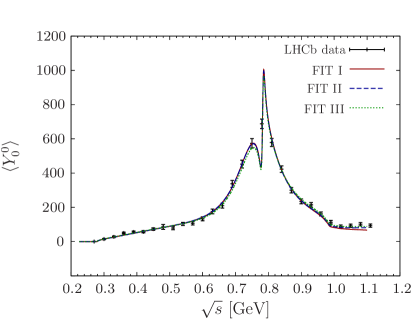
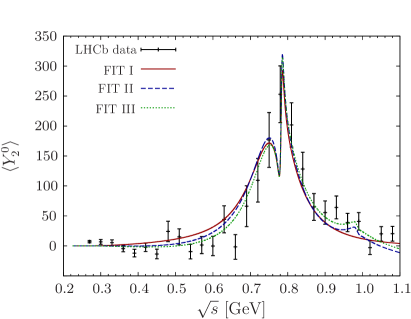
Figure 3: $\langle Y_{0}^{0}\rangle$ (left) simultaneously fitted with $\langle Y_{2}^{0}\rangle$ (right), using 3 parameters without $D$-wave contribution (FIT I, red, solid), and improving step by step by adding a Breit–Wigner-parametrized $D$-wave contribution (FIT II, blue, dashed) and by allowing for 4 free parameters, also supplemented by the $D$-wave contribution (FIT III, green, dotted).

	$\chi^{2}$/ndf	$|b_{0}^{n}|$	$|a_{0}|$	$|a_{\parallel}|$	$a^{\prime}_{0}$
FIT I	1.97	$10.3_{-1.8}^{+1.5}$	$46.5_{-6.8}^{+6.0}$	$51.8_{-11.0}^{+9.0}$	–
FIT II	1.54	$10.3_{-1.8}^{+1.5}$	$47.6_{-6.6}^{+5.8}$	$49.5_{-11.7}^{+9.4}$	–
FIT III	1.32	$10.6_{-1.8}^{+1.5}$	$37.7_{-21.3}^{+20.3}$	$48.2_{-12.4}^{+9.8}$	$0.4_{-0.7}^{+2.4}$

Table 1: Resulting fit parameters and $\chi^{2}$/ndf for the various fit configurations FIT I–III for the $\bar{B}_{d}^{0}\to J/\psi\pi^{+}\pi^{-}$ decay.

A key feature of the formalism employed here is its correct description of the $S$-wave. Figure 4 shows the comparison of the $S$-wave amplitude strength of the LHCb Breit–Wigner parametrization with the ones obtained in FIT I–III, as well as the comparison of the corresponding phases. In the elastic region, the phase of the non-strange scalar form factor $\delta_{\Gamma^{n}}=\text{arg}(\Gamma_{\pi}^{n})$ coincides with the $\pi\pi$ phase shift $\delta_{0}^{0}$ that we use as input for the Omnès matrix, in accordance with Watson’s theorem. Right above the $K\bar{K}$ threshold, $\delta_{\Gamma^{n}}$ drops quickly, which causes the dip in the region of the $f_{0}(980)$, visible in the modulus of the amplitudes as well as the non-Breit–Wigner bump structure in the $f_{0}(500)$ region. We find that the phase due to a Breit–Wigner parametrization largely differs from the dispersive solution, indicating that parametrizations of such kind are not well suited for studies of $CP$ violation in heavy-meson decays.

Note that in the analysis of Ref. Aaij:2014vda the $f_{0}(500)$ is modeled not by a Breit–Wigner function, but by the theoretically better motivated parametrization of Ref. Bugg:2006gc . In this work, higher resonances are included by multiplying $S$-matrix elements. While this procedure preserves unitarity, it produces terms at odds with any microscopic description of the coupled $\pi\pi$–$K\bar{K}$ system. As such also this approach introduces uncontrolled theoretical uncertainties into the analysis. The only stringently model-independent way to include hadronic final-state interactions is via dispersion theory.

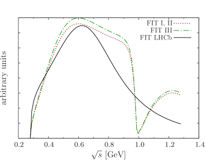
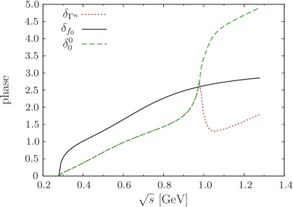
Figure 4: Comparison of the $S$-wave amplitude strength and phase obtained in the LHCb and in our fits, respectively. In the left panel the $S$-wave part of the decay rate for the three fit configurations FIT I–III is depicted together with the LHCb outcome. The right panel shows the phases of the non-strange scalar form factor $\delta_{\Gamma^{n}}$ (equal to the $\pi\pi$ $S$-wave phase shift $\delta_{0}^{0}$ below the $K\bar{K}$ threshold) compared to the $S$-wave phase $\delta_{f_{0}}$ extracted from the LHCb analysis.

4.2 $\bar{B}_{s}^{0}\to J/\psi\pi^{+}\pi^{-}$

The $\bar{B}_{s}^{0}\to J/\psi\pi^{+}\pi^{-}$ distribution in the region up to roughly 1  is clearly dominated by the $f_{0}(980)$. We therefore describe the data with the strange $S$-wave component only, using a constant subtraction polynomial ($c_{0}^{s}$). The only non-zero contribution to the fit thus comes from $\langle Y_{0}^{0}\rangle$. Fitting the data up to $\sqrt{s}=1.05~{}(1.02)~{}$ yields $\chi^{2}/{\rm ndf}=2.2~{}(1.8$) and $c_{0}^{s}=16.8\pm 0.4~{}(16.8\pm 0.4$). In analogy to the $\bar{B}_{d}^{0}$ decay we also perform the fit including the $D$-wave parametrization of the LHCb analysis. This yields an additional non-zero contribution to $\langle Y_{2}^{0}\rangle$ due to the $S$–$D$-wave interference, which is fitted simultaneously with $\langle Y_{0}^{0}\rangle$. Further, the influence of a linear subtraction polynomial for the strange $S$-wave is tested. However, none of these corrections exhibits a considerable improvement.

In the LHCb analysis the full energy range, $\sqrt{s}\leq 2.1~{}$, is fitted with 22 (24) parameters for Solution I (II). Confining to the region we examine in our fit and considering the $f_{0}(980)$ resonance only, the number of fit parameters reduces to four (six), and we calculate $\chi^{2}_{\rm LHCb}/{\rm ndf}=0.76\,(0.82)$, when using our definition of the $\chi^{2}$.

The strange scalar form factor, or the $f_{0}(980)$ peak in the dispersive formalism, depends crucially on the $\pi\pi\to K\bar{K}$ $S$-wave transition amplitude, which is not as accurately known as elastic $\pi\pi$ scattering (and even contains subtleties as non-negligible isospin breaking effects due to the different thresholds of charged and neutral kaons, see e.g. Ref. a0f0 ). As there are no error bands available for the Omnès matrix (or the various input quantities), to estimate the theoretical uncertainty we use and compare the fits resulting from the two different coupled-channel $T$-matrices described in Sec. 3. A minimization of the $\chi^{2}$ using the modified Omnès solution based on Ref. Dai:2014zta yields $\chi^{2}/{\rm ndf}=3.4~{}(2.4$) and $c_{0}^{s}=18.3\pm 0.5~{}(18.2\pm 0.5$). The resulting $\langle Y_{0}^{0}\rangle$ curves for both fits, using the phase input from the Bern CCL2012 ; CCLprep and Orsay BDM04 groups (B+O), as well the one of Ref. Dai:2014zta (DP), are presented in Fig. 5. Furthermore we show the phase shifts and the phases of the strange form factor for both phase inputs and compare to the LHCb phase due to Solution II (with $f_{0}(980)$ and a non-resonant $S$-wave contribution) as well as Solution I ($f_{0}(980)$ parametrization only). While the latter phase has a negative slope for $s\lesssim 1~{}$, which does not agree with the known phase shift, the phase extracted in Solution II is remarkably close to both the Bern and Madrid phase motions.

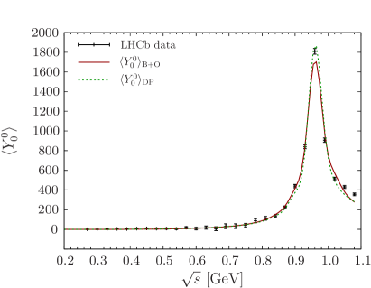
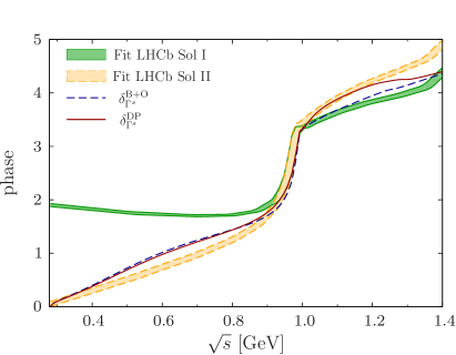
Figure 5: Left panel: $\langle Y_{0}^{0}\rangle$ fitted using the strange $S$-wave with constant subtraction polynomial for two different phase inputs (red, solid: B+O input CCL2012 ; CCLprep ; BDM04 , green, dotted: DP input Dai:2014zta , based on the Madrid–Kraków analysis GarciaMartin:2011cn ). Right panel: comparison of the phase of the strange scalar pion form factor for the B+O (blue, dashed) and DP (red, solid) input, respectively, with the $S$-wave phase extracted from the LHCb analysis (Solution I and II, shown with error bands).

4.3 $\bar{B}_{s}^{0}\to J/\psi K^{+}K^{-}$ $S$-wave prediction

Having obtained the $\bar{B}_{s}^{0}\to J/\psi\pi^{+}\pi^{-}$ fit parameters, we can make a prediction for the $\bar{B}_{s}^{0}\to J/\psi K^{+}K^{-}$ $S$-wave amplitudes, using the relation between the $\pi\pi$ and the $K\bar{K}$ final states provided by the coupled-channel formalism, cf. Appendix B.

In particular an understanding of the $S$-wave background to the prominent $\phi(1020)$ is of interest. In the LHCb analysis Aaij:2013orb , the $f_{0}(980)$ as well as a non-resonant $S$-wave content is reported within a mass window of $\pm 12$  around the $\phi(1020)$, which contribute an $S$-wave fraction of $(1.1\pm 0.1^{+0.2}_{-0.1})\%$—consistent with former measurements from LHCb, CDF, and ATLAS lhcbconf2012 ; Aaltonen:2012ie ; Aad:2012kba , as well as theoretical estimates Stone:2008ak . We calculate the $S$-wave fraction in the same mass interval $\pm 12$  around the $\phi(1020)$ mass adopting the LHCb Breit–Wigner parametrization for the $\phi(1020)$, but using the predicted $S$-wave for the $J/\psi K^{+}K^{-}$ final state. Naively, this $S$-wave can be obtained by replacing the pion scalar form factor and all pion masses and momenta by the respective kaon quantities and taking the resulting fit parameters from the pion case. However, the fit result depends on the normalization of the $\bar{B}_{s}^{0}\to J/\psi\pi^{+}\pi^{-}$ distribution. Hence, taking over the pion fit results for such a prediction requires a proper normalization of both decay channels relative to each other. To achieve this, we use the absolute branching fractions Agashe:2014kda

$$\mathcal{B}\left(\bar{B}_{s}^{0}\to J/\psi K^{+}K^{-}\right) = (7.9\pm 0.7)\times 10^{-4},$$

$$\mathcal{B}\left(\bar{B}_{s}^{0}\to J/\psi\pi^{+}\pi^{-}\right) = (2.12\pm 0.19)\times 10^{-4},$$

and define normalization constants

$$\mathcal{N}_{\{\pi,K\}}=\frac{\mathcal{B}(\bar{B}_{s}^{0}\to J/\psi\{\pi^{+}\pi^{-},K^{+}K^{-}\})}{N(\bar{B}_{s}^{0}\to J/\psi\{\pi^{+}\pi^{-},K^{+}K^{-}\})}\,,$$ (4.1)

where

$$N(\bar{B}_{s}^{0}\to J/\psi\{\pi^{+}\pi^{-},K^{+}K^{-}\})=\sqrt{4\pi}\int\left\langle Y_{0}^{0}\left(\bar{B}_{s}^{0}\to J/\psi\{\pi^{+}\pi^{-},K^{+}K^{-}\}\right)\right\rangle{\text{d}}\sqrt{s}$$ (4.2)

is the total number of events.

The $S$-wave contribution to the $\phi(1020)$ peak region is given by

$$\mathcal{R}_{S/\phi}\equiv\frac{\mathcal{N}_{\pi}\int_{m_{\phi}-12\,}^{m_{\phi}+12\,}X^{3}\sigma_{K}\sqrt{s}\left|c_{0}^{s}\Gamma_{K}^{s}(\sqrt{s})\right|^{2}\,{\text{d}}\sqrt{s}}{\ \int_{m_{\phi}-12\,}^{m_{\phi}+12\,}\sqrt{4\pi}\big{\langle}\tilde{Y}_{0}^{0}\left(\bar{B}_{s}^{0}\to J/\psi K^{+}K^{-}\right)\big{\rangle}\,{\text{d}}\sqrt{s}},$$ (4.3)

where we can approximate the (normalized) angular moment in the region of interest by the $S$-wave and the $\phi(1020)$ contribution,

$$\left.\sqrt{4\pi}\left\langle\tilde{Y}_{0}^{0}\left(\bar{B}_{s}^{0}\to J/\psi K^{+}K^{-}\right)\right\rangle\right|_{|\sqrt{s}-m_{\phi}|\lesssim 12~{}}$$

$$\qquad\qquad\approx X\sigma_{K}\sqrt{s}\bigg{(}X^{2}\mathcal{N}_{\pi}\left|c_{0}^{s}\Gamma_{K}^{s}(\sqrt{s})\right|^{2}+\mathcal{N}_{K}\sum_{\tau}\left|\alpha_{\tau}^{\phi}\mathcal{A}_{\phi}^{(\tau)}(s)\right|^{2}\bigg{)}.$$ (4.4)

Using the B+O input, we obtain $\mathcal{R}_{S/\phi}=1.1\%$, in agreement with the LHCb result. However, there is a notable uncertainty due to the estimated ambiguity in the phase input in the region of the $f_{0}(980)$ resonance discussed in Sec. 4.2. Using the DP phase instead of the B+O phase input yields a fraction of $1.95\%.$

5 Summary and outlook

In this article, we have described the strong-interaction part of the $\bar{B}_{d}^{0}\to J/\psi\pi^{+}\pi^{-}$ and $\bar{B}_{s}^{0}\to J/\psi\pi^{+}\pi^{-}$ decays by means of dispersively constructed scalar and vector pion form factors. This formalism respects all constraints from analyticity and unitarity. The non-strange and strange scalar form factors are calculated from a two-channel Muskhelishvili–Omnès formalism that requires the pion–pion elastic $S$-wave phase shift as well as modulus and phase of the corresponding $\pi\pi\to K\bar{K}$ amplitude as input. For the vector form factor, an elastic Omnès representation based solely on the pion–pion $P$-wave phase shift is sufficient, supplemented by an enhanced isospin-breaking contribution of $\rho$–$\omega$ mixing, which can be fixed from data on $e^{+}e^{-}\to\pi^{+}\pi^{-}$.

For energies $\sqrt{s}\leq 1.02~{}$, a minimal description of all $S$- and $P$-waves (constructed in a form free of kinematical singularities) as the corresponding form factors, multiplied by real constants, has been shown to be sufficient. Allowing for subtraction polynomials with linear $s$-dependence leads to a slightly improved fit quality solely in the case of one $P$-wave component, with a slope still compatible with zero within uncertainties. In particular considering the $S$-wave slope as a free fit parameter (as opposed to fixing it to zero) only yields a minimal improvement of the $\chi^{2}$. In accordance with expectations from the underlying tree-level decay mechanism, below the onset of $D$-wave contributions that become important with the $f_{2}(1270)$, only the non-strange scalar and the vector form factors feature in the $\bar{B}_{d}^{0}$ decay, while the strange scalar form factor determines the $\bar{B}_{s}^{0}$ $S$-wave.

The overall fit quality in the energy range considered is at least as good as in the phenomenological fits by the LHCb collaboration Aaij:2014siy ; Aaij:2014emv , where Breit–Wigner resonances and non-resonant background terms were used. However, since the dispersive analysis allows one to use input from other sources, our analysis calls for a much smaller number of parameters to be determined from the data. In addition, a comparison of the $\bar{B}_{d}^{0}$ $S$-wave obtained from the dispersive analysis with the one deduced from the LHCb analysis shows drastic differences in both modulus and phase: it is well-known that the $f_{0}(500)$ does not have a Breit–Wigner shape, and therefore such parametrizations should be avoided—especially when it comes to studies of $CP$ violation that need a reliable treatment of the phases induced by the hadronic final-state interactions Gardner:2001gc . The LHCb analysis of the $\bar{B}_{s}^{0}$ $S$-wave uses a Flatté parametrization of the $f_{0}(980)$, solely (corresponding to their Solution I) or combined with a non-resonant background (Solution II). Only Solution II yields a phase that is close to the phase of the strange scalar form factor, and approximately compatible with Watson’s final-state interaction theorem in the elastic region.

Finally we have made a prediction for the $\bar{B}_{s}^{0}\to J/\psi K^{+}K^{-}$ $S$-wave, which is related to the corresponding $\pi^{+}\pi^{-}$ final state through channel coupling. Only the results of the fit to the $\pi^{+}\pi^{-}$ final state are required to predict an $S$-wave fraction below the $\phi(1020)$ resonance of about 1.1%, in agreement with the findings by the LHCb collaboration. We have not attempted a corresponding prediction for the $\bar{B}_{d}^{0}\to J/\psi K^{+}K^{-}$ $S$-wave, since this has an isovector component (corresponding e.g. to the $a_{0}(980)$ resonance). This would have to be described by a coupled-channel treatment of the $\pi\eta$ and $K\bar{K}$ $S$-waves Albaladejo:2015aca .

To extend our description of the form factors to higher energies, eventually covering most of the energy range accessible in $\bar{B}_{d/s}^{0}\to J/\psi\pi^{+}\pi^{-}$, inelastic channels with corresponding higher resonances have to be taken into account. Here, a formalism recently developed for the vector form factor Hanhart:2012wi that correctly implements the analytic structure and unitarity, reduces to the Omnès representation in the elastic regime, but maps smoothly onto an isobar-model picture at higher energies should be extended to the scalar sector. Even an extraction of the scalar form factors from these high-precision LHCb data sets seems feasible, and should be pursued in the future.

Appendix A Form factors and partial-wave expansion

In the standard basis of momenta $p_{\psi}$, $P^{\mu}$, and $Q^{\mu}$, Eq. (2.4), the matrix element describing the hadronic part of the $\bar{B}_{d/s}^{0}$ decay is given by four dimensionless form factors, three axial ($\mathcal{A}_{i}$) and one vector ($\mathcal{V}$),

$$\mathcal{M}^{\pi\pi}_{\mu} =\langle\pi^{+}(p_{1})\pi^{-}(p_{2})|J_{\mu}^{d/s}|\bar{B}_{d/s}^{0}(p_{B})\rangle=P_{\mu}\mathcal{A}_{1}+Q_{\mu}\mathcal{A}_{2}+(p_{\psi})_{\mu}\mathcal{A}_{3}+i\epsilon_{\mu\nu\rho\sigma}p_{\psi}^{\nu}P^{\rho}Q^{\sigma}\mathcal{V},$$

$$J_{\mu}^{q} =\bar{q}\gamma_{\mu}(1-\gamma_{5})b.$$ (A.1)

In Sec. 2.2 we use a different (orthogonal) basis of momentum vectors, $p_{\psi}^{\mu}$, $\bar{p}_{(\perp)}^{\mu}$, and $Q_{(\parallel)}^{\mu}$, see Eq. (2.8), corresponding to the orthonormal basis of polarization vectors of the $J/\psi$ meson Faller:2013dwa ,

$$\epsilon^{\mu}(t)=\frac{p_{\psi}^{\mu}}{M_{\psi}},\quad\epsilon^{\mu}(0)=-\frac{M_{\psi}}{X}P^{\mu}_{(0)},\quad\epsilon^{\mu}(\pm)=-\frac{1}{\sqrt{2s}\,\sigma_{\pi}\sin\theta_{\pi}}\left(Q_{(\parallel)}^{\mu}\mp i\bar{p}_{(\perp)}^{\mu}\right)e^{\mp i\phi}.$$ (A.2)

This allows us to describe the matrix element $\mathcal{M}_{\pi\pi}^{\mu}$ in terms of the transversity form factors, Eq. (2.2), or similarly (with regard to an easily performable partial-wave expansion) in terms of helicity form factors, defined via the contraction of $\mathcal{M}_{\pi\pi}^{\mu}$ with the polarization vector,

$$\mathcal{H}_{\lambda}=\langle\pi^{+}\pi^{-}|J_{\mu}^{d/s}|\bar{B}_{d/s}^{0}\rangle\,\epsilon_{\mu}^{\dagger}(\lambda).$$ (A.3)

The relations between the transversity and helicity form factors can be read off to be

$$\mathcal{H}_{t}=\mathcal{F}_{t},\quad\mathcal{H}_{0}=\mathcal{F}_{0},\quad\mathcal{H}_{\pm}=(\mathcal{F}_{\parallel}\pm\mathcal{F}_{\perp})\frac{\sigma_{\pi}}{\sqrt{2}}\sin\theta_{\pi}e^{\pm i\phi},$$ (A.4)

as well as those to the set {$\mathcal{A}_{i},\,\mathcal{V}$},

$$\mathcal{F}_{\perp} = -\sqrt{s}X\mathcal{V},\quad\mathcal{F}_{\parallel}=\sqrt{s}\mathcal{A}_{2},\quad\mathcal{F}_{0}=\frac{X}{2M_{\psi}}\left(2\mathcal{A}_{1}+\frac{\sigma_{\pi}\cos\theta_{\pi}(P\cdot p_{\psi})}{X}\mathcal{A}_{2}\right),$$

$$\mathcal{F}_{t} = \frac{P\cdot Q}{M_{\psi}}\mathcal{A}_{1}+\frac{\sigma_{\pi}X\cos\theta_{\pi}}{2XM_{\psi}}\left((P\cdot p_{\psi})(P\cdot Q)-sM_{\psi}^{2}\right)\mathcal{A}_{2}+M_{\psi}\mathcal{A}_{3}.$$ (A.5)

The unphysical time component $\mathcal{F}_{t}$ does not contribute. We expand the remaining three form factors $\mathcal{H}_{0,\pm}$ in partial waves. The latter relation is of particular interest when defining partial waves that are free of kinematical singularities and zeros, see Sec. 3.

The partial-wave expansion of the helicity amplitudes reads

$$\mathcal{H}_{\lambda}(s)=\sum_{\ell}\sqrt{2\ell+1}\mathcal{H}_{\lambda}^{(\ell)}(s)d_{\lambda 0}^{\ell}(\theta_{\pi})e^{\lambda i\phi},$$ (A.6)

where the $d_{\lambda\lambda^{\prime}}^{\ell}$ are the small Wigner-$d$ functions. Using

$$d_{00}^{\ell}(\theta_{\pi})=P_{\ell}(\cos\theta_{\pi}),\quad d_{10}^{\ell}(\theta_{\pi})=-d_{-10}^{\ell}(\theta_{\pi})=-\frac{\sin\theta_{\pi}}{\sqrt{\ell(\ell+1)}}P_{\ell}^{\prime}(\cos\theta_{\pi}),$$ (A.7)

we see that the zero-component $\mathcal{H}_{0}(s)$ is expanded in terms of Legendre polynomials $P_{\ell}(\cos\theta_{\pi})$ and thus contains all $S$-, $P$-, and $D$-wave contributions, while the $\mathcal{H}_{\pm}(s)$ partial-wave expansions, proceeding in derivatives of the Legendre polynomials $P_{\ell}^{\prime}(\cos\theta_{\pi})$, start with the $P$-wave amplitudes, i.e.

$$\mathcal{H}_{0}(s) = \mathcal{H}_{0}^{(S)}(s)+\sqrt{3}\cos\theta_{\pi}\mathcal{H}_{0}^{(P)}(s)+\frac{\sqrt{5}}{2}\left(3\cos^{2}\theta_{\pi}-1\right)\mathcal{H}_{0}^{(D)}(s)+\dots\,,$$

$$\mathcal{H}_{\pm}(s) = \mp\sqrt{\frac{3}{2}}\sin\theta_{\pi}\left(\mathcal{H}_{\pm}^{(P)}(s)+\sqrt{5}\cos\theta_{\pi}\mathcal{H}_{\pm}^{(D)}(s)\right)e^{\pm i\phi}+\dots,$$ (A.8)

where the ellipses denote $F$-waves and larger. Equivalently, due to Eq. (A.4) and using $\mathcal{H}_{\pm}^{(\ell)}(s)=\mp\frac{\sigma_{\pi}}{\sqrt{2}}\big{(}\mathcal{F}_{\parallel}^{(\ell)}(s)\pm\mathcal{F}_{\perp}^{(\ell)}(s)\big{)}$, we arrive at the partial-wave expansion of the transversity form factors given in Eq. (2.9) in the main text.

In order to calculate the differential decay rate we sum over the squared helicity amplitudes,

$$\left|\overline{\mathcal{M}}\right|^{2}=\frac{G_{F}^{2}}{2}|V_{cb}|^{2}|V_{cq}|^{2}f_{\psi}^{2}M_{\psi}^{2}\left(|\mathcal{H}_{0}|^{2}+|\mathcal{H}_{+}|^{2}+|\mathcal{H}_{-}|^{2}\right)\quad(q=\{d,s\})$$ (A.9)

and integrate over the invariant three-particle phase space, which is given by

$${\text{d}}\Phi^{(3)}=\frac{X\sigma_{\pi}}{4(4\pi)^{2}m_{B}^{2}}\,{\text{d}}s\,{\text{d}}\cos\theta_{\pi}\,{\text{d}}\phi.$$ (A.10)

Neglecting waves larger than $D$-waves and integrating over $\phi$ we arrive at Eq. (2.11).

Appendix B Coupled-channel Omnès formalism

We briefly discuss the coupled-channel derivation of the scalar pion and kaon form factors ($I=0,\ell=0$). The two-channel unitarity relation reads

$$\mbox{disc}\,\mathbf{\Gamma}(s)=2iT^{0*}_{0}(s)\Sigma(s)\mathbf{\Gamma}(s),$$ (B.1)

where the two-dimensional vector $\mathbf{\Gamma}(s)$ contains the pion and kaon scalar isoscalar form factors and $T^{0}_{0}(s)$ and $\Sigma(s)$ are two-dimensional matrices,

$$T^{0}_{0}(s)=\left(\begin{array}[]{cc}\dfrac{\eta^{0}_{0}(s)e^{2i\delta^{0}_{0}(s)}-1}{2i{\sigma}_{\pi}(s)}&|g^{0}_{0}(s)|e^{i\psi^{0}_{0}(s)}\\[6.0pt] |g^{0}_{0}(s)|e^{i\psi^{0}_{0}(s)}&\dfrac{\eta^{0}_{0}(s)e^{2i(\psi^{0}_{0}(s)-\delta^{0}_{0}(s))}-1}{2i{\sigma}_{K}(s)}\end{array}\right),$$ (B.2)

and $\Sigma(s)=\mbox{diag}\left(\sigma_{\pi}(s)\Theta(s-4M_{\pi}^{2}),\sigma_{K}(s)\Theta(s-4M_{K}^{2})\right)$, with $\sigma_{i}(s)=\left(1-4M_{i}^{2}/s\right)^{1/2}$ and $\Theta(.)$ denoting the Heaviside function. There are three input functions entering the $T$-matrix, the $\pi\pi$ $S$-wave isoscalar phase shift $\delta^{0}_{0}(s)$ and the $\pi\pi\to K\bar{K}$ $S$-wave amplitude $g^{0}_{0}(s)=|g^{0}_{0}(s)|{\rm exp}(i\psi^{0}_{0}(s))$ with modulus and phase. The modulus $|g^{0}_{0}(s)|$ is related to the inelasticity parameter $\eta^{0}_{0}(s)$ by

$$\eta^{0}_{0}(s)=\sqrt{1-4\sigma_{\pi}(s)\sigma_{K}(s)|g^{0}_{0}(s)|^{2}\Theta(s-4M_{K}^{2})}.$$ (B.3)

Writing the two-dimensional dispersion integral over the discontinuity (B.1) leads to a system of coupled Muskhelishvili–Omnès equations,

$$\mathbf{\Gamma}(s)=\frac{1}{\pi}\int_{4M_{\pi}^{2}}^{\infty}\frac{T^{0*}_{0}(s^{\prime})\Sigma(s^{\prime})\mathbf{\Gamma}(s^{\prime})}{s^{\prime}-s-i\epsilon}{\text{d}}s^{\prime}.$$ (B.4)

A solution can be constructed introducing a two-dimensional Omnès matrix, which is connected to the form factors by means of a multiplication with a vector containing the normalizations $\Gamma_{\pi}(0)$ and $\Gamma_{K}(0)$ DGL90 ,

$$\left(\begin{array}[]{c}\Gamma_{\pi}(s)\\ \smash{\frac{2}{\sqrt{3}}}\Gamma_{K}(s)\end{array}\right)=\left(\begin{array}[]{cc}\Omega_{11}(s)&\Omega_{12}(s)\\ \Omega_{21}(s)&\Omega_{22}(s)\end{array}\right)\left(\begin{array}[]{c}\Gamma_{\pi}(0)\\ \smash{\frac{2}{\sqrt{3}}}\Gamma_{K}(0)\end{array}\right),$$ (B.5)

where $\Gamma_{\pi,K}(s)$ represents both strange and non-strange form factors, $\Gamma^{s}_{\pi,K}(s)$ and $\Gamma^{n}_{\pi,K}(s)$, which differ merely in their respective normalizations. Thus the problem reduces to finding a matrix $\Omega(s)$ that fulfills

$$\text{Im}\,\,\Omega(s)=T^{0*}_{0}(s)\Sigma(s)\Omega(s),\quad\Omega(s)=\frac{1}{\pi}\int_{4M_{\pi}^{2}}^{\infty}\frac{T^{0*}_{0}(s^{\prime})\Sigma(s^{\prime})\Omega(s^{\prime})}{s^{\prime}-s-i\epsilon}{\text{d}}s^{\prime},\quad\Omega(0)=\mathbbm{1},$$ (B.6)

which has to be solved numerically DGL90 ; Moussallam2000 ; Sebastien ; Hoferichter:2012wf . To ensure an adequate asymptotic behavior, we exploit the correlation between the high-energy behavior of the Omnès solution and the sum of the eigen phase shifts $\sum\delta_{\ell}^{I}(s)$ Moussallam2000 ,

$$\sum\delta_{\ell}^{I}(s)\overset{s\to\infty}{\longrightarrow}\,m\pi=\left\{\begin{array}[]{cc}\pi\quad\;\,{\rm for}\quad I=1,~{}\ell=1\\ 2\pi\quad{\rm for}\quad I=0,~{}\ell=0\end{array}\right.\quad\quad\Longleftrightarrow\quad\Omega_{\ell}^{I}(s)\overset{s\to\infty}{\longrightarrow}\,\frac{1}{s}\,,$$ (B.7)

where $m$ is the number of channels that are treated in the formalism.

According to the Feynman–Hellmann theorem, the form factors for zero momentum are related to the corresponding Goldstone boson masses, which at next-to-leading order in the chiral expansion in terms of quark masses depend on certain low-energy constants. These are determined in lattice simulations with $N_{f}=2+1$ dynamical flavors at a running scale $\mu=\mathrm{770}{}$ Aoki:2013ldr , limiting the form factor normalizations to the ranges

$$\Gamma_{\pi}^{n}(0) =0.984\pm 0.006, \Gamma_{\pi}^{s}(0) =(-0.001\dots 0.006)\approx 0,$$

$$\Gamma_{K}^{n}(0) =(0.4\dots 0.6), \Gamma_{K}^{s}(0) =(0.95\dots 1.15).$$ (B.8)

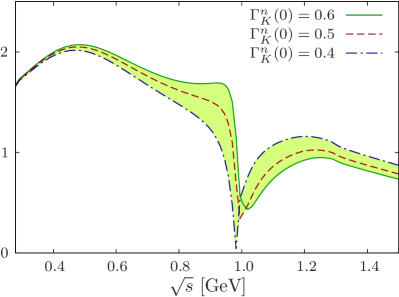
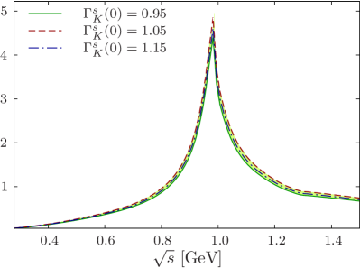
Figure 6: Modulus of the scalar pion non-strange (left panel) and strange (right panel) form factors, depicted for three different normalizations inside the allowed range, illustrated by the uncertainty band.

Figure 6 shows the results obtained for the modulus of the pion form factor (see also Ref. Daub:2012mu ). The sensitivity due to the uncertainty in the kaon form factor normalization is illustrated by the uncertainty bands. The strange form factor exhibits a peak around $1~{}$, which is produced by the $f_{0}(980)$ resonance. On the contrary in the pion non-strange form factor the $\sigma$ meson appears as a broad bump (notice the non-Breit–Wigner shape) around 500 .

References

- (1) M. Battaglieri et al., Acta Phys. Polon. B 46 (2015) 257 [arXiv:1412.6393 [hep-ph]].
- (2) J. Dalseno et al. [Belle Collaboration], Phys. Rev. D 79 (2009) 072004 [arXiv:0811.3665 [hep-ex]].
- (3) B. Aubert et al. [BaBar Collaboration], Phys. Rev. D 80 (2009) 112001 [arXiv:0905.3615 [hep-ex]].
- (4) Y. Nakahama et al. [Belle Collaboration], Phys. Rev. D 82 (2010) 073011 [arXiv:1007.3848 [hep-ex]].
- (5) J. P. Lees et al. [BaBar Collaboration], Phys. Rev. D 85 (2012) 112010 [arXiv:1201.5897 [hep-ex]].
- (6) R. Aaij et al. [LHCb Collaboration], Phys. Rev. D 90 (2014) 012003 [arXiv:1404.5673 [hep-ex]].
- (7) R. Aaij et al. [LHCb Collaboration], Phys. Rev. D 89 (2014) 092006 [arXiv:1402.6248 [hep-ex]].
- (8) B. Aubert et al. [BaBar Collaboration], Phys. Rev. Lett. 90 (2003) 091801 [hep-ex/0209013].
- (9) J. Li et al. [Belle Collaboration], Phys. Rev. Lett. 106 (2011) 121802 [arXiv:1102.2759 [hep-ex]].
- (10) T. Aaltonen et al. [CDF Collaboration], Phys. Rev. D 84 (2011) 052012 [arXiv:1106.3682 [hep-ex]].
- (11) V. M. Abazov et al. [D0 Collaboration], Phys. Rev. D 85 (2012) 011103 [arXiv:1110.4272 [hep-ex]].
- (12) R. Aaij et al. [LHCb Collaboration], Phys. Rev. D 87 (2013) 052001 [arXiv:1301.5347 [hep-ex]].
- (13) R. Aaij et al. [LHCb Collaboration], Phys. Rev. D 86 (2012) 052006 [arXiv:1204.5643 [hep-ex]].
- (14) S. Gardner and U.-G. Meißner, Phys. Rev. D 65 (2002) 094004 [hep-ph/0112281].
- (15) W. H. Liang and E. Oset, Phys. Lett. B 737 (2014) 70 [arXiv:1406.7228 [hep-ph]].
- (16) U.-G. Meißner and J. A. Oller, Nucl. Phys. A 679 (2001) 671 [hep-ph/0005253].
- (17) T. A. Lähde and U.-G. Meißner, Phys. Rev. D 74 (2006) 034021 [hep-ph/0606133].
- (18) B. Ananthanarayan, G. Colangelo, J. Gasser and H. Leutwyler, Phys. Rept. 353 (2001) 207 [hep-ph/0005297].
- (19) R. García-Martín, R. Kamiński, J. R. Peláez, J. Ruiz de Elvira and F. J. Ynduráin, Phys. Rev. D 83 (2011) 074004 [arXiv:1102.2183 [hep-ph]].
- (20) I. Caprini, G. Colangelo and H. Leutwyler, Eur. Phys. J. C 72 (2012) 1860 [arXiv:1111.7160 [hep-ph]];
- (21) I. Caprini, G. Colangelo and H. Leutwyler, in preparation.
- (22) P. Büttiker, S. Descotes-Genon, and B. Moussallam, Eur. Phys. J. C 33 (2004) 409 [arXiv:0310283 [hep-ph]].
- (23) M. Bayar, W. H. Liang and E. Oset, Phys. Rev. D 90 (2014) 114004 [arXiv:1408.6920 [hep-ph]].
- (24) J. J. Xie and E. Oset, Phys. Rev. D 90 (2014) 094006 [arXiv:1409.1341 [hep-ph]].
- (25) S. Stone and L. Zhang, Phys. Rev. Lett. 111 (2013) 062001 [arXiv:1305.6554 [hep-ex]].
- (26) P. Colangelo, F. De Fazio and W. Wang, Phys. Rev. D 81 (2010) 074001 [arXiv:1002.2880 [hep-ph]].
- (27) W. F. Wang, H. n. Li, W. Wang and C.-D. Lü, Phys. Rev. D 91 (2015) 094024 [arXiv:1502.05483 [hep-ph]].
- (28) S. Faller, T. Feldmann, A. Khodjamirian, T. Mannel and D. van Dyk, Phys. Rev. D 89 (2014) 014015 [arXiv:1310.6660 [hep-ph]].
- (29) G. Buchalla, A. J. Buras and M. E. Lautenbacher, Rev. Mod. Phys. 68 (1996) 1125 [hep-ph/9512380].
- (30) L. Liu, H. W. Lin and K. Orginos, PoS LATTICE 2008 (2008) 112 [arXiv:0810.5412 [hep-lat]].
- (31) M. Beneke, G. Buchalla, M. Neubert and C. T. Sachrajda, Nucl. Phys. B 591 (2000) 313 [hep-ph/0006124].
- (32) M. Diehl and G. Hiller, JHEP 0106 (2001) 067 [hep-ph/0105194].
- (33) R. Aaij et al. [LHCb Collaboration], Phys. Lett. B 742 (2015) 38 [arXiv:1411.1634 [hep-ex]].
- (34) P. Frings, U. Nierste and M. Wiebusch, Phys. Rev. Lett. 115 (2015) 061802 [arXiv:1503.00859 [hep-ph]].
- (35) P. Colangelo, F. De Fazio and W. Wang, Phys. Rev. D 83 (2011) 094027 [arXiv:1009.4612 [hep-ph]].
- (36) K. M. Watson, Phys. Rev. 95 (1954) 228.
- (37) M. F. Heyn and C. B. Lang, Z. Phys. C 7 (1981) 169.
- (38) R. Omnès, Nuovo Cim. 8 (1958) 316.
- (39) C. Hanhart, A. Kupść, U.-G. Meißner, F. Stollenwerk and A. Wirzba, Eur. Phys. J. C 73 (2013) 2668 [Eur. Phys. J. C 75 (2015) 242] [arXiv:1307.5654 [hep-ph]].
- (40) B. Aubert et al. [BaBar Collaboration], Phys. Rev. Lett. 103 (2009) 231801 [arXiv:0908.3589 [hep-ex]].
- (41) F. Ambrosino et al. [KLOE Collaboration], Phys. Lett. B 700 (2011) 102 [arXiv:1006.5313 [hep-ex]].
- (42) M. Ablikim et al. [BESIII Collaboration], Phys. Lett. B 753 (2016) 629 [arXiv:1507.08188 [hep-ex]].
- (43) S. Gardner and H. B. O’Connell, Phys. Rev. D 57 (1998) 2716 [Phys. Rev. D 62 (2000) 019903] [hep-ph/9707385].
- (44) H. Leutwyler, hep-ph/0212324.
- (45) C. Hanhart, Phys. Lett. B 715 (2012) 170 [arXiv:1203.6839 [hep-ph]].
- (46) S. Gardner, H. B. O’Connell and A. W. Thomas, Phys. Rev. Lett. 80 (1998) 1834 [hep-ph/9705453].
- (47) B. Ananthanarayan, I. Caprini, G. Colangelo, J. Gasser and H. Leutwyler, Phys. Lett. B 602 (2004) 218 [hep-ph/0409222].
- (48) D. H. Cohen et al., Phys. Rev. D 22 (1980) 2595.
- (49) A. Etkin et al., Phys. Rev. D 25 (1982) 1786.
- (50) L. Y. Dai and M. R. Pennington, Phys. Rev. D 90 (2014) 036004 [arXiv:1404.7524 [hep-ph]].
- (51) B. Hyams et al., Nucl. Phys. B 64 (1973) 134.
- (52) G. Grayer et al., Nucl. Phys. B 75 (1974) 189.
- (53) B. Hyams et al., Nucl. Phys. B 100 (1975) 205.
- (54) J. R. Batley et al. [NA48/2 Collaboration], Eur. Phys. J. C 54 (2008) 411.
- (55) J. R. Batley et al. [NA48/2 Collaboration], Eur. Phys. J. C 70 (2010) 635.
- (56) B. Aubert et al. [BaBar Collaboration], Phys. Rev. D 79 (2009) 032003 [arXiv:0808.0971 [hep-ex]].
- (57) P. del Amo Sanchez et al. [BaBar Collaboration], Phys. Rev. D 83 (2011) 052001 [arXiv:1011.4190 [hep-ex]].
- (58) K. A. Olive et al. [Particle Data Group Collaboration], Chin. Phys. C 38 (2014) 090001.
- (59) D. V. Bugg, J. Phys. G 34 (2007) 151 [hep-ph/0608081].
- (60) C. Hanhart, B. Kubis and J. R. Peláez, Phys. Rev. D 76 (2007) 074028 [arXiv:0707.0262 [hep-ph]].
- (61) R. Aaij et al. [LHCb Collaboration], Phys. Rev. D 88 (2013) 072005 [arXiv:1308.5916 [hep-ex]].
- (62) R. Aaij et al. [LHCb Collaboration], Phys. Rev. D 87 (2013) 072004 [arXiv:1302.1213 [hep-ex]].
- (63) R. Aaij et al. [LHCb Collaboration], LHCb-CONF-2012-002.
- (64) T. Aaltonen et al. [CDF Collaboration], Phys. Rev. Lett. 109 (2012) 171802 [arXiv:1208.2967 [hep-ex]].
- (65) G. Aad et al. [ATLAS Collaboration], JHEP 1212 (2012) 072 [arXiv:1208.0572 [hep-ex]].
- (66) S. Stone and L. Zhang, Phys. Rev. D 79 (2009) 074024 [arXiv:0812.2832 [hep-ph]].
- (67) M. Albaladejo and B. Moussallam, Eur. Phys. J. C 75 (2015) 488 [arXiv:1507.04526 [hep-ph]].
- (68) J. F. Donoghue, J. Gasser and H. Leutwyler, Nucl. Phys. B 343 (1990) 341.
- (69) B. Moussallam, Eur. Phys. J. C 14 (2000) 111 [arXiv:9909292 [hep-ph]].
- (70) S. Descotes-Genon, Ph.D. Thesis, Université de Paris-Sud, France (2000).
- (71) M. Hoferichter, C. Ditsche, B. Kubis and U.-G. Meißner, JHEP 1206 (2012) 063 [arXiv:1204.6251 [hep-ph]].
- (72) S. Aoki et al., Eur. Phys. J. C 74 (2014) 2890 [arXiv:1310.8555 [hep-lat]].
- (73) R. J. Dowdall, C. T. H. Davies, G. P. Lepage and C. McNeile, Phys. Rev. D 88 (2013) 074504 [arXiv:1303.1670 [hep-lat]].
- (74) J. T. Daub, H. K. Dreiner, C. Hanhart, B. Kubis and U.-G. Meißner, JHEP 1301 (2013) 179 [arXiv:1212.4408 [hep-ph]].