Towards an $H$-theorem for granular gases

Abstract

The $H$-theorem, originally derived at the level of Boltzmann non-linear kinetic equation for a dilute gas undergoing elastic collisions, strongly constrains the velocity distribution of the gas to evolve irreversibly towards equilibrium. As such, the theorem could not be generalized to account for dissipative systems: the conservative nature of collisions is an essential ingredient in the standard derivation. For a dissipative gas of grains, we construct here a simple functional $\mathscr{H}$ related to the original $H$, that can be qualified as a Lyapunov functional. It is positive, and results backed by three independent simulation approaches (a deterministic spectral method, the stochastic Direct Simulation Monte Carlo technique, and Molecular Dynamics) indicate that it is also non-increasing. Both driven and unforced cases are investigated.

I Introduction

In 1872, Boltzmann published one of his most important papers Boltzmann . This contribution can arguably be considered as the effective birth of kinetic theory, a domain pioneered by Bernoulli, Joule and Maxwell to name but a few, and that has turned into an active field of research in mathematics Villani02 , physics Cercignani , and engineering Bellomo . The interest of reference Boltzmann is twofold. First, the time evolution of the velocity distribution function $f(\mathbf{v},t)$ for a dilute gas far from equilibrium was derived, under the essential assumption of molecular chaos (Stosszahlansatz), that is, assuming the absence of correlations between the pre-collisional velocities of colliding partners Boltzmann2 ; Cercignani_book . For the sake of the discussion, we omit here the spatial dependence of the velocity distribution. Second and remarkably, Boltzmann also introduced a functional $H(t)=\int f\log f\,{\rm d}\mathbf{v}$ of the instantaneous and time dependent distribution function $f$, that can be seen as a non-equilibrium entropy: the corresponding $H$-theorem Boltzmann2 ; Cercignani_book states that this functional has a negative production, and vanishes only in equilibrium rque1 ; rque2 . It therefore is a Lyapunov-like functional. This explains in this particular context how molecular collisions irreversibly lead to equilibrium. Given that the underlying equations of motion are time-reversible (with elastic collisions), this finding ignited a long lasting and heated debate, an account of which is not the purpose of the present paper, and can be found in Brush ; Cercignani98 (see also Lebowitz and references therein for a more technical discussion). In essence, the statistical nature of the $H$-theorem was not fully recognized in the early days. Ironically, when dissipative collisions are considered –as e.g. is the case between macroscopic grains for which the equations of motion are irreversible g03 ; BP –, a well defined time’s arrow is present at the level of interactions, but no $H$-like theorem could be derived so far Villani06 ; Bena .

The aim of this paper is to present strong hints that a simple generalization of Boltzmann’s original functional can be constructed, that exhibits monotonous behavior with time and tends to zero. More specifically, we shall be interested in the dynamical behavior of a spatially homogeneous granular gas, made up of a collection of a large number of grains undergoing dissipative collisions. The grains are treated as inelastic hard spheres, see e.g g03 ; barrat05 for reviews of the rich phenomenology of this class of systems. We will consider two cases depending on the dynamics of the grains between collisions: the free-cooling case on the one hand, in which the grains move freely and the stochastic thermostat case on the other hand, in which the grains are driven by some random external force. In the first case, it is known from particle simulations that the system reaches an auto-similar regime in which all the time dependence in the one-particle distribution function goes through the instantaneous temperature (defined as the second velocity moment of the distribution) GoSh95 ; MiM1 ; BoCe . In the second case, a stationary state is reached in which the energy lost in collisions is compensated by the energy injected by the thermostat MiM2 .

We first study an $N$-particle model where the dynamics of the particles’ velocities are treated as a Markov process. A Lyapunov function can be identified exactly implying, under plausible conditions, that the thermostated system reaches the stationary state in the long-time limit. In the free-cooling case, the consequence is that all the time dependence in the $N$-particle probability distribution is encoded in the instantaneous temperature. This scaling is similar to the one proposed in BDS97 at the level of the Liouville equation and, of course, implies the one at the level of the one-particle distribution. Inspired by the previous model, we propose a Lyapunov functional for the inelastic homogeneous non-linear Boltzmann equation that describe the dynamics of the system in the low density limit and for $N\to\infty$ BDS97 ; BP . The functional is measured in three independent and complementary numerical techniques, with the result that it is always a nonincreasing function of time. These results point in the same direction as those of mpv13 , which focussed on thermostatted systems with emphasis on simplified collision models or kernel.

The structure of the paper is the following. In section II, the $N$-particle model is introduced and the corresponding $H$-functional identified. This is then analyzed in section III at the level of the one-particle distribution function to in turn define, in section IV, the candidate Lyapunov function that is a central object in our work. In section IV, simulation results are also shown. Finally, the last section contains some summarizing remarks.

II $N$-particle description

We consider a system of $N$ inelastic particles of mass $m$, diameter $\sigma$ and spatial dimension $d$. We will assume that a microstate is specified by giving the velocities of the $N$ particles, $\mathbf{V}(t)\equiv\{\mathbf{v}_{i}(t)\}_{i=1}^{N}$, at a given time $t$. The dynamics is Markovian, generated by the following rule: two particles $i$ and $j$ are chosen at random, together with a unit, center-to-center vector $\boldsymbol{\hat{\sigma}}$, from which the postcollisinal velocities $\mathbf{v}_{i}^{\prime},\mathbf{v}_{j}^{\prime}$ follow

$$\mathbf{v}_{i}^{\prime} = \mathbf{v}_{i}-\frac{1+\alpha}{2}(\boldsymbol{\hat{\sigma}}\cdot\mathbf{v}_{ij})\boldsymbol{\hat{\sigma}},$$ (1)

$$\mathbf{v}_{j}^{\prime} = \mathbf{v}_{j}+\frac{1+\alpha}{2}(\boldsymbol{\hat{\sigma}}\cdot\mathbf{v}_{ij})\boldsymbol{\hat{\sigma}}.$$ (2)

Here, $\mathbf{v}_{ij}=\mathbf{v}_{i}-\mathbf{v}_{j}$, and $\alpha$ is the coefficient of normal restitution that will be considered velocity-independent. It fulfills $0<\alpha\leq 1$ and collisions are elastic for $\alpha=1$. In the hard particle model, the collision frequency is proportional to $(\boldsymbol{\hat{\sigma}}\cdot\mathbf{v}_{ij})$. Nevertheless, we will consider a more general model in which this frequency is proportional to $(\boldsymbol{\hat{\sigma}}\cdot\mathbf{v}_{ij})^{\gamma}$ where $\gamma$ is a fixed positive parameter ($\gamma\geq 0$) ErTB06 . Then, the hard particles model is obtained for $\gamma=1$, while Maxwell molecules are for $\gamma=0$. Two cases shall be considered, depending on the dynamics of the grains between collisions.

II.1 The unforced system

Let us first address the free-cooling case. With the dynamics specified above, trajectories are generated and the state of the system is described in terms of the $N$-particle distribution function, $\rho_{N}(\mathbf{V},t)$. The evolution equation for this distribution is the generalization for inelastic collisions of the Kac’s equation Kac

$$\frac{\partial}{\partial t}\rho_{N}(\mathbf{V},t)=\frac{K}{N}\sum_{i<j}L(\mathbf{v}_{i},\mathbf{v}_{j})\rho_{N}(\mathbf{V},t),$$ (3)

where we have introduced the operator

$$L(\mathbf{v}_{i},\mathbf{v}_{j})\rho_{N}(\mathbf{V})=\int(\boldsymbol{\hat{\sigma}}\cdot\mathbf{v}_{ij})^{\gamma}\left[\frac{1}{\alpha^{\gamma+1}}b_{\boldsymbol{\hat{\sigma}}}(i,j)^{-1}-1\right]\rho_{N}(\mathbf{V},t)\,{\rm d}\boldsymbol{\hat{\sigma}},$$ (4)

and $K$ is a parameter of the model with the only restriction that $K(\boldsymbol{\hat{\sigma}}\cdot\mathbf{v}_{ij})^{\gamma}$ has dimensions of inverse of time (in the hard sphere case it is $K=n\sigma^{d-1}$, where $n$ is the density). The operator $b_{\boldsymbol{\hat{\sigma}}}(i,j)^{-1}$ acts on any function of $\mathbf{V}$ replacing $\mathbf{v}_{i}$ and $\mathbf{v}_{j}$ by the precollisional velocities, i.e.

$$b_{\boldsymbol{\hat{\sigma}}}(i,j)^{-1}f(\mathbf{V})=f(\mathbf{v}_{1},\dots,\mathbf{v}_{i-1},\mathbf{v}_{i}^{*},\mathbf{v}_{i+1},\dots,\mathbf{v}_{j-1},\mathbf{v}_{j}^{*},\mathbf{v}_{j+1},\dots,\mathbf{v}_{N}),$$ (5)

found from inverting the law (1)-(2)

$$\mathbf{v}_{i}^{*} = \mathbf{v}_{i}-\frac{1+\alpha}{2\alpha}(\boldsymbol{\hat{\sigma}}\cdot\mathbf{v}_{ij})\boldsymbol{\hat{\sigma}},$$ (6)

$$\mathbf{v}_{j}^{*} = \mathbf{v}_{j}+\frac{1+\alpha}{2\alpha}(\boldsymbol{\hat{\sigma}}\cdot\mathbf{v}_{ij})\boldsymbol{\hat{\sigma}}.$$ (7)

It can be seen that Eq. (3) admits a special solution in which all the time dependence in the distribution function is subsumed in the granular temperature, $T(t)$, defined as

$$\frac{d}{2}NT(t)=\int\,{\rm d}\mathbf{v}\frac{m}{2}\sum_{i=1}^{N}v_{i}^{2}\rho_{N}(\mathbf{V},t).$$ (8)

By dimensional analysis, this means that

$$\rho_{N}(\mathbf{V},t)=\frac{1}{v_{H}(t)^{dN}}\varphi_{N}\left[\frac{\mathbf{V}}{v_{H}(t)}\right],$$ (9)

where $v_{H}(t)\equiv\left[\frac{2T(t)}{m}\right]^{1/2}$ is the thermal velocity. In Appendix A, a consistent equation for $\varphi_{N}$ is obtained and the equation for the temperature is analyzed. For $\gamma>0$, the temperature behaves for long times as

$$T(t)\approx\left(\frac{\gamma\bar{B}}{2}t\right)^{-2/\gamma},\qquad\textrm{for $t\to\infty$},$$ (10)

where $\bar{B}$ is a constant. This means that, for $\gamma>0$, the temperature ‘forgets’ the initial condition in the long time limit l01 ; brm04 . This important property suggests to work in the following dimensionless variables

$$s=K\int_{0}^{t}dt^{\prime}v_{0}^{\gamma}(t^{\prime}),\qquad\mathbf{C}=\frac{\mathbf{V}}{v_{0}(t)},$$ (11)

where we have introduced an “effective” thermal velocity (proportional at long times to $v_{H}$)

$$v_{0}(t)=\left(\frac{2}{m}\right)^{1/2}\left(\frac{\gamma\widetilde{B}}{2}t\right)^{-1/\gamma},$$ (12)

with $\widetilde{B}$ an arbitrary constant. Then, the actual thermal velocity is proportional to the effective one in the long time limit. The evolution equation for the distribution function in the new variables, $\phi_{N}(\mathbf{C},s)$,

$$\phi_{N}(\mathbf{C},s)=v_{0}(t)^{dN}\rho_{N}(\mathbf{V},t),$$ (13)

is

$$\frac{\partial}{\partial s}\phi_{N}(\mathbf{C},s)=\frac{1}{N}\sum_{i<j}L(\mathbf{c}_{i},\mathbf{c}_{j})\phi_{N}(\mathbf{C},s)-\frac{B}{2}\frac{\partial}{\partial\mathbf{C}}\cdot\mathbf{C}\phi_{N}(\mathbf{C},s),$$ (14)

where $B=\widetilde{B}/K$ is a dimensionless constant. This equation is equivalent to the one of an inelastic system (with a collision rule given by Eqs. (1)-(2)) whose particles are accelerated with a force proportional to the velocity, i.e. $\frac{d\mathbf{c}_{i}}{ds}=\frac{B}{2}\mathbf{c}_{i}$, and is usually called Gaussian thermostat.

Let us analyze Eq. (14) to establish the conditions under which a stationary state is reached in the long time limit. General results pertaining to master equations do apply to the probability distribution, $\phi_{N}(\mathbf{C},s)$, see e.g. kampen . Let us assume that there exists a stationary solution of Eq. (14), $\phi_{N}^{st}(\mathbf{C})$, which fulfills

$$\frac{1}{N}\sum_{i<j}L(\mathbf{c}_{i},\mathbf{c}_{j})\phi_{N}^{st}(\mathbf{C})=\frac{B}{2}\frac{\partial}{\partial\mathbf{C}}\cdot\mathbf{C}\phi_{N}^{st}(\mathbf{C}).$$ (15)

Then, we consider a convex-up function $h(x)$ ($h^{\prime\prime}(x)\geq 0$), bounded from below and defined for $x\geq 0$, from which the $\mathscr{H}_{N}$-functional follows as

$$\mathscr{H}_{N}(s)=\int d\mathbf{C}\phi_{N}^{st}(\mathbf{C})h\left[\frac{\phi_{N}(\mathbf{C},s)}{\phi_{N}^{st}(\mathbf{C})}\right].$$ (16)

It is shown in Appendix B that

$$\frac{d\mathscr{H}_{N}(s)}{ds}=\frac{N-1}{2}\int d\mathbf{C}\int d\boldsymbol{\hat{\sigma}}(\mathbf{c}_{12}\cdot\boldsymbol{\hat{\sigma}})^{\gamma}\phi_{N}^{st}(\mathbf{C})\left\{h\left[\frac{\phi_{N}(\mathbf{C}^{\prime},s)}{\phi_{N}^{st}(\mathbf{C}^{\prime})}\right]\right.$$

$$\left.-h\left[\frac{\phi_{N}(\mathbf{C},s)}{\phi_{N}^{st}(\mathbf{C})}\right]+h^{\prime}\left[\frac{\phi_{N}(\mathbf{C}^{\prime},s)}{\phi_{N}^{st}(\mathbf{C}^{\prime})}\right]\left[\frac{\phi_{N}(\mathbf{C},s)}{\phi_{N}^{st}(\mathbf{C})}-\frac{\phi_{N}(\mathbf{C}^{\prime},s)}{\phi_{N}^{st}(\mathbf{C}^{\prime})}\right]\right\},$$ (17)

where we have introduced the notation $\mathbf{C}^{\prime}=\{\mathbf{c}_{1}^{\prime}\mathbf{c}_{2}^{\prime},\mathbf{c}_{3},\dots,\mathbf{c}_{N}\}$, and use has been made of the invariance of $\phi_{N}(\mathbf{C},s)$ under the change of labels $\mathbf{c}_{i}\leftrightarrow\mathbf{c}_{j}$ for any $i$ and $j$. As $h(x)$ is a convex function, the integrand is negative and $\mathscr{H}_{N}$ decreases monotonically in time. On the other hand, as $\mathscr{H}_{N}$ is bounded from below, it must reach at long times a limit in which $\frac{d\mathscr{H}_{N}(s)}{ds}=0$. In this limit, the distribution is $\phi_{N}(\mathbf{C},\infty)\equiv\lim_{s\to\infty}\phi_{N}(\mathbf{C},s)$ that fulfills

$$\frac{\phi_{N}(\mathbf{C},\infty)}{\phi_{N}^{st}(\mathbf{C})}=\frac{\phi_{N}(\mathbf{C}^{\prime},\infty)}{\phi_{N}^{st}(\mathbf{C}^{\prime})},\qquad\textrm{for all $\mathbf{C}$, $\boldsymbol{\hat{\sigma}}$}.$$ (18)

Note that, due to the invariance property of $\phi_{N}(\mathbf{C},s)$ alluded to above, Eq. (18) is also valid when $\mathbf{C}^{\prime}$ is the postcollisional velocity vector for any pair of particles, not necessarily the pair $1$ and $2$. Then, if for any $\mathbf{C}$ and $\mathbf{U}$ such that $C^{2}>U^{2}$ and $\sum_{i=1}^{N}\mathbf{c}_{i}=\sum_{i=1}^{N}\mathbf{u}_{i}=\mathbf{0}$, there exists a sequence of collisions that links $\mathbf{C}$ with $\mathbf{U}$, we can conclude that $\phi_{N}(\mathbf{C},\infty)=\phi_{N}^{st}(\mathbf{C})$.

This result is important because a stationary state in the $s$-variable is related to a scaling of the form given by Eq. (9) in the original $t$-variable. Then, if the dynamics of Eq. (14) is such that, for any initial condition $\phi_{N}(\mathbf{C},0)$, the system reaches a stationary state in the long time limit, the dynamics of Eq. (3) will be such that, for any initial condition, $\rho_{N}(\mathbf{V},0)$, the system will reach the auto-similar regime with a scaling of the form given by Eq. (9). Moreover, for $\gamma>0$, this holds independently of the auxiliary parameter $B$. For $\gamma=0$ the situation is different, but it suffices that there exists one $B$ for which the stationary solution of Eq. (14) exists.

II.2 The driven system

We next treat the case in which, between collisions, the grains are heated by a stochastic force modeled by a white noise. This model is referred to as the stochastic thermostat model and has been extensively studied in the literature MoSa00 ; vn ; pago ; PLMP98 . More specifically, the jump moments of the particles’ velocities, $B_{i,j;\beta,\gamma}$, due to the thermostat are assumed to verify gmt09

$$B_{i,j;\beta,\gamma}\equiv\lim_{\Delta t\to 0}\frac{\langle\Delta v_{i,\beta}\Delta v_{j,\gamma}\rangle_{noise}}{\Delta t}=\xi_{0}^{2}\delta_{ij}\delta_{\beta\gamma}+\frac{\xi_{0}^{2}}{N-1}(\delta_{ij}-1)\delta_{\beta\gamma},$$ (19)

for $i,j=1,\dots,N$ and $\beta,\gamma=1,\dots,d$. We have introduced the notation $\Delta v_{i,\beta}\equiv v_{i,\beta}(t+\Delta t)-v_{i,\beta}(t)$, $v_{i,\beta}(t)$ being the $\beta$-component of the particle $i$ at time $t$. The parameter $\xi_{0}^{2}$ is the amplitude of the noise and $\langle\dots\rangle_{noise}$ denotes the average over different realizations of the noise. The non-diagonal terms are introduced to conserve total momentum. Let us remark that, as discussed in Appendix C, if total momentum is not conserved, a stationary state is not possible (indeed, the center-of-mass velocity follows then a standard Brownian motion, see also PSD13 ). The evolution equation for the $N$-particle distribution function, $\rho_{N}(\mathbf{V},t)$, is

$$\frac{\partial}{\partial t}\rho_{N}(\mathbf{V},t)=\frac{K}{N}\sum_{i<j}L(\mathbf{v}_{i},\mathbf{v}_{j})\rho_{N}(\mathbf{V},t)+\frac{\partial}{\partial t}\rho_{N}(\mathbf{V},t)|_{noise},$$ (20)

where the first term of the right hand side of the equation gives the collisional contribution ($L(\mathbf{v}_{i},\mathbf{v}_{j})$ is given by Eq. (4)), and the second term gives the contribution of the thermostat. If the jumps due to the thermostat are small compared with the velocity scale in which $\rho_{N}(\mathbf{V},t)$ varies, the usual conditions to derive Fokker-Planck equations are fulfilled and the thermostat contribution can be approximated by kampen

$$\frac{\partial}{\partial t}\rho_{N}(\mathbf{V},t)|_{noise}\approx\sum_{i,j=1}^{N}\sum_{\beta,\gamma=1}^{d}B_{i,j;\beta,\gamma}\frac{\partial}{\partial v_{i,\beta}}\frac{\partial}{\partial v_{j,\gamma}}\rho_{N}(\mathbf{V},t),$$ (21)

with $B_{i,j;\beta,\gamma}$ given by Eq. (19), independently of the specific probability distribution of the jumps. Then, in this limit, the evolution equation for $\rho_{N}(\mathbf{V},t)$ is

$$\frac{\partial}{\partial t}\rho_{N}(\mathbf{V},t)=\frac{K}{N}\sum_{i<j}L(\mathbf{v}_{i},\mathbf{v}_{j})\rho_{N}(\mathbf{V},t)+\xi_{0}^{2}{\mathscr{T}}(\mathbf{V})\rho_{N}(\mathbf{V},t),$$ (22)

where the operator $\mathscr{T}$ is defined as

$${\mathscr{T}}(V)=\frac{1}{2}\sum_{i=1}^{N}\frac{\partial^{2}}{\partial v_{i}^{2}}-\frac{1}{N-1}\sum_{i<j}\frac{\partial}{\partial\mathbf{v}_{i}}\cdot\frac{\partial}{\partial\mathbf{v}_{j}}.$$ (23)

As in the free-cooling case, it is convenient to work with dimensionless variables. We introduce

$$s=Kv_{s}^{\gamma}t,\qquad\mathbf{C}=\frac{\mathbf{V}}{v_{s}},\qquad v_{s}=\left(\frac{\xi_{0}^{2}}{K}\right)^{\frac{1}{2+\gamma}},$$ (24)

the latter having dimensions of a velocity. For the sake of readability, similar names as for unforced systems have been employed. In these units, the evolution equation for the distribution function reads

$$\frac{\partial}{\partial s}\phi_{N}(\mathbf{C},s)=\frac{1}{N}\sum_{i<j}L(\mathbf{c}_{i},\mathbf{c}_{j})\phi_{N}(\mathbf{C},s)+\xi^{2}{\mathscr{T}}(\mathbf{C})\phi_{N}(\mathbf{C},s),$$ (25)

where $\xi^{2}=\frac{\xi_{0}^{2}}{Kv_{s}^{\gamma+2}}$ is the dimensionless amplitude of the noise.

Performing a similar analysis as in the free-cooling case, and under the same hypothesis, it can be shown that the function

$$\mathscr{H}_{N}(s)=\int d\mathbf{C}\phi_{N}^{st}(\mathbf{C})h\left[\frac{\phi_{N}(\mathbf{C},s)}{\phi_{N}^{st}(\mathbf{C})}\right],$$ (26)

decays monotonically in time and that, for any initial condition, a stationary distribution $\rho_{N}^{st}(\mathbf{V})$ is reached in the long time limit.

III One-particle description

In the previous section, we provided a description at the $N$-particle level. Here, we consider the $N\to\infty$ limit case, where the problem is expected to admit a closed description in terms of the velocity distribution function, $f(\mathbf{c},s)$,

$$\phi_{N,1}(\mathbf{c}_{1},s)\approx f(\mathbf{c}_{1},s)\quad\text{for}\quad N\gg 1,$$ (27)

that we take normalized to unity, where the $j$-th marginal of $\phi_{N}$ is defined by

$$\phi_{N,j}(\mathbf{c}_{1},\dots,\mathbf{c}_{j})\equiv\int d\mathbf{c}_{j+1}\dots d\mathbf{c}_{N}\phi_{N}(\mathbf{C}).$$ (28)

Integrating Eqs. (14) and (25) over $\mathbf{c}_{2},\dots,\mathbf{c}_{N}$ and assuming the chaos property

$$\phi_{N,2}(\mathbf{c}_{1},\mathbf{c}_{2},s)\approx f(\mathbf{c}_{1},s)f(\mathbf{c}_{2},s),\quad\text{for}\quad N\gg 1,$$ (29)

the homogeneous Boltzmann equation for the two cases is obtained (resp. in the unforced and driven cases)

$$\frac{\partial}{\partial s}f(\mathbf{c}_{1},s) = \int d\mathbf{c}_{2}L(\mathbf{c}_{1},\mathbf{c}_{2})f(\mathbf{c}_{1},s)f(\mathbf{c}_{2},s)-\frac{B}{2}\frac{\partial}{\partial\mathbf{c}_{1}}\cdot\mathbf{c}_{1}f(\mathbf{c}_{1},s),$$ (30)

$$\frac{\partial}{\partial s}f(\mathbf{c}_{1},s) = \int d\mathbf{c}_{2}L(\mathbf{c}_{1},\mathbf{c}_{2})f(\mathbf{c}_{1},s)f(\mathbf{c}_{2},s)+\frac{\xi^{2}}{2}\frac{\partial^{2}}{\partial\mathbf{c}_{1}^{2}}f(\mathbf{c}_{1},s).$$ (31)

It is worth emphasizing that the above “chaos” notion has been introduced by Kac in order to formalize the idea of asymptotic independence of particles in the limit $N\to\infty$.

Until now, no Lyapunov functional for Eqs. (30) and (31) has been identified. Nevertheless, the analysis made in the previous section at the $N$-particle level suggests the following. Consider a specific example of $\mathscr{H}_{N}$ discussed above. Taking $h(x)=x\log{x}$, which is bounded from below by $-e^{-1}$ for $x\geq 0$, we get

$$\mathscr{H}_{N}(s)=\int d\mathbf{C}\phi_{N}(\mathbf{C},s)\log{\left[\frac{\phi_{N}(\mathbf{C},s)}{\phi_{N}^{st}(\mathbf{C})}\right]}.$$ (32)

In addition, if we assume that the $N$-particle distribution factorizes for all times in terms of the one-particle probability distribution, i.e.

$$\phi_{N}(\mathbf{C},s)=f(\mathbf{c}_{1},s)\dots f(\mathbf{c}_{N},s)$$ (33)

and

$$\phi_{N}^{st}(\mathbf{C})=f^{st}(\mathbf{c}_{1})\dots f^{st}(\mathbf{c}_{N}),$$ (34)

where $f^{st}$ is the stationary solution of the Boltzmann equation, Eq. (30) or (31), the functional $\mathscr{H}_{N}$ becomes extensive and transforms into a functional of the one-particle distribution function $f(\mathbf{c},s)$,

$$\frac{1}{N}\mathscr{H}_{N}(s)=\int d\mathbf{c}f(\mathbf{c},s)\log{\left[\frac{f(\mathbf{c},s)}{f^{st}(\mathbf{c})}\right]}.$$ (35)

Let us remark that the factorization form given by Eq. (33) and Eq. (34) should be understood in the sense of Eq. (29): it can represent a good approximation at least in the $N\to\infty$ limit. In the elastic limit, the above argument can be completely justified and it has been shown that

$$\lim_{N\to\infty}\frac{1}{N}\mathscr{H}_{N}(s)=\int d\mathbf{c}f(\mathbf{c},s)\log{\left[\frac{f(\mathbf{c},s)}{f^{st}(\mathbf{c})}\right]},$$ (36)

a property called as “entropic chaos”. The above limit has been first established for a particular class of well-prepared time independent sequences of $N$-particle densities $\phi_{N}$ by Kac in Kac (see also CCLLV ) and more recently for any sequence of solutions to the elastic Kac’s equation (3) in MiM (see also HauMi ; Carra ). The most important difficulty in establishing (36) lies in the proof of the convergence

$$\frac{1}{N}\int d\mathbf{C}f(\mathbf{c}_{1})\dots f(\mathbf{c}_{N})\log\phi_{N}^{st}(\mathbf{C})\ \to\ \int d\mathbf{c}_{1}f(\mathbf{c}_{1})\log f^{st}(\mathbf{c}_{1})$$ (37)

that one can deduce from a careful use of an accurate version of the central limit theorem. It is worth mentioning that the limit (36) is not the only possible scenario. Consider for instance the $N$-particle McKean-Vlasov model

$$\frac{\partial}{\partial t}\phi_{N}(\mathbf{C},t)=\sum_{i=1}^{N}\hbox{div}_{\mathbf{c}_{i}}(A_{N,i}(\mathbf{C)}\phi_{N}(\mathbf{C},t))+\sum_{i=1}^{N}\Delta_{\mathbf{c}_{i}}\phi_{N}(\mathbf{C},t)$$ (38)

where the force field term $A_{N,i}$ is obtained from the $N$-body Hamiltonian function $W_{N}$ and $2$-body Hamiltonian function $a$ by

$$A_{N,i}(\mathbf{C)}=\nabla_{\mathbf{c}_{i}}W_{N}(\mathbf{C)},\quad W_{N}(\mathbf{C)}:=\frac{1}{N}\sum_{i,j=1}^{N}a(\mathbf{c}_{i}-\mathbf{c}_{j})+\sum_{i=1}^{N}|\mathbf{c}_{i}|^{2}.$$ (39)

It is clear and well-known that the only positive and normalized stationary state is the Gibbs probability measure $\phi_{N}^{st}$ given by

$$\phi_{N}^{st}(\mathbf{C}):=\frac{1}{Z_{N}}\,e^{-W_{N}(\mathbf{C)}},\quad Z_{N}:=\int d\mathbf{C}e^{-W_{N}(\mathbf{C)}}.$$ (40)

The relative entropy $\mathscr{H}_{N}(s)$ defined in (32) is still a Lyapunov functional but now, under some smoothness and boundedness assumptions on the $2$-body Hamiltonian function $a$, one can show that the rescaled relative entropy $\mathscr{H}_{N}(s)$ converges to the free energy, namely

$$\frac{1}{N}\mathscr{H}_{N}(s)\xrightarrow[N\to\infty]{}{\mathscr{F}}(s):=\int d\mathbf{c}f(\mathbf{c},s)\log{\left[\frac{f(\mathbf{c},s)}{Z^{-1}\,e^{-|\mathbf{c}|^{2}}}\right]}+\frac{1}{2}\int d\mathbf{c}_{1}d\mathbf{c}_{2}f(\mathbf{c}_{1},s)f(\mathbf{c}_{2},s)\,a(\mathbf{c}_{1}-\mathbf{c}_{2}).$$ (41)

This convergence can be rigorously justified mathematically by (1) using the techniques of MiMW11 to prove the propagation of chaos on any $k$-marginal for this many-particle system, (2) using the technique in (MiM, , Section 7) to prove the convergence of the rescaled relative entropy. We are interested here in a dilute system – a proviso necessary for the validity of the Boltzmann description –, in which the precise form of the law of interaction between the particles is irrelevant, beyond the fact that collisions are dissipative. We do not expect a ‘Hamiltonian fingerprint’ in the limit $\lim_{N\to\infty}\mathscr{H}_{N}/N$, and we are then led in the next section to conjecture that the relevant form is (36).

Note finally the “gap” between the $N$-particle evolution, where the evolution is linear and infinitely many $h$ are admissible in the definition (26), and the mean field limit $N=\infty$ where it is crucial to use the extensivity of the logarithm function (imposing $h(z)=z\ln z$) so that the relative entropy scales like the number of particles and the rescaled relative entropy can converge to an effective relative entropy for the limit nonlinear Boltzmann equation.

IV The conjectured Lyapunov function

We are then in a position to define our Lyapunov-candidate functional as the Kullback-Leibler distance (also called relative entropy) CT between the time dependent velocity distribution, $f(\mathbf{c},s)$, and its long time limit, $f^{st}(\mathbf{c})$,

$${\mathscr{H}}(t)=\int d\mathbf{c}f(\mathbf{c},t)\log\left[\frac{f(\mathbf{c},t)}{f^{st}(\mathbf{c})}\right].$$ (42)

A convexity argument shows that this quantity is positive CT , and by construction, it is expected to vanish at long times. Our central conjecture is that it does so monotonously in time, i.e. $d{\mathscr{H}}/dt<0$. It is also important to emphasize here that with elastic collisions for which the velocity distribution thermalizes and evolves towards $f^{st}(\mathbf{c})\propto\exp(-c^{2})$, the above distance ${\mathscr{H}}(t)$ reduces to the original Boltzmann $H(t)$ functional alluded to above, up to an irrelevant constant. It should also be emphasized that Eq. (42) is invariant under change of variable $\mathbf{c}\to\psi(\mathbf{c})$ where $\psi$ is some invertible function, an important requirement for an entropy-like functional MT11 .

We first sketch a heuristic argument and then perform numerical simulations. The goal is to prove that the relative entropy production is non-negative

$$\mathscr{D}_{\alpha}(f):=-\int d{\bf c_{1}}d{\bf c_{2}}L_{\alpha}({\bf c_{1}},{\bf c_{2}})f({\bf c_{1}})f({\bf c_{2}})-(1-\alpha)\int d{\bf c_{1}}\frac{\partial^{2}}{\partial{\bf c_{1}}^{2}}f({\bf c_{1}})\geq 0$$ (43)

where we keep track of the inelasticity in $L_{\alpha}$, defined as above. Then, assuming that evolution nonlinear equation propagates strong regularity and decay and arguing without full rigor on the functional spaces level, we search for minimisers critical points $f^{*}$ of $\mathscr{D}_{\alpha}$ with strong regularity and decay. We then have heuristically

$$\mathscr{D}_{\alpha}(f^{*})\sim\mathscr{D}_{1}(f^{*})+O(1-\alpha)$$ (44)

for $\alpha$ close to $1$, and due to entropy - entropy production estimates, we deduce that $f^{*}=f^{st}_{1}+O(1-\alpha)=f^{st}_{\alpha}+O(1-\alpha)$, see the argument in MiM1 . Finally by studying the Euler-Lagrange equation satisfied by the minimisers $f^{*}$ and performing a perturbative argument in the $O(1-\alpha)$ neighborhood, we prove that $f^{*}=f^{st}_{\alpha}$ is the unique minimizer locally. The previous argument is perturbative in dissipation. Numerical data suggest, however, that the monotonicity of ${\mathscr{H}}$ goes beyond the quasi-elastic range.

We have implemented three complementary and independent simulation techniques to assess and illustrate our central statement that $d{\mathscr{H}}/dt<0$: a spectral approach, the Direct Simulation Monte Carlo (DSMC) technique and Molecular Dynamics (MD) simulations. We now discuss each method in more detail.

• In the spectral method the non-linear Boltzmann equation (30) is directly solved. The velocity distribution is truncated, Fourier transformed (assuming periodic boundary conditions), and the evolution of each Fourier mode $\widehat{f}_{k}$ is subsequently computed from e.g. a Runge-Kutta scheme. In the driven case, the evolution is given by

  $$\widehat{f}_{k}^{\prime}(t)=\sum_{\begin{subarray}{c}l+m=k\\ l,m=-M\end{subarray}}^{M}\widehat{f}_{l}(t)\widehat{f}_{m}(t)\left(\widehat{\beta}_{l,m}-\widehat{\beta}_{m,m}\right)-Ck^{2}\widehat{f}_{k}(t),$$

  where the so-called kernel modes $\widehat{\beta}_{l,m}$ depend only on $\gamma$ and $\alpha$, and can be precomputed and stored before solving the equation, $C$ being a nonnegative constant. This method was first derived in PareschiPerthame96 for the elastic case, and then extended to the inelastic case in FiPaTo05 . It is deterministic and spectraly accurate by nature, preserves mass exactly, momentum and temperatures spectraly and costs $O(M^{2})$ operations. It is moreover valid for any values of $\alpha\in(0,1]$.

• The DSMC method is widely used in the present context, in aeronautics, and in microfluidics Bird . $N$ particles follow a Kac’s walk in velocity space and in the limit of large $N$, the corresponding first marginal, $f(\mathbf{c},s)$, evolves according to the Boltzmann equation MiMW11 . The method is Monte Carlo in spirit, and thus of stochastic nature.

• In the MD simulations the exact equations of motion are integrated, starting from a given initial configuration of $N$ grains in a finite simulation box of volume, $V$, with periodic boundary conditions AT . This method does not rely on the putative validity of a kinetic description and by comparing to the outcome of DSMC, provides a stringent test of the theory and predictions under scrutiny. In particular, the spatial dependence is fully accounted for within MD –unlike in the DSMC approach used where spatial homogeneity is enforced from the outset– and does not rely on the molecular chaos assumption. If $N\to\infty$ and in the low-density limit (or more precisely, in the Grad’s limit) the first marginal is expected to fulfill the Boltzmann equation.

In the simulations, the evolution of the one-particle distribution function has been measured for the two models, i.e. the Gaussian and stochastic thermostats, using different values of the inelasticity and starting with different initial velocity distributions. With that, the functional ${\mathscr{H}}$ can be computed through Eq. (42), where the knowledge of the late time distribution $f^{st}$ is required. Hence, ${\mathscr{H}}$ cannot be obtained “on the flight”, but is computed after $f^{st}$ has been measured in the simulations. We have taken the grain’s mass, $m$, as the unit of mass and the initial temperature, $T(0)$, as the unit of temperature. In the MD simulations the unit of length is the diameter of the particle, $\sigma$. We always considered a two-dimensional system of $N=1000$ disks. The spectral method is used in $2$ dimensions of the velocity space, with $64$ modes in each space directions. It is known that such a number of modes gives a very good accuracy, thanks to the spectral convergence of the method. The Gaussian thermostat case has been studied by DSMC and MD, while the stochastic thermostat has been addressed via DSMC and spectral methods rque55 .

Fig. 1 displays DSMC results for a system with dissipation parameter $\alpha=0.90$ heated by the Gaussian thermostat with $B$ chosen to have unit stationary temperature. The results have been averaged over $10^{5}$ realizations and the initial distribution has been taken asymmetric with three peaks:

$$f(\mathbf{v},0)=\frac{3}{6}\delta(\mathbf{v}-\mathbf{u}_{1})+\frac{2}{6}\delta(\mathbf{v}-\mathbf{u}_{2})+\frac{1}{6}\delta(\mathbf{v}-\mathbf{u}_{3}),$$ (45)

with $\mathbf{u}_{2}=\frac{1}{3}\left[\frac{T(0)}{m}\right]^{1/2}(1,1)$, $\mathbf{u}_{1}=-3\mathbf{u}_{2}$, and $\mathbf{u}_{3}=5\mathbf{u}_{2}$. In the left side of the figure, the distribution function for $v_{x}$, defined as $f_{x}(\mathbf{v}_{x},t)=\int\,{\rm d}{v}_{y}f(\mathbf{v},t)$, has been plotted for different values of the number of collisions per particle, $\tau$. Clearly, the behavior of ${\mathscr{H}}(t)$ on the right hand side is compatible with an asymptotic vanishing for $t\to\infty$, which simply indicates that $f$ tends towards $f^{st}$. More interestingly, ${\mathscr{H}}$ is non increasing, from the shortest times, to the largest ones one can reach in the simulations.

In Fig. 2, a comparison between MD and DSMC results is shown for a system with $\alpha=0.80$. The initial distribution is the same asymmetric distribution as in the previous case and, again, $B$ has been chosen to have unit stationary temperature. The results have been averaged over $5\times 10^{3}$ realizations in the two kinds of simulations. The density in the MD simulations is $n=0.005\sigma^{-2}$, which corresponds to a rather dilute system. The excellent agreement between MD and DSMC is important, not only because it again points to the monotonicity of ${\mathscr{H}}(t)$ but also because the MD algorithm provides a reference benchmark (“true dynamics”), which does not rely on the hypothesis leading to the Boltzmann equation, and in particular does not a priori assume the system to be homogeneous. It should be mentioned though that the parameters chosen for MD are such that the system remains in a spatially homogeneous state for all times (see e.g. the discussion in Refs HCS_unstable for the free cooling regime). Let us mention that we have observed the same qualitative features for a large gamut of initial conditions (symmetric around the velocity origin or asymmetric) and different values of the inelasticity in the whole range, $0<\alpha<1$.

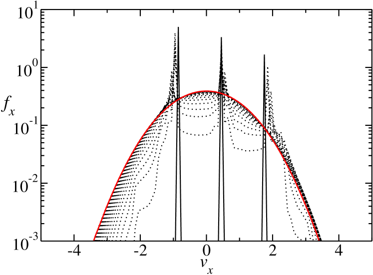
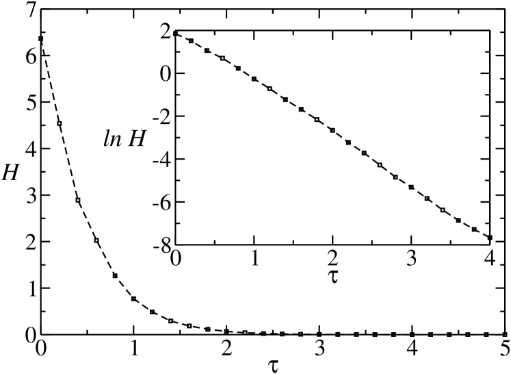
Figure 1: Free cooling. Left) (color online) DSMC results for $f_{x}$ with an initial asymmetric velocity distribution made up of three sharp peaks. The parameters are $\alpha=0.9$ and $N=1000$ and the results have been averaged over $10^{5}$ realizations. The distribution is plotted for different values of the number of collisions per particle $\tau$. The black solid line corresponds to the initial distribution and the bell-shaped red solid line to the distribution at the end of the simulation ($\tau\simeq 14$). Note that the $y$-scale is logarithmic to better probe the low probability region. Right) Corresponding evolution of ${\mathscr{H}}(t)$. The inset shows the same data on a linear-log scale.

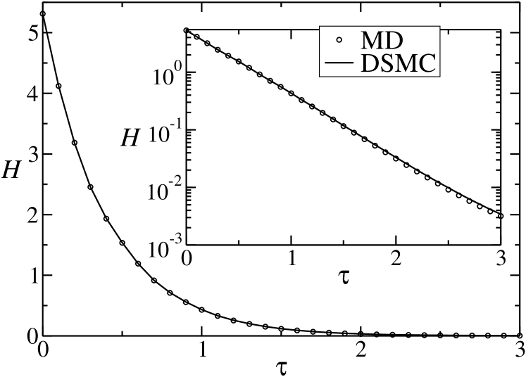
Figure 2: Free cooling. Evolution of ${\mathscr{H}}(t)$ as a function of the number of collisions per particle for MD and DSMC simulations, for an asymmetric initial velocity distribution. Here $\alpha=0.8$, $N=1000$ and the results have been averaged over $5\times 10^{3}$ realizations. The inset shows the same data on a linear-log scale, to emphasize the long time behavior.

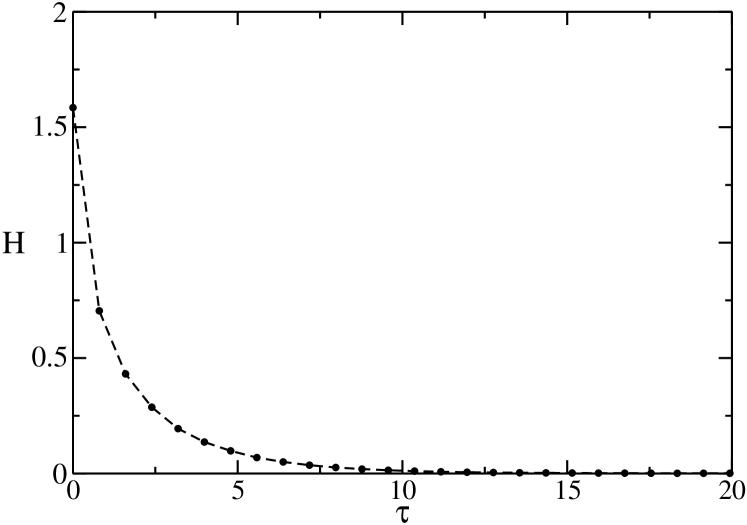
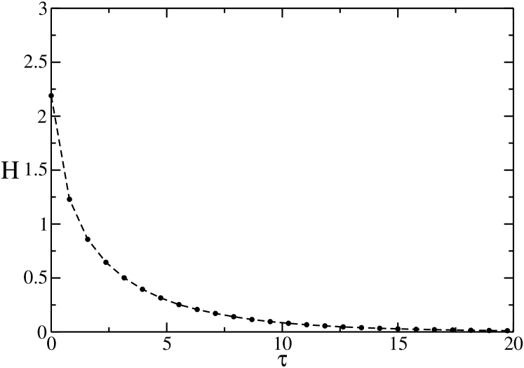
Figure 3: Left) DSMC results of the time evolution of ${\mathscr{H}}(\tau)$ for the the stochastic thermostat for $\alpha=0.9$, starting with a flat distribution. Right) The same but for $\alpha=0.95$.

In Fig. 3, DSMC results are shown for a system heated by the stochastic thermostat. We have considered two values of the inelasticity, $\alpha=0.9$ and $\alpha=0.95$, with an amplitude of the noise, $\xi$, such that the stationary temperature is $8.80T(0)$ for $\alpha=0.9$ and $17.13T(0)$ for $\alpha=0.95$. In the two cases, we have started with the same initial flat distribution, in which all the velocities have the same probability in a square centered in the origin in the velocity space

$$f(\mathbf{v},0)=\left\{\begin{array}[]{ll}\frac{1}{4w^{2}},&\textrm{if $v_{x}\in[-w,w]$ and $v_{y}\in[-w,w]$ }\\ 0,&\textrm{otherwise}\end{array}\right.$$

with $w=\left[\frac{6T(0)}{m}\right]^{1/2}$. The results have been averaged over $10^{5}$ trajectories. Clearly, as in the previous case, the functional $\mathscr{H}$ decays monotonically for all times. Again, as in the Gaussian thermostat case, the same qualitative behavior is obtained for other initial conditions and values of the inelasticity.

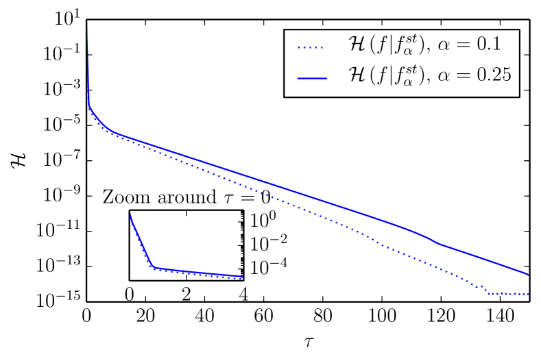
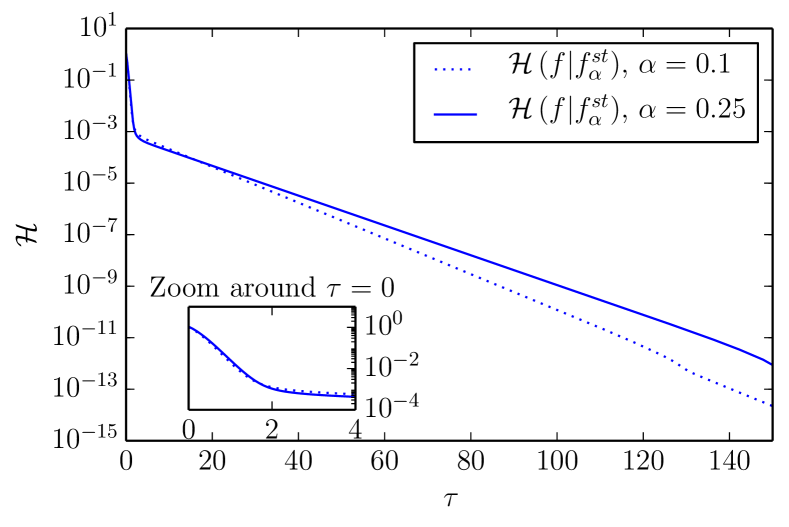
Figure 4: Left) Time evolution of the entropy for the nonlinear Boltzmann equation with stochastic thermostat, solved with the spectral scheme ($M=64$), for $\alpha=0.25$ (solid line) and $\alpha=0.1$ (dotted line), starting with the assymetric, three sharp peaks. Right) Same, for the flat initial distribution.

Finally, we present in Fig. 4 the evolution of $\mathscr{H}$ for small normal restitution coefficients, namely $\alpha=0.1$ (almost sticky particles) and $\alpha=0.25$, in the stochastic thermostat case. The spectral scheme is used for these simulations. We show our results for both the assymetric distribution (45) composed of three peaks (left) and for the flat distribution (right). As in the other simulations, we observe in all these cases a monotone decay of the entropy functional $\mathscr{H}$. Thanks to the accuracy of the spectral scheme, and owing to its deterministic nature, we can observe this decay up to the machine precision. Although it may be due to numerical artifacts (this behavior can be also observed in the elastic case $\alpha=1$), this decay seems to follow two exponential regimes, a very fast one in short time followed by a slower one in larger time. Nevertheless, these decays are always exponential.

All the simulation results point in the same direction: the functional $\mathscr{H}$ defined by Eq. (42) can be a good Lyapunov functional for the free-cooling case (Gaussian thermostat) and for the stochastic thermostat. It is worth emphasizing here that considering the naive functional of the type $\int f\log f$ instead of the Kullback-Leibler distance (42) may lead to non-monotonic behaviour, as shown in mpv13 .

V Conclusions

In this paper, we have presented strong hints that the functional given by Eq. (42) can play the role of a Lyapunov functional in the context of a dissipative granular gas: it decays monotonically in time, tending to zero in the late time non-equilibrium steady state. These results, in agreement with those of Ref mpv13 , have been shown by three different kinds of simulation methods, for a wide class of initial conditions and a wide range of inelasticities, $0<\alpha<1$. Our functional –that takes the form of a relative entropy, or Kullback-Leibler distance– reduces to Boltzmann’s original $\mathscr{H}$ in the case of elastic interactions. Its very form can be directly inspired from information theory, where the Kullback-Leibler distance plays a prominent role CT .

It should be noted that the asymptotic steady state $f_{st}$ enters the definition (42), so that we cannot deduce the form of the non-equilibrium steady or scaling solution from our functional. This is at variance with the reversible dynamics case (elastic collisions, corresponding to $\alpha=1$ above), and is the price for losing the energy conservation law. We emphasize that we have not been able to prove analytically our central result, which requires to work at Boltzmann equation level. The situation is simpler at $N$-body level, where a counterpart of the $H$-theorem can be shown. We nevertheless believe our result is conceptually important; monotonicity of ${\mathscr{H}}(t)$ with time is a strong statement, the derivation of which has been the focus of some effort in the past.

In the particular free cooling case, we have shown that the $N$-particle velocity distribution function reaches an auto-similar regime in which all its time dependence is encoded in the instantaneous temperature [a similar scaling has already been used in the context of the Liouville equation (with spatial dependence) BDS97 ]. A comparable analysis can be put forward for mixtures, binary or polydisperse, where the existence of a scaling solution implies the coincidence of the different cooling rates.

Appendix A Evolution equation for the temperature in the free-cooling case

Assuming the scaling form of the main text, Eq. (9), the evolution equation for the temperature can be straightforwardly obtained by taking the second velocity moment in Eq. (3). The result is

$$\frac{dT(t)}{dt}=-\bar{B}T(t)^{\frac{\gamma}{2}+1},$$ (46)

where we have introduced the time-independent coefficient

$$\bar{B}=\frac{KA\langle c_{12}^{\gamma+2}\rangle}{4d}\left(\frac{2}{m}\right)^{\gamma/2}(1-\alpha^{2}),$$ (47)

with

$$A=\int d\boldsymbol{\hat{\sigma}}\hat{\sigma}_{x}^{\gamma+2},\quad\langle c_{12}^{\gamma+2}\rangle=\int d\mathbf{c}_{1}\int d\mathbf{c}_{2}c_{12}^{\gamma+2}\varphi_{2}(\mathbf{c}_{1},\mathbf{c}_{2}).$$ (48)

The function $\varphi_{2}$ is just the integrated scaled distribution, $\varphi_{2}(\mathbf{c}_{1},\mathbf{c}_{2})=\int d\mathbf{c}_{3}\dots\int d\mathbf{c}_{N}\varphi_{N}(\mathbf{C})$. Eq. (46) can be readily integrated, leading to the

$$T(t)=\left[\frac{1}{T(0)^{\gamma/2}}+\frac{\gamma\bar{B}}{2}t\right]^{-\frac{2}{\gamma}},\qquad\textrm{for $\gamma>0$},$$ (49)

and

$$T(t)=T(0)e^{-\bar{B}t}\qquad\textrm{for $\gamma=0$}.$$ (50)

Then, for $\gamma>0$ the temperature ‘forgets’ the initial condition in the long time limit and behaves as

$$T(t)\approx\left(\frac{\gamma\bar{B}}{2}t\right)^{-2/\gamma},\qquad\textrm{for $t\to\infty$}.$$ (51)

We point now that the scaling given by Eq. (9) is compatible with Kac’s equation, Eq. (3). By substituting Eq. (9) into Eq. (3), the following equation for $\varphi_{N}$ is obtained

$$\frac{1}{Kv_{H}^{\gamma+1}}\frac{dv_{H}(t)}{dt}\frac{\partial}{\partial\mathbf{C}}\cdot\mathbf{C}\varphi_{N}(\mathbf{C})+\frac{1}{N}\sum_{i<j}L(\mathbf{c}_{i},\mathbf{c}_{j})\varphi_{N}(\mathbf{C})=0,$$ (52)

where $\mathbf{C}=\mathbf{V}/v_{H}(t)$. As a consequence of Eq. (46), the term $\frac{1}{Kv_{H}^{\gamma+1}}\frac{dv_{H}(t)}{dt}$ is time-independent, and thus, Eq. (52) is consistent.

Appendix B Evaluation of $\frac{d\mathscr{H}_{N}(s)}{ds}$

Before evaluating $\frac{d\mathscr{H}_{N}(s)}{ds}$, let us note that Eq. (14) can be written as a Master equation

$$\frac{\partial}{\partial s}\phi_{N}(\mathbf{C},s)=\int d\mathbf{U}\mathscr{W}(\mathbf{C}|\mathbf{U})\phi_{N}(\mathbf{U},s)-\int d\mathbf{U}\mathscr{W}(\mathbf{U}|\mathbf{C})\phi_{N}(\mathbf{C},s),$$ (53)

with the transition probabilities per unit time, $\mathscr{W}(\mathbf{U}|\mathbf{C})$, given by

$$\mathscr{W}(\mathbf{U}|\mathbf{C})=\mathscr{W}_{C}(\mathbf{U}|\mathbf{C})+\mathscr{W}_{T}(\mathbf{U}|\mathbf{C}),$$ (54)

where

$$\mathscr{W}_{C}(\mathbf{U}|\mathbf{C})=\frac{1}{N}\sum_{i<j}\int d\boldsymbol{\hat{\sigma}}(\mathbf{c}_{ij}\cdot\boldsymbol{\hat{\sigma}})^{\gamma}\delta(\mathbf{u}_{i}-\mathbf{c}_{i}^{\prime})\delta(\mathbf{u}_{j}-\mathbf{c}_{j}^{\prime})\Pi_{k\neq i,j}\delta(\mathbf{u}_{k}-\mathbf{c}_{k}),$$ (55)

is the contribution due to collision and

$$\mathscr{W}_{T}(\mathbf{U}|\mathbf{C})=-\frac{B}{2}\mathbf{C}\cdot\frac{\partial}{\partial\mathbf{U}}\delta(\mathbf{U}-\mathbf{C}),$$ (56)

the contribution of the thermostat.

Following the same steps as van Kampen kampen , it is obtained that

$$\frac{d\mathscr{H}_{N}(s)}{ds}=\int d\mathbf{C}\int d\mathbf{U}\mathscr{W}(\mathbf{C}|\mathbf{U})\phi_{N}^{st}(\mathbf{U})\left\{[x(\mathbf{U},s)-x(\mathbf{C},s)]h^{\prime}[x(\mathbf{C},s)]\right.$$

$$\left.+h[x(\mathbf{C},s)]-h[x(\mathbf{U},s)]\right\},$$ (57)

where

$$x(\mathbf{C},s)=\frac{\phi_{N}(\mathbf{C},s)}{\phi_{N}^{st}(\mathbf{C})}.$$ (58)

It can be seen that the contribution coming from the thermostat vanishes. Indeed,

$$\int d\mathbf{C}\int d\mathbf{U}\mathscr{W}_{T}(\mathbf{C}|\mathbf{U})\phi_{N}^{st}(\mathbf{U})\left\{[x(\mathbf{U},s)-x(\mathbf{C},s)]h^{\prime}[x(\mathbf{C},s)]+h[x(\mathbf{C},s)]-h[x(\mathbf{U},s)]\right\}$$

$$=\frac{B}{2}\int d\mathbf{C}\int d\mathbf{U}\delta(\mathbf{U}-\mathbf{C})\phi_{N}^{st}(\mathbf{U})\mathbf{U}\cdot\frac{\partial}{\partial\mathbf{C}}\left\{[x(\mathbf{U},s)-x(\mathbf{C},s)]h^{\prime}[x(\mathbf{C},s)]\right.$$

$$\left.+h[x(\mathbf{C},s)]-h[x(\mathbf{U},s)]\right\}=0.$$ (59)

The collisional counterpart can be written as

$$\int d\mathbf{C}\int d\mathbf{U}\mathscr{W}_{C}(\mathbf{C}|\mathbf{U})\phi_{N}^{st}(\mathbf{U})\left\{[x(\mathbf{U},s)-x(\mathbf{C},s)]h^{\prime}[x(\mathbf{C},s)]+h[x(\mathbf{C},s)]-h[x(\mathbf{U},s)]\right\}$$

$$=\frac{N-1}{2}\int d\mathbf{C}\int d\boldsymbol{\hat{\sigma}}(\mathbf{c}_{12}\cdot\boldsymbol{\hat{\sigma}})^{\gamma}\phi_{N}^{st}(\mathbf{C})\left\{h[x(\mathbf{C}^{\prime},s)]-h[x(\mathbf{C},s)]+h^{\prime}[x(\mathbf{C}^{\prime},s)][x(\mathbf{C},s)-x(\mathbf{C}^{\prime},s)]\right\},$$

where we have introduced the notation $\mathbf{C}^{\prime}=\{\mathbf{c}_{1}^{\prime},\mathbf{c}_{2}^{\prime},\mathbf{c}_{3},\dots,\mathbf{c}_{N}\}$ and we have used that, due to the invariance of $\phi_{N}(\mathbf{C},s)$ under the change of labels $\mathbf{c}_{i}\leftrightarrow\mathbf{c}_{j}$ for any $i$ and $j$, the $N(N-1)/2$ collisional terms are equal. By substituting Eqs (B) and (B) into (B), the expression of the main text is obtained.

Appendix C Consistency of Kac’s equation in the stochastic thermostat case

In this appendix, it is shown that the conservation of the total momentum assumed by the thermostat is essential to ensure that Eq. (22) be compatible with the existence of a stationary state. We assume that a stationary solution of Eq. (22) exists, $\rho_{N}^{st}(\mathbf{V})$. It then fulfills

$$\frac{K}{N}\sum_{i<j}L(\mathbf{v}_{i},\mathbf{v}_{j})\rho_{N}^{st}(\mathbf{V})+\xi_{0}^{2}T(\mathbf{V})\rho_{N}^{st}(\mathbf{V})=0.$$ (61)

Let us multiply the equation by $v_{1}^{2}$ and integrate. The collisional contribution is

$$\frac{K}{N}\sum_{i<j}\int\,{\rm d}\mathbf{v}v_{1}^{2}L(\mathbf{v}_{i},\mathbf{v}_{j})\rho_{N}^{st}(\mathbf{V})$$

$$=\frac{K(N-1)}{2N}\int\,{\rm d}\mathbf{v}\rho_{N}^{st}(\mathbf{V})\int d\boldsymbol{\hat{\sigma}}(\boldsymbol{\hat{\sigma}}\cdot\mathbf{v}_{12})^{\gamma}(b_{\boldsymbol{\hat{\sigma}}}-1)(v_{1}^{2}+v_{2}^{2})$$

$$=-\frac{K(N-1)}{4N}(1-\alpha^{2})\int\,{\rm d}\mathbf{v}\rho_{N}^{st}(\mathbf{V})\int d\boldsymbol{\hat{\sigma}}(\boldsymbol{\hat{\sigma}}\cdot\mathbf{v}_{12})^{\gamma+2},$$ (62)

where use has been made of

$$(b_{\boldsymbol{\hat{\sigma}}}-1)(v_{1}^{2}+v_{2}^{2})=-\frac{1-\alpha^{2}}{2}(\boldsymbol{\hat{\sigma}}\cdot\mathbf{v}_{12})^{2}.$$ (63)

The thermostat contribution is

$$\xi_{0}^{2}\int\,{\rm d}\mathbf{v}v_{1}^{2}T(\mathbf{V})\rho_{N}^{st}(\mathbf{V})=\frac{\xi_{0}^{2}}{2}\int\,{\rm d}\mathbf{v}\rho_{N}^{st}(\mathbf{V})\frac{\partial^{2}}{\partial v_{1}^{2}}v_{1}^{2}=d\xi_{0}^{2},$$ (64)

where the cross-terms do not contribute. The obtained equation is

$$\frac{K(N-1)}{4N}(1-\alpha^{2})\int\,{\rm d}\mathbf{v}\rho_{N}^{st}(\mathbf{V})\int d\boldsymbol{\hat{\sigma}}(\boldsymbol{\hat{\sigma}}\cdot\mathbf{v}_{12})^{\gamma+2}=d\xi_{0}^{2}.$$ (65)

Keeping in mind the above ‘steady-state constraint’, let us now multiply Eq. (61) by $\mathbf{v}_{1}\cdot\mathbf{v}_{2}$ and integrate. The collisional contribution is

$$\frac{K}{N}\sum_{i<j}\int\,{\rm d}\mathbf{v}\mathbf{v}_{1}\cdot\mathbf{v}_{2}L(\mathbf{v}_{i},\mathbf{v}_{j})\rho_{N}^{st}(\mathbf{V})$$

$$=\frac{K}{N}\int\,{\rm d}\mathbf{v}\rho_{N}^{st}(\mathbf{V})\int d\boldsymbol{\hat{\sigma}}(\boldsymbol{\hat{\sigma}}\cdot\mathbf{v}_{12})^{\gamma}(b_{\boldsymbol{\hat{\sigma}}}-1)\mathbf{v}_{1}\cdot\mathbf{v}_{2}$$

$$=\frac{K}{4N}(1-\alpha^{2})\int\,{\rm d}\mathbf{v}\rho_{N}^{st}(\mathbf{V})\int d\boldsymbol{\hat{\sigma}}(\boldsymbol{\hat{\sigma}}\cdot\mathbf{v}_{12})^{\gamma+2},$$ (66)

where it has been used that

$$(b_{\boldsymbol{\hat{\sigma}}}-1)\mathbf{v}_{1}\cdot\mathbf{v}_{2}=\frac{1-\alpha^{2}}{4}(\boldsymbol{\hat{\sigma}}\cdot\mathbf{v}_{12})^{2}.$$ (67)

From the conservation of total momentum in a collision, we further have $(b_{\boldsymbol{\hat{\sigma}}}-1)(\mathbf{v}_{1}+\mathbf{v}_{2})^{2}=0$, so that

$$(b_{\boldsymbol{\hat{\sigma}}}-1)\mathbf{v}_{1}\cdot\mathbf{v}_{2}=-\frac{1}{2}(b_{\boldsymbol{\hat{\sigma}}}-1)(v_{1}^{2}+v_{2}^{2}),$$ (68)

from Eqs. (63) and (67). The thermostat contribution is

$$\xi_{0}^{2}\int\,{\rm d}\mathbf{v}\mathbf{v}_{1}\cdot\mathbf{v}_{2}T(\mathbf{V})\rho_{N}^{st}(\mathbf{V})$$

$$=-\frac{\xi_{0}^{2}}{N-1}\int\,{\rm d}\mathbf{v}\rho_{N}^{st}(\mathbf{V})\frac{\partial}{\partial\mathbf{v}_{1}}\frac{\partial}{\partial\mathbf{v}_{2}}\mathbf{v}_{1}\cdot\mathbf{v}_{2}=-\frac{d\xi_{0}^{2}}{N-1},$$ (69)

where only the cross-terms contribute. The obtained equation is equivalent to Eq. (65) but, as indicated above, only because of the presence of the cross terms [second term on the right hand side of Eq. (19)]. In other words, it is essential that the thermostat conserve total momentum, otherwise, the center-of-mass of the system undergoes a Brownian motion in velocity space, incompatible with the existence of a steady state PSD13 .

References

- (1) L. Boltzmann, Wiener Berichte 66, 275 (1872), also paper 23 in Wissenschaftliche Abhandlungen, Vol. I, F. Hasenöhrl (ed.), Leipzig: Barth (1909); reissued New York: Chelsea (1969).
- (2) see e.g. C. Villani, A review of mathematical topics in collisional kinetic theory, in Handbook of Mathematical Fluid Dynamics, S. Friedlander and D. Serre, Eds, Elsevier Science (2002).
- (3) Transport Phenomena and Kinetic Theory, edited by C. Cercignani and E. Gabetta, Birkhäuser Boston, (2007).
- (4) N. Bellomo, Modelling Complex Living Systems: A Kinetic Theory and Stochastic Game Approach (Modelling and Simulation in Science, Engineering and Technology), Birkhäuser Boston, (2007).
- (5) L. Boltzmann, Lectures on gas theory. Reprint of the 1896-1898 Edition. Reprinted by Dover Publications, 1995.
- (6) C. Cercignani, The Boltzmann equation and its applications, Springer-Verlag (1988).
- (7) It should be noted here that Boltzmann’s functional clearly is a forerunner of Shannon’s information measure, introduced more than 70 years later Shannon . This measure is of paramount importance in data and signal analysis or transmission. It should also be stressed that the -theorem today still is a remarkable source of inspiration to attack many mathematical problems (see e.g. Ref Villani ), socio-physics questions (see e.g. Ref Apenko ) or to find new classes of time dependent exact solutions to the Boltzmann equation under confinement dgo .
- (8) The -theorem essentially holds for dilute hard core systems (with negligible internal energy compared to the kinetic energy), see e.g. E.T. Jaynes, Phys. Rev. A 4, 747 (1971) for a discussion of the “violations” occurring in real gases. See also P.L. Garrido, S. Goldstein and J.L. Lebowitz, Phys. Rev. Lett. 92, 050602 (2004) for a more recent and precize account.
- (9) S.G. Brush, The Kind of Motion We Call Heat, Amsterdam, North Holland (1976).
- (10) C. Cercignani, Ludwig Boltzmann, the man who trusted atoms, Oxford University Press (1998).
- (11) J.L. Lebowitz, Rev. Mod. Phys. 71, S346 (1999).
- (12) I. Goldhirsch, Annu. Ref. Fluid Mech. 35, 267 (2003).
- (13) N. Brilliantov and T. Poschel, Kinetic Theory of Granular Gases, Oxford University Press (2004).
- (14) C. Villani, J. Stat. Phys. 124, 781 (2006).
- (15) I. Bena, F. Coppex, M. Droz, P. Visco, E. Trizac and F. van Wijland, Physica A 370, 179 (2006).
- (16) A. Barrat, E. Trizac and M.H. Ernst, J. Phys. Condens. Matter 17, S2429 (2005).
- (17) A. Goldshtein and M. Shapiro, J. Fluid Mech. 282, 75 (1995).
- (18) S. Mischler, C. Mouhot and M. Rodriguez Ricard, J. Stat. Phys. 124, 2–4 (2006); S. Mischler and C. Mouhot, J. Stat. Phys. 124, 2–4 (2006); S. Mischler and C. Mouhot, Comm. Math. Phys. 288, 2 (2009).
- (19) A.V. Bobylev, C. Cercignani, J. Statist. Phys. 110, 1–2 (2003), J. Statist. Phys. 111 1–2 (2003).
- (20) S. Mischler and C. Mouhot, Discrete Contin. Dyn. Syst. 24, 1 (2009).
- (21) J.J. Brey, J.W. Dufty and A. Santos, J. Stat. Phys. 87, 1051 (1997).
- (22) U.M.B. Marconi, A. Puglisi, and A. Vulpiani, J. Stat. Mech. (2013) P08003.
- (23) M.H. Ernst, E. Trizac and A. Barrat, J. Stat. Phys. 124, 549 (2006).
- (24) M. Kac, Foundations of Kinetic Theory, Proc. 3rd Berkeley Symp. Math. Stat. Prob., Univ. of California Press, vol. 3, 171 (1956).
- (25) J. F. Lutsko, Phys. Rev. E 63, 061211 (2001).
- (26) J.J. Brey, M.J. Ruiz-Montero, and F. Moreno, Phys. Rev. E 69, 051303 (2004).
- (27) N. G. van Kampen, Stochastic Processes in Physics and Chemistry (North-Holland, 2007).
- (28) J.M. Montanero and A. Santos, Granular Matter 2, 53 (2000).
- (29) T.P.C. van Noije, and M.H. Ernst, Granular Matter 1, 57 (1998).
- (30) T.P.C. van Noije, M.H. Ernst, E. Trizac, and I. Pagonabarraga, Phys. Rev. E 59, 4326 (1999).
- (31) See also A. Puglisi, V. Loreto, U.M.B. Marconi, A. Petri and A. Vulpiani, Phys. Rev. Lett. 81 3848 (1998) for a slight variant of the model.
- (32) M. I. García de Soria, P. Maynar, and E. Trizac, Molec. Phys. 107, 383 (2009).
- (33) V. V. Prasad, S. Sabhapandit1 and A. Dhar, EPL 104, 54003 (2013).
- (34) E. Carlen, M.C. Carvalho, J. Le Roux, M. Loss, C. Villani, Kinet. Relat. Models 3, 1, (2010).
- (35) S. Mischler and C. Mouhot, Invent. Math. 193, 1 (2013).
- (36) M. Hauray and S. Mischler, J. Funct. Anal. 266, 10 (2014).
- (37) K. Carrapatoso, Ann. Inst. H. Poincaré Probab. Statist. 51, 993 (2015).
- (38) S. Mischler, C. Mouhot and B. Wennberg, Probab. Theory Relat. Fields 161, 1-2 (2015).
- (39) T.M. Cover and J.M. Thomas, Elements of Information Theory, 2nd Edition, New York: Wiley-Interscience (2006).
- (40) L. Pareschi and B. Perthame, Transport Theory Statist. Phys. 25, 369 (1996).
- (41) F. Filbet and L. Pareschi, and G. Toscani, J. Comp. Phys. 202, 216 (2005).
- (42) P. Maynar and E. Trizac, Phys. Rev. Lett. 106, 160603 (2011).
- (43) G. A. Bird, Molecular Gas Dynamics and the Direct Simulation of Gas Flows, Claredon, Oxford (1994).
- (44) M. P. Allen and D. J. Tildesley, Computer Simulation of Liquids, Oxford Science Publications, Bristol, (1987).
- (45) Molecular Dynamics simulations are more demanding in the driven case, particularly so if small densities are considered.
- (46) S. McNamara, Phys. Fluids A 5, 3056 (1993); I. Goldhirsch, M.-L. Tan and G. Zanetti, J. Sci. Comput. 8, 1 (1993); J.J. Brey, M.J. Ruiz-Montero, and D. Cubero, Phys. Rev. E 54, 3664 (1996); P. Deltour and J.-L. Barrat, J. Phys. 17,137 (1997).
- (47) C.E. Shannon, Bell Syst. Tech. Journal 27, 379 (1948); ibid. 27, 623 (1948).
- (48) C. Villani, -Theorem and beyond: Boltzmann’s entropy in today’s mathematics, in Boltzmann’s legacy, ESI Lect. Math. Phys., G. Gallavotti, W.L. Reiter and J. Yngvason eds, Eur. Math. Soc., Zürich, pp.129-143 (2008).
- (49) S.M. Apenko, Phys. Rev. E 87, 024101 (2013).
- (50) D. Guéry-Odelin, J.G. Muga, M.J. Ruiz Montero and E. Trizac, Phys. Rev. Lett. 112, 180602 (2014).