On Practical SMT-Based Type Error Localization

Abstract

Compilers for statically typed functional programming languages are notorious for generating confusing type error messages. When the compiler detects a type error, it typically reports the program location where the type checking failed as the source of the error. Since other error sources are not even considered, the actual root cause is often missed. A more adequate approach is to consider all possible error sources and report the most useful one subject to some usefulness criterion. In our previous work, we showed that this approach can be formulated as an optimization problem related to satisfiability modulo theories (SMT). This formulation cleanly separates the heuristic nature of usefulness criteria from the underlying search problem. Unfortunately, algorithms that search for an optimal error source cannot directly use principal types which are crucial for dealing with the exponential-time complexity of the decision problem of polymorphic type checking. In this paper, we present a new algorithm that efficiently finds an optimal error source in a given ill-typed program. Our algorithm uses an improved SMT encoding to cope with the high complexity of polymorphic typing by iteratively expanding the typing constraints from which principal types are derived. The algorithm preserves the clean separation between the heuristics and the actual search. We have implemented our algorithm for OCaml. In our experimental evaluation, we found that the algorithm reduces the running times for optimal type error localization from minutes to seconds and scales better than previous localization algorithms.

1 Introduction

Hindley-Milner type systems support automatic type inference, which is one of the features that make languages such as Haskell, OCaml, and SML so attractive. While the type inference problem for these languages is well understood [10, 19, 16, 30, 1, 23], the problem of diagnosing type errors still lacks satisfactory solutions [32, 12, 31, 14, 9, 8, 21, 17, 24].

When type inference fails, a compiler usually reports the location where the first type mismatch occurred as the source of the error. However, often the actual location that is to blame for the error and needs to be fixed is somewhere else entirely. Consequently, the quality of type error messages suffers, which increases the debugging time for the programmer. A more adequate approach is to consider all possible error sources and then choose the one that is most likely to blame for the error. Here, an error source is a set of program locations that, once corrected, yield a well-typed program.

The challenge for this approach is that it involves two subproblems that are difficult to untangle: (1) searching for type error sources, and (2) ranking error sources according to some usefulness criterion (e.g., the number of required modifications to fix the program). Existing solutions to type error localization make specific heuristic decisions for solving these subproblems. As a consequence, the resulting algorithms often do not provide formal guarantees or use specific usefulness criteria that are difficult to justify or adapt. In our recent work [24], we have proposed a novel approach that formalizes type error localization as an optimization problem. The advantage of this approach is that it creates a clean separation between (1) the algorithmic problem of finding error sources of minimum cost, and (2) the problem of finding good usefulness criteria that define the cost function. This separation of concerns allows us to study these two problems independently. In this paper, we develop an efficient solution for problem (1).

Challenge.  Type inference is often formalized in terms of constraint satisfaction [30, 1, 23]. In this formalization, each expression in the program is associated with a type variable. A typing constraint of a program encodes the relationship between the type of each expression and the types of its subexpressions by constraining the type variables appropriately. The program is then well-typed iff there exists an assignment of types to the type variables that satisfies the constraint. In our previous paper, we used this formalization to reduce the problem of finding minimum error sources to a known optimization problem in satisfiability modulo theories (SMT), the partial weighted MaxSMT problem. This reduction enables us to use existing MaxSMT solvers for type error localization.

The reduction to constraint satisfaction also has its problems. The number of typing constraints can grow exponentially in the size of the program. This is because the constraints associated with polymorphic functions are duplicated each time these functions are used. This explosion in the constraint size does not seem to be avoidable because the type inference problem is known to be EXPTIME-complete [19, 16]. However, in practice, compilers successfully avoid the explosion by computing the principal type [10] of each polymorphic function and then instantiating a fresh copy of this type for each usage. The resulting constraints are much smaller in practice. Since the smaller constraints are equisatisfiable with the original constraints, the resulting algorithm is a decision procedure for the type checking problem [10]. Unfortunately, this technique cannot be applied immediately to the optimization problem of type error localization. If the minimum cost error source is located inside of a polymorphic function, then abstracting the constraints of that function by its principle type will hide this error source. Thus, this approach can yield incorrect results. This dilemma is inherent to all type error localization techniques and the main reason why existing algorithms that are guaranteed to produce optimal solutions do not yet scale to real-world programs.

Solution.  Our new algorithm makes the optimistic assumption that the relevant type error sources only involve few polymorphic functions, even for large programs. Based on this assumption, we propose an improved reduction to the MaxSMT problem that abstracts polymorphic functions by principal types. The abstraction is done in such a way that all potential error sources involving the definition of an abstracted function are represented by a single error source whose cost is smaller or equal to the cost of all these potential error sources. The algorithm then iteratively computes minimum error sources for abstracted constraints. If an error source involves a usage of a polymorphic function, the corresponding instantiations of the principal type of that function are expanded to the actual typing constraints. Usages of polymorphic functions that are exposed by the new constraints are expanded if they are relevant for the minimum error source in the next iteration. The algorithm eventually terminates when the computed minimum error source no longer involves any usages of abstracted polymorphic functions. Such error sources are guaranteed to have minimum cost for the fully expanded constraints, even if the final constraint is not yet fully expanded.

We have implemented our algorithm targeting OCaml [22] and evaluated it on benchmarks for type error localization [17] as well as code taken from a larger OCaml application. We used EasyOCaml [13] for generating typing constraints and the MaxSMT solver $\nu$Z [7, 6, 11] for computing minimum error sources. We found that our implementation efficiently computes the minimum error source in our experiments for a typical usefulness criterion taken from [24]. In particular, our algorithm is able to compute minimum error sources for realistic programs in seconds, compared to several minutes for the naive algorithm and other approaches. Also, on our benchmarks, the new algorithm avoids the exponential explosion in the size of the generated constraints that we observe in the naive algorithm.

Related Work.  The formulation of type error localization as an optimization problem follows our previous work [24]. There, we presented the naive implementation of the search algorithm. Other work on type error localization is not directly comparable to ours. Most closely related is the work by Zhang and Myers [33, 34] where type error localization is cast as a graph analysis problem. Their approach, however, does not address the issue of constraint explosion, which here manifests as an explosion in the size of the generated graphs. In fact, our algorithm is faster than their implementation on the same benchmarks: while their tool runs over a minute for some programs, our algorithm always finishes in a just of a couple of seconds. Consequently, for larger problem instances with a couple of thousands of lines of code their implementation runs out of memory. Our algorithm, on the other hand, finishes in less than 50 seconds. The majority of the remaining work on type error localization is concerned with different definitions and notions of usefulness criteria [32, 12, 31, 14, 9, 8, 21]. In our previous work, we gave experimental evidence that our approach yields better error sources than the OCaml compiler even for a relatively simple cost function. The work in this paper is orthogonal because it focuses on practical algorithms for computing a minimum error source subject to an arbitrary cost function.

Contributions.  Our contributions can be summarized as follows:

• We present a new algorithm that uses SMT techniques to efficiently find the minimum error source in a given ill-typed program. The algorithm works for an arbitrary cost function which encodes the usefulness criterion for ranking error sources.

• We have implemented the algorithm and showed that it scales to programs of realistic size.

• To our knowledge, this is the first algorithm for type error localization that gives formal optimality guarantees and has the potential to be usable in practice.

2 Overview

In this section we provide an overview of our approach through an illustrative example. We start by describing type error localization as an optimization problem and then exemplify the workings of our algorithm that efficiently solves the problem.

2.1 Example

Our running OCaml example is as follows:

⬇

1let first (a, b, _) = a

2let second (a, b, _) = b

3let f x =

4 let first_x = first x in

5 let second_x = int_of_string (second x) in@\label{code:ok-call}first_x + second_x f ("1", "2", f ("3", "4", 5))\label{code:error}

This program is not well-typed. While polymorphic functions first, second, and f do not have any type errors, the calls to f on line LABEL:code:error are ill-typed. The inner call to f is passed a triple having the string "3" as its first member, whereas an integer is expected. The standard OCaml compiler [22] reports this type error to the programmer blaming expression "1" on line LABEL:code:error as the source of the error (OCaml version $4.01.0$). However, perhaps the programmer made a mistake by calling function first on line 4 or maybe she incorrectly defined first on line 1. Maybe the programmer should have wrapped this call with a call to int_of_string just as she has done on line LABEL:code:ok-call. The OCaml compiler disregards such error sources.

2.2 Finding Minimum Error Sources

In our previous work [24], we formulated type error localization as an optimization problem of finding an error source that is considered most useful for the programmer. The criterion for usefulness is provided by the compiler. We define an error source to be a set of program expressions that, once fixed, make the program well-typed. A usefulness criterion is a function from program expressions to positive weights. A minimum error source is an error source with minimum cumulative weight. It corresponds to the most useful error source. To make this more clear, consider a usefulness criterion where each expression is assigned a weight equal to the size of the expression, represented as an abstract syntax tree (AST). In the example, expression first on line 4 is a singleton error source of weight $1$ as replacing it by a function of a type that is an instance of the polymorphic type

$$\forall\alpha.\mathsf{fun}(\mathsf{string}*\mathsf{string}*\alpha,\mathsf{int}),$$

makes the program well-typed, say int_of_string$\;\circ\;$first. Similarly, replacing the expression a on line 1 with (int_of_string a) also resolves the type error. Loosely speaking, the error sources that are minimum subject to the AST size criterion require the fewest corrections to fix the error. The two error sources described above are minimum error sources since their cumulative weight is $1$, which is minimum for this program and criterion. In contrast, we could abstract the entire application first x on the same line to get a well typed program. Thus first x is also an error source, but it is not minimum as its weight is $3$ according to its AST size (first, x, and function application). Note that "1" on line LABEL:code:error on its own is not an error source according to our definition. If one abstracts "1", this does not yield a well typed program since the expression "3" on line LABEL:code:error would still lead to a failure. Abstracting both $\{\texttt{"1"},\texttt{"3"}\}$ is an error source with cumulative weight 2. Observe that there is a clean separation between searching for a minimum error source and the definition of the usefulness criterion. This allows easy prototyping of various criteria without modifying the compiler infrastructure. A more detailed discussion of potential usefulness criteria can be found in [24].

2.3 Abstraction by Principal Types

A potential obstacle to adopting this approach is that compilers now need to solve an optimization problem instead of a decision problem. This is particularly problematic since type checking for polymorphic type systems is EXPTIME complete [19, 16]. This high complexity manifests in an exponential number of generated typing constraints. For instance, consider the typing constraints for the function second:

$$\alpha_{\mathit{second}} =\mathsf{fun}(\alpha_{i},\alpha_{o})$$ [Def. of second] (1)

$$\alpha_{i} =\mathsf{triple}(\alpha_{a},\alpha_{b},\alpha_{\_})$$ (a, b, _) (2)

$$\alpha_{o} =\alpha_{b}$$ b (3)

The above constraints state that the type of second, represented by the type variable $\alpha_{second}$, is a function type (1) that accepts some triple (2) and returns a value whose type is equal to the type of the second component of that triple (3). When a polymorphic function, such as second, is called in the program, the associated set of typing constraints needs to be instantiated and the new copy has to be added to the whole set of typing constraints. Instantiation of typing constraints involves copying the constraints and replacing free type variables in the copy with fresh type variables. In our example, each call to second in f is accounted for by a fresh instance of $\alpha_{second}$ and the whole set of associated typing constraints is copied and instantiated by replacing the type variable $\alpha_{second}$ with a fresh type variable. If the constraints of polymorphic function were not freshly instantiated for each usage of the function, the same type variable would be constrained by the context of each usage, potentially resulting in a spurious type error.

Instantiation of typing constraints as described above leads to an explosion in the total number of generated constraints. For instance, the typing constraints for each call to f are instantiated twice. Each of these copies in turn includes a fresh copy of the constraints associated with each call to second and first in f. Hence, the number of typing constraints can grow exponentially, to the point where the whole approach becomes impractical. To alleviate this problem, compilers first solve the typing constraints for each polymorphic function to get their principal types. Intuitively, the principal type is the most general type of an expression [10]. Then, each time the function is used only its principal type is instantiated, instead of the whole set of associated typing constraints.

In the example, when typing the line LABEL:code:error, the typing environment contains principal types for first, second, and f (given as comments below).

⬇

1; first : $\forall\alpha_{a},\alpha_{b},\alpha_{c}.\;\mathsf{fun}(\alpha_{a}*\alpha_{b}*\alpha_{c},\alpha_{a})$

2; second : $\forall\alpha_{a},\alpha_{b},\alpha_{c}.\;\mathsf{fun}(\alpha_{a}*\alpha_{b}*\alpha_{c},\alpha_{b})$

3; f : $\forall\alpha_{a}.\;\mathsf{fun}(\mathsf{int}*\mathsf{string}*\alpha_{a},\mathsf{int})$

4f ("1", "2", f ("3", "4", 5))

The bodies of the three bound variables and the typing constraints within the bodies are effectively abstracted at this point. Type inference instantiates the principal type of f,

$$\texttt{f}:\forall\alpha.\mathsf{fun}(\mathsf{int}*\mathsf{string}*\alpha,\mathsf{int}),$$

but this will fail to unify with the argument to f which has type string * string * int.

The principal type technique for avoiding the constraint explosion works very well in practice for the decision problem of type checking. However, we will need to adapt it in order to work with the optimization problem of searching for a minimum error source. When the search algorithm checks whether a set of expressions is an error source, it checks satisfiability of the typing constraints that have been generated for the whole program, where the constraints for the expressions in the potential error source have been removed. If we directly use the principal type as an abstraction of the function body, we potentially miss some error sources that involve expressions in the abstracted function body. To illustrate this point, consider the principal type abstraction of our example program above. The application of the expression first at line 4 has in effect been abstracted from the program and cannot be reported as an error source, although it is in fact minimum. In general, fixing an error source in a function definition can change the principal type of that function. The search algorithm must take such changes into account in order to identify the minimum error sources correctly. In our running example, a generic fix to the call to function first at line 4 results in the principal type of f being:

$$\forall\alpha_{a},\alpha_{b}.\mathsf{fun}(\alpha_{a}*\mathsf{string}*\alpha_{b},\mathsf{int}).$$

Additionally, principal types may not exist for some expressions in an ill-typed program. The algorithm needs to handle such cases gracefully.

2.4 Approach

Our solution to this problem is an algorithm that finds a minimum error source by expanding the principal types of polymorphic functions iteratively. We first compute principal types for each let-bound variable whenever possible. We begin our search assuming that none of the usages of the variables whose principal types could be computed are involved in a minimum error source. Each principal type is assigned the minimum weight of all constraints in the associated let definition, conservatively approximating the potential minimum error sources that involve these constraints.

$$\begin{array}[]{lr}P_{\texttt{first}}&1\\ P_{\texttt{second}}&1\\ P_{\texttt{f}}&1\\ \alpha_{f1}=\mathsf{fun}(\alpha_{i1},\alpha_{o1})&11\\ P_{\texttt{f}}\Rightarrow\alpha_{f1}=\mathsf{fun}(\mathsf{int}*\mathsf{string}*\alpha^{\prime},\mathsf{int})&1\\ \alpha_{i1}=\alpha_{\texttt{"}1\texttt{"}}*\alpha_{\texttt{"}2\texttt{"}}*\alpha_{app}&9\\ \alpha_{\texttt{"}1\texttt{"}}=\mathsf{string}&1\\ \alpha_{\texttt{"}2\texttt{"}}=\mathsf{string}&1\\ \alpha_{app}=\alpha_{o2}&6\\ \alpha_{f2}=\mathsf{fun}(\alpha_{i2},\alpha_{o2})&6\\ P_{\texttt{f}}\Rightarrow\alpha_{f2}=\mathsf{fun}(\mathsf{int}*\mathsf{string}*\alpha^{\prime\prime},\mathsf{int})&1\\ \alpha_{i2}=\alpha_{\texttt{"}4\texttt{"}}*\alpha_{\texttt{"}5\texttt{"}}*\alpha_{6}&4\\ \alpha_{\texttt{"}4\texttt{"}}=\mathsf{string}&1\\ \alpha_{\texttt{"}5\texttt{"}}=\mathsf{string}&1\\ \alpha_{6}=\mathsf{int}&1\\ \end{array}$$

Figure 1: Typing constraints and weights for the first iteration of the localization algorithm.

In our example, this results in exactly the same abstraction of the program as before, and the weights of f, first and second are all $1$. We write the proposition that the principle type for foo is correct as $P_{\mathit{foo}}$. Typing for each call to f is represented with a fresh instance of the corresponding principal type. Each usage of f is marked as depending on the principal type for f, and is guarded by $P_{f}$. Figure 1 gives the typing constraints and the weight of each constraint.

The above set of constraints is unsatisfiable. The minimum error source for these constraints is to relax the constraint for $P_{\texttt{f}}$. This indicates that we cannot rely on the principal type for f to find the minimum error source for the program. We relax the assumption that $P_{\texttt{f}}$ is true, and include the body for f in our next iteration. This next iteration is effectively analyzing the program:

⬇

1; first : $\forall\alpha_{a},\alpha_{b},\alpha_{c}.\;\mathsf{fun}(\alpha_{a}*\alpha_{b}*\alpha_{c},\alpha_{a})$

2; second : $\forall\alpha_{a},\alpha_{b},\alpha_{c}.\;\mathsf{fun}(\alpha_{a}*\alpha_{b}*\alpha_{c},\alpha_{b})$

3let f x =

4 let first_x = first x in

5 let second_x = int_of_string (second x) in

6 first_x + second_x

7f ("1", "2", f ("3", "4", 5))

Here, typing for each usage of first and second is represented by fresh instances of the corresponding principal types. As in the previous iteration, we again compute a minimum error source and decide whether further expansions are necessary. In the next iteration, the unique minimum error source of the new abstraction is the application of first on line 4, which is also a minimum error source of the whole program. Note that this new minimum error source does not involve any expressions with unexpanded principal types. Hence, we can conclude that we have found a true minimum error source and our algorithm terminates. That is, the algorithm stops before the principal types for second and first have been expanded. The procedure only expands the usages of those polymorphic functions that are involved in the error when necessary, thus lazily avoiding the constraint explosion. This is sound because of the conservative abstraction of potential error sources in the unexpanded definitions. In our running example, we can conclude from the constraints of the final iteration that fixing second does not resolve the error and fixing first is not cheaper than just fixing the call to first ($P_{first}$ is an error source of weight $1$ but so is the call to first). Hence, the algorithm yields a correct result.

The search for a minimum error source in each iteration is performed by a weighted partial MaxSMT solver. In Section 3, we provide the formal definitions of the problem of finding minimum error sources and the weighted partial MaxSMT problem. Section 4 describes the iterative algorithm that reduces the former problem to the later and argues its correctness. In Section 5, we present our experimental evaluation.

3 Background

We recall in this section the minimum error source §3.3 problem from [24] as well as our targeted language §3.1 and type system §3.2. We also describe the satisfiability §3.4, MaxSAT §3.5, and MaxSMT §3.6 problems used to solve the minimum error source problem in §4.

3.1 Language

Our presentation is based on an idealized lambda calculus, called $\lambda^{\bot}$, with let polymorphism, conditional branching, and special value $\bot$ called hole. Holes allow us to create expressions that have the most general type (§3.2).

$$\textbf{Expressions}\qquad e::=\; x$$ variable

$$\mid\; v$$ value

$$\mid\; e\;e$$ application

$$\mid\; \mathtt{if}\;e\;\mathtt{then}\;e\;\mathtt{else}\;e$$ conditional

$$\mid\; \mathtt{let}\;x=e\;\mathtt{in}\;e$$ let binding

$$\textbf{Values}\qquad v::=\; n$$ integers

$$\mid\; b$$ Booleans

$$\mid\; \lambda x.\,e$$ abstraction

$$\mid\; \bot$$ hole

Values in the language include integer constants, $n\in\mathbb{Z}$, Boolean constants, $b\in\mathbb{B}$, and lambda abstractions. The let bindings allow for the definition of polymorphic functions. We assume an infinite set of program variables, $x,y,\ldots$. Programs are expressions in which no variable is free. The reader may assume the expected semantics (with $\bot$ acting as an exception).

3.2 Types

Every type in $\lambda^{\bot}$ is a monotype or a polytype.

$$\textbf{Monotypes}\qquad\tau::=\; \mathsf{bool}\mid\mathsf{int}\mid\alpha\mid\tau\rightarrow\tau$$

$$\textbf{Polytypes}\qquad\sigma::=\; \tau\mid\forall\alpha.\sigma$$

A monotype $\tau$ is either a base type $\mathsf{bool}$ or $\mathsf{int}$, a type variable $\alpha$, or a function type $\tau\rightarrow\tau$. The ground types are monotypes in which no type variable occurs.

A polytype is either a monotype or the quantification of a type variable over a polytype. A polytype $\sigma$ can always be written $\forall\alpha_{1}.\cdots\forall\alpha_{n}.\tau$ where $\tau$ is a monotype or in shorthand, $\forall\vec{\alpha}.\tau$. The set of free type variables in $\sigma$ is denoted $\mathit{fv}(\sigma)$. We write $\sigma[\tau_{1}/\alpha_{1},\ldots,\tau_{n}/\alpha_{n}]$ for capture-avoiding substitution in $\sigma$ of free occurrences of the type variable $\alpha_{i}$ by the monotype $\tau_{i}$. We uniformly shorten this to $\sigma[\tau_{i}/\alpha_{i}]$ to denote $n$-ary substitution. The polytype $\forall\vec{\alpha}.\tau$ is considered to represent all types obtained by instantiating the type variables $\vec{\alpha}$ by ground monotypes, e.g. $\tau[\tau_{i}/\alpha_{i}]$. Finally, the polytype $\sigma=\forall\vec{\alpha}.\tau$ has a generic instance $\sigma^{\prime}=\forall\vec{\beta}.\tau^{\prime}$ if $\tau^{\prime}=\tau[\tau_{i}/\alpha_{i}]$ for some monotypes $\tau_{1},\ldots,\tau_{n}$ and $\vec{\beta}\not\in\mathit{fv}(\sigma)$.

Like other Hindley-Milner type systems, type inference is decidable for $\lambda^{\bot}$. A typing environment $\Gamma$ is a mapping of variables to types. We denote by $\Gamma\vdash e:\tau$ the typing judgment that the expression $e$ has type $\tau$ under a typing environment $\Gamma$. The free variables of $\Gamma$ are denoted as $\mathit{fv}(\Gamma)$. A program $p$ is well typed iff the empty typing environment $\emptyset$ can infer a type for $p$, $\emptyset\vdash p:\sigma$.

Figure 2 gives the typing rules for $\lambda^{\bot}$. The [Hole] rule is non-standard and states that the expression $\bot$ has the polytype $\forall\alpha.\alpha$. During type inference, the rule [Hole] assigns to each usage of $\bot$ a fresh unconstrained type variable. Hole values may always safely be used without causing a type error. We may think of $\bot$ in two ways: as exceptions in OCaml [17], or as a place holder for another expression. In §3.3, we abstract sub-expressions in a program $p$ as $\bot$ to obtain a new program $p^{\prime}$ that is well typed.

$$\begin{array}[]{cc}\Gamma\vdash\lambda x.e:\tau_{1}\rightarrow\tau_{2}\Gamma.x:\tau_{1}\vdash e:\tau_{2}&\Gamma\vdash e_{1}\;e_{2}:\tau_{2}\Gamma\vdash e_{1}:\tau_{1}\rightarrow\tau_{2}\quad\Gamma\vdash e_{2}:\tau_{1}\end{array}$$

$$\Gamma\vdash\mathtt{if}\;e_{1}\;\mathtt{then}\;e_{2}\;\mathtt{else}\;e_{3}:\tau\Gamma\vdash e_{1}:\mathsf{bool}\quad\Gamma\vdash e_{2}:\tau\quad\Gamma\vdash e_{3}:\tau$$

$$\begin{array}[]{ccc}\Gamma\vdash\bot:\alpha\alpha\;\text{new}&\Gamma\vdash b:\mathsf{bool}b\in\mathbb{B}&\Gamma\vdash n:\mathsf{int}n\in\mathbb{Z}\end{array}$$

$$\begin{array}[]{cc}\Gamma\vdash x:\tau[\vec{\beta}/\vec{\alpha}]x:\forall\vec{\alpha}.\tau\in\Gamma\quad\vec{\beta}\;\text{new}&\Gamma\vdash\mathtt{let}\;x=e_{1}\;\mathtt{in}\;e_{2}:\tau_{2}\Gamma\vdash e_{1}:\tau_{1}\quad\Gamma.x:\forall\vec{\alpha}.\tau_{1}\vdash e_{2}:\tau_{2}\quad\vec{\alpha}=\mathit{fv}(\tau_{1})\setminus\mathit{fv}(\Gamma)\end{array}$$

Figure 2: Typing rules for $\lambda^{\bot}$

3.3 Minimum Error Source

The objective of this paper is the problem of finding a minimum error source for a given program $p$ subject to a given cost function [24]. The problem formalizes the process of replacing ill typed subexpressions in a program $p$ by $\bot$ to get a well typed program $p^{\prime}$ and associates a cost to each such transformation.

A location $\ell$ in a $\lambda^{\bot}$ expression $e$ is a path in the abstract syntax tree of $e$ starting at the root of $e$. The set of all locations of an expression $e$ in a program $p$ is denoted $\mathit{Loc}_{p}(e)$. We omit the subscript $p$ when the program is clear from the context. Each location $\ell$ uniquely identifies a subexpression $e(\ell)$ within $e$. When an expression $e^{\prime}$ is clear from the context (typically $e^{\prime}$ is the whole program $p$), we write $e^{\ell}$ to denote that $e$ is at a location $\ell$ in $e^{\prime}$. Similarly, we write $\mathit{Loc}(\ell)$ for $\mathit{Loc}(e^{\prime}(\ell))$.

The mask function $\mathit{mask}$ takes an expression $e$ and a location $\ell\in\mathit{Loc}(e)$ and produces the expression where $e(\ell)$ is replaced by $\bot$ in $e$. (Note that $\mathit{mask}(e,\ell)$ also masks any subexpression of $e(\ell)$.) We extend $\mathit{mask}$ to work over an expression $e$ and a set of locations $L\subseteq\mathit{Loc}(e)$.

Definition 1 (Error source).

Let $p$ be a program. A set of locations $L\subseteq\mathit{Loc}(p)$ is an error source of $p$ if $\mathit{mask}(p,L)$ is well typed.

A cost function is a mapping $R$ from a program $p$ to a partial function that assigns a positive weight to locations, $R(p):\mathit{Loc}(p)\rightharpoonup\mathbb{N}^{+}$. A location $\ell$ that is not in the domain of $R(p)$ is considered to be a hard constraint, $\ell\not\in\mathsf{dom}(R(p))$. Hard constraints provide a way for $R$ to specify that a location $\ell$ is not considered to be a source of an error. We require that a location corresponding to the root node of the program AST cannot be set as hard. In other words, for all programs $p$ and cost functions $R$ it must be that $p(\ell)=p\implies\ell\in\mathsf{dom}(R(p))$. This way, we make sure that there is always at least one error source for an ill-typed program: the one that masks the whole program.

Cost functions are extended to a set of locations $L$ in the natural way:

$$R(p)(L)=\sum_{\ell\in L,\ell\in\mathsf{dom}(R(p))}R(p)(\ell)\enspace.$$ (4)

The minimum error sources are the sets of locations that are error source and minimize a given cost function.

Definition 2 (Minimum error source).

An error source $L\subseteq\mathit{Loc}(p)$ for a program $p$ is a minimum error source with respect to a cost function $R$ if for any other error source $L^{\prime}$ of $p$ $R(p)(L)\leq R(p)(L^{\prime})$.

In our previous paper [24], we used a slightly more restrictive definition of error source. Namely, we required that an error source must be minimal, i.e., it does not have a proper subset that is also an error source. The above definitions imply that a minimum error source is also minimal since we require that the weights assigned by cost functions are positive.

3.4 Satisfiability

The classic CNF-SAT problem takes as input a finite set of propositional clauses $\mathcal{C}$. A clause is a finite set of literals, which are propositional variables or negations of propositional variables. A propositional model $M$ assigns all propositions into $\{\texttt{true},\texttt{false}\}$. An assignment $M$ is said to satisfy a propositional variable $P$, written $M\models P$, if $M$ maps $P$ to true. Similarly, $M\models\lnot P$ if $M$ maps $P$ to false. A clause $C$ is satisfied by $M$ if at least one literal in $C$ is satisfied. The CNF-SAT problem asks if there exists a propositional model $M$ that satisfies all clauses in $\mathcal{C}$ simultaneously $M\models\mathcal{C}$.

3.5 MaxSAT and Variants

The MaxSAT problem takes as input a finite set of propositional soft clauses $\mathcal{C}_{S}$ and finds a propositional model $M$ that maximizes the number of clauses $K$ that are simultaneously satisfied [18]. The partial MaxSAT problem adds a set of hard clauses $\mathcal{C}_{H}$ that must be satisfied. The weighted partial MaxSAT (WPMaxSAT) problem additionally takes a map $w$ from soft clauses to positive integer weights and produces assignments of maximum weight:

$$\begin{array}[]{l}\mathbf{WPMaxSAT}(\mathcal{C}_{H},\mathcal{C}_{S},w)=\\ \quad\operatorname*{maximize}\sum_{c\in\mathcal{C}}w(c)\text{ where }M\models\mathcal{C}\cup\mathcal{C}_{H}\text{ and }\mathcal{C}\subseteq\mathcal{C}_{S}\end{array}$$ (5)

3.6 SMT & MaxSMT

The weighted partial MaxSMT problem (WPMaxSMT) is formalized by directly lifting the WPMaxSAT formulation to Satisfiability Modulo Theories (SMT) [2]. The SMT problem takes as input a finite set of assertions $\Phi$ where each assertion is a first-order formula. The functions and predicates in the assertions are interpreted according to a fixed first-order theory $\mathcal{T}$. The theory $\mathcal{T}$ enforces the semantics of the functions to behave in a certain fashion by restricting the class of first-order models. A first-order model $M$, in addition to assigning variables to values in a domain, assigns semantics to the function symbols over the domain. As an example, the theory of linear real arithmetic enforces the domain to be the mathematical real numbers $\mathcal{R}$ and the built-in function symbol $+$ to behave as the mathematical plus function. The model $M$ is said to satisfy a formula $\phi$, written again as $M\models\phi$, if $\phi$ evaluates to true in $M$. We consider a theory $\mathcal{T}$ to be a class of models. A formula (or finite set of formulas) is satisfiable modulo $\mathcal{T}$, written as $M\operatorname{\models_{\mathcal{T}}}\phi$, if there is a model $M$ such that $M\in\mathcal{T}$ and $M\models\phi$.

Most concepts directly generalize from MaxSAT to MaxSMT: satisfiability is now modulo the models of $\mathcal{T}$, and soft and hard clauses are now over $\mathcal{T}$-literals. Many SMT solvers are organized around adding $\mathcal{T}$-valid formulas, known as theory lemmas, into $\mathcal{L}$ to refine the search. (Thus $\mathcal{L}$ still only contains formulas entailed by $\Phi$.) The optimization formulation of WPMaxSMT is nearly identical to (5):

$$\begin{array}[]{l}\mathbf{WPMaxSMT}(\Phi_{H},\Phi_{S},w)=\\ \quad\operatorname*{maximize}\sum_{c\in\Phi}w(c)\text{ where }M\operatorname{\models_{\mathcal{T}}}\Phi\cup\Phi_{H}\text{ and }\Phi\subseteq\Phi_{S}\end{array}$$ (6)

We reduce computing minimum error sources to solving WPMaxSMT problems. We first generate typing constraints from the given input program that are satisfiable iff the input program is well typed. We then specify the weight function $w$ by labeling a subset of the assertions according to the cost function $R$.

3.7 Theory of Inductive Datatypes

The theory of inductive data types [3] allows us to compactly express the needed typing constraints. The theory allows for users to define their own inductive data types and state equality constraints over the terms of that data type. We define an inductive data type $\mathsf{Types}$ that represents the ground monotypes of $\lambda^{\bot}$:

$$\qquad t\in\mathsf{Types}::=\mathsf{int}\mid\mathsf{bool}\mid\mathsf{fun}(t,t)$$ (7)

Here, the term constructor $\mathsf{fun}$ is used to encode the ground function types. The models of the theory of inductive data types forces the interpretation of the constructors in the expected fashion. For instance:

1. Different constructors produce disequal terms.

   $$\mathsf{int}\neq\mathsf{bool},\forall\alpha,\beta.\mathsf{bool}\neq\mathsf{fun}(\alpha,\beta)\land\mathsf{int}\neq\mathsf{fun}(\alpha,\beta)$$

2. Every term is constructed by some constructor.

   $$t=\mathsf{bool}\lor t=\mathsf{int}\lor\exists\alpha,\beta.t=\mathsf{fun}(\alpha,\beta)$$

3. The constructors are injective.

   $$\forall\alpha,\beta,\gamma,\delta\in\mathsf{Types}.\;\mathsf{fun}(\alpha,\beta)\!=\!\mathsf{fun}(\gamma,\delta)\Rightarrow\alpha\!=\!\gamma\wedge\beta\!=\!\delta$$

Thus, the theory enforces that the ground monotypes of $\lambda^{\bot}$ are faithfully interpreted by the terms of $\mathsf{Type}$.

To support typing expressions such as $(a,b,\_)$ and others found in realistic languages, we extend $\mathsf{Types}$ in (7) with additional type constructors, e.g., $\mathsf{product}(t,t)$, to encode product types $\tau_{1}*\tau_{2}$ and user-defined algebraic data types. This pre-processing pass is straightforward but outside of the scope of this paper.

4 Algorithm

We now introduce a refinement of the typing relation used in [24] to generate typing constraints. The novelty of this new typing relation is the ability to specify a set of variable usage locations whose typing constraints are abstracted as the principal type of the variable. We then describe an algorithm that iteratively uses this typing relation to find a minimum error source while expanding only those principal type usages that are relevant for the minimum source.

4.1 Notation and Setup

Standard type inference implementations handle expressions of the form $\mathtt{let}\;x=e_{1}\;\mathtt{in}\;e_{2}$ by computing the principal type of $e_{1}$, binding $x$ to the principal type $\sigma_{p}$ in the environment $\Gamma.x:\sigma_{p}$, and proceeding to perform type inference on $e_{1}$ [10]. Given an environment $\Gamma$, the type $\sigma_{p}$ is the principal type for $e$ if $\Gamma\vdash e:\sigma_{p}$ and for any other $\sigma$ such that $\Gamma\vdash e:\sigma$ then $\sigma$ is a generic instance of $\sigma_{p}$. Note that a principal type is unique, subject to $e$ and $\Gamma$, up to the renaming of bound type variables in $\sigma_{p}$.

We now introduce several auxiliary functions and sets that we use in our algorithm. We define $\rho$ to be a partial function accepting an expression $e$ and a typing environment $\Gamma$ where $\rho(\Gamma,e)$ returns a principal type of $e$ subject to $\Gamma$. If $e$ is not typeable in $\Gamma$, then $(\Gamma,e)\not\in\mathsf{dom}(\rho)$. Next, we define a mapping $\mathit{Uloc}$ for the usage locations of a variable. Formally, $\mathit{Uloc}$ is a partial function such that given a location $\ell$ of a let variable definition and a program $p$ returns the set $\mathit{Uloc}_{p}(\ell)$ of all locations where this variable is used in $p$. Note that a location of a let variable definition is a location corresponding to the root of the defining expression. We also make use of a function for the definition location $\mathit{dloc}$. The function $\mathit{dloc}$ reverses the mapping of $\mathit{Uloc}$ for a variable usage. More precisely, $\mathit{dloc}(p,\ell)$ returns the location where the variable appearing at $\ell$ was defined in $p$. Also, for a set of locations $L$ we define $\mathit{Vloc}(\ell)$ to be the set of all locations in $\mathit{Loc}(\ell)$ that correspond to usages of let variables.

For the rest of this section, we assume a fixed program $p$ for which the above functions and sets are precomputed. We do not provide detailed algorithms for computing these functions since they are either straightforward or well-known from the literature. For instance, the $\rho$ function can be implemented using the classical W algorithm [10].

4.2 Constraint Generation

$\Pi,\Gamma\vdash_{\mathfrak{L}}(\lambda x.e)^{\ell}:\gamma\mid\{T_{\ell}\Rightarrow(\{\gamma=\mathsf{fun}(\alpha,\beta)\}\cup\Phi)\}\lx@proof@logical@and\Pi.x:\alpha,\Gamma.x:\alpha\vdash_{\mathfrak{L}}e:\beta\mid\Phi\quad\gamma\;\text{new}$

$\Pi,\Gamma\vdash_{\mathfrak{L}}(e_{1}\;e_{2})^{\ell}:\gamma\mid\{T_{\ell}\Rightarrow(\{\alpha=\mathsf{fun}(\beta,\gamma)\}\cup\Phi_{1}\cup\Phi_{2})\}\lx@proof@logical@and\Pi,\Gamma\vdash_{\mathfrak{L}}e_{1}:\alpha\mid\Phi_{1}\quad\Pi,\Gamma\vdash_{\mathfrak{L}}e_{2}:\beta\mid\Phi_{2}\quad\gamma\;\text{new}$

$\Pi,\Gamma\vdash_{\mathfrak{L}}(\mathtt{if}\;e_{1}^{\ell_{1}}\;\mathtt{then}\;e_{2}^{\ell_{2}}\;\mathtt{else}\;e_{3}^{\ell_{3}})^{\ell}:\gamma\mid\{T_{\ell}\Rightarrow(\Phi_{1}\cup\Phi_{2}\cup\Phi_{3}\cup\Phi_{4})\}\begin{array}[]{l}\Pi,\Gamma\vdash_{\mathfrak{L}}e_{1}:\alpha_{1}\mid\Phi_{1}\qquad\Pi,\Gamma\vdash_{\mathfrak{L}}e_{2}:\alpha_{2}\mid\Phi_{2}\qquad\Pi,\Gamma\vdash_{\mathfrak{L}}e_{3}:\alpha_{3}\mid\Phi_{3}\qquad\gamma\;\text{new}\\ \Phi_{4}=\{(T_{\ell_{1}}\Rightarrow\alpha_{1}=\mathsf{bool}),(T_{\ell_{2}}\Rightarrow\alpha_{2}=\gamma),(T_{\ell_{3}}\Rightarrow\alpha_{3}=\gamma)\}\end{array}$

$\Pi,\Gamma\vdash_{\mathfrak{L}}\bot:\alpha\mid\emptyset\alpha\;\text{new}$

$\Pi,\Gamma\vdash_{\mathfrak{L}}b^{\ell}:\alpha\mid\{T_{\ell}\Rightarrow\alpha=\mathsf{bool}\}\lx@proof@logical@and b\in\mathbb{B}\quad\alpha\;\text{new}$

$\Pi,\Gamma\vdash_{\mathfrak{L}}n^{\ell}:\alpha\mid\{T_{\ell}\Rightarrow\alpha=\mathsf{int}\}\lx@proof@logical@and n\in\mathbb{Z}\quad\alpha\;\text{new}$

$\Pi,\Gamma\vdash_{\mathfrak{L}}x^{\ell}:\gamma\mid\{T_{\ell}\Rightarrow(\{\gamma=\alpha[\vec{\beta}/\vec{\alpha}]\}\cup\Phi[\vec{\beta}/\vec{\alpha}])\}\lx@proof@logical@and\ell\in\mathfrak{L}\quad x:\forall\vec{\alpha}.(\Phi\Rrightarrow\alpha)\in\Gamma\quad\vec{\beta},\gamma\;\text{new}$

$\Pi,\Gamma\vdash_{\mathfrak{L}}x^{\ell}:\gamma\mid\{T_{\ell}\Rightarrow(\{\gamma=\alpha[\vec{\beta}/\vec{\alpha}]\}\cup\Phi[\vec{\beta}/\vec{\alpha}])\}\lx@proof@logical@and\ell\not\in\mathfrak{L}\quad x:\forall\vec{\alpha}.(\Phi\Rrightarrow\alpha)\in\Pi\quad\vec{\beta},\gamma\;\text{new}$

$\Pi,\Gamma\vdash_{\mathfrak{L}}(\mathtt{let}\;x=e_{1}^{\ell_{1}}\;\mathtt{in}\;e_{2})^{\ell}:\gamma\mid\{T_{\ell}\Rightarrow(\{\gamma=\alpha_{2}\}\cup\Phi_{1}[\vec{\beta}/\vec{\alpha}]\cup\Phi_{2})\}\begin{array}[]{l}\ell_{1}\in\mathfrak{L}\\ \Pi,\Gamma\vdash_{\mathfrak{L}}e_{1}:\alpha_{1}\mid\Phi_{1}\qquad\vec{\alpha}=\mathit{fv}(\Phi_{1})\setminus\mathit{fv}(\Gamma)\qquad\tau_{exp}=\forall\vec{\alpha}.(\Phi_{1}\Rrightarrow\alpha_{1})\\ \Pi,\Gamma.x:\tau_{exp}\vdash_{\mathfrak{L}}e_{2}:\alpha_{2}\mid\Phi_{2}\qquad\vec{\beta},\gamma\text{ new}\end{array}$

$\Pi,\Gamma\vdash_{\mathfrak{L}}(\mathtt{let}\;x=e_{1}^{\ell_{1}}\;\mathtt{in}\;e_{2})^{\ell}:\gamma\mid\{T_{\ell}\Rightarrow(\{\gamma=\alpha_{2}\}\cup\Phi_{1}[\vec{\beta}/\vec{\alpha}]\cup\Phi_{2})\}\begin{array}[]{l}\ell_{1}\not\in\mathfrak{L}\\ \rho(\Pi,e_{1})=\forall\vec{\delta}.\tau_{p}\qquad\alpha\text{ new}\qquad\tau_{prin}=\forall\alpha,\vec{\delta}.(\{P_{\ell_{1}}\Rightarrow\alpha=\tau_{p}\}\Rrightarrow\alpha)\\ \Pi,\Gamma\vdash_{\mathfrak{L}}e_{1}:\alpha_{1}\mid\Phi_{1}\qquad\vec{\alpha}=\mathit{fv}(\Phi_{1})\setminus\mathit{fv}(\Gamma)\qquad\tau_{exp}=\forall\vec{\alpha}.(\Phi_{1}\Rrightarrow\alpha_{1})\\ \Pi.x:\tau_{prin},\,\Gamma.x:\tau_{exp}\vdash_{\mathfrak{L}}e_{2}:\alpha_{2}\mid\Phi_{2}\qquad\vec{\beta},\gamma\text{ new}\end{array}$

Figure 3: Rules defining the constraint typing relation for $\lambda^{\bot}$

The main idea behind our algorithm, described in Section 4.4, is to iteratively discover which principal type usages must be expanded to compute a minimum error source. The technical core of the algorithm is a new typing relation that produces typing constraints subject to a set of locations where principal type usages must be expanded.

We use $\Phi$ to denote a set of logical assertions in the signature of $\mathsf{Types}$ that represent typing constraints. Henceforth, when we refer to types we mean terms over $\mathsf{Types}$. Expanded locations are a set of locations $\mathfrak{L}$ such that $\mathfrak{L}\subseteq\mathit{Loc}(p)$. Intuitively, this is a set of locations corresponding to usages of $\mathtt{let}$ variables $x$ where the typing of $x$ in the current iteration of the algorithm is expanded into the corresponding typing constraints. Those locations of usages of $x$ that are not expanded will treat $x$ using its principal type. We also introduce a set of locations whose usages must be expanded $\mathfrak{L}_{0}$. We will always assume $\mathfrak{L}_{0}\subseteq\mathfrak{L}$. Formally, $\mathfrak{L}_{0}$ is the set of all program locations in $p$ except the locations of well-typed let variables and their usages. This definition enforces that usages of variables that have no principal type are always expanded. In summary, $\mathfrak{L}_{0}\subseteq\mathfrak{L}\subseteq\mathit{Loc}(p)$.

We define a typing relation $\vdash_{\mathfrak{L}}$ over $(\Pi,\Gamma,e,\alpha,\Phi)$ which is parameterized by $\mathfrak{L}$. The relation is given by judgments of the form:

$$\Pi,\Gamma\vdash_{\mathfrak{L}}e:\alpha\mid\Phi.$$

Intuitively, the relation holds iff expression $e$ in $p$ has type $\alpha$ under typing environment $\Gamma$ if we solve the constraints $\Phi$ for $\alpha$. (We make this statement formally precise later.) The relation depends on $\mathfrak{L}$, which controls whether a usage of a $\mathtt{let}$ variable is typed by the principal type of the $\mathtt{let}$ definition or the expanded typing constraints of that definition.

For technical reasons, the principal types are computed in tandem with the expanded typing constraints. This is because both the expanded constraints and the principal types may refer to type variables that are bound in the environment, and we have to ensure that both agree on these variables. We therefore keep track of two separate typing environments:

• the environment $\Pi$ binds $\mathtt{let}$ variables to the principal types of their defining expressions if the principal type exists with respect to $\Pi$, and

• the typing environment $\Gamma$ binds $\mathtt{let}$ variables to their expanded typing constraints (modulo $\mathfrak{L}$).

The typing relation ensures that the two environments are kept synchronized. To properly handle polymorphism, the bindings in $\Gamma$ are represented by typing schemas:

$$x:\forall\vec{\alpha}.(\Phi\Rrightarrow\alpha)$$

The schema states that $x$ has type $\alpha$ if we solve the typing constraints $\Phi$ for the variables $\vec{\alpha}$. To simplify the presentation, we also represent bindings in $\Pi$ as type schemas. Note that we can represent an arbitrary type $t$ by the schema $\forall\alpha.(\{\alpha=t\}\Rrightarrow\alpha)$ where $\alpha\notin\mathit{fv}(t)$. The symbol $\Rrightarrow$ is used here to suggest, but keep syntactically separate, the notion of logical implication $\Rightarrow$ that is implicitly present in the schema.

The typing relation $\Pi,\Gamma\vdash_{\mathfrak{L}}e:\alpha\mid\Phi$ is defined in Figure 3. It can be seen as a constraint generation procedure that goes over an expression $e$ at location $\ell$ and generates a set of typing constraints $\Phi$. For the purpose of computing error sources, we associate with each location $\ell$ a propositional variable $T_{\ell}$. The location $\ell$ is in the computed error source iff the variable $T_{\ell}$ is assigned to false. This is also reflected in the typing constraints. All typing constraints added at location $\ell$ are guarded by the variable $T_{\ell}$. That is, the clauses $\varphi_{n}$ in the constraint generated for an expression $e^{\ell_{n}}$ with a subexpression at location $\ell_{1}$ have the rough form:

$$T_{\ell_{n}}\Rightarrow\cdots\Rightarrow T_{\ell_{1}}\Rightarrow\alpha_{1}=t$$

where $\alpha_{1}=t$ is the typing constraint on the subexpression $\ell_{1}$. The $T_{\ell_{i}}$ are the propositional variables associated with the locations on the path from $\ell_{n}$ to $\ell_{1}$ in the abstract syntax tree. Only if $T_{\ell_{n}},\ldots,T_{\ell_{1}}$ are all true, is the constraint $\alpha_{1}=t$ active. If any of the variables $T_{\ell_{i}}$ is false, $\varphi_{n}$ is trivially satisfied. This captures the fact that the typing constraint of the subexpression at $\ell_{1}$ should be disregarded if any of the expressions $e^{\ell_{i}}$ in which it is contained are part of the error source (i.e., $e^{\ell_{i}}$ is replaced by a hole expression, and with it $e_{1}$).

The rules A-Let-Prin and A-Let-Exp govern the computation and binding of typing constraints and principal types for $\mathtt{let}$ definitions $(\mathtt{let}\;x=e_{1}^{\ell_{1}}\;\mathtt{in}\;e_{2})^{\ell}$. If $e_{1}$ has no principal type under the current environment $\Pi$, then $\ell_{1}\in\mathfrak{L}$ by the assumption that $\mathfrak{L}_{0}\subseteq\mathfrak{L}$. Thus, when rule A-Let-Prin applies, $\rho(\Pi,e_{1})$ is defined. The rule then binds $x$ in $\Pi$ to the principal type and binds $x$ in $\Gamma$ to the expanded typing constraints obtained from $e_{1}$.

The [A-Let-Prin] rule binds $x$ in both $\Pi$ and $\Gamma$ as it is possible that in the current iteration some usages of $x$ need to be typed with principal types and some with expanded constraints. For instance, our algorithm can expand usages of a function, say $f$, in the first iteration, and then expand all usages of, say $g$, in the next iteration. If $g$’s defining expression in turn contains calls to $f$, those calls will be typed with principal types. This is done because there may exist a minimum error source that does not require that the calls to $f$ in $g$ are expanded.

After extending the typing environments, the rule recurses to compute the typing constraints for the body $e_{2}$ with the extended environments. Note that the rule introduces an auxiliary propositional variable $P_{\ell_{1}}$ that guards all the typing constraints of the principal type before $x$ is bound in $\Pi$. This step is crucial for the correctness of the algorithm. We refer to the variables as principal type correctness variables. That is, if $P_{\ell_{1}}$ is true then this means that the definition of the variable bound at $\ell_{1}$ is not involved in the minimum error source and the principal type safely abstracts the associated unexpanded typing constraints.

The rule A-Let-Exp applies whenever $\ell_{1}\in\mathfrak{L}$. The rule is almost identical to the A-Let-Prin rule, except that it does not bind $x$ in $\Pi$ to $\tau_{prin}$ (the principal type). This will have the effect that for all usages of $x$ in $e_{2}$, the typing constraints for $e_{1}$ to which $x$ is bound in $\Gamma$ will always be instantiated. By the way the algorithm extends the set $\mathfrak{L}$, $\ell_{1}\in\mathfrak{L}$ implies that $\ell_{1}\in\mathfrak{L}_{0}$, i.e., the defining expression of $x$ is ill-typed and does not have a principal type.

The A-Var-Prin rule instantiates the typing constraints of the principal type of a $\mathtt{let}$ variable $x$ if $x$ is bound in $\Pi$ and the location of $x$ is not marked to be expanded. Instantiation is done by substituting the type variables $\vec{\alpha}$ that are bound in the schema of the principle type with fresh type variables $\vec{\beta}$. The A-Var-Exp rule is again similar, except that it handles all usages of $\mathtt{let}$ variables that are marked for expansion, as well as all usages of variables that are bound in lambda abstractions.

The remaining rules are relatively straightforward. The rule A-Abs is noteworthy as it simultaneously binds the abstracted variable $x$ to the same type variable $\alpha$ in both typing environments. This ensures that the two environments consistently refer to the same bound type variables when they are used in the subsequent constraint generation and principal type computation within $e$.

4.3 Reduction to Weighted Partial MaxSMT

Given a cost function $R$ for program $p$ and a set of locations $\mathfrak{L}$ where $\mathfrak{L}_{0}\subseteq\mathfrak{L}$, we generate a WPMaxSMT instance $\mathit{I}(p,R,\mathfrak{L})=(\Phi_{H},\Phi_{S},w)$ as follows. Let $\Phi_{p,\mathfrak{L}}$ be a set of constraints such that $\emptyset,\emptyset\vdash_{\mathfrak{L}}p:\alpha\mid\Phi_{p,\mathfrak{L}}$ for some type variable $\alpha$. Then define

$$\Phi_{H}=\; \Phi_{p,\mathfrak{L}}\cup\left\{\,T_{\ell}\mid\ell\notin\mathsf{dom}(R(p))\,\right\}\cup\mathit{PDefs}(p)$$

$$\Phi_{S}=\; \left\{\,T_{\ell}\mid\ell\in\mathsf{dom}(R(p))\,\right\}$$

$$w(T_{\ell})=\; R(p)(\ell),\;\text{for all $T_{\ell}\in\Phi_{S}$}$$

The set of assertions $\mathit{PDefs}(p)$ contains the definitions for the principal type correctness variables $P_{\ell}$. For a let variable $x$ that is defined at some location $\ell$, the variable $P_{\ell}$ is defined to be true iff

• each location variable $T_{\ell^{\prime}}$ for a location $\ell^{\prime}$ in the defining expression of $x$ is true, and

• each principal type correctness variable $P_{\ell^{\prime}}$ for a let variable that is defined at $\ell^{\prime}$ and used in the defining expression of $x$ is true.

Formally, $\mathit{PDefs}(p)$ defines the set of formulas

$$\mathit{PDefs}(p)=\; \left\{\,\mathit{PDef}_{\ell}\mid\ell\in\mathsf{dom}(\mathit{Uloc}_{p})\,\right\}$$

$$\mathit{PDef}_{\ell}=\; \left(P_{\ell}\Leftrightarrow\bigwedge_{\ell^{\prime}\in\mathit{Loc}(\ell)}T_{\ell^{\prime}}\;\;\;\wedge\bigwedge_{\ell^{\prime}\in\mathit{Vloc}(\ell)}P_{\mathit{dloc}(\ell^{\prime})}\right)$$

Setting the $P_{\ell}$ to false thus captures all possible error sources that involve some of the locations in the defining expression of $x$, respectively, the defining expressions of other variables that $x$ depends on. Recall that the propositional variable $P_{\ell}$ is used to guard all the instances of the principal types of $x$ in $\Phi_{p,\mathfrak{L}}$. Thus, setting $P_{\ell}$ to false will make all usage locations of $x$ well-typed that have not yet been expanded and are thus constrained by the principal type. By the way $P_{\ell}$ is defined, the cost of setting $P_{\ell}$ to false will be the minimum weight of all the location variables for the locations of $x$’s definition and its dependencies. Thus, $P_{\ell}$ conservatively approximates all the potential minimum error sources that involve these locations.

We denote by Solve the procedure that given $p$, $R$, and $\mathfrak{L}$ returns some model $M$ that is a solution of $\mathit{I}(p,R,\mathfrak{L})$.

Lemma 1.

Solve is total.

Lemma 1 follows from our assumption that $R$ is defined for the root location $\ell_{p}$ of the program $p$. That is, $\mathit{I}(p,R,\mathfrak{L})$ always has some solution since $\Phi_{H}$ holds in any model $M$ where $M\not\models T_{\ell_{p}}$.

Given a model $M=\textsc{Solve}(p,R,\mathfrak{L})$, we define $L_{M}$ to be the set of locations excluded in $M$:

$$L_{M}=\left\{\,\ell\in\mathit{Loc}(p)\mid M\models\neg T_{\ell}\,\right\}.$$

4.4 Iterative Algorithm

Next, we present our iterative algorithm for computing minimum type error sources.

In order to formalize the termination condition of the algorithm, we first need to define the set of usage locations of let variables in program $p$ that are in the scope of the current expansion $\mathfrak{L}$. We denote this set by $\mathit{Scope}(p,\mathfrak{L})$. Intuitively, $\mathit{Scope}(p,\mathfrak{L})$ consists of all those usage locations of let variables that either occur in the body of a top-level let declaration or in the defining expression of some other let variable which has at least one expanded usage location in $\mathfrak{L}$. Formally, $\mathit{Scope}(p,\mathfrak{L})$ is the largest set of usage locations in $p$ that satisfies the following condition: for all $\ell\in\mathsf{dom}(\mathit{Uloc}_{p})$, if $\mathit{Uloc}_{p}(\ell)\cap\mathfrak{L}=\emptyset\wedge\mathit{Uloc}_{p}(\ell)\not=\emptyset$, then $\mathit{Loc}(\ell)\cap\mathit{Scope}(p,\mathfrak{L})=\emptyset$.

For $M=\textsc{Solve}(p,R,\mathfrak{L})$, we then define $\mathit{Usages}(p,\mathfrak{L},M)$ to be the set of all usage locations of the $\mathtt{let}$ variables in $p$ that are in scope of the current expansions and that are marked for expansion. That is, $\ell\in\mathit{Usages}(p,\mathfrak{L},M)$ iff

1. $\ell\in\mathit{Scope}(p,\mathfrak{L})$, and

2. $M\not\models P_{\mathit{dloc}(\ell)}$

Note that if the second condition holds, then a potentially cheaper error source exists that involves locations in the definition of the variable $x$ used at $\ell$. Hence, that usage of $x$ should not be typed by $x$’s principal type but by the expanded typing constraints generated from $x$’s defining expression.

We say that a solution $L_{M}$, corresponding to the result of $\textsc{Solve}(p,R,\mathfrak{L})$, is proper if $\mathit{Usages}(p,\mathfrak{L},M)\subseteq\mathfrak{L}$, i.e., $L_{M}$ does not contain any usage locations of $\mathtt{let}$ variables that are in scope and still typed by unexpanded instances of principal types.

Algorithm 1 shows the iterative algorithm. It takes an ill-typed program $p$ and a cost function $R$ as input and returns a minimum error source. The set $\mathfrak{L}$ of locations to be expanded is initialized to $\mathfrak{L}_{0}$. In each iteration, the algorithm first computes a minimum error source for the current expansion using the procedure Solve from the previous section. If the computed error source is proper, the algorithm terminates and returns the current solution $L_{M}$. Otherwise, all usage locations of $\mathtt{let}$ variables involved in the current minimum solution are marked for expansion and the algorithm continues.

1:procedure IterMinError($p,R$)

2:     $\mathfrak{L}\leftarrow\mathfrak{L}_{0}$

3:     loop

4:         $M\leftarrow\textsc{Solve}(p,R,\mathfrak{L})$

5:         $L_{u}\leftarrow\mathit{Usages}(p,\mathfrak{L},M)$

6:         if $L_{u}\subseteq\mathfrak{L}$ then

7:              return $L_{M}$

8:         end if

9:         $\mathfrak{L}\leftarrow\mathfrak{L}\cup L_{u}$

10:     end loop

11:end procedure

Algorithm 1 Iterative algorithm for computing a minimum error source

4.5 Correctness

We devote this section to proving the correctness of our iterative algorithm. In a nutshell, we show by induction that the solutions computed by our algorithm are also solutions of the naive algorithm that expands all usages of let variables immediately as in [24].

We start with the base case of the induction where we fully expand all constraints, i.e., $\mathfrak{L}=\mathit{Loc}(p)$.

Lemma 2.

Let $p$ be a program and $R$ a cost function and let $M=\textsc{Solve}(p,R,\mathit{Loc}(p))$. Then $L_{M}\subseteq\mathit{Loc}(p)$ is a minimum error source of $p$ subject to $R$.

Lemma 2 follows from [24, Theorem 1] because if $\mathfrak{L}=\mathit{Loc}(p)$, then we obtain exactly the same reduction to WPMaxSMT as in our previous work. More precisely, in this case the A-Var-Prin rule is never used. Hence, all usages of let variables are typed by the expanded typing constraints according to rule A-Var-Exp. The actual proof requires a simple induction over the derivations of the constraint typing relation defined in Figure 3, respectively, the constraint typing relation defined in [24, Figure 4].

We next prove that in order to achieve full expansion it is not necessary that $\mathfrak{L}=\mathit{Loc}(p)$. To this end, define the set $\mathfrak{L}_{p}$, which consists of $\mathfrak{L}_{0}$ and all usage locations of $\mathtt{let}$ variables in $p$:

$$\mathfrak{L}_{p}=\mathfrak{L}_{0}\;\cup\;\bigcup_{l\in\mathsf{dom}(\mathit{Uloc}_{p})}\mathit{Uloc}_{p}(l).$$

Then $\vdash_{\mathfrak{L}}$ generates the same constraints as $\vdash_{\mathit{Loc}(p)}$ as stated by the following lemma.

Lemma 3.

For any $p$, $\Pi$, $\Gamma$, $\alpha$, and $\Phi$, we have $\Pi,\Gamma\vdash_{\mathfrak{L}_{p}}p:\alpha\;|\;\Phi$ iff $\;\Pi,\Gamma\vdash_{\mathit{Loc}(p)}p:\alpha\;|\;\Phi$.

Lemma 3 can be proved using a simple induction on the derivations of $\vdash_{\mathfrak{L}_{p}}$, respectively, $\vdash_{\mathit{Loc}(p)}$. First, note that $\mathit{Loc}(p)\setminus\mathfrak{L}_{p}$ is the set of locations of well-typed let variable definitions in $p$. Hence, the derivations using $\vdash_{\mathfrak{L}_{p}}$ will never use the A-Let-Exp rule, only A-Let-Prin. However, the A-Let-Prin rule updates both $\Pi$ and $\Gamma$, so applications of A-Var-Exp (A-Var-Prin is never used in either case) will be the same as if $\vdash_{\mathit{Loc}(p)}$ is used.

The following lemma states that if the iterative algorithm terminates, then it computes a correct result.

Lemma 4.

Let $p$ be a program, $R$ a cost function, and $\mathfrak{L}$ such that $\mathfrak{L}_{0}\subseteq\mathfrak{L}\subseteq\mathfrak{L}_{p}$. Further, let $M=\textsc{Solve}(p,R,\mathfrak{L})$ such that $L_{M}$ is proper. Then, $L_{M}$ is a minimum error source of $p$ subject to $R$.

The proof of Lemma 4 can be found in the extended version of the paper [25]. For brevity, we provide here only the high-level argument. The basic idea is to show that adding each of the remaining usage locations to $\mathfrak{L}$ results in typing constraints for which $L_{M}$ is again a proper minimum error source. More precisely, we show that for each set $\mathfrak{D}$ such that $\mathfrak{L}_{0}\subseteq\mathfrak{L}\subseteq\mathfrak{L}\cup\mathfrak{D}\subseteq\mathfrak{L}_{p}$, if $M$ is the maximum model of $\mathit{I}(p,R,\mathfrak{L})$ from which $L_{M}$ was computed, then $M$ can be extended to a maximum model $M^{\prime}$ of $\mathit{I}(p,R,\mathfrak{L}\cup\mathfrak{D})$ such that $L_{M^{\prime}}=L_{M}$. That is, $L_{M}$ is again a proper minimum error source for $\mathit{I}(p,R,\mathfrak{L}\cup\mathfrak{D})$. The proof goes by induction on the cardinality of the set $\mathfrak{D}$. Therefore, by the case $\mathfrak{L}\cup\mathfrak{D}=\mathfrak{L}_{p}$, Lemma 2, and Lemma 3 we have that $L_{M}$ is a true minimum error source for $p$ subject to $R$.

Finally, note that the iterative algorithm always terminates since $\mathfrak{L}$ is bounded from above by the finite set $\mathfrak{L}_{p}$ and $\mathfrak{L}$ grows in each iteration. Together with Lemma 4, this proves the total correctness of the algorithm.

Theorem 1.

Let $p$ be a program and $R$ a cost function. Then, $\textsc{IterMinError}(p,R)$ terminates and computes a minimum error source for $p$ subject to $R$.

5 Implementation and Evaluation

In this section we describe the implementation of our algorithm that targets the Caml subset of the OCaml language. We also present the results of evaluating our implementation on the OCaml student benchmark suite from [17] and the GRASShopper [27] program verification tool.

The prototype implementation of our algorithm was uniformly faster than the naive approach in our experiments. Most importantly, the number of generated typing constraints produced by our algorithm is almost an order of magnitude smaller than when using the naive approach. Consequently, our algorithm also ran faster in the experiments.

We note that the new algorithm and the algorithm in [24] provide the same formal guarantees. Since we made experiments on the quality of type error sources in [24], we feel a new evaluation–over largely the same set of benchmarks and the same ranking criterion–would not be a significant contribution beyond the work done in [24]. We refer the reader to that paper for more details.

5.1 Implementation

Our implementation bundles together the EasyOCaml [13] tool and the MaxSMT solver $\nu$Z [7, 6]. The $\nu$Z solver is available as a branch of the SMT solver Z3 [11]. We use EasyOCaml for generating typing constraints for OCaml programs. Once we convert the constraints to the weighted MaxSMT instances, we use Z3’s weighted MaxRes [20] algorithm to compute a minimum error source.

Constraint Generation.

EasyOCaml is a tool that helps programmers debug type errors by computing a slice of a program involved in the type error [15]. The slicing algorithm that EasyOCaml implements relies on typing constraint generation. More precisely, EasyOCaml produces typing constraints for the Caml part of the OCaml language, including algebraic data types, reference, etc. The implementation of our algorithm modifies EasyOCaml so that it stores a map from locations to the corresponding generated typing constraints. This map is then used to compute the principal types for let variables. Rather than using the algorithm W, we take typing constraints of locations within the let defining expression and compute a most general solution to the constraints using a unification algorithm [28, 26]. In other words, principal types for let defining variables are computed in isolation, with no assumptions on the bound variables, which are left intact. Then, we assign each program location with a weight using a fixed cost function. The implementation uses a modified version of the cost function introduced in Section 2 where each expression is assigned a weight equal to its AST size. The implemented function additionally annotates locations that come from expressions in external libraries and user-provided type annotations as hard constraints. This means that they are not considered as a source of type errors.

The generation of typing constraints for each iteration in our algorithm directly follows the typing rules in Figure 3. In addition, we perform a simple optimization that reduces the total number of typing constraints. When typing an expression $\mathtt{let}\;x=e_{1}\;\mathtt{in}\;e_{2}$, the A-Let-Prin and A-Let-Exp rules always add a fresh instance of the constraint $\Phi_{1}$ for $e_{1}$ to the whole set of constraints. This is to ensure that type errors in $e_{1}$ are not missed if $x$ is never used in $e_{2}$. We can avoid this duplication of $\Phi_{1}$ in certain cases. If a principal type was successfully computed for the let variable beforehand, the constraints $\Phi_{1}$ must be consistent. If the expression $e_{1}$ refers to variables in the environment that have been bound by lambda abstraction, then not instantiating $\Phi_{1}$ at all could make the types of these variables under-constrained. However, if $\Phi_{1}$ is consistent and $e_{1}$ does not contain variables that come from lambda abstractions, then we do not need to include a fresh instance of $\Phi_{1}$ in A-Let-Prin. Similarly, if $e_{1}$ has no principal type because of a type error and the variable $x$ is used somewhere in $e_{2}$, then the algorithm ensures that all such usages are expanded and included in the whole set of typing constraints. Therefore, we can safely omit the extra instance of $\Phi_{1}$ in this case as well.

Solving the Weighted MaxSMT Instances.

Once our algorithm generates typing constraints for an iteration, we encode the constraints in an extension of the SMT-LIB 2 language [4]. This extension allows us to handle the theory of inductive data types which we use to encode types and type variables, whereas locations are encoded as propositional variables. We compute the weighted partial MaxSMT solution for the encoded typing constraints by using Z3’s weighted partial MaxSMT facilities. In particular, we configure the solver to use the MaxRes [20] algorithm for solving the weighed partial MaxSMT problem.

5.2 Evaluation

We evaluated our implementation on the student OCaml benchmarks from [17] as well as ill-typed OCaml programs we took from the GRASShopper program verification tool [27]. The student benchmark suite consists of OCaml programs written by students that were new to OCaml. We took the $356$ programs from the benchmark suite that are ill-typed. Most of these programs exhibit type mismatch errors. Only few of programs have trivial type errors such as calling a function with too many arguments or assigning a non-mutable field of a record. The other programs in the benchmark suite that we did not consider do not exhibit type errors, but errors that are inherently localized, such as the use of an unbounded value or constructor. The size of these programs is limited; the largest example has $397$ lines of code.

Since we lacked an appropriate corpus of larger ill-typed user written programs, we generated ill-typed programs from the source code of the GRASShopper tool [27]. We chose GRASShopper because it contains non-trivial code that mostly falls into the OCaml fragment supported by EasyOCaml. For our experiments, we took several modules from the GRASShopper source code and put them together into four programs of $1000$, $1500$, $2000$, and $2500$ lines of code, respectively. These modules include the core data structures for representing the abstract syntax trees of programs and specification logics, as well as complex utility functions that operate on these data structures. We included comments when counting the number of program lines. However, comments were generally scars. The largest program with $2500$ lines comprised 282 top-level $\mathtt{let}$ definitions and 567 $\mathtt{let}$ definitions in total. We then introduced separately five distinct type errors to each program, obtaining a new benchmarks suite of $20$ programs in total. We introduced common type mismatch errors such as calling a function or passing an argument with an incompatible type.

All of our timing experiments were conducted on a $3.60$GHz Intel(R) Xeon(R) machine with $16$GBs of RAM.

Student benchmarks.

In our first experiment, we collected statistics for finding a single minimum error source in the the student benchmarks with our iterative algorithm and the naive algorithm from [24]. We measured the number of typing constraints generated (Fig. 4), the execution times (Fig. 5), and the number of expansions and iterations taken by our algorithm (Table 1). The benchmark suite of $356$ programs is broken into $8$ groups according to the number of lines of code in the benchmark. The first group includes programs consisting of $0$ and $50$ lines of code, the second group includes programs of size $50$ to $100$, and so on.

Figure 4 shows the statistics for the total number of generated typing assertions. By typing assertions we mean logical assertions, encoding the typing constraints, that we pass to the weighted MaxSMT solver. The number of typing assertions roughly corresponds to the sum of the total number of locations, constraints attached to each location due to copying, and the number of well typed let definitions. All $8$ groups of programs are shown on the x axis in Figure 4. The numbers in parenthesis indicate the number of programs in each group. For each group and each approach (naive and iterative), we plot the maximum, minimum and average number of typing assertions. To show the general trend for how both approaches are scaling, lines have been drawn between the averages for each group. (All of the figures in this section follow this pattern.) As can be seen, our algorithm reduces the total number of generated typing assertions. This number grows exponentially with the size of the program for the naive approach. With our approach, this number seems to grow at a much slower rate since it does not expand every usage of a let variable unless necessary. These results make us cautiously optimistic that the number of assertions the iterative approach expands will be polynomial in practice. Note that the total number of typing assertions produced by our algorithm is the one that is generated in the last iteration of the algorithm.

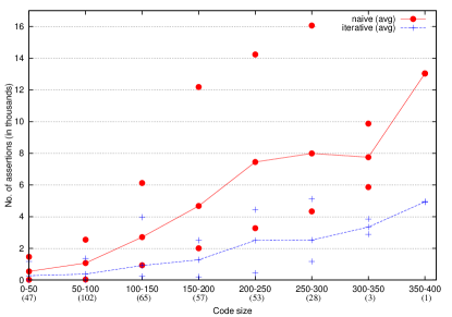
Figure 4: Maximum, average, and minimum number of typing assertions for computing a minimum error source by naive and iterative approach

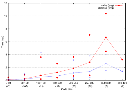
Figure 5: Maximum, average, and minimum execution times for computing a minimum error source by naive and iterative approach

The statistics for execution times are shown in Figure 5. The iterative algorithm is consistently faster than the naive solution. We believe this to be a direct consequence of the fact that our algorithm generates a substantially smaller number of typing constraints. The difference in execution times between our algorithm and the naive approach increases with the size of the input program. Note that the total times shown are collected across all iterations.

We also measured the statistics on the number of iterations and expansions taken by our algorithm. The number of expansions corresponds to the total number of usage locations of let variables that have been expanded in the last iteration of our algorithm. The results, shown in Table 1, indicate that the total number of iterations required does not substantially change with the input size. We hypothesize that this is due to the fact that type errors are usually tied only to a small portion of the input program, whereas the rest of the program is not relevant to the error.

	iterations			expansions
	min	avg	max	min	avg	max
0-50	0	0.49	2	0	1.7	11
50-100	0	0.29	3	0	0.88	13
100-150	0	0.49	4	0	1.37	32
150-200	0	0.44	3	0	1.82	19
200-250	0	0.49	2	0	3.11	30
250-300	0	0.36	2	0	6.04	45
300-350	0	0.67	2	0	3.33	10
350-400	0	0	0	0	0	0

Table 1: Statistics for the number of expansions and iterations when computing a single minimum error source

It is worth noting that both the naive and iterative algorithm compute single error sources. The algorithms may compute different solutions for the same input since the fixed cost function does not enforce unique solutions. The iterative algorithm does not attempt to find a minimum error source in the least number of iterations possible, but rather it expands let definitions on-demand as they occur in the computed error sources. This means that the algorithm sometimes continues expanding let definitions even though there exists a proper minimum error source for the current expansion. In our future work, we plan to consider how to enforce the search algorithm so that it first finds those minimum error sources that require less iterations and expansions.

GRASShopper benchmarks.

We repeated the previous experiments on the generated GRASShopper benchmarks. The benchmarks are grouped by code size. There are four groups of five programs corresponding to programs with 1000, 1500, 2000, and 2500 lines.

Figure 6 shows the total number of generated typing assertions subject to the code size. This figure follows the conventions of Fig. 4 except that the number of constraints is given on a logarithmic scale. The total number of assertions generated by our algorithm is consistently an order of magnitude smaller than when using the naive approach. The naive approach expands all let defined variables where the iterative approach expands only those let definitions that are needed to find the minimum error source. Consequently, the times taken by our algorithm to compute a minimum error source are smaller than when using the naive one, as shown in Figure 7. Beside solving a larger weighed MaxSMT instance, the naive approach also has to spend more time generating typing assertions than our iterative algorithm. Finally, Table 2 shows the statistics on the number of iterations and expansion our algorithm made while computing the minimum error source. Again, the total number of iterations appears to be independent of the size of the input program.

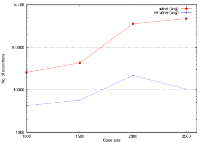
Figure 6: Maximum, average, and minimum number of typing assertions for computing a minimum error source by naive and iterative approach for larger programs

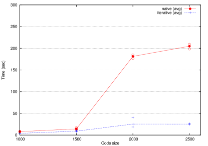
Figure 7: Maximum, average, and minimum execution times for computing a minimum error source by naive and iterative approach for larger programs

	iterations			expansions
	min	avg	max	min	avg	max
1000	0	0.2	1	0	0.2	1
1500	0	0.4	2	0	2.8	14
2000	0	0.6	2	0	53.8	210
2500	0	0.2	1	0	3	15

Table 2: Statistics for the number of expansions and iterations when computing a single minimum error source for larger programs

Comparison to other tools.

Our algorithm also outperforms the approach by Myers and Zhang [33] in terms of speed on the same student benchmarks. While our algorithm ran always under $5$ seconds, their algorithm took over $80$ seconds for some programs. We also ran their tool SHErrLoc [29] on one of our GRASSHopper benchmark programs of $2000$ lines of code. After approximately $3$ minutes, their tool ran out of memory. We believe this is due to the exponential explosion in the number of typing constraints due to polymorphism. For that particular program, the total number of typing constraints their tool generated was roughly $200,000$. On the other hand, their tool shows high precision in correctly pinpointing the actual source of type errors. These results nicely exemplify the nature of type error localization. In order to solve the problem of producing high quality type error reports, one needs to consider the whole typing data. However, the size of that data can be impractically large, making the generation of type error reports slow to the point of being not usable. One benefit of our approach is that these two problems can be studied independently. In this work, we focused on the second problem, i.e., how to make the search for high-quality type error sources practically fast.

6 Conclusion

We have presented a new algorithm that efficiently finds optimal type error sources subject to generic usefulness criteria. The algorithm uses SMT techniques to deal with the large search space of potential error sources, and principal types to abstract the typing constraints of polymorphic functions. The principal types are lazily expanded to the actual typing constraints whenever a candidate error source involves a polymorphic function. This technique avoids the exponential-time behavior that is inherent to type checking in the presence of polymorphic functions and still guarantees the optimality of the computed type error sources. We experimentally showed that our algorithm scales to programs of realistic size. To our knowledge, this is the first type error localization algorithm that guarantees optimal solutions and is fast enough to be usable in practice.

Acknowledgments

This work was in part supported by the National Science Foundation under grant CCF-1350574 and the European Research Council under the European Union’s Seventh Framework Programme (FP/2007-2013) / ERC Grant Agreement nr. 306595 “STATOR”.

References

- [1] A. Aiken and E. L. Wimmers. Type inclusion constraints and type inference. In FPCA, pages 31–41. ACM, 1993.
- [2] C. Barrett, R. Sebastiani, S. A. Seshia, and C. Tinelli. Satisfiability Modulo Theories, chapter 26, pages 825–885. Volume 185 of Biere et al. [5], February 2009.
- [3] C. Barrett, I. Shikanian, and C. Tinelli. An abstract decision procedure for a theory of inductive data types. Journal on Satisfiability, Boolean Modeling and Computation, 3:21–46, 2007.
- [4] C. Barrett, A. Stump, and C. Tinelli. The SMT-LIB standard – version 2.0. In SMT, 2010.
- [5] A. Biere, M. J. H. Heule, H. van Maaren, and T. Walsh, editors. Handbook of Satisfiability, volume 185 of Frontiers in Artificial Intelligence and Applications. IOS Press, February 2009.
- [6] N. Bjørner and A. Phan. Z: Maximal Satisfaction with Z3. In SCSS, 2014.
- [7] N. Bjørner, A. Phan, and L. Fleckenstein. Z: An Optimizing SMT Solver. In TACAS, 2015.
- [8] S. Chen and M. Erwig. Counter-factual typing for debugging type errors. In POPL, pages 583–594. ACM, 2014.
- [9] O. Chitil. Compositional explanation of types and algorithmic debugging of type errors. In ICFP, ICFP ’01, pages 193–204. ACM, 2001.
- [10] L. Damas and R. Milner. Principal type-schemes for functional programs. In POPL, pages 207–212. ACM, 1982.
- [11] L. De Moura and N. Bjørner. Z3: An Efficient SMT Solver. In TACAS, pages 337–340. Springer-Verlag, 2008.
- [12] D. Duggan and F. Bent. Explaining type inference. In Science of Computer Programming, pages 37–83, 1995.
- [13] EasyOCaml. http://easyocaml.forge.ocamlcore.org. [Online; accessed 16-April-2015].
- [14] H. Gast. Explaining ML type errors by data flows. In Implementation and Application of Functional Languages, pages 72–89. Springer, 2005.
- [15] C. Haack and J. B. Wells. Type error slicing in implicitly typed higher-order languages. Sci. Comput. Program., pages 189–224, 2004.
- [16] A. J. Kfoury, J. Tiuryn, and P. Urzyczyn. ML Typability is DEXTIME-Complete. In CAAP, pages 206–220, 1990.
- [17] B. Lerner, M. Flower, D. Grossman, and C. Chambers. Searching for type-error messages. In PLDI. ACM Press, 2007.
- [18] C. M. Li and F. Manyà. MaxSAT, Hard and Soft Constraints, chapter 19, pages 613–631. Volume 185 of Biere et al. [5], February 2009.
- [19] H. G. Mairson. Deciding ML Typability is Complete for Deterministic Exponential Time. In POPL, pages 382–401, 1990.
- [20] N. Narodytska and F. Bacchus. Maximum satisfiability using core-guided maxsat resolution. In Twenty-Eighth AAAI Conference on Artificial Intelligence, 2014.
- [21] M. Neubauer and P. Thiemann. Discriminative sum types locate the source of type errors. In ICFP, pages 15–26. ACM Press, 2003.
- [22] OCaml. http://ocaml.org. [Online; accessed 15-April-2015].
- [23] M. Odersky, M. Sulzmann, and M. Wehr. Type inference with constrained types. TAPOS, 5(1):35–55, 1999.
- [24] Z. Pavlinovic, T. King, and T. Wies. Finding minimum type error sources. In OOPSLA, pages 525–542, 2014.
- [25] Z. Pavlinovic, T. King, and T. Wies. On practical smt-based type error localization. Technical Report TR2015-972, New York University, 2015.
- [26] B. C. Pierce. Types and programming languages. MIT press, 2002.
- [27] R. Piskac, T. Wies, and D. Zufferey. Grasshopper. In Tools and Algorithms for the Construction and Analysis of Systems, pages 124–139. Springer, 2014.
- [28] J. A. Robinson. Computational logic: The unification computation. Machine intelligence, 6(63-72):10–1, 1971.
- [29] SHErrLoc. http://www.cs.cornell.edu/projects/sherrloc/. [Online; accessed 22-April-2015].
- [30] M. Sulzmann, M. Müller, and C. Zenger. Hindley/Milner style type systems in constraint form. Res. Rep. ACRC-99-009, University of South Australia, School of Computer and Information Science. July, 1999.
- [31] F. Tip and T. B. Dinesh. A slicing-based approach for locating type errors. ACM Trans. Softw. Eng. Methodol., pages 5–55, 2001.
- [32] M. Wand. Finding the source of type errors. In POPL, pages 38–43. ACM, 1986.
- [33] D. Zhang and A. C. Myers. Toward general diagnosis of static errors. In POPL, pages 569–581. ACM, 2014.
- [34] D. Zhang, A. C. Myers, D. Vytiniotis, and S. L. P. Jones. Diagnosing type errors with class. In PLDI, pages 12–21, 2015.