Deforming regular black holes

Abstract

In this work we have deformed regular black holes which possess a general mass term described by a function which generalizes the Bardeen and Hayward mass functions. By using linear constraints in the energy-momentum tensor to generate metrics, the solutions presented in this work are either regular or singular. That is, within this approach, it is possible to generate regular or singular black holes from regular or singular black holes. Moreover, contrary to the Bardeen and Hayward regular solutions, the deformed regular black holes may violate the weak energy condition despite the presence of the spherical symmetry. Some comments on accretion of deformed black holes in cosmological scenarios are made.

I Introduction

The existence of singularities is an open and interesting problem in both General Relativity (GR) and other theories of gravity. There is a common belief that only a complete Quantum Theory of Gravity will solve this problem. But without a fully developed candidate for a Quantum Theory of Gravity, the singularities are avoided, for example, with some violations in the energy conditions. And these violations are more acceptable with the observation of cosmic acceleration Supernova ; Supernova2 . By assuming these violations, the Hawking-Penrose theorems are not valid. In cosmology Novello or black hole (BH) physics Joshi , we can create solutions of the gravitational field equations without a singularity. Such solutions may violate the important theorems of Hawking-Penrose and avoid the problem of singularities.

In Bardeen Bardeen2 , one has the first regular black hole (RBH): a compact object with an event horizon and without a physical singularity (see Ansoldi for a review and Lemos_Zanchin for a short introduction). This realization is a consequence of ideas from Sakharov and others Sakharov ; Gliner that the spacetime inside the horizon, where the matter has a high pressure, is de Sitter-like. The Bardeen solution is spherically symmetric and does not violate the weak energy condition (WEC). According to Beato , it is formed by a nonlinear electrodynamic field. Decades later, Hayward Hayward constructed another regular solution with this symmetry. On the other hand, recently, solutions with axial symmetry (BHs with rotation) have been developed as well Various_axial ; Various_axial2 ; Various_axial3 ; Various_axial4 ; Various_axial5 ; Neves_Saa . In our work Neves_Saa , we have constructed a general class of regular solutions using the mass term

$$m(r)=\frac{M_{0}}{\left[1+\left(\frac{r_{0}}{r}\right)^{q}\right]^{p/q}},$$ (1)

where $M_{0}$ and $r_{0}$ are, respectively, mass and length parameters. To accommodate event horizon(s), one adopts $r_{0}\ll M_{0}$ in (1). The Bardeen and Hayward BHs correspond to $p=3,q=2$ and $p=3,q=3,$ respectively. Our solution generalizes previous works because adopts the cosmological constant, axial symmetry and the general mass term (1). Moreover, we show that the WEC is always violated when the rotation is present.

A general approach to build solutions in GR and brane world contexts using linear constraints in the energy-momentum tensor is presented in Molina . From known solutions (such as Schwarzschild, Reissner-Nordström etc.) it is possible to construct metrics deforming the standard solutions. According to the constraint, it is possible to obtain either regular or singular black holes, naked singularities and wormholes. This approach generalizes results from refs. Molina2 ; Casadio ; Bronnikov ; Various ; Various2 ; Various3 (such an approach has been useful to generate spherical RBHs in a brane world. But, in the axial case, RBHs with rotation need another strategy. For example, by using the Kerr-Schild ansatz Various4 ; Neves ). In this work, we shall adopt this procedure to construct solutions from the regular metric presented in Neves_Saa . That is, our ansatz will have the mass term given by eq. (1). Then we shall show that from a regular BH is possible to obtain regular and singular BHs as well.

The structure of this paper is as follows: in Section 2 we present the general features of RBHs with spherical symmetry; in Section 3 we show the general approach to build solutions; in Section 4 we apply this approach by using a general mass term; in Section 5 we investigate the WEC violation; in Section 6 some comments on BHs in cosmological scenarios are made; in Section 7 the final remarks are presented.

In this work, we have used the metric signature $diag(-+++)$ and the geometric units $G=c=1$, where $G$ is the gravitational constant, and $c$ is the speed of light in vacuum.

II General features of spherical regular black holes

According to Neves_Saa , in eq. (1), the only feasible value of $p$ is 3. That is, by adopting $p=3$, the metrics with the mass function (1), in the limit of small $r$, are de Sitter-like (this result agrees with the comments made in Introduction on the interior region of RBHs, where there is a de Sitter core). The mass term function (1) may be written for small and large $r$, respectively, as

$$m(r) \approx M_{0}\left(\frac{r}{r_{0}}\right)^{3},$$ (2)

$$m(r) \approx M_{0}\left(1-\frac{3}{q}\left(\frac{r_{0}}{r}\right)^{q}\right).$$ (3)

It is worth noting that for small $r$, the mass function does not depend on $q$. These approximations will be useful in the next sections.

A family of RBHs with spherical symmetry,

$$ds^{2}=-A(r)dt^{2}+\frac{1}{B(r)}dr^{2}+r^{2}d\Omega^{2},$$ (4)

where $d\Omega^{2}=d\theta^{2}+sin^{2}\theta d\phi^{2},$ may be written by using the mass function (1). These metrics are not vacuum solutions of the gravitational field equations. The energy-momentum tensor, when $A(r)=B(r)=1-2m(r)/r$, is given by

$$T_{\nu}^{\mu}=\frac{1}{8\pi}\left(\begin{array}[]{cccc}-\frac{2m^{\prime}(r)}{r^{2}}\\ &-\frac{2m^{\prime}(r)}{r^{2}}\\ &&-\frac{m^{\prime\prime}(r)}{r}\\ &&&-\frac{m^{\prime\prime}(r)}{r}\end{array}\right),$$ (5)

(the symbol (’) represents an ordinary derivative with respect to $r$). For a general mass function $m(r)$—with the energy-momentum tensor in the form $T_{\nu}^{\mu}=diag\left(-\rho,p_{r},p_{t,}p_{t}\right)$, where $\rho,p_{r}$, and $p_{t}$ are the energy density, radial pressure and tangential pressure, respectively—these metrics are neither isotropic ($p_{r}=p_{t}$) nor have a traceless energy-momentum tensor $(T_{\mu}^{\mu}=0)$.

The standard RBHs (Bardeen and Hayward) do not violate the WEC. That is, $\rho\geq 0$ and $\rho+p_{i}\geq 0$, for $i=r$ and $i=t$, in these metrics. In these solutions, $A(r)=B(r)$ leads to $\rho+p_{r}=0$, $\rho=m^{\prime}(r)/(4\pi r^{2})$ and $\rho+p_{t}=(2m^{\prime}(r)-rm^{\prime\prime}(r))/(8\pi r^{2})$, which are positive definite. However, as we shall see, when $A(r)\neq B(r)$ this is not the case. And WEC violations are possible even in the spherical case. On the other hand, as we have shown in Neves_Saa , the WEC violations are always present for RBHs in the axial case.

The standard Bardeen and Hayward metrics are regular, i.e., the scalars are finite everywhere. For example, for $r\rightarrow 0$, the Bardeen and Hayward black holes have the Kretschmann scalar written as

$$\lim_{r\rightarrow 0}K(r)=\lim_{r\rightarrow 0}R_{\mu\nu\alpha\beta}R^{\mu\nu\alpha\beta}=96\left(\frac{M_{0}}{r_{0}^{3}}\right)^{2},$$ (6)

by using the notation of eq. (1), where this limit is valid for any $q$ positive integer.

In general, a metric in the form (4) has horizons given by zeros of $A(r)$ and $B(r).$ Killing horizons are zeros of $A(r),$ and event horizons are roots of $B(r)$. With the mass term (1), RBHs present an outer horizon (the event horizon), $r_{+},$ and an inner horizon, $r_{-}$, which are Killing horizons, $r_{k}$, only when $A(r)=B(r)$. A static region is present outside of the event horizon when $A(r)>0$ and $B(r)>0,$ where the Killing vector field $\xi_{t}=\frac{\partial}{\partial t}$ is timelike.

III The approach: deforming black holes

In Molina it is showed how to construct solutions in GR by means of deformations. By using a linear constraint in the energy-momentum tensor, it is possible to obtain solutions which are deformations of the vacuum (or electrovacuum) standard solutions (Schwarzschild, Kerr, Reissner-Nordström etc) or standard RBHs. With the assumption that the field equations are

$$R_{\nu}^{\mu}-\frac{1}{2}R\delta_{\nu}^{\mu}=8\pi T_{\nu}^{\mu},$$ (7)

the approach works in the brane world context as well Casadio ; Bronnikov ; Various ; Various2 ; Various3 ; Lobo . In that context, by assuming vacuum on the brane, the "electrical" part of the five-dimensional Weyl tensor projected on the brane is interpreted as a traceless energy-momentum tensor: $E_{\mu\nu}=8\pi T_{\mu\nu}$, with $E_{\mu}^{\mu}=0.$ Thus, in the brane world, the constraint, from (7), is

$$R=0.$$ (8)

Following the work Molina , in GR context, we choose an isotropic constraint as well:

$$p_{r}=p_{t},$$ (9)

which is important, for example, to build BH solutions in cosmological scenarios (see Martin-Moruno ; Neves2 ). Another constraint in GR is given by

$$p_{r}=\omega\rho.$$ (10)

The constraint expressed in (10) was used to build wormhole solutions in Lobo . That is, the components of the energy-momentum tensor, $T^{\mu}_{\nu}=diag(-\rho,p_{r},p_{t},p_{t})$, obey a linear constraint:

$$L(\rho,p_{r},p_{t})\equiv\alpha\rho+\beta p_{r}+2\gamma p_{t}=0.$$ (11)

The constraint (8) corresponds to $\alpha=-1,\beta=1$ and $\gamma=1.$ The isotropic case—constraint (9)—is given by $\alpha=0,\beta=1$ and $\gamma=-1/2,$ and the constraint (10) is equivalent to $\alpha=\omega,\beta=-1$ and $\gamma=0$ in (11).

By using the linear constraint (11) in the field equations (7), with aid of the metric (4), one has

$$\left(\frac{\alpha-\beta}{r^{2}}\right)\left[1-B(r)\right]+\frac{\gamma}{2}\left[\frac{A^{\prime}(r)B^{\prime}(r)}{A(r)}-\left(\frac{A^{\prime}(r)}{A(r)}\right)^{2}\right]+\left(\frac{\beta+\gamma}{r}\right)\left[\frac{B(r)A^{\prime}(r)}{A(r)}\right]-\left(\frac{\alpha-\gamma}{r}\right)B^{\prime}(r)+\gamma\frac{A^{\prime\prime}(r)B(r)}{A(r)}=0.$$ (12)

The general equation (12) will be used to determine the elements of the metric given by eq. (4).

Deformation means: to obtain a set of solutions "close" to the known solutions. By choosing a function $A(r)=A_{0}(r)$, the approach yields to a function $B(r)$ derived from the standard case where $B(r)=A(r)$ in (4). The deformation is applied on the $B(r)$ component because its roots give, for example, the spacetime structure (event horizons when metric is written as eq. (4) and the physical singularity). Then, one seeks for new solutions, according to the spacetime structure, when one deforms the metric (4). In this work, we deal with deformations from the regular metric where

$$A(r)=A_{0}(r)=1-\frac{2m(r)}{r},$$ (13)

with $m(r)$ given by eq. (1) (or (2) and (3)). The ansatz is completed by

$$B(r)=A_{0}(r)+\left(C-1\right)B_{lin}(r),$$ (14)

where $B_{lin}(r)$ stands for the linear term of $B(r)$. The constant $C$ determines the type of solutions: for $C>0$ one has either regular or singular black holes, or naked singularities, $C<0$ (or $C<C_{0}$) may determine wormholes, and for $C=C_{0}$ one has extremal black holes. For $C=1$ the standard cases are restored.

The function $B_{lin}(r)$ is determined from

$$B_{lin}(r)=A_{0}(r)\ exp\left[k\int\frac{dr}{rh(r)}\right],$$ (15)

which is solution of eq. (12) by using the ansatz (13)-(14), where

$$h(r)=\left(\gamma-\alpha\right)A_{0}(r)+\frac{\gamma}{2}rA_{0}^{\prime}(r).$$ (16)

The constant $k$ is $-1$ when $p_{r}=p_{t}$, $k=-2$ when $R=0$, and $k=\omega+1$ when $p_{r}=\omega\rho$.

It is useful using the mass (2) and (3) to solve (15). Then, with the mass approximation for small $r$, eq. (15) reads

$$B_{lin}^{small}(r)=A_{0}(r)\left[\frac{r}{\left(2M_{0}(\alpha-2\gamma)r^{2}-(\alpha-\gamma)r_{0}^{3}\right)^{\frac{1}{2}}}\right]^{\left(\frac{k}{\gamma-\alpha}\right)}.$$ (17)

The denominator of (17) is $h(r)r_{0}^{3}$. On the other hand, for large $r$, we use rational functions for any $q>0$ to solve $B_{lin}(r)$, i.e.,

$$B_{lin}^{large}(r)=A_{0}(r)\prod_{n=1}^{q+1}\frac{1}{|r-r_{n}|^{\left(\frac{kc_{n}}{\alpha-\gamma}\right)}},$$ (18)

with

$$c_{n}=r_{n}^{q}\ \prod_{i=n+1}^{q+1}\prod_{\stackrel{{\scriptstyle j=1}}{{\stackrel{{\scriptstyle 0<j<n}}{{}}}}}^{n-1}\frac{1}{\left(r_{n}-r_{i}\right)\left(r_{n}-r_{j}\right)}.$$ (19)

The $r_{n}$ are the roots of $h(r)$. In general, $h(r)$ has $q+1$ roots, using the mass function (3) and since $(q-1)\gamma+2\alpha\neq 0$. In the regime that we shall adopt henceforth, $q=2$ and $q=3$ (Bardeen and Hayward solutions, respectively), this function has two positive real roots, $r_{0-}<r_{0+}$.

In the next section, we shall use a regular ansatz to construct/deform solutions.

IV Deforming a regular black hole

Because of the regularity of $A_{0}(r)$, we shall focus on $B_{lin}(r)$. The ansatz in this paper has the form (13) with $p=3$ in the mass function. Due to the length or to the cumbersome expressions, the functions $B_{lin}(r)$ (for either small or large $r^{\prime}s$) shown below were obtained by using eqs. (2) and (3). However, in the Figures, we have used $m(r)$ given by (1) to generate $B(r)$.

IV.1 Isotropic case, $p_{r}=p_{t}$

When $\alpha=0,\beta=1,$ $\gamma=-1/2$, and $k=-1$, the eq. (17) admits the following solution for small $r$:

$$B_{lin}^{small}(r)=\frac{A_{0}(r)\ r^{2}}{\left(2M_{0}r^{2}-\frac{r_{0}^{3}}{2}\right)}.$$ (20)

This function diverges at $r=r_{0-}=\frac{1}{2}\sqrt{r_{0}^{3}/M_{0}}$, which corresponds to the smaller positive real root of $h(r)$. Thus, for $C\neq 1,$ all metrics diverge, and the Kretschmann scalar simply reads

$$K\sim\frac{1}{\left(4M_{0}r^{2}-r_{0}^{3}\right)^{4}}.$$ (21)

This result is valid for any value of $C\neq 1$ in (14) for the isotropic case. On the other hand, $B(r)$ and $K$ do not diverge at $r=r_{0+}$ (the largest positive real root of $h(r)$) because the value of $c_{0+}$ is positive in (18).

To study the spacetime structure, we need to know the localization of the event and Killing horizons. The latter correspond to solutions of $A_{0}(r_{k_{i}})=0$, and the inner and the outer horizon (an event horizon) are located at $r_{-}$ and $r_{+}$, respectively, which are roots of $B(r_{\pm})=0$. According to the value of $C$, the number of zeros of $B(r)$ is different (see Fig. 1). In general, assuming the existence of a static region, $A(r)$ and $B(r)$ must be positive definite for $r>r_{+}.$ Therefore, this assumption eliminates values of $C\leq 0.$

For $C>1$ the function $B(r)$ has two zeros, $r_{-}<r_{+}$. The largest zero corresponds to the event horizon $r_{+}$. The metric is singular at $r=r_{0-}<r_{-}$. Then, the spacetime structure reads

$$r_{0-}<r_{-}=r_{k_{1}}<r_{+}=r_{k_{2}}<\infty.$$ (22)

This case corresponds to the singular BH in a noncompact universe, such as presented in Molina2 , which uses the same ansatz but with $m$ constant (our value of $C$ corresponds to the $C+1$ in the cited article).

When $0<C<1$ the situation is quite different: there are three zeros in $B(r)$ (the third zero is not zero of $A(r)$). There is a maximum value of $r$ $(r_{max}>r_{+})$. Such as Molina2 , these values of $C$ lead to a singular BH in a compact universe. The spacetime structure is given by

$$r_{0-}<r_{-}=r_{k_{1}}<r_{+}=r_{k_{2}}<r_{max},$$ (23)

with

$$\lim_{C\rightarrow 1}r_{max}=\infty.$$ (24)

These results are the same of ref. Molina2 . The difference is the localization of the physical singularity: with the mass function (1) or (2), the singularity is translated to $r=r_{0-}$. Unfortunately the ansatz (13) does not prevent the occurrence of the physical singularity for the isotropic deformed geometries $(C\neq 1)$.

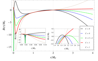
Figure 1: $B(r)$ obtained with the mass function (1) and the constraint $p_{r}=p_{t}$. The vertical dashed line corresponds to the event horizon $r_{+}$. In this graphic we have used $r_{0}/M_{0}=0.1$, $q=3$, $C=-1$, $C=0.5$, and $C=2$.

IV.2 Brane world or traceless energy-momentum tensor, $R=0$

When $\alpha=-1,\beta=1,\gamma=1,$ and $k=-2$, the constraint $R=0$, for small $r$, admits the following solution for (17):

$$B_{lin}^{small}(r)=\frac{A_{0}(r)}{r}\sqrt{-6M_{0}r^{2}+2r_{0}^{3}}.$$ (25)

$B_{lin}^{small}(r)$ diverges only at $r=0$. However, there is a singular point for large $r$. That is, the function $h(r)$ has a root $r_{0+}$ and the exponent $kc_{0+}/(\alpha-\gamma)$, in eq. (18), is positive. Therefore, $B(r)$ diverges at this point (see Fig. 2). Typically, $r_{0+}\approx 3M_{0}/2.$ This point may indicate the physical singularity depending on the value of $C$. Then, in the case $C\neq 1,$ the Kretschmann scalar will read

$$K(r)\sim\frac{1}{\left(r-r_{0+}\right)^{4}}.$$ (26)

The family of solutions generated from the regular ansatz (13) in the case where $R=0$ has the same behaviour illustrated in Casadio ; Bronnikov . Again, when $C>1$ we have singular BHs, where the physical singularity is located at $r_{0+}$; $C=C_{0}$ fixes the extremal case, the root $r=r_{+}$ is double; and $C<C_{0}$ generates a wormhole, with $r_{thr}$ indicating the throat of the hole. Lastly, the case $C_{0}<C<1$ presents a regular black hole, where there is a minimum value of $r=r_{min}$: this point is the end of the spacetime, and the Kretschmann scalar is always finite because $r_{min}>r_{0+}$. The latter two cases ($C<C_{0}$ and $C_{0}<C<1$) are possible because $B(r)$ has a second root.

For $C>1$ and $C=C_{0}$, the spacetime structure is given by

$$r_{0+}<r_{k}=r_{+}<\infty.$$ (27)

When $C<C_{0},$ the radial coordinate assumes $[r_{thr},\infty[$, i.e., the second root of $B(r)$ in this case is $r_{thr}>r_{k}$, and the spacetime is static only when $r\geq r_{thr}$. The spacetime structure in the single regular case $C_{0}<C<1$ reads

$$r_{min}<r_{k}=r_{+}<\infty.$$ (28)

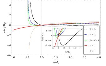
Figure 2: $B(r)$ obtained with the mass function (1) and the constraint $R=0$. The vertical dashed line corresponds to the event horizon $r_{+}$. In this graphic we have used $r_{0}/M_{0}=0.1$, $q=3$, $C=-1$, $C_{0}=0.5$, $C=0.8$, and $C=2$.

IV.3 Constraint $p_{r}=\omega\rho$

When $\alpha=\omega,\beta=-1,\gamma=0$ and $k=\omega+1$, the function $h(r)$ is quite simple, by using the mass function (1) or (2)-(3). In this case, $h(r)=-\omega A(r)$, and the divergence of $B(r),$ for the deformed metrics, occurs in either $r=r_{0-}=r_{k_{1}}$ or $r=r_{0+}=r_{k_{2}}$. For large $r$, one has

$$B_{lin}^{large}(r)\sim\frac{1}{|r-r_{k_{2}}|^{\left(c_{0+}\left(\frac{1+\omega}{\omega}\right)-1\right)}},$$ (29)

with $c_{0+}\approx 1$ (the minus one in the exponent comes from $A_{0}(r)\sim(r-r_{k_{2}})$). Then, the divergence of $B(r)$ in $r=r_{k_{2}}$ depends on the sign of $\omega.$ But the divergence of the Kretschmann scalar in this point, due to the existence of this root for $h(r),$ is not given by the divergence of $B(r).$ The Kretschmann scalar reads

$$K(r)\sim\frac{\left(\left(1+\omega\right)c_{0+}\right)^{2}}{\omega^{2}(r-r_{k_{2}})^{2\left(1+\left(\frac{1+\omega}{\omega}\right)c_{0+}\right)}}.$$ (30)

Therefore, this metric has a physical singularity at $r_{k_{2}}$ when $(1+\left(\frac{1+\omega}{\omega}\right)c_{0+})>0$ $(\omega>0$ or $\omega<-c_{0+}/(1+c_{0+}))$. The behaviour of $B(r)$ in this case is shown in Fig. 3 (left). For $C>1$, we have a naked singularity. There is no event horizon or, equivalently, a root of $B(r)$ in such a spacetime. With $C<1,$ the geometries are described by wormholes. There is a large root for $B(r_{thr})$ such that $r_{thr}>r_{0+}=r_{k_{2}}$, and the metric signature is incorrect for $r<r_{thr}$. Thus, for $(1+\left(\frac{1+\omega}{\omega}\right)c_{0+})>0,$ the physical solutions considered here are the standard solution $(C=1)$, naked singularities $(C>1)$ and wormholes $(C<1)$.

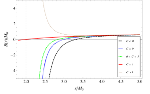
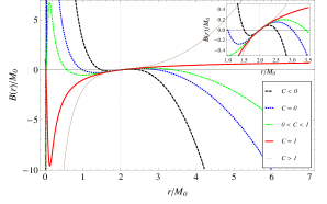
Figure 3: Left: $B(r)$ obtained with the mass function (1) and the constraint $p_{r}=\omega\rho$ for $\omega>0$ or $\omega<-c_{0+}/(1+c_{0+})$. Right: the same function for $-c_{0+}/(1+c_{0+})\leq\omega<0$. The vertical dashed line corresponds to the event horizon $r_{+}$. In this graphic we have used $r_{0}/M_{0}=1,$ $q=3$, $\omega=1/3$ (left), $\omega=-1/3$ (right), $C=-2$, $C=0.5$, and $C=2$.

With $-c_{0+}/(1+c_{0+})\leq\omega<0$, the divergence of $B(r)$ and $K(r)$ occurs at $r=r_{0-}$ for the deformed metrics. $B_{lin}^{small}(r)$, by using (17), reads

$$B_{lin}^{small}(r)=\frac{A_{0}(r)}{r^{\left(\frac{1+\omega}{\omega}\right)}}\left[\omega(2M_{0}r^{2}-r_{0}^{3})\right]^{\frac{1}{2}\left(\frac{1+\omega}{\omega}\right)}.$$ (31)

Thus, $r_{0-}=\sqrt{r_{0}^{3}/(2M_{0})}$. In the Fig. 3 (right), by fixing $C>1$, one has a singular BH. In this range of $\omega,$ the values of $C$ which correspond to the physical solutions with correct metric signature are $C=1$ and $C>1$.

V Weak energy condition

In general, according to Section 2, RBHs with spherical symmetry do not violate the WEC. The weak violation occurs, as we have shown in Neves_Saa , when the rotation, represented by metrics with axial symmetry, is present. However, the family of deformed spherical solutions, obtained from a regular ansatz in this work, violates the WEC. For example, in the $R=0$ case, for $q=3$, the relations among $\rho$ and $p^{\prime}s$ are

$$\rho+p_{r} \propto \left(C-1\right)\frac{\left(r-r_{+}\right)}{r^{2}\left(r-r_{0+}\right)^{2}},$$ (32)

$$\rho+p_{t} \propto -\frac{\left(C-1\right)}{r^{2}\left(r-r_{0+}\right)^{2}}+\mathcal{O}\left(1/r^{8}\right).$$ (33)

For any $C\neq 1,$ the WEC is always violated (inside or/and outside of the event horizon $\rho+p_{r}<0$ or/and $\rho+p_{t}<0$). This conclusion may be reached if $m(r)=m$ is used (the Schwarzschild metric) in the ansatz (13).

Therefore, in the specific case $R=0$ with $C_{0}<C<1$, one has a RBH with spherical symmetry which violates the WEC. This interesting result is possible only for deformed metrics, i.e., $A(r)\neq B(r)$.

VI Cosmological fluids

It is worth noting that the isotropic case may produce BHs in cosmological scenarios. Such solutions present one of the most important characteristics of the modern cosmology: the isotropy at large scales. Assuming (14) as $B(r)=A_{0}(r)\left[1+(C-1)b(r)\right]$, with $b(r)=exp\left[\int k/(rh(r))dr\right]$, one has

$$\omega(r_{+})=\frac{p(r_{+})}{\rho(r_{+})}=-1,$$ (34)

with $p=p_{r}=p_{t}$ in this case. According to refs. Molina2 ; Martin-Moruno , which used an ansatz with constant mass, $m(r)=m$, this result indicates which deformed BHs do not accrete the fluid with equation of state (34). Such an equation of state is the same of BHs in asymptotically de Sitter geometries. And these geometries do not accrete with such a condition. That is, there is no accretion of the cosmological constant behaving as a fluid. On the other hand, we have shown in Neves_Saa2 that RBHs (non-deformed, i.e., $A(r)=B(r)$) accrete and lost their masses when the test fluid is phantom type, $\omega<-1$. This result is the same obtained with singular BHs (see, for example, Babichev1 ). However, with the mass function (1), the accretion occurs when

$$\left(\frac{r_{0}}{r_{c}}\right)^{q}<\frac{1}{2},$$ (35)

with $r_{c}$ playing the role of a critical point, where the speed of flow is equal to the speed of sound.

VII Final remarks

By employing the approach applied in Molina2 ; Casadio ; Bronnikov ; Various ; Various2 ; Various3 and generalized in Molina , we have deformed RBHs for the first time in the literature. This approach works by means of linear constraints in the energy-momentum tensor. From a known ansatz (a determined geometry such as Schwarzschild, Reissner-Nordström, Bardeen or Hayward solution), it is possible to build metrics which represent different types of solutions: regular or singular black holes, wormholes and naked singularities. In this work, our ansatz was given by a regular metric with a general mass function, proposed by us in Neves_Saa , to construct RBHs with either spherical or axial symmetry. By using this mass function, the spherical deformed geometries presented here are, in general, singular. That is, the standard RBHs used as ansatz (Bardeen and Hayward solutions) avoid the singularity issue, but the deformed metrics derived from them diverge inside the event horizon. However there is an important exception: with $C_{0}<C<1$ in the brane world context (or, equivalently, a traceless energy-momentum tensor in GR context), one has a deformed RBH.

Another important issue studied here was the WEC violation. The standard RBHs with spherical symmetry do not violate the WEC. However, deformed solutions may in general violate this energy condition outside and inside the event horizon, according to eqs. (32)-(33). Therefore, it is possible to obtain a RBH with spherical symmetry (the case $C_{0}<C<1$ above quoted) that violates the WEC.

Lastly, in the isotropic case for the metrics presented in this work, the equation of state of the deformed metrics at the event horizon, eq. (34), indicates the same value when we have an asymptotically de Sitter BH with energy-momentum tensor given by the cosmological constant. These de Sitter-type objects, according to ref. Martin-Moruno , do not accrete a fluid represented by the cosmological constant. The same interpretation is possible for deformed metrics presented here. Moreover, as we can see in (35), the accretion gives a constraint for the value of $q$ in the metric.

- (1) A. G. Riess et al. (Supernova Search Team Collaboration), Observational Evidence from Supernovae for an Accelerating Universe and a Cosmological Constant, Astron. J. 116 (1998) 1009 [arXiv:astro-ph/9805201]
- (2) S. Perlmutter et al. (Supernova Cosmology Project Collaboration), Measurements of Omega and Lambda from 42 High-Redshift Supernovae, Astrophys. J. 517 (1999) 565 [arXiv:astro-ph/9812133]
- (3) M. Novello, S. E. Perez Bergliaffa, Bouncing Cosmologies, Phys. Rept. 463 (2008) 127 [arXiv:0802.1634]
- (4) P. S. Joshi, Spacetime singularities, in Springer Handbook of Spacetime, edited by A. Ashtekar and V. Petkov, Springer-Verlag Berlin Heidelberg (2014), p. 409
- (5) J. M. Bardeen, inConference Proceedings of GR5, Tbilisi, URSS (1968), p. 174
- (6) S. Ansoldi, Spherical black holes with regular center: a review of existing models including a recent realization with Gaussian sources, in Proceedings of BH2, Dynamics and Thermodynamics of Black Holes and Naked Singularities, Milano, Italy, May 2007 [arXiv:0802.0330]
- (7) J. P. S. Lemos and V. T. Zanchin, Regular black holes: Electrically charged solutions, Reissner-Nordström outside a de Sitter core, Phys. Rev. D 83 (2011) 124005 [arXiv:1104.4790]
- (8) A.D. Sakharov, Sov. Phys. JETP 22 (1966) 241
- (9) E.B. Gliner, Sov. Phys. JETP 22 (1966) 378
- (10) E. Ayon-Beato, A. Garcia, The Bardeen Model as a Nonlinear Magnetic Monopole, Phys. Lett. B 493 (2000) 149 [arXiv:gr-qc/0009077]
- (11) S. A. Hayward, Formation and evaporation of non-singular black holes, Phys. Rev. Lett. 96 (2006) 031103 [arXiv:gr-qc/0506126]
- (12) A. Smailagic, E. Spallucci, "Kerrr" black hole: the Lord of the String, Phys. Lett. B 688 (2010) 82 [arXiv:1003.3918]
- (13) L. Modesto, P. Nicolini, Charged rotating noncommutative black holes, Phys. Rev. D 82 (2010) 104035 [ arXiv:1005.5605]
- (14) C. Bambi, L. Modesto, Rotating regular black holes, Phys. Lett. B 721 (2013) 329 [arXiv:1302.6075]
- (15) B. Toshmatov, B. Ahmedov, A. Abdujabbarov, Z. Stuchlik, Rotating Regular Black Hole Solution, Phys. Rev. D 89 (2014) 104017 [arXiv:1404.6443]
- (16) M. Azreg-Ainou, Generating rotating regular black hole solutions without complexification, Phys. Rev. D 90 (2014) 064041 [ arXiv:1405.2569]
- (17) J. C. S. Neves, A. Saa, Regular rotating black holes and the weak energy condition, Phys. Lett. B 734 (2014) 44 [arXiv:1402.2694]
- (18) C. Molina, Deformations of the vacuum solutions of general relativity subjected to linear constraints, Phys. Rev. D 88 (2013) 127501 [arXiv:1311.7137]
- (19) C. Molina, P. Martin-Moruno, P. F. Gonzalez-Diaz, Isotropic extensions of the vacuum solutions in general relativity, Phys. Rev. D 84 (2011) 104013 [arXiv:1107.4627]
- (20) R. Casadio, A. Fabbri, L. Mazzacurati, New black holes in the brane-world?, Phys. Rev. D 65 (2002) 084040 [arXiv:gr-qc/0111072]
- (21) K. A. Bronnikov, S. W. Kim, Possible wormholes in a brane world, Phys. Rev. D 67 (2003) 064027 [arXiv:gr-qc/0212112]
- (22) K. A. Bronnikov, V. N. Melnikov, H. Dehnen, General class of brane-world black holes, Phys. Rev. D 68 (2003) 024025 [arXiv:gr-qc/0304068]
- (23) C. Molina, J. C. S. Neves, Black holes and wormholes in AdS branes, Phys. Rev. D 82 (2010) 044029 [ arXiv:1005.1319]
- (24) C. Molina, J. C. S. Neves, Wormholes in de Sitter branes, Phys. Rev. D 86 (2012) 024015 [arXiv:1204.1291]
- (25) J. C. S. Neves, C. Molina, Rotating black holes in a Randall-Sundrum brane with a cosmological constant, Phys. Rev. D 86 (2012) 124047 [ arXiv:1211.2848]
- (26) J. C. S. Neves, Note on regular black holes in a brane world, Phys. Rev. D 92 (2015) 084015 [arXiv:1508.03615]
- (27) F. S. N. Lobo, A general class of braneworld wormholes, Phys. Rev. D 75 (2007) 064027 [arXiv:gr-qc/0701133]
- (28) P. Martin-Moruno, A. E. Marrakchi, S. Robles-Perez and P. F. Gonzalez-Diaz, Dark Energy Accretion onto black holes in a cosmic scenario, Gen. Rel. Grav. 41 (2009) 2797 [arXiv:0803.2005]
- (29) J. C. S. Neves, Are black holes in an ekpyrotic phase possible?, Astrophys. Space Sci. 361 (2016) 281 [arXiv:1509.03304]
- (30) J. C. S. Neves, A. Saa (in preparation)
- (31) E. Babichev, V. Dokuchaev, Yu. Eroshenko, Black hole mass decreasing due to phantom energy accretion, Phys. Rev. Lett. 93 (2004) 021102 [arXiv:gr-qc/0402089]