Disentangling the excitation conditions of the dense gas in M17 SW

Abstract

Context. Stars are formed in dense molecular clouds. These dense clouds experience radiative feedback from UV photons, and X-ray from stars, embedded pre-stellar cores, YSOs, and ultra compact H II regions. This radiative feedback affects the chemistry and thermodynamics of the gas.

Aims. We aim to probe the chemical and energetic conditions created by radiative feedback through observations of multiple CO, HCN and HCO⁺ transitions. We measure the spatial distribution and excitation of the dense gas ($n(\rm H_{2})>10^{4}\leavevmode\nobreak\ \rm{cm^{-3}}$) in the core region of M17 SW and aim to investigate the influence of UV radiation fields.

Methods. We used the dual band receiver GREAT on board the SOFIA airborne telescope to obtain a 5^′.7$\times$3^′.7 map of the $J=16\rightarrow 15$, $J=12\rightarrow 11$, and $J=11\rightarrow 10$ transitions of ¹²CO in M17 SW. We compare these maps with corresponding APEX and IRAM 30m telescope data for low- and mid-$J$ CO, HCN and HCO⁺ emission lines, including maps of the HCN $J=8\to 7$ and HCO⁺ $J=9\to 8$ transitions. The excitation conditions of ¹²CO, HCO⁺ and HCN are estimated with a two-phase non-LTE radiative transfer model of the line spectral energy distributions (LSEDs) at four selected positions. The energy balance at these positions is also studied.

Results. We obtained extensive LSEDs for the CO, HCN and HCO⁺ molecules toward M17 SW. These LSEDs can be fit simultaneously using the same density and temperature in the two-phase models and to the spectra of all three molecules over a $\sim 12$ square arc minute size region of M17 SW. Temperatures of up to 240 K are found toward the position of the peak emission of the ¹²CO $J=16\to 15$ line. High densities of 10${}^{6}\leavevmode\nobreak\ \rm{cm^{-3}}$ were found at the position of the peak HCN $J=8\to 7$ emission.

Conclusions. We found HCO⁺/HCN line ratios larger than unity, which can be explained by a lower excitation temperature of the higher-$J$ HCN lines. The LSED shape, particularly the high-$J$ tail of the CO lines observed with SOFIA/GREAT, is distinctive for the underlying excitation conditions. The cloudlets associated with the cold component of the models are magnetically subcritical and supervirial at most of the selected positions. The warm cloudlets instead are all supercritical and also supervirial. The critical magnetic field criterion implies that the cold cloudlets at two positions are partially controlled by processes that create and dissipate internal motions. Supersonic but sub-Alfvénic velocities in the cold component at most selected positions indicates that internal motions are likely MHD waves. Magnetic pressure dominates thermal pressure in both gas components at all selected positions, assuming random orientation of the magnetic field. The magnetic pressure of a constant magnetic field throughout all the gas phases can support the total internal pressure of the cold components, but it cannot support the internal pressure of the warm components. If the magnetic field scales as $B\propto n^{2/3}$, then the evolution of the cold cloudlets at two selected positions, and the warm cloudlets at all selected positions, will be determined by ambipolar diffusion.

1 Introduction

Inhomogeneous and clumpy clouds, or a partial face-on illumination in star-forming regions like M17 SW, S106, S140, the Great Nebula portion of the Orion Molecular Cloud, and the NGC 7023 Nebula, produce extended emission of atomic lines like [C I] and [C II], and suppress the stratification in [C II], [C I] and CO emission expected from standard steady-state models of photon-dominated regions (PDRs) (e.g. Keene et al. 1985; Genzel et al. 1988; Stutzki et al. 1988; Gerin & Phillips 1998; Yamamoto et al. 2001; Schneider et al. 2002, 2003; Mookerjea et al. 2003; Pérez-Beaupuits et al. 2010, 2012). The complex line profiles observed in optically thin lines from, e.g., [C I], CS, C¹⁸O, ¹³CO and their velocity-channel maps, are indicative of the clumpy structure of molecular clouds and allow for a robust estimation of their clump mass spectra (e.g. Carr 1987; Loren 1989; Stutzki & Güsten 1990; Hobson 1992; Kramer et al. 1998, 2004; Pérez-Beaupuits et al. 2010). In fact, clumpy PDR models can explain extended [C I] ${}^{3}P_{1}\to{{}^{3}P_{0}}$ emission and a broad LSED for various PDRs and even the whole Milky Way (Stutzki & Güsten 1990; Spaans & van Dishoeck 1997; Cubick et al. 2008; Ossenkopf et al. 2010).

Massive star forming regions like the Omega Nebula M17, with a nearly edge-on view, are ideal sources to study the clumpy structure of molecular clouds, as well as the chemical and thermodynamic effects of the nearby ionizing sources. At a (trigonometric paralax) distance of $\sim$1.98 kpc (Xu et al. 2011), the south-west region of M17 (M17 SW) concentrates molecular material in a clumpy structure. The structure of its neutral and molecular gas appears to be dominated by magnetic rather than by thermal gas pressure, in contrast to many other PDRs (Pellegrini et al. 2007), since magnetic fields as strong as $-700\leavevmode\nobreak\ \mu$G have been measured from H I and OH Zeeman observations (Brogan et al. 1999; Brogan & Troland 2001).

Models based on far-IR and sub-millimeter observations (Stutzki et al. 1988; Meixner et al. 1992) suggest that the distribution and intensity of the emissions observed in the M17 SW complex can be explained with high density ($n(\rm H_{2})\sim 5\times 10^{5}\leavevmode\nobreak\ \rm{cm^{-3}}$) clumps embedded in a less dense interclump medium ($n(\rm H_{2})\sim 3\times 10^{3}\leavevmode\nobreak\ \rm{cm^{-3}}$) surrounded by a diffuse halo ($n(\rm H_{2})\sim 300\leavevmode\nobreak\ \rm{cm^{-3}}$).

More recent results from the Stratospheric Observatory for Infrared Astronomy (SOFIA) and the German REceiver for Astronomy at Terahertz frequencies (GREAT) showed that the line profiles and distribution of the [C II] 158 $\mu$m emission support the clumpy scenario in M17 SW (Pérez-Beaupuits et al. 2012) and that at least 64% of the [C II] 158 $\mu$m emission is not associated with the star-forming material traced by the [C I] and C¹⁸O lines (Pérez-Beaupuits et al. 2013, 2015).

There are more than 100 stars illuminating M17 SW, of which its central cluster is NGC 6618 (e.g. Lada et al. 1991; Hanson et al. 1997). The two components of the massive binary CEN1 (Kleinmann 1973; Chini et al. 1980) are part of this central cluster. This source, originally classified as a double O or early B system by Kleinmann (1973), is actually composed of two O4 visual binary stars with a separation of $\sim 1\aas@@fstack{\prime\prime}8$, named CEN 1a (NE component) and CEN 1b (SW component), and it appears to be the dominant source of photo-ionization in the whole M17 region (Hoffmeister et al. 2008).

The components of the CEN1 binary are also the brightest X-ray sources detected with Chandra in the M17 region (Broos et al. 2007). These Chandra observations, together with a new long ($\sim 300$ ks) exposure of the same field, yielded a combined dataset of $\sim 2000$ X-ray sources, with many of them having a stellar counterpart in IR images. (Townsley et al. 2003; Getman et al. 2010). Although the brightest X-ray sources are CEN 1a and CEN 1b from the central NGC 6618 cluster, other stellar concentrations of $\sim 40$ heavily obscured ($E_{median}\geq 2.5$ keV, $A_{V}>10$ mag) X-ray sources are distributed along the eastern edge of the M17 SW molecular core. The densest concentration of X-ray sources coincides with the well known star-forming region M17-UC1 and the concentration ends around the Kleinmann-Wright Object (Broos et al. 2007, their Fig. 10). The M17-UC1 (G15.04-0.68), an ultracompact H II region first studied by Felli et al. (1980), harbors an ionizing source classified as a B0$-$B0.5 star which, together with its southern companion (IRS 5S), correspond to a massive Class I source with an observable evolution in the MIR and radio wavebands (Chini et al. 2000).

In this study we present maps of multiple high-$J$ transitions of ¹²CO, ¹³CO, HCN and HCO⁺. We analyze the underlying excitation conditions from the LSED of some of the clumps fitted to their spectral lines. We are particularly interested in these molecules because their distribution and excitation is responsive to energetic radiative environments, which has led to their extensive usage for, e.g., disentangling star formation vs. black hole accretion and shocks, in the nuclear region of active galaxies (e.g. Sternberg et al. 1994; Kohno et al. 1999; Kohno & et al. 2001; Kohno 2003, 2005; Usero et al. 2004; Pérez-Beaupuits et al. 2007; García-Burillo et al. 2008; Loenen et al. 2008; Krips et al. 2008; Pérez-Beaupuits et al. 2009; Rosenberg et al. 2014; García-Burillo et al. 2014; Viti et al. 2014)

Given the relative youth ($\lesssim 1$ Myr, e.g. Lada et al. 1991; Hanson et al. 1997) of the main ionizing cluster (NGC 6618) of M17 SW, and the absence of evolved stars, it is likely that supernovae have not yet occurred. This makes M17 SW an ideal place to study the radiative interactions of massive stars with their surrounding gas/dust and stellar disks, without the influence of nearby supernovae. This allows us to study the effects of UV, IR, and X-ray radiation fields on the emission of CO, HCN, and HCO⁺ in a well defined environment.

This study of M17 SW can be considered as one more Galactic template for extra-galactic star forming regions. Therefore, we expect that our results will be important for future high resolution observations where similar regions in extra-galactic sources will be studied in great spatial detail with, e.g., ALMA (Schleicher et al. 2010).

The organization of this article is as follows. In Sect. 2 we describe the observations. The maps of lines observed are presented in Sect. 3. The modeling and analysis of the ambient conditions are presented in Sect. 4. The conclusions and final remarks are presented in Sect. 5.

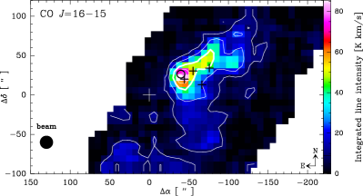
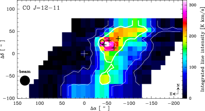
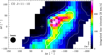
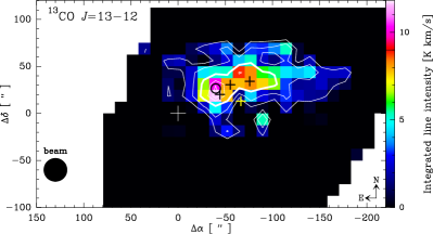
Figure 1: Colour maps of the integrated intensity of the $J=16\to 15$, $J=12\to 11$ and $J=11\to 10$ transitions of ¹²CO, and the ¹³CO $J=13\to 12$ line in M17 SW. The contour levels are the 10%, 25%, 50% (thick line), 75% and 90% of the peak emissions. The central position ($\Delta\alpha=0$, $\Delta\delta=0$), marked with a cross, corresponds to the star SAO 161357 at R.A(J2000)=$18^{h}20^{m}27.6^{s}$ and Dec(J2000)=$-16^{\circ}12\arcmin 00\aas@@fstack{\prime\prime}9$. The ultracompact H II region M17-UC1 and four H₂O masers (Johnson et al. 1998) are marked by the circle and plus symbols, respectively. The ¹³CO $J=13\to 12$ map was convolved with a $25^{\prime\prime}$ beam to match the resolution of the ¹²CO $J=12\to 11$ and to increase the S/N. All pixels with S/N$<3$ (or an rms$>0.22$ K) were blanked in the ¹³CO map.

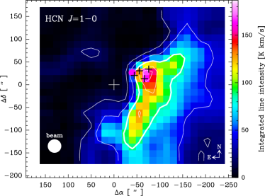
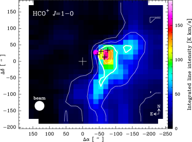
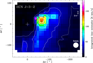
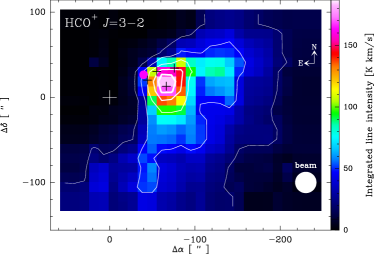
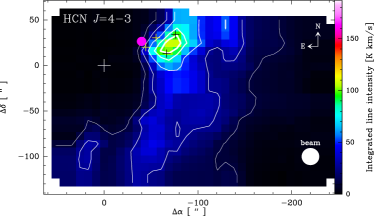
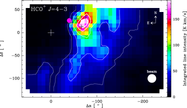
Figure 2: Top panels - Maps of the integrated temperature of the HCN and HCO⁺ $J=1\to 0$ lines in M17 SW. The peak emissions are $\sim$169 ${\rm K}\,{\rm km}\,{\rm s}^{-1}$ and $\sim$152 ${\rm K}\,{\rm km}\,{\rm s}^{-1}$, respectively. The contour levels for all panels in this figure are, from thin to thick, the 10%, 25%, 50%, 75% and 90% of the peak emission. Middle panels - Maps of the integrated temperature of HCN and HCO⁺ $J=3\to 2$ lines, with peak emissions of $\sim$133 ${\rm K}\,{\rm km}\,{\rm s}^{-1}$ and $\sim$183 ${\rm K}\,{\rm km}\,{\rm s}^{-1}$, respectively. Bottom panels - Maps of the integrated temperature of the HCN and HCO⁺ $J=4\to 3$ lines in M17 SW. The peak emissions are $\sim$107 ${\rm K}\,{\rm km}\,{\rm s}^{-1}$ and $\sim$187 ${\rm K}\,{\rm km}\,{\rm s}^{-1}$, respectively. The reference position ($\Delta\alpha=0$, $\Delta\delta=0$) marked with a cross, and other symbols, are as in Fig. 1. The integrated temperature scale is the same in all maps.

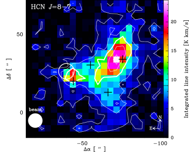
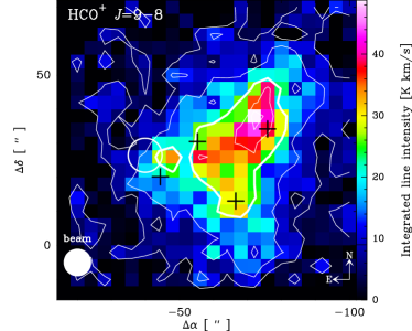
Figure 3: Line intensity maps of the HCN $J=8\to 7$ and HCO⁺ $J=9\to 8$ transitions in the dense core of M17 SW. The contour levels are the 10%, 25%, 50% (thick contour), 75% and 90% of the peak emission. The reference position ($\Delta\alpha=0$, $\Delta\delta=0$) marked with a cross, and other symbols, are as in Fig. 1 and 2.

Table 1: Line parameters of observed transitions.

Transition	$\nu_{0}$	$\theta^{*}_{mb}$	$E_{up}$	$n_{crit}$	Telescope/Instrument
	[GHz]	[′′]	[K]	[$\rm{cm^{-3}}$]
12CO
$J=1\to 0$	115.271	22.6	5.53	2$\times$103	IRAM 30m/EMIR
$J=2\to 1$	230.538	11.3	16.60	7$\times$103	IRAM 30m/EMIR
$J=3\to 2$	345.796	18.9	33.19	2$\times$104	APEX/FLASH+
$J=4\to 3$	461.041	14.1	55.32	4$\times$104	APEX/FLASH+
$J=6\to 5$	691.473	9.6	116.16	1$\times$105	APEX/CHAMP+
$J=7\to 6$	806.652	8.2	154.87	2$\times$105	APEX/CHAMP+
$J=11\to 10$	1267.014	24.2	364.97	8$\times$105	SOFIA/GREAT
$J=12\to 11$	1381.995	22.2	431.29	9$\times$105	SOFIA/GREAT
$J=13\to 12$	1496.923	20.9	503.13	1$\times$106	SOFIA/GREAT
$J=16\to 15$	1841.346	16.6	751.72	2$\times$106	SOFIA/GREAT
13CO
$J=1\to 0$	110.201	23.7	5.29	2$\times$103	IRAM 30m/EMIR
$J=2\to 1$	220.399	11.8	15.87	1$\times$104	IRAM 30m/EMIR
$J=3\to 2$	330.588	19.7	31.73	3$\times$104	APEX/FLASH+
$J=6\to 5$	661.067	10.0	111.05	3$\times$105	APEX/CHAMP+
$J=13\to 12$	1431.153	21.4	481.02	2$\times$106	SOFIA/GREAT
HCN
$J=1\to 0$	88.632	29.4	4.25	2$\times$106	IRAM 30m/EMIR
$J=3\to 2$	265.886	24.9	25.52	1$\times$107	APEX/HET230
$J=4\to 3$	354.505	18.7	42.53	3$\times$107	APEX/FLASH
$J=8\to 7$	708.877	9.2	153.11	2$\times$108	APEX/CHAMP+
H13CN
$J=1\to 0$	86.339	30.2	4.14	2$\times$106	IRAM 30m/EMIR
$J=3\to 2$	259.012	25.2	24.86	5$\times$107	APEX/HET230
$J=4\to 3$	345.339	19.2	41.43	1$\times$108	APEX/FLASH
HCO+
$J=1\to 0$	89.189	29.2	4.28	2$\times$105	IRAM 30m/EMIR
$J=3\to 2$	267.558	24.8	25.68	3$\times$106	APEX/HET230
$J=4\to 3$	356.734	18.6	42.80	6$\times$106	APEX/FLASH
$J=9\to 8$	802.458	8.1	192.58	9$\times$107	APEX/CHAMP+
H13CO+
$J=1\to 0$	86.754	30.1	4.16	2$\times$105	IRAM 30m/EMIR
$J=3\to 2$	260.255	25.1	24.98	3$\times$106	APEX/HET230

2 Observations

2.1 The SOFIA/GREAT data

The new high-$J$ CO observations were performed with the German Receiver for Astronomy at Terahertz Frequencies (GREAT, Heyminck et al. 2012) on board the Stratospheric Observatory For Infrared Astronomy (SOFIA, Young et al. 2012).

We used the dual-color spectrometer during the Cycle-1 flight campaign of 2013 July to simultaneously map a region of about 310${}^{\prime\prime}\times$220^′′ ($\sim$3.0 pc $\times$ 2.1 pc) in the ¹²CO $J=11\rightarrow 10$ at 1381.995105 GHz (216.9 $\mu$m) and the ¹²CO $J=16\rightarrow 15$ transition at 1841.345506 GHz (162.8 $\mu$m) toward M17 SW.

We also present data for the ¹²CO $J=12\rightarrow 11$ transition at 1381.995105 GHz (200.3 $\mu$m) that was mapped during the Early Science flight on 2011 June. Due to lack of time during the observing campaign, the northern map could not be extended beyond $\Delta\delta\sim 70^{\prime\prime}$.

The observations were performed in on-the-fly (OTF) total power mode. The area mapped consists of six strips, each covering $224^{\prime\prime}\times 32^{\prime\prime}$ ($\Delta\alpha\times\Delta\delta$ with a sampling of $8^{\prime\prime}$, half the beamwidth at 1.9 THz. Hence, each strip consists of four OTF lines containing 28 points each. We integrated 1s per dump and 5s for the off-source reference.

All our maps are centered on R.A.(J2000)=$18^{h}20^{m}27.6^{s}$ and Dec(J2000)=$-16^{\circ}12\arcmin 00\aas@@fstack{\prime\prime}9$, which corresponds to the star SAO 161357. For better system stability and higher observing efficiency we used a nearby reference position at offset (345^′′,$-230^{\prime\prime}$). A pointed observation of this reference position against the reference (offset: 1040^′′,$-535^{\prime\prime}$, Matsuhara et al. 1989) showed that the reference is free of ¹²CO emission.

Pointing was established with the SOFIA optical guide cameras, and was accurate to a few arc seconds during Cycle-1 observations. As backends we used the Fast Fourier Transform spectrometers (Klein et al. 2012), which provided 1.5 GHz bandwidth with 212 kHz ($\sim$0.03 ${\rm km\,s}^{-1}$) spectral resolution. The calibration of this data in antenna temperature was performed with the kalibrate task from the kosma_software package (Guan et al. 2012). Using the beam efficiencies ($\eta_{c}$) 0.67 for the ¹²CO $J=16\to 15$, $J=11\to 10$ and ¹³CO $J=13\to 12$ lines, 0.54 for ¹²CO $J=12\to 11$, and the forward efficiency ($\eta_{f}$) of 0.97, we converted all data to main beam brightness temperature scale, $T_{mb}=\eta_{f}\times T_{A}^{*}/\eta_{c}$.

2.2 The APEX data

We have used the lower frequency band of the dual channel DSB receiver FLASH⁺ (Heyminck et al. 2006; Klein et al. 2014) on the Atacama Pathfinder EXperiment 12 m submillimeter telescope (APEX; Güsten et al. 2006) during 2012 November, to map the whole M17 region in the $J=3\to 2$ and $J=4\to 3$ transitions of ¹²CO, as well as the ¹³CO $J=3\to 2$ line. The observed region covers about $6^{\prime}.2\times 7^{\prime}.2$ (4.1 pc $\times$ 4.7 pc). In this work, however, we present only a smaller fraction matching the region mapped with SOFIA/GREAT.

During 2010 July we performed simultaneous observations of HCN and HCO⁺ $J=4\to 3$ using the 345 GHz band of FLASH⁺ (Klein et al. 2014), as well as the $J=3\to 2$ transitions with the APEX-1 single sideband (SSB) heterodyne SIS receiver (Risacher et al. 2006; Vassilev et al. 2008).

The regions mapped in HCN and HCO⁺ cover about $4.5^{\prime}\times 3.5^{\prime}$ (3.0 pc $\times$ 2.3 pc) in the $J=3\to 2$ transition, and about $4.5^{\prime}\times 3.2^{\prime}$ (3.0 pc $\times$ 2.1 pc) in $J=4\to 3$. The maps of HCN and HCO⁺, of both $J=4\to 3$ and $J=3\to 2$, were done in raster mode along R.A. with rows of $\sim 270^{\prime\prime}$ long (centered on $-95^{\prime\prime}$), with increments of $15^{\prime\prime}$ and $10^{\prime\prime}$ for the lower and higher $J$-lines, respectively. Subsequent scans in declination with the same spacing as in R.A. were done from $-120^{\prime\prime}$ to $+90^{\prime\prime}$ for the $J=3\to 2$ transition, and from $-120^{\prime\prime}$ to $+70^{\prime\prime}$ for $J=4\to 3$.

The total power mode was used for the observations, nodding the antenna prior to each raster to an off-source position $180^{\prime\prime}$ east of the star SAO 161357. The latter is used as reference position ($\Delta\alpha=0$, $\Delta\delta=0$) in the maps and throughout the paper, with R.A.(J2000)=$18^{h}20^{m}27.6^{s}$ and Dec(J2000)=$-16^{\circ}12\arcmin 00\aas@@fstack{\prime\prime}9$. The telescope pointing was checked with observations of continuum emission from Sgr B2(N) and the pointing accuracy was kept below $2^{\prime\prime}$ for all the maps. Calibration measurements with cold loads were performed every $\sim$10 minutes. The data were processed with the APEX real-time calibration software (Muders et al. 2006) assuming an image sideband suppression of 10 dB for APEX-1.

Figure 4: Left - Velocity-integrated intensity maps of HCN $J=1\to 0$ (grey), HCN $J=3\to 2$ (red contour), ¹²CO $J=11\to 10$ (green contour), and ¹²CO $J=16\to 15$ (blue contour). The contour levels (from thin to thick) are the 50%, 75% and 90% of the respective peak emissions. The stars on the top-left show the location of O and B ionizing stars (Beetz et al. 1976; Hanson et al. 1997). The reference position ($\Delta\alpha=0$, $\Delta\delta=0$) is the same as in Fig 1. The ultracompact H II region M17-UC1 and four H₂O masers (Johnson et al. 1998), are marked by the (cyan) circle and plus symbols, respectively. The horizontal dashed line depict the strip lines shown in Fig. 5. All maps are convolved to a $30^{\prime\prime}$ beam, to match the resolution of the HCN $J=1\to 0$ map. Right - Velocity-integrated intensity maps of HCN $J=8\to 7$ (grey), HCO⁺ $J=9\to 8$ (red contour), and ¹²CO $J=16\to 15$ (green contour). The blue circles correspond to the heavily obscured ($E_{median}>2.5$ keV, $A_{V}\geq 10$ mag) population of X-ray sources around the M17-UC1 region (Fig.10 in Broos et al. 2007; coordinates from the VizieR catalogue). In this case, all maps were convolved to the beam size ($16\aas@@fstack{\prime\prime}6$) of the ¹²CO $J=16\to 15$ map.

For the $J=3\to 2$ maps of HCN and HCO⁺ we used the new FFTS with two sub-sections, each 2.5 GHz width, overlapping 1 GHz in the band center, which gives a total of 4 GHz bandwidth. The new FLASH⁺-345 receiver provides two sidebands separately, each 4 GHz wide. Each IF band is then processed with two 2.5 GHz wide backend, with 1 GHz overlap (Klein et al. 2014). We used 32768 channels that gives a spectral resolution of about 76 kHz in both $J=3\to 2$ and $J=4\to 3$ transitions (that is, $\sim 8.6\times 10^{-2}\leavevmode\nobreak\ \hbox{${\rm km\,s}^{-1}$}$ and $\sim 6.6\times 10^{-2}\leavevmode\nobreak\ \hbox{${\rm km\,s}^{-1}$}$ for the lower and higher $J$ line, respectively, at $v_{\rm LSR}=20\leavevmode\nobreak\ \hbox{${\rm km\,s}^{-1}$}$). The on-source integration time per dump was 10 seconds for the HCN and HCO⁺ $J=4\to 3$ maps. For the new FLASH⁺-345 the $T_{\rm sys}$ was about 180 K, and an average SSB system temperature of 224 K was observed with the APEX-1 receiver for the HCN and HCO⁺ $J=3\to 2$ maps.

We also used the dual color receiver array CHAMP⁺ on APEX to map a region of about 80${}^{\prime\prime}\times$80^′′ ($\sim$0.8 pc $\times$ 0.8 pc) in the HCN $J=8\to 7$ (708.9 GHz) and HCO⁺ $J=9\to 8$ (802.5 GHz) towards the dense core of M17 SW. The spatial resolution of these maps varies between $9.2^{\prime\prime}$ for the low frequency band, and $8.1^{\prime\prime}$ for the high frequency band.

The coupling efficiency ($\eta_{c}\approx 0.67$) of the new FLASH⁺-345 was estimated from observations at 345 GHz toward Mars, during 2010 July. This was extrapolated to 0.659 and 0.656 for the HCN $J=4\to 3$ (354.505 GHz) and HCO⁺ $J=4\to 3$ (356.734 GHz), respectively. A beam coupling efficiency of 0.72 was assumed for the APEX-1 receiver at the frequencies of HCN and HCO⁺ $J=3\to 2$ (Vassilev et al. 2008, their Table 2). With these beam coupling efficiencies, and a forward efficiency ($\eta_{f}$) of 0.95, we converted all data to main beam brightness temperature scale, $T_{mb}=\eta_{f}\times T_{A}^{*}/\eta_{c}$.

2.3 The IRAM 30m data

The IRAM 30m observations toward M17 SW were described in Pérez-Beaupuits et al. (2015). Here we use the $J=1\to 0$ and $J=2\to 1$ maps of ¹²CO and ¹³CO reported there. In the 32 GHz signal bandwidth provided by the IF channels of the broadband EMIR receivers (Carter et al. 2012), we also obtained data for the $J=1\to 0$ transitions of the HCN, HCO⁺, as well as their isotopologues H¹³CN and H¹³CO⁺, in the 3mm band. The angular resolutions of the original maps of HCN, HCO⁺, H¹³CN and H¹³CO⁺ are $29\aas@@fstack{\prime\prime}4$, $29\aas@@fstack{\prime\prime}2$, $30\aas@@fstack{\prime\prime}2$ and $30\aas@@fstack{\prime\prime}1$, respectively.

The reduction of the calibrated data, as well as the maps shown throughout the paper, were done using the GILDAS package CLASS90. All the observed line intensities presented throughout this work, as well as the model estimates, are in main beam brightness temperature obtained as above, but with a main beam coupling efficiencies ($\eta_{c}$) and forward efficiencies ($\eta_{f}$) interpolated for each frequency from the latest reported EMIR efficiencies We assume Rayleigh-Jeans approximation at all frequencies for consistency.

All the spectral lines used and reported in this work are summarized in Table 1, including the upper-level energy and the critical densities associated with each transition.

Figure 5: Strip lines of the velocity integrated intensities of all the ¹²CO (top) and the HCN and HCO⁺ (bottom) lines we have mapped so far, at the same declination $\Delta\delta=30^{\prime\prime}$ (P.A. $90^{\circ}$) across the ionization front of M17 SW. The ¹²CO $J=7\to 6$ and $J=6\to 5$ are from Pérez-Beaupuits et al. (2010), the ¹²CO $J=13\to 12$ is from Pérez-Beaupuits et al. (2012), while ¹²CO $J=2\to 1$ and $J=1\to 0$ are from Pérez-Beaupuits et al. (2015). The rest of the lines are from this work. All maps were convolved to a 25^′′ beam to match the resolution of the ¹²CO $J=11\to 10$ map. The X-axis corresponds to the actual offset in R.A. of the maps shown in Figs. 1, 2 and 3. The offset, $\Delta\alpha=0^{\prime\prime}$ in R.A. correspond to the reference illuminating star SAO 161357.

3 Results

3.1 The high-$J$ ¹²CO line intensity maps

Figure 1 shows the velocity-integrated (over 10 and 28 ${\rm km\,s}^{-1}$) temperature (intensity) maps, of the (from top to bottom) $J=16\to 15$, $J=12\to 11$, and $J=11\to 10$ transitions of ¹²CO. Their peak intensities are about 85 ${\rm K}\,{\rm km}\,{\rm s}^{-1}$, 316 ${\rm K}\,{\rm km}\,{\rm s}^{-1}$ and 281 ${\rm K}\,{\rm km}\,{\rm s}^{-1}$, respectively. The ¹²CO $J=12\to 11$, and $J=11\to 10$ follow a similar spatial distribution, and their peaks are found at about the same offset position ($\Delta\alpha=-54^{\prime\prime},\Delta\delta=17^{\prime\prime}$). Their emission peaks in between three of the four H₂O masers reported by Johnson et al. (1998, their Table 9), approximately 0.3 pc ($\sim 30\aas@@fstack{\prime\prime}3$ or 2.5 pixels at P.A. $90^{\circ}$) from the ridge defined by the 25% contour line.

On the other hand, the ¹²CO $J=16\to 15$ emission is much fainter and more spatially confined than that observed in the $J=12\to 11$ and $J=11\to 10$ transitions, and its spatial distribution is shifted towards the north-east, closer to the ionization front, with respect to the lower-$J$ lines. In fact, the $J=16\to 15$ emission peaks very close ($\sim 12^{\prime\prime}$ or 0.1 pc) to the ultra compact H II region M17-UC1, which indicates that the ¹²CO $J=16\to 15$ transition may be excited in warm gas facing the ultracompact H II region, not surprising in view of its high upper-level energy ($E_{u}\approx 751.72$ K). Note that the peak of the ¹³CO $J=13\to 12$ closely follows that of the ¹²CO $J=16\to 15$ emission.

3.2 The HCN and HCO⁺ line intensity maps

Figure 2 shows (from top to bottom) the velocity-integrated (between 0 and 40 ${\rm km\,s}^{-1}$to cover the hyperfine structure lines of HCN) temperature maps of the $J=1\to 0$, $J=3\to 2$ and $J=4\to 3$ transitions of HCN and HCO⁺. The peak intensities (in $T_{\rm mb}$ scale) of the $J=1\to 0$ lines of HCN and HCO⁺ are about 169 ${\rm K}\,{\rm km}\,{\rm s}^{-1}$ and 152 ${\rm K}\,{\rm km}\,{\rm s}^{-1}$, respectively. The HCN and HCO⁺ $J=3\to 2$ lines have peak intensities of 133 ${\rm K}\,{\rm km}\,{\rm s}^{-1}$ and 183 ${\rm K}\,{\rm km}\,{\rm s}^{-1}$, and the $J=4\to 3$ lines are 107 ${\rm K}\,{\rm km}\,{\rm s}^{-1}$ and 187 ${\rm K}\,{\rm km}\,{\rm s}^{-1}$, respectively. The HCN $J=1\to 0$ emission is brighter than the HCO⁺ $J=1\to 0$. The opposite is true for the higher-$J$ transitions in agreement with the higher critical densities of HCN. The HCN and HCO⁺ $J=4\to 3$ lines ($n_{cr}\sim 2\times 10^{8}\leavevmode\nobreak\ \rm{cm^{-3}}$ and $\sim 9\times 10^{6}\leavevmode\nobreak\ \rm{cm^{-3}}$ at 100 K, respectively, and both with $E_{u}\approx 43$ K) are expected to probe much denser and colder regions than the ($J_{up}\geq 6$) CO lines which have $E_{u}\>116$ K (c.f., Table 1). We discuss further the HCO⁺/HCN line intensity ratios in Sec. 3.4.

The HCO⁺ $J=4\to 3$ emission seems more extended than the HCN one, particularly towards the northern edge of the cloud core, where the ratio is larger. The broader emission of the HCO⁺ $J=4\to 3$ line was also observed in the $J=3\to 2$ transition by Hobson (1992), who reported a more extended emission of HCO⁺ further into the H II region. Despite the difference in extension, the overall spatial distribution (morphology) of the HCN and HCO⁺ emission is similar.

The HCN $J=8\to 7$ and HCO⁺ $J=9\to 8$ maps obtained with CHAMP⁺ on APEX are shown in Fig. 3. Because these lines are weak and the beam size of the telescope is smaller (with an angular resolution of $9\aas@@fstack{\prime\prime}2$ and $8\aas@@fstack{\prime\prime}1$, respectively) we only covered the area around the peak of the HCN and HCO⁺ $J=3\to 2$ emission. The peak intensities of the HCN $J=8\to 7$ and HCO⁺ $J=9\to 8$ lines are 24 ${\rm K}\,{\rm km}\,{\rm s}^{-1}$  and 49 ${\rm K}\,{\rm km}\,{\rm s}^{-1}$, respectively, and they are located at offset position ($\Delta\alpha=-73^{\prime\prime},\Delta\delta=37^{\prime\prime}$), about $9^{\prime\prime}$ ($\sim$0.09 pc) from one of the H₂O masers. Because the upper-level energy of HCN $J=8\to 7$ and HCO⁺ $J=9\to 8$ are $E_{u}\approx 153$ K and $E_{u}\approx 193$ K, respectively, they may be excited by warmer gas than the lower-$J$ lines of HCN and HCO⁺, which can explain the second emission peak (observed in both lines) found just next to the M17-UC1 region.

3.3 Comparison of the morphology

Comparing with the higher-$J$ ¹²CO lines, the left panel of Fig. 4 shows the HCN $J=3\to 2$, ¹²CO $J=11\to 10$ and $J=16\to 15$ lines overlaid on the HCN $J=1\to 0$ map. The HCN $J=3\to 2$ line follows the distribution of the HCN $J=1\to 0$ line, having their peak intensities at about the same offset position. Instead, ¹²CO $J=11\to 10$ and ¹²CO $J=16\to 15$ show a clear stratification. The peak intensity is shifted towards the east relative to the HCN lines (by about 48^′′ or $\sim$0.45 pc for ¹²CO $J=16\to 15$). The ¹²CO $J=16\to 15$ emission is very compact and peaks close to the M17-UC1 region. Since the $J=16\to 15$ and $J=11\to 10$ were observed simultaneously with the dual band receiver GREAT onboard SOFIA, the shift between both lines cannot be due to pointing errors. A difference in the excitation conditions is the most likely reason for the shift between the peak intensities of these ¹²CO lines.

In the $30^{\prime\prime}$ resolution maps, the ¹²CO $J=16\to 15$ line peaks right in between the M17-UC1 region and two of the four H₂O masers (Fig. 4, left panel). In the higher resolution ($16\aas@@fstack{\prime\prime}6$) map shown in the right panel of Fig. 4, the ¹²CO $J=16\to 15$ emission actually peaks closer to the UC1 region and the eastern most H₂O maser, as well as three of the heavily obscured ($E_{median}>2.5$ keV, $A_{V}\geq 10$ mag) population of X-ray sources found around the M17-UC1 region by Broos et al. (2007, their Fig.10, coordinates from the VizieR online catalog). Because of the proximity to the ultra compact H II region, the H₂O maser, and at least three embedded X-ray sources, the ¹²CO $J=16\to 15$ line is very likely excited by warmer gas than the $J=11\to 10$ transition. This agrees with the fact that the upper-level energy ($E_{up}\approx 752$ K) of the higher-$J$ line is about a factor two higher than that of the $J=11\to 10$ line ($E_{up}\approx 365$ K).

Figure 5 shows the variation of the integrated intensity of the ¹²CO (top) and the HCN (bottom) lines across the ionization front. This corresponds to the strip line at P.A=$90^{\circ}$ shown by (Pérez-Beaupuits et al. 2010, the ¹²CO, ¹³CO, $J=6\to 5$ and $J=7\to 6$ are taken from that work). The cut also quantifies the stratification already discussed for Fig. 4. The first peak appears in the high-$J$ CO lines at $-50^{\prime\prime}$ while it falls at about $-70^{\prime\prime}$ for all HCN lines. In contrast to ¹²CO, HCN shows no shift of the peak as a function of the energy level. The peak of the integrated intensities of the ¹²CO lines shows a clear progression from deep into the molecular cloud (from about $\Delta\alpha=-120^{\prime\prime}$) in the $J=1\to 0$ and $J=2\to 1$ lines towards the molecular ridge and the ionization front ($\Delta\alpha$ between $-50^{\prime\prime}$ and $-60^{\prime\prime}$) in the $J=12\to 11$ and $J=13\to 12$ lines. The $J=16\to 15$ emission shows a smooth increment from the molecular cloud and reaches a plateau about $10^{\prime\prime}$ ($\sim$0.096 pc from the peak of the $J=13\to 12$ line) closer to the ridge at $\Delta\alpha=-40^{\prime\prime}$. This increment in the ¹²CO $J=16\to 15$ may be indicative of gas getting denser and warmer towards the ionization front and close to the UC-H II region. On the other hand, the HCN and HCO⁺ lines show a well defined peak intensity closer to the ionization front, between $\Delta\alpha=-60^{\prime\prime}$ and $-80^{\prime\prime}$, coinciding with the peak of the ¹²CO $J=7\to 6$ and $J=11\to 10$ lines. There is a secondary peak deeper into the molecular cloud at $\Delta\alpha$ between $-120^{\prime\prime}$ and $-140^{\prime\prime}$, which coincides with the peak intensity of the lower-$J$ ¹²CO lines.

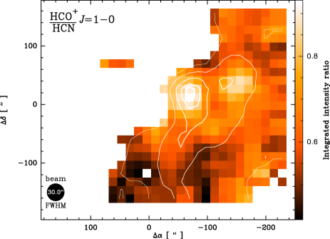
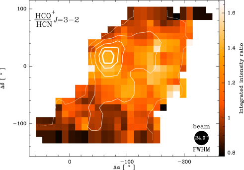
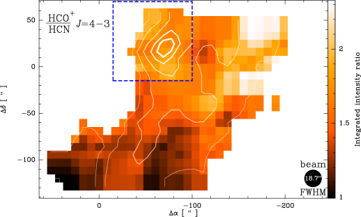
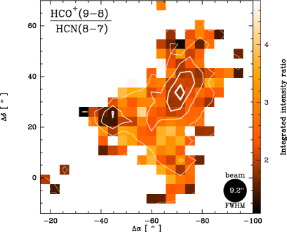
Figure 6: Maps of the HCO⁺/HCN ratio between the $J=1\to 0$ (top-left), $J=3\to 2$ (top-right) and $J=4\to 3$ (bottom-left) line integrated intensities in the region where the lines are brighter than 7% of their peak values. The $J=1\to 0$ ratio varies between about 0.4 and 0.9. The isolated ratios shown at $\Delta\delta\sim 70^{\prime\prime}$ correspond to significant emission of $\sim$30 ${\rm K}\,{\rm km}\,{\rm s}^{-1}$ in both HCN and HCO⁺ $J=1\to 0$ lines. The $J=3\to 2$ line ratio ranges from $\sim 0.8$ to $\sim 1.7$ while the $J=4\to 3$ line ratio varies between $\sim 1.0$ and $\sim 2.3$. The contour lines correspond to the HCO⁺ $J=1\to 0$, $J=3\to 2$ and $J=4\to 3$ maps in the respective line ratios, and are defined as in Fig. 2. The HCO⁺ $J=9\to 8$ to HCN $J=8\to 7$ line ratio is shown in the bottom-right panel, for the region where the lines are brighter than the 15% of their peak values. This ratio varies between about unity to $\sim$4.8. The contour lines correspond to the HCN $J=8\to 7$ maps and are the same as in Fig. 3. The area of the higher-$J$ HCN and HCO⁺ ratio map is depicted with a dashed frame in the bottom-left panel. The maps of the higher frequency lines were convolved to the larger beam of the lower frequency line before determining the respective ratios.

3.4 The HCO⁺/HCN line intensity ratios

The HCO⁺ $J=4\to 3$ map was convolved with the slightly larger beam size ($17.7^{\prime\prime}$) of the HCN $J=4\to 3$ line, in order to have the same number of pixels per map. The pixel size is $8.9^{\prime\prime}\times 8.9^{\prime\prime}$ which ensures Nyquist sampling of the spectra in both (R.A. and Dec.) directions. Likewise, the HCO⁺ $J=3\to 2$ map was convolved with the beam size ($23.6^{\prime\prime}$, and spatial resolution of $11.8^{\prime\prime}\times 11.8^{\prime\prime}$) of the HCN $J=3\to 2$ line before computing the ratio between the respective maps. The HCO⁺ $J=9\to 8$ was convolved to the larger beam of the HCN $J=8\to 7$ line to match its spatial resolution ($9.2^{\prime\prime}$). The same was done for the $J=1\to 0$ maps, but convolved to a $30^{\prime\prime}$ beam.

In order to reduce uncertainties and avoid misleading values in zones with relatively low S/N and no clear detection, we compute the HCO⁺/HCN $J=4\to 3$, $J=3\to 2$ and $J=1\to 0$ line intensity ratios only in the region where the integrated temperature of both lines (in both species) is brighter than 7% of their peak values. That is, between 5$\sigma$ and 8$\sigma$, where $\sigma$ is the rms of the HCN and HCO⁺ $J=4\to 3$ and $J=3\to 2$ maps, which ranges between 0.2 K and 0.3 K. In the case of the $J=1\to 0$ lines the rms is one order of magnitude lower. Due to the lower S/N of the HCN $J=8\to 7$ (the fainter line), we used a threshold of 15% for the higher-$J$ line ratio. This corresponds to about 6$\sigma$ in both HCN $J=8\to 7$ and HCO⁺ $J=9\to 8$, with rms values of 0.62 K and 1.24 K, respectively. Because the HCN and HCO⁺ maps were observed simultaneously with practically the same beam size, our results are not affected by relative pointing errors.

All the HCO⁺/HCN line intensity ratios are shown in Fig. 6. The HCO⁺/HCN $J=1\to 0$ line ratio is lower than unity in most of the region mapped. The fact that the higher-$J$ HCN/HCO⁺ intensity ratio becomes larger than unity may be due to infrared pumping of the HCN $J=1\to 0$ line through a vibrational transition at 14 $\mu$m wavelength. This mechanism can produce an enhanced HCN $J=1\to 0$ emission in conditions of sub-thermal excitation, as discussed in the next section.

The HCO⁺/HCN $J=3\to 2$ line intensity ratio ranges between $\sim 0.8$ and $\sim 1.7$, while the intensity of the HCO⁺ $J=4\to 3$ line is a factor $\sim 1-2$ brighter than that of the HCN line, as shown in Fig. 6. The line profiles of both lines match very well in all the positions, which indicates that the difference in intensities is not a consequence of different line widths.

With a higher spatial resolution ($9\aas@@fstack{\prime\prime}2$) the line intensity ratio HCO⁺($9\to 8$)/HCN($8\to 7$) shows the largest values (up to $\sim$4.8) of the four ratio maps. The ratio is lowest (between $\sim$1 and $\sim$2) at the region of the strongest HCN $J=8\to 7$ emission (as shown by the contours in the bottom-right panel of Fig. 6), which coincides with the M17-UC1 region (south-east peak) and the peak of the HCN $J=8\to 7$ line (north-west peak). The relatively bright HCN emission in these two regions can be explained by dense and warm gas, and by the presence of hot cores (or UC-H II regions) (e.g., Prasad et al. 1987; Caselli et al. 1993; Viti & Williams 1999; Rodgers & Charnley 2001).

Similar high HCO⁺/HCN $J=4\to 3$ line ratios have been observed in other Galactic star forming regions (e.g., W49A Peng et al. 2007), while HCO⁺/HCN $J=4\to 3$ line ratios lower than unity have been found from single dish observations of active galaxies like NGC 1068 (Pérez-Beaupuits et al. 2009) and in recent ALMA observations (García-Burillo et al. 2014; Viti et al. 2014, note that for the ALMA observations the authors quote the inverse HCN/HCO⁺ line ratio instead). According to models by Meijerink et al. (2007, their Fig. 14), however, HCO⁺/HCN $J=4\to 3$ line ratios lower than unity are signatures of a high density ($>10^{4}\leavevmode\nobreak\ \rm{cm^{-3}}$) PDR environment rather than an X-ray dominated region (XDR), as suggested by García-Burillo et al. (2014). But interpretations of the HCO⁺/HCN line ratios in extragalactic environments may not be as straight forward as believed in the past, since these species are now known to be strongly time-dependent in both dense gas (e.g. Bayet et al. 2008) and in XDRs (e.g. Meijerink et al. 2013), as pointed out by Viti et al. (2014). Hence, the HCO⁺/HCN line ratios observed in galaxies may reflect departures from chemical equilibrium rather than differences in the underlying excitation environment.

3.4.1 Infrared pumping of the dense molecular gas?

In environments with high enough UV/X-ray surface brightness to heat the dust to several hundred K, like in AGNs, bright starbursts or massive star-forming regions in the Galaxy and the circumnuclear disk (CND) around the massive black hole at the center of our Galaxy, strong HCN, HNC, and HCO⁺ emission in the sub-millimeter and millimeter range may also be explained by the infrared radiative pumping scenario (e.g. Aalto et al. 1995; Christopher et al. 2005; García-Burillo et al. 2006; Guélin et al. 2007; Aalto et al. 2007b, a), since hot dust produces strong mid-infrared continuum emission in the 10–30 $\mu$m wavelength range.

If the infrared pumping scenario is at work, absorption features must be detected in infrared spectra at 12.1 $\mu$m, 14.0 $\mu$m, and 21.7 $\mu$m, which are the wavelengths of the ground vibrational states of HCO⁺, HCN, and HNC, respectively, connected by the transitions $\nu_{2}=1$ of the lowest excited bending states. At the moment we do not have high resolution IR spectra to check if this is the case in all the mapped region of M17 SW. On the other hand, the HCN $J=4\to 3$, $\nu_{2}=1$ transition (356.256 GHz) was detected with a peak intensity of $\sim$50 mK towards the CND of the Milky Way (Mills et al. 2013), indicating radiative pumping of HCN at 14.0 $\mu$m. However, we did not detect this vibrationally excited HCN line, which lies close to our HCO⁺ spectra, at an rms level of $\sim$1 mK. Besides, the fact that the HCO⁺/HCN line ratio grows monotonically with $J$-level can be considered an argument against 14 $\mu$m pumping. Therefore, we think the HCN and HCO⁺ lines in M17 SW are unlikely to be affected by infrared pumping.

3.4.2 Other causes of high HCO⁺/HCN line ratios

Due to the smaller physical scales and the different metallicity, the time-dependency of the abundance of HCN compared to that of HCO⁺ should not be an issue in Galactic molecular clouds. However, the bulk HCO⁺ emission may still arise from gas that does not co-exist (in terms of ambient conditions or, equivalently, from a different layer within a clump) with the gas hosting the HCN, as previously suggested by Pérez-Beaupuits et al. (2009, their Apendix C.3).

Stronger HCO⁺ emission could also be the consequence of the higher ionization degree in X-ray dominated regions (XDRs), which leads to an enhanced HCO⁺ formation rate (e.g. Lepp & Dalgarno 1996; Meijerink & Spaans 2005). Using the XDR models by Meijerink & Spaans (2005) we estimate that in order to drive an XDR, an X-ray source (or a cluster of sources) with a (combined) impinging luminosity of at least $10^{32}\leavevmode\nobreak\ {\rm{erg}\leavevmode\nobreak\ {s^{-1}}}$ would be required to be within a few arcsecs ($<0.03$ pc in M17 SW) from the region of the HCO⁺ $J=4\to 3$ peak emission, considering that the X-ray flux decreases with the square of the distance from the source.

Based on the luminosities estimated from thermal plasma (546 sources) and power law fits (52 sources) of the photometrically selected Chandra/ACIS sources by Broos et al. (2007), we estimate that the combined X-ray luminosity (integrated between 0.5 keV and 50 keV, and projected on the sky at the position of the peak HCO⁺ emission) is about three orders of magnitude lower than needed to drive an XDR. This result rules out an XDR scenario to explain the relatively strong HCO⁺ emission. However, our estimates are based on an X-ray SED fit, extrapolated up to 50 keV with no actual observations above 10 keV (the upper band of Chandra/ACIS). Higher energy ($>$10 keV) photons could make a larger contribution to the X-ray flux, particularly from sources that have significant power-law tails. However, unless such X-ray sources would be located sufficiently close to (or within) the region with bright HCO⁺ emission, they probably could not increase the required X-ray flux by three orders of magnitude. In fact, no X-ray source was detected by Chandra/ACIS within a radius of $\sim$10^′′ ($\sim$0.09 pc) around the peak HCO⁺ emission. This either rules out the existence of any X-ray source in that region or implies that all X-ray photons with energy $<$10 keV are heavily absorbed by the large column density of the gas ($\sim$8$\times$10${}^{23}\leavevmode\nobreak\ \rm{cm^{-2}}$, Stutzki & Güsten 1990). Therefore, future observations sensitive to higher energy ($kT>10$ keV) photons that could escape the large column of gas, are required to unambiguously discard any heavily obscured X-ray source that may exist in the dense core of M17 SW.

Besides X-rays there are other possible mechanisms that can also lead to a relatively bright HCO⁺ emission. Indeed, if the intensity of emission from HCO⁺ is as strong as that from HCN (or stronger) it may be due to relatively high kinetic temperatures, strong UV radiation fields, and relatively lower densities of the gas from where the HCO⁺ emission emerges (e.g. Fuente et al. 1993; Chin et al. 1997; Brouillet et al. 2005; Christopher et al. 2005; Zhang et al. 2007; Meijerink et al. 2007).

Since HCN and HCO⁺ are expected to co-exist at similar depths in a cloud, the kinetic temperature of their surrounding gas must also be similar. But the critical density of the HCO⁺ lines is one order of magnitude lower than that of HCN (cf., Table 1), which makes HCO⁺ more easily excited (collisionally) in single-phase molecular gas. Because the HCO⁺/HCN line ratio reflects the effects of the combination of abundance and excitation temperature, the increasing ratio with $J$-line can be indicative of a lower excitation temperature in the higher-$J$ transitions of HCN. We explore this alternative through excitation models in Sect.4.

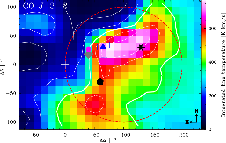
Figure 7: Velocity-integrated intensity map of ¹²CO $J=3\to 2$, convolved a $25^{\prime\prime}$ beam to match the resolution of the ¹²CO $J=11\to 10$ map. The contour levels are the 10%, 25%, 50% (thick line), 75% and 90% of the peak emission (770 ${\rm K}\,{\rm km}\,{\rm s}^{-1}$). The central position ($\Delta\alpha=0$, $\Delta\delta=0$) marked with a white cross, is the same as in Fig. 1. The ultracompact H II region M17-UC1 and four H₂O masers (Johnson et al. 1998) are marked by the filled circle and plus symbols, respectively. The positions of the peak intensities of HCN $J=8\to 7$ and ¹²CO $J=16\to 15$, as well as the offset positions at ($-60^{\prime\prime}$,$-30^{\prime\prime}$) and ($-130^{\prime\prime}$,$+30^{\prime\prime}$) analyzed in Sec. 4.4, are indicated with a triangle, a diamond, a pentagon and a star, respectively.

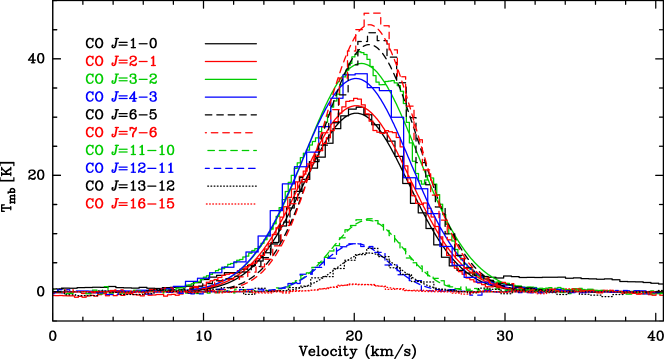
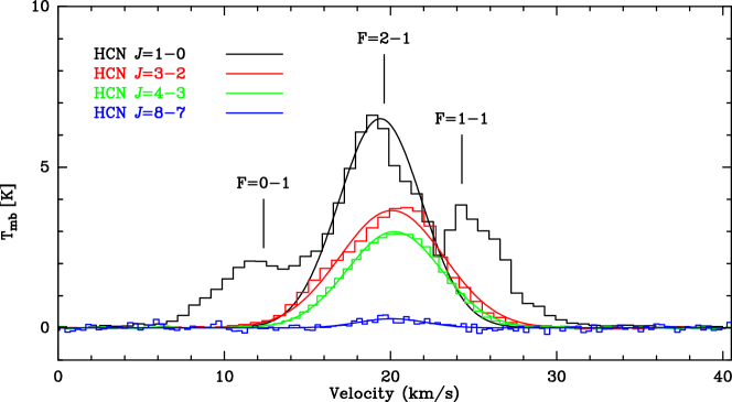
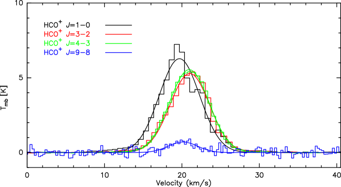
Figure 8: Average spectra of ¹²CO (top), HCN (middle - indicating the hyperfine structure lines of HCN $J=1\to 0$ ) and HCO⁺ (bottom), obtained from the $200^{\prime\prime}$-beam area (dashed circle in Fig. 7) toward M17SW, centered at offset position ($-100^{\prime\prime}$,$0^{\prime\prime}$). This correspond to a region of $\sim$1.92 pc in diameter at the distance of 1.98 kpc (Xu et al. 2011).

4 Analysis of the LSEDs

We first computed the average spectra of a 200 arcsec² region to mimic the results obtained when observing extragalactic sources with ALMA. These average spectra can be fit using a single Gaussian component, as shown in Fig. 8.

Then we analyze the spectra from the 25^′′ resolution maps at four selected positions in M17 SW. The profiles of the CO lines show a very rich structure due to the clumpiness of the source (several velocity components along the line of sight) and to optical depth effects (self-absorption) of the lower-$J$ transitions (cf., Fig. 10). While the lower- and mid-$J$ ¹²CO lines can be fit with up to five Gaussian components, the higher-$J$ ($J_{up}\geq 11$) can be fit with just one or two Gaussian components. In order to ensure we are comparing the line fluxes corresponding to the same velocity component, we chose the Gaussian component of the lower- and mid-$J$ lines that is the closest related to the central velocity and line width obtained for the single Gaussian used to fit the ¹²CO $J=16\to 15$ line.

The profiles of the HCN and HCO⁺ lines also show structures that could be associated with different overlapping cloudlets along the line of sight. However, contrarily to the ¹³CO lines, the H¹³CN and H¹³CO⁺ lines do not show the same structure as the main isotope lines. (cf., Figs. 11 and 12). With the exception of the $J=1\to 0$ transitions, the higher-$J$ ¹³C bearing lines seem to be made of a single component that can be fit with one Gaussian. This is indicative of self-absorption (or optical depth effects) in the ¹²C lines. Therefore, instead of using several Gaussian components in the HCN and HCO⁺ lines, we fit a single component trying to reproduce the missing flux by using just the apparently less self-absorbed emission in the line wings and masking the line centers for the Gaussian fit. The fluxes obtained in this way are significantly larger (between 13% and 95%, depending on the line and the offset position) for the HCN lines, compared to the flux obtained by using two or more Gaussian components. The HCO⁺ lines show a lower degree of self-absorption.

After obtaining the velocity-integrated intensities from the Gaussian fit, we convert the intensities to fluxes in units of erg s^-1 cm^-2 sr^-1 as $F_{\nu_{0}}^{\prime}=10^{5}k\left(\frac{\nu_{0}}{c}\right)^{3}\int T_{mb}dv$, where $k$ is the Boltzmann’s constant, $\nu_{0}$ is the rest frequency of the transition, $c$ is the speed of light and the factor $10^{5}$ is to convert from ${\rm km\,s}^{-1}$ to cm s^-1. This flux is then converted to units of W m² by $F_{\nu_{0}}=10^{-7}F_{\nu_{0}}^{\prime}\Omega_{25^{\prime\prime}}10^{4}$ with $\Omega_{25^{\prime\prime}}$ the 25^′′ beam solid angle (resolution) used in our maps, the factor $10^{4}$ is to convert from cm² to m², and the factor $10^{-7}$ to convert from erg s^-1 to Watts.

We model the observed fluxes using the modified RADEX code (van der Tak et al. 2007) that uses a background radiation field, as done by Poelman & Spaans (2005) and Pérez-Beaupuits et al. (2009), and considering a dust temperature of 50 K found by Meixner et al. (1992) toward M17 SW.

We chose this modified background radiation field because interaction with far- and mid-infrared radiation (mainly from dust emission in circumstellar material or in star- forming regions) can be important for molecules with widely spaced rotational energy levels (e.g., the lighter hydrides OH, H₂O, H₃O⁺ and NH₂), and particularly for the higher-$J$ levels of heavy molecular rotors such as CO, CS, HCN, HCO⁺ and H₂CO, that are observable with Herschel and SOFIA in the far- and mid-infrared regime. However, the actual effect of the dust IR emission on the redistribution among rotational levels of a molecule depends on the local ambient conditions of the emitting gas. That is because at high densities (or temperatures) collisions are expected to dominate the excitation of the mid- and high-$J$ levels of molecules, such as CO, while at lower densities (or temperatures) radiative excitation, as well as spontaneous decay from higher-$J$ levels, are expected to be the dominant component driving the redistribution of the level populations. Since we do not know a priori what the ambient conditions are at the selected positions in M17 SW, we include the modified background radiation field for completeness.

The RADEX code computes the local escape probability assuming a uniform temperature and density of the collision partners. For the case of M17 SW the escape probability can be computed using two independent methods implemented in RADEX: the large velocity gradient (LVG) formalism and assuming an homogeneous sphere geometry. We tested both methods against each other with a test fit of the LSEDs using low enough densities and column densities to ensure convergence. The results obtained with both methods were not significantly different for the CO LSEDs; the rms (or $\chi^{2}$) values obtained from the observed fluxes and those predicted by the two formalisms differ by just $\sim$2% between the methods, with the largest differences pertaining for $J_{up}>10$ CO lines. For the HCN lines, however, the LVG method gives about 34% higher intensities, while for the HCO⁺ lines the LVG method gives between 15% and 20% higher intensities. In order to obtain similar HCN and HCO⁺ line intensities as with the LVG method the uniform sphere formalism requires larger column densities and slightly larger filling factors. When using relatively large densities ($>$4$\times$10${}^{5}\leavevmode\nobreak\ \rm{cm^{-3}}$) and column densities ($>$2$\times$10${}^{15}\leavevmode\nobreak\ \rm{cm^{-2}}$) for HCN the LVG method did not converge. Since these parameters ranges turned out to be relevant for a good fit of the LSEDs, we used the uniform sphere geometry method in our models. The physical conditions were modeled using the collisional data available in the LAMDA database (Schöier et al. 2005). The collisional rate coefficients for ¹²CO are adopted from Yang et al. (2010).

4.1 The Spectral Line Energy Distribution

We had to fit the full LSEDs of the ¹²CO, HCN, and HCO⁺ lines by assuming a cold and a warm component. A single component does not fit all the fluxes and three components require more free parameters than the available number of observations (particularly for the HCN and HCO⁺ lines). The model we use is described by:

$$F_{tot}(\nu)=\Phi_{cold}F_{cold}+\Phi_{warm}F_{warm}$$ (1)

where $\Phi_{i}$ are the beam area filling factors and $F_{i}$ are the estimated fluxes for each component in units of ${\rm{W}\leavevmode\nobreak\ {{m^{-2}}}}$. The estimated fluxes of the main isotopologues (i.e., ¹²C-bearing molecules) are a function of four parameters per component: the beam area filling factor $\Phi$, the density of the collision partner $n(\rm H_{2})$ ($\rm{cm^{-3}}$), the kinetic temperature of the gas $T_{k}$ (K), and the column density per line width $N/\Delta V$ (${\rm cm}^{-2}\,{\rm km}^{-1}\,{\rm s}$) of the molecule in study. We used the average FWHM obtained from the Gaussian fit of the $J_{up}>2$ lines for the line widths $\Delta V$ of a given species (the $J_{up}\leq 2$ transitions were not considered because their emission was collected with a beam size larger than 25^′′).

The two component fit of the LSED requires eight free parameters. We use the simplex method (e.g., Nelder & Mead 1965; Kolda et al. 2003) to minimize the error between the observed and estimated fluxes, using sensible initial values and constraints of the input parameters as described below. The uncertainty in the parameters is obtained by allowing solutions of the LSED fit in a $3\sigma$ range around the estimated fluxes, where $\sigma$ includes the standard deviation of the fluxes obtained from the Gaussian fit and 20% of calibration uncertainties.

We also included all the available ¹³CO fluxes to constrain mainly the column density. We use the same excitation conditions (density and temperature) as for ¹²CO. The same was done for the H¹³CN and H¹³CO⁺ lines. In order to reduce the number of free parameters, we use the same filling factors for the ¹³C as for the ¹²C bearing lines in the cold and warm component. This is a reasonable assumption since the ¹³C lines, although usually fainter and less extended when shown in linear scale, appear as extended as the ¹²C lines when shown in logarithmic scale.

Because for HCN and HCO⁺ we have fewer transitions than for CO, we first fit the CO LSED and then used the same density and temperature found for the cold and warm components from CO for fitting the HCN and HCO⁺ LSEDs.

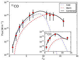
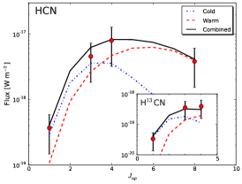
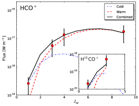
Figure 9: Two component fit of the line spectral energy distribution of the CO, HCN, and HCO⁺ species, for the average spectra toward M17 SW. The fit of the ¹³C bearing isotopologues are shown in the insets. The cold and warm components are shown in dotted and dashed lines, respectively. The error bars correspond to the 3$\sigma$ range used to estimate the standard deviation of the excitation parameters, where $\sigma$ is the flux uncertainties obtained from the Gaussian fit.

Table 2: Gaussian fit parameters for the average spectra.

Transition	$\int T_{mb}dV$	$T_{mb}^{peak}$	$V_{0}$	$\Delta V$ (FWHM)
	[${\rm K}\,{\rm km}\,{\rm s}^{-1}$]	[K]	[${\rm km\,s}^{-1}$]	[${\rm km\,s}^{-1}$]
12CO
$J=1\to 0$	264.0$\pm$ 5.2	30.66$\pm$0.95	19.89$\pm$ 0.08	8.09$\pm$ 0.19
$J=2\to 1$	282.9$\pm$ 1.0	31.95$\pm$0.18	19.88$\pm$ 0.02	8.32$\pm$ 0.04
$J=3\to 2$	360.4$\pm$ 0.0	39.20$\pm$0.01	20.21$\pm$ 0.00	8.64$\pm$ 0.00
$J=4\to 3$	328.0$\pm$ 0.1	36.62$\pm$0.01	19.86$\pm$ 0.00	8.41$\pm$ 0.00
$J=6\to 5$	342.7$\pm$ 0.0	42.43$\pm$0.00	20.73$\pm$ 0.00	7.59$\pm$ 0.00
$J=7\to 6$	354.3$\pm$ 1.0	45.84$\pm$0.20	20.75$\pm$ 0.01	7.26$\pm$ 0.02
$J=11\to 10$	72.0$\pm$ 0.5	12.30$\pm$0.15	20.63$\pm$ 0.02	5.50$\pm$ 0.05
$J=12\to 11$	44.9$\pm$ 0.7	8.28$\pm$0.22	19.87$\pm$ 0.04	5.10$\pm$ 0.10
$J=13\to 12$	34.7$\pm$ 1.2	6.69$\pm$0.38	20.65$\pm$ 0.08	4.87$\pm$ 0.21
$J=16\to 15$	5.9$\pm$ 0.4	1.31$\pm$0.16	20.10$\pm$ 0.16	4.28$\pm$ 0.41
13CO
$J=1\to 0$	63.0$\pm$ 0.7	10.88$\pm$0.19	19.74$\pm$ 0.03	5.44$\pm$ 0.07
$J=2\to 1$	169.0$\pm$ 0.0	26.91$\pm$0.01	19.96$\pm$ 0.00	5.90$\pm$ 0.00
$J=3\to 2$	157.6$\pm$ 0.4	24.35$\pm$0.09	20.09$\pm$ 0.01	6.08$\pm$ 0.02
$J=6\to 5$	124.6$\pm$ 0.0	21.67$\pm$0.00	20.57$\pm$ 0.00	5.40$\pm$ 0.00
$J=13\to 12$	1.9$\pm$ 0.5	0.28$\pm$0.13	20.39$\pm$ 0.91	6.62$\pm$ 2.55
HCN
$J=1\to 0$	40.1$\pm$ 1.8	6.51$\pm$0.29	19.15$\pm$ 0.20	5.80$\pm$ 0.00
$J=3\to 2$	28.3$\pm$ 0.0	3.65$\pm$0.00	19.84$\pm$ 0.00	7.29$\pm$ 0.00
$J=4\to 3$	20.9$\pm$ 0.0	3.00$\pm$0.01	19.98$\pm$ 0.01	6.57$\pm$ 0.02
$J=8\to 7$	1.4$\pm$ 0.1	0.29$\pm$0.04	19.84$\pm$ 0.25	4.77$\pm$ 0.53
H13CN
$J=1\to 0$	5.7$\pm$ 0.1	0.60$\pm$0.02	19.61$\pm$ 0.09	9.01$\pm$ 0.23
$J=3\to 2$	2.1$\pm$ 0.0	0.39$\pm$0.03	19.44$\pm$ 0.11	5.06$\pm$ 0.26
$J=4\to 3$	1.0$\pm$ 0.0	0.23$\pm$0.01	19.56$\pm$ 0.06	4.47$\pm$ 0.14
HCO+
$J=1\to 0$	40.7$\pm$ 0.1	6.28$\pm$0.02	19.43$\pm$ 0.00	6.09$\pm$ 0.01
$J=3\to 2$	33.2$\pm$ 0.0	5.29$\pm$0.02	20.76$\pm$ 0.00	5.91$\pm$ 0.02
$J=4\to 3$	34.9$\pm$ 0.0	5.54$\pm$0.01	20.69$\pm$ 0.00	5.92$\pm$ 0.01
$J=9\to 8$	3.3$\pm$ 0.4	0.71$\pm$0.16	19.88$\pm$ 0.25	4.40$\pm$ 0.79
H13CO+
$J=1\to 0$	3.7$\pm$ 0.0	0.80$\pm$0.02	19.51$\pm$ 0.03	4.37$\pm$ 0.07
$J=3\to 2$	3.4$\pm$ 0.1	0.75$\pm$0.03	20.19$\pm$ 0.06	4.32$\pm$ 0.15

Table 3: LSED fit parameters for the average spectra.

Parameter	CO	HCN	HCO+
$\Phi_{cold}(^{12}{\rm C})$	1.00 $\pm$ 0.13	0.60 $\pm$ 0.07	0.60 $\pm$ 0.07
$n_{cold}(\rm H_{2})$ [cm-3]	4.80 $\pm$ 0.25	4.80 $\pm$ 0.49	4.80 $\pm$ 0.54
$T_{cold}$ [K]	42.00 $\pm$ 3.71	42.00 $\pm$ 3.91	42.00 $\pm$ 4.38
$N_{cold}$ [cm-2]	19.50 $\pm$ 0.48	15.40 $\pm$ 1.19	14.20 $\pm$ 0.88
$\Phi_{warm}(^{12}{\rm C})$	0.10 $\pm$ 0.01	0.10 $\pm$ 0.01	0.10 $\pm$ 0.01
$n_{warm}(\rm H_{2})$ [cm-3]	6.00 $\pm$ 0.60	6.00 $\pm$ 0.77	6.00 $\pm$ 0.48
$T_{warm}$ [K]	135.00 $\pm$ 8.46	135.00 $\pm$ 12.09	135.00 $\pm$ 15.51
$N_{warm}$ [cm-2]	18.10 $\pm$ 0.36	14.70 $\pm$ 0.94	14.40 $\pm$ 0.50
$\Phi_{cold}(^{13}{\rm C})$	1.00 $\pm$ 0.12	0.60 $\pm$ 0.06	0.60 $\pm$ 0.05
$\Phi_{warm}(^{13}{\rm C})$	0.10 $\pm$ 0.00	0.10 $\pm$ 0.01	0.10 $\pm$ 0.01
$\Delta V(^{12}{\rm C})$ [km s${}^{-}1$]	8.00	6.00	6.00
$\Delta V(^{13}{\rm C})$ [km s${}^{-}1$]	6.00	6.00	4.00

4.2 Constraints on the model parameters

Two of the most critical parameters of the models are the column densities and the beam area filling factors. The filling factors were discussed above, while the column densities depend on the observed fluxes and the excitation conditions (temperature and density) of the models.

Another important parameter of the models is the carbon-12 to carbon-13 isotope ratio, which couples the column densities of the ¹²C and ¹³C lines since we assume $N({\rm{}^{13}CO})=N({\rm{}^{12}CO})/\mathcal{R}_{12/13}$, with $\mathcal{R}_{12/13}$=[¹²C]/[¹³C]. The isotope ratio $\mathcal{R}_{12/13}$ is known to vary from source to source in the Milky Way, depending on the distance to the Galactic center (e.g. Henkel et al. 1982, 1985; Langer & Penzias 1990; Milam et al. 2005). At a distance of 1.98 kpc (Xu et al. 2011), M17 SW is expected to have a CO isotope ratio of $\mathcal{R}_{12/13}=51.6\pm 7.9$, according to Eq. (3) by Milam et al. (2005). In our models we use $\mathcal{R}_{12/13}=50$. For HCN and HCO⁺ the same isotope ratio as for CO can be considered. However, there is theoretical and observational evidence that the actual HCN isotope ratio is closer to that obtained from observations of H₂CO, which provides an upper limit to $\mathcal{R}_{12/13}$ while CO provides a lower limit, and isotope ratios derived from HCO⁺ lead to intermediate values (e.g. Langer et al. 1984; Henkel et al. 1985; Milam et al. 2005). Thus, from Eqs. (5) and (4) by Milam et al. (2005), the isotope ratios for HCO⁺ and HCN in M17 SW should be $\sim$56 and $\sim$63, respectively. Using these higher $\mathcal{R}_{12/13}$ values, however, we could not fit the HCN and HCO⁺ LSEDs simultaneously with the H¹³CN and H¹³CO⁺ lines. We were able to fit the HCN and HCO⁺ LSEDs using the same isotope ratio of 50 as for the CO lines, although smaller $\mathcal{R}_{12/13}$ of 30 and even 20, would lead to a better fit of the rare HCN and HCO⁺ isotopologues. This would be in agreement with the more recent results found by Röllig & Ossenkopf (2013) for HCO⁺, but not for the HCN isotope ratio. The discrepancy we found for HCN is likely due to optically thick lines which are also heavily affected by self-absorption, as mentioned in Sect. 4.

4.3 Excitation of the Average Emission in M17 SW

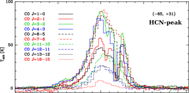
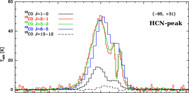
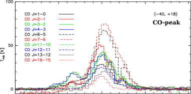
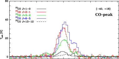
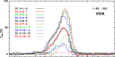
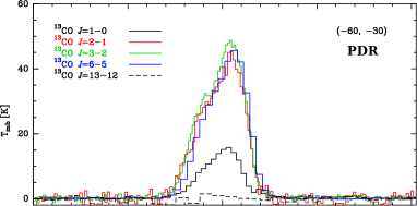
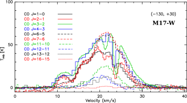
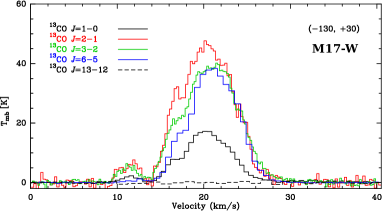
Figure 10: Spectra of all ¹²CO (left panel) and ¹³CO (right panel) lines observed at the four selected offset (within $\pm$3^′′) positions shown in Fig. 7. All the spectra, except the $J=1\to 0$ and $J=2\to 1$ have been convolved with a 25^′′ beam, corresponding to the ¹²CO $J=11\to 12$ map.

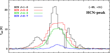
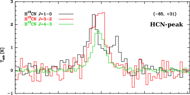
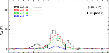
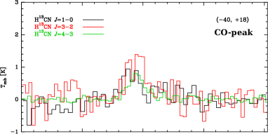
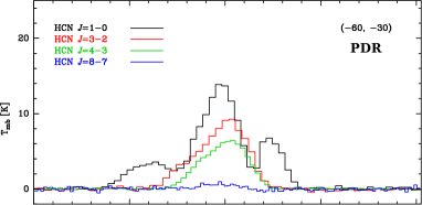
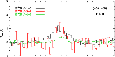
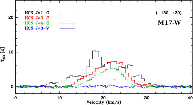
Figure 11: Spectra of all HCN (left panel) and H¹³CN (right panel) lines observed at the four selected offset (within $\pm$3^′′) positions shown in Fig. 7. All the spectra, except the $J=1\to 0$ and $J=2\to 1$ have been convolved with a 25^′′ beam, corresponding to the ¹²CO $J=11\to 12$ map.

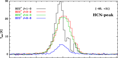
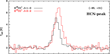
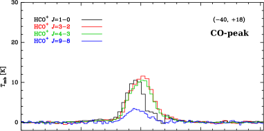
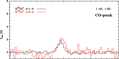
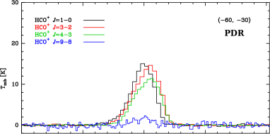
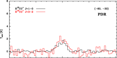
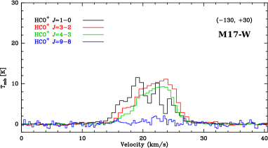
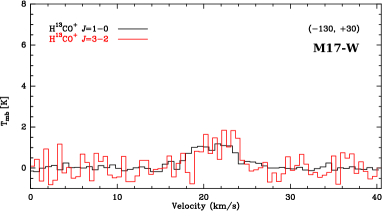
Figure 12: Spectra of all HCO⁺ (left panel) and H¹³CO⁺ (right panel) lines observed at the four selected offset (within $\pm$3^′′) positions shown in Fig. 7. All the spectra, except the $J=1\to 0$ and $J=2\to 1$ have been convolved with a 25^′′ beam, corresponding to the ¹²CO $J=11\to 12$ map.

We computed the average spectrum in a region associated with a 200^′′ beam size, centered at offset position ($-100^{\prime\prime}$,$0^{\prime\prime}$), in order to estimate the excitation derived from ALMA observations of nearby Galaxies. In M17 SW the $200^{\prime\prime}$ beam covers a spatial scale of $\sim$2 pc. This correspond to the spatial scale that would be resolved by ALMA with the finest achievable angular resolution ($0.03^{\prime\prime}$ with the capabilities available in Cycle 3) of the bands 6 (230 GHz) and 10 (870 GHz) towards a galaxy like NGC 1068 at a distance of $\sim$14.4 Mpc. Coarser angular resolution would be sufficient to resolve the same spatial scale in closer galaxies like NGC 253 (at $\sim$3.5 Mpc).

Figure 7 shows the ¹²CO $J=3\to 2$ map convolved with a 25^′′ beam, and the dashed circle depicts the area where the average emission in all the maps was estimated from. The average spectra of the ¹²CO, HCN and HCO⁺ lines are shown in Fig. 8. We computed the intensities integrating the spectra over the 5–35 ${\rm km\,s}^{-1}$ velocity range. We also fit one Gaussian component to estimate the (FWHM) line width. The velocity-integrated intensities and the total intensity obtained from the Gaussian fit are similar within a few percent.

The best two components model fit of Eq. 1 is shown in Fig. 9 for ¹²CO, HCN and HCO⁺. The LSED fit of the isotopologues, ¹³CO, H¹³CN and H¹³CO⁺, is shown in the insets. The error bars correspond to the $3\sigma$ range around the fluxes used to estimate the standard deviation of the parameters, where $\sigma$ is the uncertainty of the estimated fluxes obtained from the Gaussian fit. Even though the fluxes of the HCN fine structure lines are not considered in the Gaussian fit, the flux estimated for the HCN $J=1\to 0$ line is similar than predicted by the model (Fig. 9, middle panel).

The parameters of the LSED models are summarized in Table $a$. Since the CO emission is more extended than the HCN and HCO⁺, the beam area filling factors of both CO components need to be larger as well. The same excitation conditions (density and temperature) as found for CO, were sufficient to reproduce the HCN and HCO⁺ fluxes, considering the same filling factors for these two species but with 37% and 84% lower column densities for the cold and warm component of HCO⁺, respectively. At first look, this might be counter-intuitive with the fact that the emission from the higher-$J$ ($J_{up}\geqslant 3$) transitions of HCO⁺ are brighter and seem to be more extended than those of HCN (cf., Figs. 2 and 3). But this can be explained because HCO⁺ is easier to excite than HCN, given their different critical densities (see Table 1), and the larger optical depths of the HCN lines.

The densities and temperatures found for the cold component of CO are comparable with those found in starburst galaxies like, e.g. NGC 253 (Rosenberg et al. 2014, their Tables 2–4), but the warm component requires excitation conditions with at least one order of magnitude higher density and column density. Similar discrepancies are found when comparing with the excitation conditions estimated for Seyfert galaxies like NGC 1068 (Spinoglio et al. 2012, their Table 3). These differences may be due to an underestimated beam dilution effect in the extragalactic observations, as well as the fact that in their larger beams they collect emission emerging from a variety of molecular clouds with different sources of heating. Another factor affecting the determination of the excitation conditions in extragalactic observations is the dust extinction that seems to affect the high-$J$ CO lines at the large ($>$10${}^{24}\leavevmode\nobreak\ \rm{cm^{-2}}$) column densities observed towards their centers (e.g. Pineda et al. 2010; Etxaluze et al. 2013), which was not taken into account in the extragalactic studies.

We do not correct the higher-$J$ CO lines for dust extinction either since the dust extinction in M17 SW is expected to be less significant than towards circumnuclear regions, given that the total column densities estimated towards M17 SW are between one and two orders of magnitude smaller than towards our Galactic Center (e.g., Stutzki & Güsten 1990; Meixner et al. 1992) and the centers of other galaxies.

4.4 Excitation at key positions in M17 SW

Using the 25^′′ resolution maps we estimated the fluxes from the Gaussian fit of the line wings, as described in the third paragraph of Sect. 4. Then we fit the LSED of the three molecular species at four particular locations toward M17 SW to study the variation in excitation conditions.

We chose the peak of the HCN $J=8\to 9$ emission at about the offset position ($-65^{\prime\prime}$,$+31^{\prime\prime}$) which is expected to be dominated by dense gas, the peak of the ¹²CO $J=16\to 15$ emission at about ($-40^{\prime\prime}$,$+18^{\prime\prime}$), close to the UC H II region, the emission at about ($-60^{\prime\prime}$,$-30^{\prime\prime}$), deeper into the PDR with an expected fair mixture of excitation conditions, and the emission at about ($-130^{\prime\prime}$,$+30^{\prime\prime}$) west from the northern concentration of H₂O masers, corresponding to the shoulder or secondary peak of the HCN and HCO⁺ strip lines of Fig. 5. We refer to these positions as: HCN-peak, CO-peak, PDR, and M17-W, respectively, and indicated in Fig. 7.

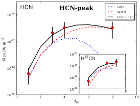
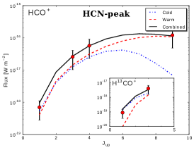
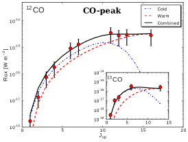
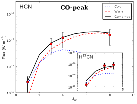
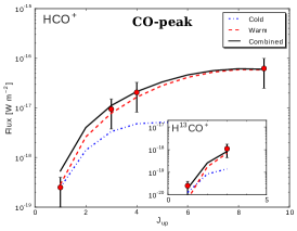
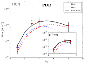
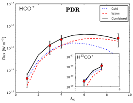
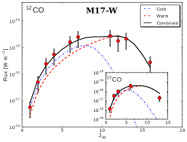
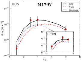
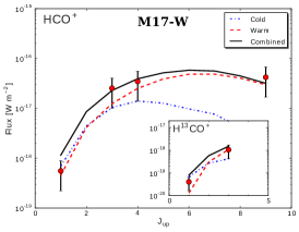
Figure 13: Two component fit of the line spectral energy distribution of the (from left to right) CO, HCN, and HCO⁺ species, for the (from top to bottom) spectra at offset position ($-65^{\prime\prime}$,$+31^{\prime\prime}$) toward the peak of the HCN $J=8\to 7$ intensity, ($-40^{\prime\prime}$,$+18^{\prime\prime}$) toward the peak of the ¹²CO $J=16\to 15$ intensity, ($-60^{\prime\prime}$,$-30^{\prime\prime}$) toward the PDR, and ($-130^{\prime\prime}$,$+30^{\prime\prime}$) toward the molecular gas in M17 SW. The fit of the ¹³C bearing isotopologues is shown in the insets. The cold and warm components are shown in dotted and dashed lines, respectively. The error bars are as in Fig. 9

The spectra of all the observed lines at these positions are shown in Figs. 10-12. The fluxes obtained from the CO, HCN and HCO⁺ spectra at the M17-W position have the largest uncertainties because the line profiles show the highest level of sub-structures and self-absorption features. The H¹³CN lines at this position have very low S/N, so we consider them as upper limits. The best fit models for the LSED at these positions are shown in Figs. 13, and the model parameters are summarized in Tables $a$, $a$, $a$ and $a$.

The ¹²CO LSED at the HCN-peak shows an increasing trend in flux with $J$, with an apparent turn over at the $J=14\to 13$ transition (which we do not have). The ¹²CO LSED of the CO-peak emission seems flat at the high-$J$ transitions, and the ¹²CO LSED at the PDR position, shows a decreasing trend in flux from the $J=11\to 10$ transition. On the other hand, the LSED of the M17-W position show a flat distribution of fluxes between the $J=7\to 6$ and $J=13\to 12$ transitions, and a sharp (one order of magnitude) decrease at the $J=16\to 15$. Observations of the $J=9\to 8$ transition with APEX would be needed to confirm the flat distribution of fluxes at the mid- and high-$J$ transitions of ¹²CO at the M17-W position. These different LSED shapes, specially at the high-$J$ CO lines obtained with SOFIA/GREAT, are indicative of the distinctive excitation conditions dominating mainly the warm component of the two-phase model.

Table 4: LSED fit parameters for the spectra toward the HCN-peak position ($-65^{\prime\prime}$,$+31^{\prime\prime}$).

Parameter	CO	HCN	HCO+
$\Phi_{cold}(^{12}{\rm C})$	1.00 $\pm$ 0.09	0.40 $\pm$ 0.05	0.40 $\pm$ 0.05
$n_{cold}(\rm H_{2})$ [cm-3]	4.50 $\pm$ 0.47	4.50 $\pm$ 0.47	4.50 $\pm$ 0.46
$T_{cold}$ [K]	40.00 $\pm$ 3.78	40.00 $\pm$ 5.37	40.00 $\pm$ 4.83
$N_{cold}$ [cm-2]	18.90 $\pm$ 1.12	16.60 $\pm$ 1.06	16.40 $\pm$ 1.08
$\Phi_{warm}(^{12}{\rm C})$	0.35 $\pm$ 0.04	0.15 $\pm$ 0.01	0.15 $\pm$ 0.02
$n_{warm}(\rm H_{2})$ [cm-3]	6.00 $\pm$ 0.73	6.00 $\pm$ 0.52	6.00 $\pm$ 0.48
$T_{warm}$ [K]	130.00 $\pm$ 11.59	130.00 $\pm$ 15.33	130.00 $\pm$ 14.03
$N_{warm}$ [cm-2]	18.40 $\pm$ 0.37	15.40 $\pm$ 0.54	15.20 $\pm$ 0.81
$\Phi_{cold}(^{13}{\rm C})$	1.00 $\pm$ 0.11	0.40 $\pm$ 0.05	0.40 $\pm$ 0.03
$\Phi_{warm}(^{13}{\rm C})$	0.35 $\pm$ 0.04	0.15 $\pm$ 0.02	0.15 $\pm$ 0.01
$\Delta V(^{12}{\rm C})$ [km s${}^{-}1$]	4.60	7.50	6.00
$\Delta V(^{13}{\rm C})$ [km s${}^{-}1$]	3.50	3.90	3.70

Table 5: LSED fit parameters for the spectra toward the CO-peak position ($-40^{\prime\prime}$,$+18^{\prime\prime}$).

Parameter	CO	HCN	HCO+
$\Phi_{cold}(^{12}{\rm C})$	0.50 $\pm$ 0.05	0.40 $\pm$ 0.05	0.40 $\pm$ 0.04
$n_{cold}(\rm H_{2})$ [cm-3]	4.80 $\pm$ 0.61	4.80 $\pm$ 0.46	4.80 $\pm$ 0.58
$T_{cold}$ [K]	90.00 $\pm$ 12.59	90.00 $\pm$ 8.21	90.00 $\pm$ 10.18
$N_{cold}$ [cm-2]	18.80 $\pm$ 0.35	15.30 $\pm$ 0.95	14.40 $\pm$ 1.33
$\Phi_{warm}(^{12}{\rm C})$	0.10 $\pm$ 0.01	0.10 $\pm$ 0.01	0.10 $\pm$ 0.01
$n_{warm}(\rm H_{2})$ [cm-3]	5.70 $\pm$ 0.35	5.70 $\pm$ 0.62	5.70 $\pm$ 0.50
$T_{warm}$ [K]	240.00 $\pm$ 29.77	240.00 $\pm$ 26.55	240.00 $\pm$ 26.54
$N_{warm}$ [cm-2]	18.50 $\pm$ 1.23	15.30 $\pm$ 1.10	15.10 $\pm$ 0.87
$\Phi_{cold}(^{13}{\rm C})$	0.50 $\pm$ 0.06	0.40 $\pm$ 0.04	0.40 $\pm$ 0.04
$\Phi_{warm}(^{13}{\rm C})$	0.10 $\pm$ 0.01	0.10 $\pm$ 0.01	0.10 $\pm$ 0.01
$\Delta V(^{12}{\rm C})$ [km s${}^{-}1$]	4.60	4.60	4.30
$\Delta V(^{13}{\rm C})$ [km s${}^{-}1$]	3.90	3.60	3.20

Table 6: LSED fit parameters for the spectra toward the southern PDR position ($-60^{\prime\prime}$,$-30^{\prime\prime}$).

Parameter	CO	HCN	HCO+
$\Phi_{cold}(^{12}{\rm C})$	0.90 $\pm$ 0.07	0.35 $\pm$ 0.04	0.35 $\pm$ 0.04
$n_{cold}(\rm H_{2})$ [cm-3]	5.30 $\pm$ 0.36	5.30 $\pm$ 0.49	5.30 $\pm$ 0.62
$T_{cold}$ [K]	60.00 $\pm$ 5.32	60.00 $\pm$ 6.82	60.00 $\pm$ 7.09
$N_{cold}$ [cm-2]	18.95 $\pm$ 0.47	15.40 $\pm$ 0.85	14.80 $\pm$ 1.13
$\Phi_{warm}(^{12}{\rm C})$	0.20 $\pm$ 0.01	0.15 $\pm$ 0.02	0.15 $\pm$ 0.02
$n_{warm}(\rm H_{2})$ [cm-3]	5.80 $\pm$ 0.37	5.80 $\pm$ 0.65	5.80 $\pm$ 0.56
$T_{warm}$ [K]	110.00 $\pm$ 11.56	110.00 $\pm$ 12.33	110.00 $\pm$ 13.42
$N_{warm}$ [cm-2]	18.60 $\pm$ 0.31	15.10 $\pm$ 1.10	14.70 $\pm$ 1.11
$\Phi_{cold}(^{13}{\rm C})$	0.90 $\pm$ 0.09	0.35 $\pm$ 0.04	0.35 $\pm$ 0.04
$\Phi_{warm}(^{13}{\rm C})$	0.20 $\pm$ 0.02	0.15 $\pm$ 0.02	0.15 $\pm$ 0.02
$\Delta V(^{12}{\rm C})$ [km s${}^{-}1$]	4.30	5.00	4.50
$\Delta V(^{13}{\rm C})$ [km s${}^{-}1$]	4.30	3.80	3.90

Table 7: LSED fit parameters for the spectra toward the M17-W position ($-130^{\prime\prime}$,$+30^{\prime\prime}$).

Parameter	CO	HCN	HCO+
$\Phi_{cold}(^{12}{\rm C})$	1.00 $\pm$ 0.00	0.80 $\pm$ 0.06	0.80 $\pm$ 0.09
$n_{cold}(\rm H_{2})$ [cm-3]	4.10 $\pm$ 0.00	4.10 $\pm$ 0.35	4.10 $\pm$ 0.49
$T_{cold}$ [K]	60.00 $\pm$ 0.00	60.00 $\pm$ 5.17	60.00 $\pm$ 7.12
$N_{cold}$ [cm-2]	19.00 $\pm$ 0.00	16.20 $\pm$ 0.53	15.40 $\pm$ 1.01
$\Phi_{warm}(^{12}{\rm C})$	0.40 $\pm$ 0.00	0.20 $\pm$ 0.02	0.20 $\pm$ 0.02
$n_{warm}(\rm H_{2})$ [cm-3]	5.80 $\pm$ 0.00	5.80 $\pm$ 0.39	5.80 $\pm$ 0.54
$T_{warm}$ [K]	80.00 $\pm$ 0.00	80.00 $\pm$ 8.61	80.00 $\pm$ 8.79
$N_{warm}$ [cm-2]	18.90 $\pm$ 0.00	15.10 $\pm$ 1.21	15.00 $\pm$ 0.56
$\Phi_{cold}(^{13}{\rm C})$	1.00 $\pm$ 0.00	0.80 $\pm$ 0.08	0.80 $\pm$ 0.09
$\Phi_{warm}(^{13}{\rm C})$	0.40 $\pm$ 0.00	0.20 $\pm$ 0.02	0.20 $\pm$ 0.02
$\Delta V(^{12}{\rm C})$ [km s${}^{-}1$]	6.90	6.10	7.10
$\Delta V(^{13}{\rm C})$ [km s${}^{-}1$]	5.50	6.10	4.40

The highest gas temperature of all selected positions was that of the warm component of the CO-peak, $\sim$240 K, which is in agreement with temperatures previously estimated toward the PDR interface from high- and mid-$J$ ¹²CO lines (e.g. Harris et al. 1987; Stutzki et al. 1988). Although the previous studies used larger beam sizes, probably collecting emission from colder gas, their estimates lead to a range of likely temperatures between 100 K and 500 K, and densities of few times $10^{4}\leavevmode\nobreak\ \rm{cm^{-3}}$. Instead the warm component of our two-phase models require between one and two orders of magnitude higher densities. This discrepancy in densities is explained because the previous estimates were based on line ratios of the ¹²CO $J=7\to 6$ and $J=14\to 13$ transitions, and line ratios of only two transitions are subject to the know dichotomy between density and temperature of the gas. Our estimates, instead, are constrained in great degree by the mid- and high-$J$ ¹³CO, H¹³CN, and H¹³CO⁺ isotopologue lines, which require high ($>10^{5}\leavevmode\nobreak\ \rm{cm^{-3}}$) densities to reproduce the observations. Lower densities ($<10^{4}\leavevmode\nobreak\ \rm{cm^{-3}}$) and higher temperatures ($>250\leavevmode\nobreak\ K$) produce low excitation temperatures of the ¹³C bearing molecules and, therefore, low line intensities. This demonstrate the importance of the isotopologue lines to constrain the excitation conditions of molecular lines.

The densities and temperatures derived from our two-phase model for CO also fit the excitation conditions for HCN and HCO⁺, but require lower filling factors and molecular column densities. While two components are clearly needed to model the excitation towards the selected positions, relaxing the constraint on the isotope ratio a single component would also fit the HCN and HCO⁺ LSED towards the HCN-peak, as well as towards the PDR. These alternative solutions are presented in Appendix B. The HCN and HCO⁺ LSEDs towards the HCN-peak can be fit using the ambient conditions of the warm component of the CO LSEDs, and using the same isotope ratio of 50. However, a lower ratio of 30 and 20 would lead to a better fit of the H¹³CN and the H¹³CO⁺ lines, respectively. The LSEDs towards the PDR, instead, can be fit using only the ambient conditions of the cold component of the CO, but it requires a higher isotope ratio of 75 to fit both the H¹³CN and H¹³CO⁺ lines.

The need for just a cold component in the HCN and HCO⁺ LSEDs deep in the PDR may be plausible since the HCN $J=8\to 7$ and HCO⁺ $J=9\to 8$ are fainter at this position, indicating the predominance of gas that is neither warm nor dense enough to excite these transitions. Since the gas dominating the excitation of HCN and HCO⁺ is relatively colder in the PDR, a larger isotope ratio in the HCN and HCO⁺ lines could be expected (e.g. Smith & Adams 1980; Langer et al. 1984). Likewise, the warm component of the CO LSED at the M17-W position also needs a larger isotope ratio in order to better fit the upper limit of the ¹³CO $J=13\to 12$ flux.

Table 8: Mass and size associated with the cold and warm ¹²CO components.

		Mass		Diameter
Position	Offset	Cold	Warm	Cold	Warm
		[$M_{\sun}$]	[$M_{\sun}$]	[pc]	[pc]
$200\arcsec$ average	$(-100\arcsec,0\arcsec)$	2.6$\times$104	102.2	2.0	5.1$\times$10-3
HCN-peak	$(-65\arcsec,+31\arcsec)$	1.0$\times$102	11.2	1.0	1.0$\times$10-2
CO-peak	$(-40\arcsec,+18\arcsec)$	4.0$\times$101	4.0	0.4	2.6$\times$10-2
PDR	$(-60\arcsec,-30\arcsec)$	1.0$\times$102	10.1	0.2	2.6$\times$10-2
M17-W	$(-130\arcsec,+30\arcsec)$	1.3$\times$102	40.3	3.2	5.1$\times$10-2

5 Implications

Based on our accurate estimates of the densities and column densities, we can further characterize the physical state of the cloud in terms of its parameters and energy balance.

5.1 Mass and size traced by ¹²CO

The gas mass of the cloudlets associated with each component of the model can be estimated from the beam averaged column density as,

$$M_{i}\approx 1.4m_{\rm H_{2}}\frac{N_{i}}{X_{\rm CO}}A_{beam}\Phi_{i}$$ (2)

where $A_{beam}$ is the area (in cm²) of the emitting region subtended by the source size (considered equivalent to the beam size of 25^′′), $\Phi_{i}$ and $N_{i}$ are the beam area filling factors and column densities of the two components, and the factor 1.4 multiplying the molecular hydrogen mass $m_{\rm H_{2}}$ accounts for helium and other heavy elements. We assumed a value $X_{\rm CO}=8\times 10^{-5}$ for the [¹²CO]/[H₂] fractional abundance (e.g. Frerking et al. 1982; Stutzki & Güsten 1990), although the average value found in warm star-forming regions may be larger (e.g., 2.7$\times$10^-4, as measured in NGC 2024 by Lacy et al. 1994).

The diameter of the cloudlets ($D_{cl}$) associated with each component of the models can be estimated based on the density and column density as $D_{cl}\approx\frac{N_{i}}{n({\rm H_{2}})X_{\rm CO}}$. The mass and size estimated for each position, and from the average spectra obtained from the 200^′′ region, are shown in Table 8. The molecular mass obtained from the average spectra is about 2.6$\times$10⁴ $M_{\sun}$ for the cold component, while the mass associated with the warm component is only about 100 $M_{\sun}$. The mass obtained from the cold component is about 80% larger than the mass of 1.45$\times$10⁴ $M_{\sun}$ obtained by Stutzki & Güsten (1990) using C¹⁸O observations, but is similar (within $\sim$15%) to the mass estimated by Snell et al. (1984) from CS observations. It is also about 6 times larger than the mass we found from [C II] observations (Pérez-Beaupuits et al. 2015). The size of a cloudlet obtained from the average spectra is not scaled up in the 200^′′ region. It corresponds to the average size of a clump associated with the estimated average excitation conditions.

The cloudlets associated with the cold components of the ¹²CO LSED at the positions of the HCN-peak, CO-peak, and M17-W, have larger sizes than the median 0.11 pc and 0.15 pc found by Hobson (1992) from HCN and HCO⁺ $J=3\to 2$ observations, respectively. They are also larger than the extent ($\sim$0.24 pc) corresponding to the $25^{\prime\prime}$ beam size used in our maps. This may only correspond to the depth of the gas and may indicate that the cloudlet may not necessarily be symmetric when compared with the size projected on the sky plane. In other words the cloudlets extend into the plane of the sky, not surprising given the edge-on geometry of this PDR. Only the cloudlet size associated with the cold component of the PDR at offset ($-60^{\prime\prime},-30^{\prime\prime}$) is similar to those found by Hobson et al., and smaller than the spatial scale corresponding to the beam size. The sizes of the warm components are between two and three orders of magnitude smaller, which means they correspond to either a thin layer around the colder and denser cloudlets associated with the cold component, or they are actually embedded hot cores.

5.2 Analysis of the energetics

The magnetic field along the line of sight ($B_{los}$) toward M17 was measured by Brogan & Troland (2001) based on their VLA H I Zeeman and main-line OH Zeeman observations. The resolutions of their H I and OH maps are $\sim$26^′′ and $\sim$22^′′, respectively, which allow a direct comparison with our maps. Following their analysis we can now study the energetics of the cloudlets associated with our selected positions in M17 SW, using the results obtained from our two-phase models, and assuming that the observed magnetic field is conserved throughout the two phases of the structures associated with our selected positions.

According to McKee et al. (1993) the energy balance of a molecular cloud in dynamic equilibrium can be described by the virial equation:

$$\mathcal{P}_{s}+|\mathcal{W}|=\mathcal{M}_{S}+\mathcal{M}_{w}+2\mathcal{T}$$ (3)

where $\mathcal{P}_{s}$ is the external pressure term, $|\mathcal{W}|$ is the gravitational energy, $\mathcal{M}_{S}$ is the magnetic energy associated with the static magnetic field ($B_{S}$), $\mathcal{M}_{w}$ is the magnetic wave energy produced by the fluctuating magnetic field component ($B_{w}$), and 2$\mathcal{T}$ is the energy contribution from internal motions (or turbulence). From equating the static magnetic energy to the gravitational energy Brogan et al. (1999) derived the following critical static magnetic field ($B_{S,crit}$) as a diagnostic of the importance of $B_{S}$ in a cloud:

$$B_{S,crit}\approx 5\times 10^{-21}N_{p}\leavevmode\nobreak\ \leavevmode\nobreak\ {\rm[\mu G]}$$ (4)

where $N_{p}$ is the average proton column density of the cloud, estimated as $2\times N(\rm H_{2})$, where $N({\rm H_{2}})\approx N({\rm CO})/X_{{\rm CO}}$ from our two-phase models. This is equivalent to the magnetic critical mass ($M_{\phi}$) used by many authors in the literature (cf., Mouschovias & Spitzer 1976). We show the $B_{S,crit}$ estimated for the four selected positions in Table 9. If the actual static magnetic field $B_{S}>B_{S,crit}$ then the cloud can be completely supported by $B_{S}$ (is magnetically subcritical) and further evolution of the cloud perpendicular to the field should occur mainly due to ambipolar diffusion. If $B_{S}<B_{S,crit}$, then $B_{S}$ cannot fully support the cloud (the cloud is magnetically supercritical) and internal motions must supply additional support for the cloud to be stable.

Table 9: Critical static magnetic field and pressure terms.

	$B_{S,crit}$		$R_{\rm H}$	$P_{star}$	$P_{r}$	Turbulent pressure		Thermal pressure		Total internal pressure
Position	Cold	Warm				Cold	Warm	Cold	Warm	Cold	Warm
	[$\mu$G]	[$\mu$G]	[pc]	[K cm-3]	[K cm-3]	[K cm-3]	[K cm-3]	[K cm-3]	[K cm-3]	[K cm-3]	[K cm-3]
HCN-peak	993	314	1.06	1.0$\times$107	9.1$\times$106	1.1$\times$107	3.3$\times$108	1.3$\times$106	1.3$\times$108	2.1$\times$107	4.7$\times$108
CO-peak	789	395	0.91	1.4$\times$107	9.1$\times$106	2.1$\times$107	1.6$\times$108	5.7$\times$106	1.2$\times$108	3.6$\times$107	2.9$\times$108
PDR	1114	498	1.34	6.5$\times$106	9.1$\times$106	5.8$\times$107	1.8$\times$108	1.2$\times$107	6.9$\times$107	7.9$\times$107	2.6$\times$108
M17-W	1250	993	1.58	4.6$\times$106	2.5$\times$106	9.4$\times$106	4.7$\times$108	7.6$\times$105	5.0$\times$107	1.3$\times$107	5.2$\times$108

The average OH $B_{los}$ detected toward the northern condensation of H₂O masers, where the HCN and CO peaks are found, is $-300\pm 80$ $\mu$G, while the $B_{los}$ detected in the proximities of the PDR at offset position ($-60^{\prime\prime}$,$-30^{\prime\prime}$) is $-500\pm 80$ $\mu$G (see B-20UC1 and B-20HI in Brogan & Troland 2001, their Sects. 3.4.6, 3.4.7, and Fig.16). There is no quoted measurement of the magnetic field for the M17-W position ($-130^{\prime\prime}$,$+30^{\prime\prime}$), but from Fig.16 by Brogan & Troland (2001) we can infer a lower limit of $B_{los}=-300\pm 80$ $\mu$G as well, from their HI Zeeman observations.

From a statistical view point the measured $B_{los}$ is actually the average over a large number of clouds/clumps with magnetic fields randomly oriented with respect to the line of sight. Hence, it is related to the total magnetic field ($|B|$) as $B_{los}\approx|B|/2$ (for a more detailed description see Crutcher 1999, Sect. 5). Thus, assuming that the total magnetic field is the static magnetic field, we would have that $B_{S}\approx-600\pm 160$ $\mu$G toward the northern condensation (including both the CO- and HCN-peaks) and the M17-W position, and about -1000$\pm$160 $\mu$G toward the PDR. These values are larger than the $B_{S,crit}$ estimated for the warm component at all selected positions, except for the M17-W position. The cloudlets for which $B_{S}>B_{S,crit}$ can be fully supported from collapse against self-gravity (if no other forces are at play). The estimated total magnetic fields are comparable to the critical static magnetic field estimated for the cold component of the CO-peak and the PDR, but the $B_{S}$ in the northern condensation is about 30% and 25% smaller than the $B_{S,crit}$ estimated for the HCN-peak and the M17-W position, respectively. This means the structures associated with the PDR and the CO-peak can be magnetically supported, but the magnetic field cannot support the cloudlets at the HCN-peak and M17-W positions. In this case the evolution of the cloudlets at these positions should be controlled in part by processes that create and dissipate internal motions. Note that if $|B|$ is aligned preferentially along the LOS, then we would have lower fields by a factor two.

5.2.1 External and internal pressure

The interactions of the forces acting on the cloudlets can be compared in terms of the pressure they exert. We first estimate the external pressure produced mainly by the radiation field from the most massive O and early B ionizing stars in the NGC 6618 cluster. Based on radio observations Felli et al. (1984) derived a total luminosity by number of H-ionizing photons $Q(\rm H)=2.9\times 10^{50}$ s^-1 considering a distance to M17 of 2.2 kpc. On the other hand, Pellegrini et al. (2007, their Table 1) estimated a $Q(\rm H)=1.5\times 10^{50}$ s^-1 for their adopted distance of 1.6 kpc, from the luminosity of ionizing photons per star reported by Hanson et al. (1997). For the following we have adjusted these values to the more recent measurement of 1.98 kpc for the distance to M17 (Xu et al. 2011) that we consider more accurate. A linear interpolation between the values reported by Pellegrini et al. (2007) and Felli et al. (1984) give us the number of ionizing photons emitted by the star cluster per second $Q(\rm H^{0})=2.39\times 10^{50}$ s^-1 at a distance of 1.98 kpc.

Following the analysis by Pellegrini et al. (2007, their Eq.3), and assuming that most of the momentum in the stellar radiation is in the ionizing photons, we can estimate the pressure from the stars as $P_{star}=Q(H^{0})\langle h\nu\rangle/4\pi R_{\rm H}^{2}ck$, where $\langle h\nu\rangle$ is the mean photon energy of an O star, which we assume to be $\sim$15 eV as in Pellegrini et al., $R_{\rm H}$ the distance from the star cluster to the position in the cloud where we want to estimate the radiation pressure, $c$ is the speed of light, and $k$ is Boltzmann’s constant. For the position of the star cluster we assume that of the CEN1a and CEN1b stars (see Sect. 1), at an offset of about ($+35^{\prime\prime}$,$+75^{\prime\prime}$) (cf., Fig. 4). The sky projected distances from this stars to the selected positions in M17 SW, as well as the corresponding stellar radiation pressure $P_{star}$, are shown in Table 9.

Assuming that the (star-forming) clumps are opaque to their own radiation, the internal radiation pressure ($P_{r}$) due to the dust continuum emission (assuming the dust is well mixed in the two gas components) can be estimated as $P_{r}=\tau_{{\rm 100\mu m}}\sigma T_{d}^{4}/ck$, where $\tau_{100\mu m}$ the continuum optical depth at 100 $\mu$m, $\sigma$ is the Stefan-Boltzmann’s constant, and $T_{d}$ is the dust temperature. From the maps of dust temperature and optical depth from Meixner et al. (1992, their Fig. 6), we adopt $T_{d}=50$ K and $\tau_{\rm 100\mu m}=0.106$ for the HCN-peak, CO-peak and PDR positions, and $T_{d}=40$ K and $\tau_{\rm 100\mu m}=0.071$ at the M17-W position. From the values presented in Table 9, we find that the internal radiation pressure $P_{r}$ is lower than the external stellar pressure $P_{star}$ at all the selected positions, except at the PDR. If these were the only forces acting on the cloudlets, they would collapse due to the external radiation pressure and self-gravity, unless the magnetic field and other forces support them.

Other sources of internal pressure important to take into account are the internal motions. We consider two sources of internal motions: turbulence and the kinetic temperature. These two sources of motions are responsible for the CO line widths in individual cloudlets. However, it is well known from the literature that turbulence (that can have several origins) dominates the broadening of the CO lines in warm molecular clouds. In our case, the average line width (FWHM) of the cloudlets we observe at the four selected positions is 4.5 ${\rm km\,s}^{-1}$, of which the highest kinetic temperature of 240 K, obtained for the warm component of the CO LSED observed at the position of the HCN-peak, contributes with only $\sim$0.63 ${\rm km\,s}^{-1}$ (i.e., about 14%) when considering the thermal velocity contributing to the line widths.

The pressure exerted by the thermal and turbulent motions can be estimated as $P_{th}=n({\rm H_{2}})T$ K cm^-3 and $P_{NT}=n({\rm H_{2}})m_{{\rm H_{2}}}(\sigma_{NT}^{2})/k$ K cm^-3, where $T$ is the kinetic temperature, $k$ is the Boltzmann’s constant, and $\sigma_{NT}$ is the non-thermal component of the one dimensional velocity dispersion of an individual cloudlet. Other authors use the total velocity dispersion (assumed equal to the line width) to estimate the total internal pressure (cf., Blitz 1991). However, we prefer to separate these terms, since many other authors use the thermal pressure (alone) in their analysis, and to compare their relative contributions in the two components of our models. The estimates of these terms are presented in Table 9. For the selected positions, $P_{NT}/P_{th}$ ranges between 4 and 12 for the cold component, and between 1.4 and 9 in the warm component. Whether thermal or turbulent, is clear that the internal pressure in the warm component is higher than in the cold component. This is also reflected in the total internal pressure estimated for the two phases (cf., Table 9). Note as well that the turbulent pressure is comparable (within a factor two) to the external stellar radiation pressure $P_{star}$ toward all selected positions, except at the southern PDR.

At first look, the total internal pressure of these cloudlets seem quite high. In fact, it is about four orders of magnitude higher than the median pressure $\sim$3000 Kcm^-3 estimated toward a number of molecular clouds with densities between a few hundreds and 10${}^{3}\leavevmode\nobreak\ \rm{cm^{-3}}$, and temperatures of $\sim$50 K (e.g., Crutcher 1999; Jenkins & Tripp 2001; Wolfire et al. 2003; Heiles & Troland 2004, 2005; Troland & Crutcher 2008). Most of these studies were done based on observations of H I in absorption and other tracers of the diffuse gas. However, higher gas densities of the order of 10${}^{5}\leavevmode\nobreak\ \rm{cm^{-3}}$ and 10${}^{6}\leavevmode\nobreak\ \rm{cm^{-3}}$, but with lower temperatures ($T_{k}<20$ K) have also been inferred from CN Zeeman observations (Crutcher et al. 1996, 1999; Falgarone et al. 2008). These higher densities and temperatures lead to an upper limit for the thermal pressure of $P_{th}<2\times 10^{7}$ K cm^-3, which is similar to the values we found in M17 SW. It is important then to explore whether the high internal pressure estimated toward our selected positions can be supported by the ambient magnetic field and by self-gravity.

The magnetic pressure can be estimated from the magnetic energy density as $P_{M}/k=|B|^{2}/(8\pi k)$ K cm^-3, where $|B|^{2}\approx 3B_{los}^{2}$ (see Crutcher 1999, Sect. 5, for a detailed description of this approximation). Using the same average values of $B_{los}$ as above, we find that the magnetic pressure is $\sim$8$\times$10⁷ K cm^-3 in the northern condensation of H₂O masers, and $\sim$2$\times$10⁸ K cm^-3 in the proximities of the PDR position. Thus, the magnetic pressure is larger than the total internal pressure of the cold component in all the selected positions, but it would be lower than the internal pressure of the warm components by factors $\sim$6, $\sim$4, $\sim$1.3 and $\sim$2.6 toward the HCN-peak, the CO-peak, the PDR, and the M17-W position, respectively. This mean that, from the pressure balance point of view, the cold components are magnetically supported in all the positions, but the warm components are not, if the magnetic field remains the same throughout all the gas phases.

This seems to contradict the results we found above based on the critical static magnetic field criteria, where two of the warm components were classified as subcritical and fully supported by the magnetic field. This likely means that the assumption of equipartition between the static magnetic energy and the gravitational energy used to estimate $B_{S,crit}$ by Brogan et al. (1999) does not hold true in our case. In fact, the equipartition assumption $|\mathcal{W}|=\mathcal{M}_{S}$ does not take into account the effects of the thermal and turbulent pressure, which indeed play a significant role in the energy balance of dense and warm gas, as we have just shown. Since the turbulent pressure dominates the total internal pressure at all the selected positions, it is relevant to investigate what causes non-thermal turbulence in the cloudlets.

5.2.2 Origin of the turbulence

Table 10: Sonic and Alfénic Mach numbers.

	$m_{s}$		$m_{A}$		$\beta_{p}$
Position	Cold	Warm	Cold	Warm	Cold	Warm
HCN-peak	8.991	4.987	0.770	4.327	0.015	1.506
CO-peak	5.994	3.671	0.652	1.838	0.024	0.502
PDR	6.862	5.068	1.807	3.213	0.139	0.804
M17-W	11.012	9.536	0.728	5.156	0.009	0.585

We explore two possible mechanisms that can cause non-thermal motions. First, the presence of outflows. The HCN lines (and in a lower degree the HCO⁺), show asymmetries in the line profiles that are not present in the H¹³CN and H¹³CO⁺ isotope lines, at least at the S/N level of the isotope lines. In particular the $J_{up}\geq 3$ lines at the HCN-peak (top panel in Figs. 11 and 12) show a top-flat shape, while most of the HCN and HCO⁺ lines in the other positions show an asymmetric line profile with a red-shifted peak stronger than the blue-shifted emission. At first look this line profiles are characteristic of outflowing motions. However, we know the HCN lines are optically thick and can be affected by self-absorption. Besides, due to the highly clumpy structure of M17 SW the asymmetric line profiles could be due to different cloudlets overlapping in velocity along the line of sight. However, the current S/N of the H¹³CN and H¹³CO⁺ lines is not high enough to confirm this. Outflowing motions, on the other hand, need to be confirmed by detection of additional molecular tracers of this process (e.g., SiO, SO, CH₃CN, HNCO) at the selected positions.

Due to the relatively strong magnetic field measured toward M17 SW, a second possible source of turbulence is Alfvénic waves or MHD waves generated in a turbulent velocity field. To explore this alternative we estimate and compare the sonic and Alfvénic numbers. The sonic Mach number is $m_{s}=\sqrt{3}\sigma/c_{s}$, where $\sigma$ is the observed one-dimensional velocity dispersion ($\sigma=\Delta V/\sqrt{8ln2}$, and $\Delta V$ the FWHM line width), and $c_{s}=(kT_{k}/\mu)^{1/2}$ is the isothermal sound speed (with $\mu=2.33\rm m_{H}$ the mean particle mass for a region of molecular hydrogen including 10% helium). The Alfvénic Mach number is $m_{A}=\sqrt{3}\sigma/V_{A}$, where $V_{A}=|B|/(4\pi\rho)^{1/2}$ is the Alfvén speed, $|B|\approx 2B_{los}$ the strength of the magnetic field, and $\rho=1.4m_{\rm H_{2}}n({\rm H_{2}})$ is the gas density accounting for helium and other heavy elements. From these Mach numbers we can also estimate the ratio of thermal to magnetic pressures, $\beta_{p}=2(m_{A}/m_{s})^{2}=2(c_{s}/V_{A})^{2}$, which is a crucial parameter in theory or supercomputer simulations of the structure and evolution of magnetic clouds. The estimates of these parameters for the cold and warm components are shown in Table 10.

Table 11: Energy terms of the Virial equation.

	$P_{s}$		$\mathcal{M}_{S}$		$\mathcal{M}_{w}$		$2\mathcal{T}$		$|W|$
Position	Cold	Warm	Cold	Warm	Cold	Warm	Cold	Warm	Cold	Warm
	[ergs]	[ergs]	[ergs]	[ergs]	[ergs]	[ergs]	[ergs]	[ergs]	[ergs]	[ergs]
HCN-peak	1.3$\times$1047	2.3$\times$1045	1.0$\times$1047	1.0$\times$1041	1.1$\times$1046	1.3$\times$1045	2.3$\times$1046	2.5$\times$1045	1.2$\times$1045	1.5$\times$1045
CO-peak	2.0$\times$1046	1.3$\times$1045	6.6$\times$1045	1.7$\times$1042	4.6$\times$1045	4.6$\times$1044	9.1$\times$1045	9.1$\times$1044	4.9$\times$1044	7.8$\times$1043
PDR	2.4$\times$1046	2.5$\times$1045	1.6$\times$1045	4.6$\times$1042	1.0$\times$1046	1.0$\times$1045	2.0$\times$1046	2.0$\times$1045	7.1$\times$1045	4.9$\times$1044
M17-W	3.4$\times$1048	2.7$\times$1046	3.3$\times$1048	1.3$\times$1043	3.2$\times$1046	1.0$\times$1046	6.5$\times$1046	2.1$\times$1046	6.2$\times$1044	3.9$\times$1045

The internal motions at all the selected positions are supersonic ($m_{s}>1$) by factors between 4 and 10 in the warm components, and by factors between 6 and 11 in the cold components. Instead the magnetic waves are sub-Alfvénic ($m_{A}<1$) in the cold components toward all the positions, except at the PDR where it is super-Alfvénic by about factor two. The warm components are all super-Alfvénic by factors between 2 and 5. The Mach numbers obtained for the cold components are similar to those obtained by Crutcher (1999) toward M17 SW and other molecular clouds. Supersonic motions would be attributed to hydrodynamic turbulence, but Alfvénic Mach numbers $m_{A}\lesssim 1$ in the cold components of three positions, indicates that motions are Alfvén waves (or MHD turbulence). In fact, the plasma parameter $\beta_{p}<1$ in both cold and warm components toward most of the positions indicates that magnetic pressure dominates thermal pressure. Only toward the HCN-peak seems the warm component dominated by thermal pressure. These results agree with the previous estimates of the magnetic pressure $P_{M}/k$ obtained from the average magnetic field measured toward the selected positions compared to the explicitly estimated thermal pressure $P_{th}$ (see Sect. 5.2.1 and Table 9).

What remains to be determined then is whether the net contributions of $\mathcal{M}_{S}$, $\mathcal{M}_{w}$ and $\mathcal{T}$ can support the cloudlets at the selected positions against gravity $\mathcal{W}$.

5.2.3 Energy balance in the cloudlets

The virial terms in Eq.(3) are $\mathcal{T}=(3/2)M\sigma^{2}$, $\mathcal{M}_{S}=(1/3)b|B|^{2}R^{3}$, and $\mathcal{W}=(3/5)aGM^{2}/R$, for the kinetic, magnetic, and gravitational energy, respectively. In this case $\sigma$ is the total (i.e., thermal and non-thermal) one-dimensional velocity dispersion ($\sigma=\Delta v_{{\rm FWHM}}/\sqrt{8ln(2)}$). Following Crutcher (1999) we use the values $a=1.2$ and $b=0.3$ to correct the virial terms for the geometry, central density concentration, and magnetic gradient effects (see also Tomisaka et al. 1998 for a detailed estimate of these parameters). Because an equipartition between internal motions and $B_{W}$ is likely to be at play in M17 SW we also assume that the magnetic wave energy is half the kinetic energy, $\mathcal{M}_{w}=\mathcal{T}$ (Brogan et al. 1999). Having all these terms of the virial equation allow us to estimate the term of the external pressure from Eq.(3), assuming dynamical equilibrium. The values estimated for all these terms are shown in Table 11.

The static magnetic energy dominates all the energy terms of the cold components in most of the selected positions, while the gravitational energy is between one and two orders of magnitude lower than $\mathcal{M}_{S}$. The static magnetic energy of the warm component is one or two orders of magnitude lower than $\mathcal{W}$, meaning that the wave magnetic energy and internal motions support the cloudlets associated with the warm components. Only at the PDR position the gravity in the cold component dominates (by factor $\sim$7) the static magnetic energy. The kinetic energy of the cold component at the PDR is $\sim$40% larger than the static magnetic energy, indicative of the internal motions playing the mayor role supporting the gas against gravity at this position, despite the $B_{los}$ magnetic field being the strongest close to the PDR.

Since we are using an average magnetic field measured towards the northern condensation of H₂O masers and close to the PDR, $B_{S}$ may actually be stronger (or weaker) toward some of the selected positions. We explore scenarios where the magnetic field can be weaker or stronger than considered here.

5.2.4 Alternative scenarios

One possibility that the actual magnetic field is weaker than we have estimated, is if the field lines are mostly aligned along the line of sight and just a relatively weak field is parallel to the plane of the sky. If this holds true the total magnetic field would (approximately) be the observed $B_{los}$, and the magnetic pressure and the static magnetic energy would be a factor 3 lower than estimated. In this case the magnetic energy would still be sufficient to support the gas in the cold components against collapse for most of the selected positions, except for that in the southern PDR.

On the other hand, there are two arguments favoring stronger magnetic fields than we estimated. First, there is evidence for increasing strength (between factor 2 and 4) in the magnetic field in small scale structures, as observed with higher resolution ($22^{\prime\prime}$) with respect to earlier Zeeman observations done with coarser resolutions ($60^{\prime\prime}$) (Brogan & Troland 2001). Second, and related with the previous argument, the maximum magnetic field strength in a cloud is expected to scale with density as $B\approx B_{0}(n/n_{0})^{2/3}$ for densities $n>300\leavevmode\nobreak\ \rm{cm^{-3}}$, where $n_{0}=300\leavevmode\nobreak\ \rm{cm^{-3}}$ for diffuse clouds and $B_{0}$ is the magnetic field at those densities (Crutcher et al. 2010). In our case we have that the OH observations toward the northern H₂O condensation arise from gas with densities $\sim 4\times 10^{4}\leavevmode\nobreak\ \rm{cm^{-3}}$ (Brogan & Troland 2001). Hence, assuming $B_{0}=B_{los}=-300$ $\mu$G and $n_{0}$ the density for the OH bearing gas, the magnetic field strength in the cold component of the, e.g., CO-peak, with density $n\sim 6.3\times 10^{4}\leavevmode\nobreak\ \rm{cm^{-3}}$ (cf., Table $a$), would be $B\approx-400\leavevmode\nobreak\ \mu$G. The total magnetic field at this position would then have a strength of about $-800\leavevmode\nobreak\ \mu$G (assuming $B\approx 2B_{los}$ as above). Such a strong magnetic field would support the cloud structures in the cold component of the CO-peak against self-gravity (comparing with the critical static magnetic field $B_{S,crit}$), but not at the HCN-peak nor at the M17-W positions. The magnetic field would also support the cloudlets of the cold component at the PDR position, as well as the warm components at all selected positions, since their densities are larger. The pressure exerted by the scaled up magnetic fields would match even the high total internal pressure of the warm component (cf., Table 9) at all selected positions.

Higher resolution observations, as well as high sensitivities to detect low Stokes I and V intensities in molecular line Zeeman observations are needed to test the hypothetically strong magnetic fields in dense and small structures within M17 SW.

6 Conclusions

We presented new velocity-resolved maps (2.0 pc $\times$ 3.1 pc) of the $J=11\rightarrow 10$, $J=12\rightarrow 11$ and $J=16\rightarrow 15$ transitions of ¹²CO, as well as the ¹³CO $J=13\to 12$ isotopologue line, observed toward M17 SW using the dual-color Terahertz receiver GREAT on board of SOFIA. We also completed extended maps of the high density tracers HCN and HCO⁺ using the EMIR receivers on the IRAM 30m telescope, and the FLASH⁺ and CHAMP⁺ receivers on APEX.

Combining this new data set we obtained the most complete large-scale ¹²CO, HCN and HCO⁺ line spectral energy distributions (LSEDs) reported so far on M17 SW and on any other star-forming region, in terms of transitions covered.

6.1 Line intensity ratios

We found that the HCO⁺/HCN $J=1\to 0$ line ratio is lower than unity in all the region mapped, while the ratios between the higher-$J$ lines is larger than unity. The ratios lower than unity in the $J=1\to 0$ cold be explained with infrared pumping of the low-$J$ transition of HCN, but IR observations are needed to check for absorption at 14.0 $\mu$m wavelength of the first bending state of HCN. The ratios larger than unity in the higher-$J$ lines cannot be explained with a standard PDR model. We conclude that the most likely mechanism that can produce the bright HCO⁺ emission is a lower excitation temperature of HCN, which requires larger critical densities than HCO⁺.

6.2 Excitation conditions from LSEDs

The excitation conditions of four selected positions in the maps were determined by fitting a two-phase non-LTE radiative transfer model to the CO, HCN and HCO⁺ LSEDs. The different LSED shapes associated with the selected positions are indicative of the distinct excitation conditions that dominate the warm component of the models needed to fit the high-$J$ CO lines observed with SOFIA/GREAT. The gas temperature exciting the gas in the cloudlet associated with the peak emission of the ¹²CO $J=16\to 15$ line is $\sim$240 K, in agreement with previous estimates from the literature. This high temperature is also in line with the proximity of the M17 ultra- compact H II region, an H₂O maser, and at least three deeply embedded X-ray sources.

The HCN and HCO⁺ LSEDs can be fit using the same ambient conditions found for the CO lines, but with lower beam filling factors and column densities. All LSEDs could be fit using the same isotope ratio of 50 for the three species, in line with what would be expected for equilibrium chemistry of evolved gas. However, lower isotope ratios of 20 and 30 would lead to a better fit of the H¹³CN and H¹³CO⁺ lines. Inhomogeneities and non-equilibrium chemistry (in the proximity of YSOs, hot cores and UC-H II regions) may explain an enhanced abundance of the rare isotopologues. An alternative solution using only a cold component, and a larger isotope ratio of 75, is also possible for the HCN and HCO⁺ lines at the southern PDR position.

The diameter obtained for the warm components indicates they may correspond to a thin layer around the cold cloudlets, or to an embedded hot core or UC-H II region.

We also constrained the excitation conditions of the average LSEDs obtained over an area of 200 arcsec². The density and temperature found for the cold and warm components of the average spectra are similar to those found for the HCN-peak, but with a larger CO column density for the cold component. The shape of the CO LSEDs, however, resembles that observed at the offset position of the southern PDR. Therefore, the LSED shape and ambient conditions derived for an unresolved source (as in the case of extragalactic sources with ambient conditions similar to M17 SW) would be dominated by a dense PDR like component, while the distinctive features of the high-$J$ CO lines obtained with SOFIA/GREAT for dense cores like the HCN-peak and dense and warm gas like that found in the proximities of the UC-H II region, would be smeared out.

6.3 Energy balance and stability of the cloudlets

We estimated the stability and energy balance of the cloudlets associated with both components in our models, considering measurements of the magnetic field based on OH and HI Zeeman observations toward M17 SW, as well as the external radiation pressure exerted by the cluster of ionizing stars.

We found that the cloudlets associated with the cold component of the models are magnetically subcritical ($\mathcal{M}_{S}>|\mathcal{W}|$) and supervirial ($2\mathcal{T}/|\mathcal{W}|>1$) at all the selected positions, except for the southern PDR. The warm cloudlets are all supercritical ($\mathcal{M}_{S}<|\mathcal{W}|$) and also supervirial.

Considering only gravity, the critical magnetic field, and the static magnetic field, we found that the cold cloudlets associated with the southern PDR and CO-peak positions can be magnetically supported, but the magnetic field cannot support the cloudlets at the HCN-peak and M17-W positions. Thus, the evolution of these cloudlets is expected to be partially controlled by processes that create and dissipate internal motions.

Turbulent pressure dominates over thermal pressure in both cold and warm components at all selected positions. The total internal pressure of the cold components is between a factor of two and three larger than the external radiation pressure at four selected positions, and is one order of magnitude larger at the southern PDR position.

The gas velocities of both components are supersonic at all selected positions by factors between 4 and 11. The velocities of the cold component are sub-Alfvénic at all the positions, except at the southern PDR. The velocities of the warm components are super-Alfvénic by factors between 2 and 5 at all selected positions. This suggests that internal motions of at least the cold components are due to MHD waves. The ratio of thermal to magnetic pressures $\beta_{p}<1$ in both gas components indicates that magnetic effects dominate thermal effects at most of the selected positions.

Assuming that the static magnetic field remains constant throughout all the gas phases, the magnetic pressure can support the total internal pressure of the cold components in all the positions, but it cannot support the internal pressure of the warm components.

If the magnetic field scales with density as $B\propto n^{2/3}$, then the actual magnetic field associated with the cold components of our two phase model would be strong enough to support the cloudlets against gravity at two of the selected positions. The same holds true for the warm components at all selected positions. This mean that ambipolar diffusion would dominate the evolution of these cloudlets.

Appendix A Gaussian fit of spectral lines

The line profiles of the observed ¹²CO and ¹³CO lines are the result of several components overlapping along the line of sight and in the velocity space, which are affected by self-absorption, mainly in the lower-$J$ transitions. The lower- and mid-$J$ ¹²CO lines can be fit with several Gaussian components, but the higher-$J$ ($J_{up}\geq 11$) can be fit with just one or two components. We selected the Gaussian component of the lower- and mid-$J$ lines based on the central velocity and line width obtained for the single Gaussian used to fit the ¹²CO $J=16\to 15$ line.

With the exception of the $J=1\to 0$ transitions, the higher-$J$ H¹³CN and H¹³CO⁺ lines seem to consist of a single component that can be fit with one Gaussian. Because the main HCN and HCO⁺ line profiles show more structure than that of their rare isotopologues, the single component of ¹³C bearing lines is indicative of self absorption in the main lines, at least at the rms level of our H¹³CN and H¹³CO⁺ spectra. Therefore, we fit a single Gaussian component to the main HCN and HCO⁺ lines masking the line centers and using the less self-absorbed line wings, in order to reproduce the missing flux.

The Gaussian parameters of the fit is summarized in Tables 12, 13 and 14, for all the observed transitions at the four selected positions.

Table 12: Gaussian fit parameters for the spectra toward the HCN-peak position ($-65^{\prime\prime}$,$+31^{\prime\prime}$).

Transition	$\int T_{mb}dV$	$T_{mb}^{peak}$	$V_{0}$	$\Delta V$ (FWHM)
	[${\rm K}\,{\rm km}\,{\rm s}^{-1}$]	[K]	[${\rm km\,s}^{-1}$]	[${\rm km\,s}^{-1}$]
12CO
$J=1\to 0$	140.4$\pm$135.2	33.77$\pm$3.37	20.14$\pm$ 0.50	3.91$\pm$ 1.27
$J=2\to 1$	175.7$\pm$ 10.6	42.02$\pm$2.88	19.65$\pm$ 0.03	3.93$\pm$ 0.13
$J=3\to 2$	289.3$\pm$ 1.2	68.02$\pm$0.37	19.95$\pm$ 0.01	4.00$\pm$ 0.01
$J=4\to 3$	275.9$\pm$ 5.0	64.09$\pm$1.38	19.57$\pm$ 0.02	4.05$\pm$ 0.05
$J=6\to 5$	256.8$\pm$ 0.0	48.46$\pm$0.00	20.67$\pm$ 0.00	4.98$\pm$ 0.00
$J=7\to 6$	329.1$\pm$ 13.9	60.46$\pm$2.83	20.67$\pm$ 0.03	5.11$\pm$ 0.10
$J=11\to 10$	158.8$\pm$ 31.5	31.94$\pm$7.13	20.79$\pm$ 0.11	4.67$\pm$ 0.47
$J=12\to 11$	148.6$\pm$ 8.4	25.99$\pm$2.11	19.98$\pm$ 0.15	5.37$\pm$ 0.31
$J=13\to 12$	139.6$\pm$ 7.7	25.72$\pm$2.15	20.68$\pm$ 0.13	5.10$\pm$ 0.32
$J=16\to 15$	36.4$\pm$ 1.4	8.20$\pm$0.52	20.42$\pm$ 0.08	4.17$\pm$ 0.21
13CO
$J=1\to 0$	64.6$\pm$ 0.7	15.51$\pm$0.29	19.37$\pm$ 0.02	3.92$\pm$ 0.06
$J=2\to 1$	129.3$\pm$ 29.5	31.42$\pm$7.58	19.60$\pm$ 0.05	3.87$\pm$ 0.30
$J=3\to 2$	104.9$\pm$ 0.1	26.26$\pm$0.04	19.61$\pm$ 0.00	3.75$\pm$ 0.00
$J=6\to 5$	99.9$\pm$ 0.4	18.72$\pm$0.12	18.88$\pm$ 0.01	5.01$\pm$ 0.02
$J=13\to 12$	8.3$\pm$ 1.0	2.55$\pm$0.44	21.22$\pm$ 0.19	3.09$\pm$ 0.39
HCN
$J=1\to 0$	104.4$\pm$ 2.4	23.71$\pm$0.71	18.91$\pm$ 0.05	4.14$\pm$ 0.08
$J=3\to 2$	130.4$\pm$ 1.3	15.39$\pm$0.24	19.24$\pm$ 0.03	7.96$\pm$ 0.09
$J=4\to 3$	86.0$\pm$ 0.3	11.73$\pm$0.07	19.39$\pm$ 0.01	6.90$\pm$ 0.03
$J=8\to 7$	10.7$\pm$ 0.1	2.09$\pm$0.05	19.65$\pm$ 0.04	4.80$\pm$ 0.10
H13CN
$J=1\to 0$	8.8$\pm$ 0.5	1.98$\pm$0.20	18.14$\pm$ 0.11	4.20$\pm$ 0.34
$J=3\to 2$	11.0$\pm$ 0.6	2.54$\pm$0.25	19.38$\pm$ 0.12	4.10$\pm$ 0.31
$J=4\to 3$	6.3$\pm$ 0.1	1.64$\pm$0.07	19.43$\pm$ 0.04	3.63$\pm$ 0.11
HCO+
$J=1\to 0$	115.5$\pm$ 0.7	28.44$\pm$0.28	18.65$\pm$ 0.01	3.82$\pm$ 0.03
$J=3\to 2$	157.7$\pm$ 0.6	22.45$\pm$0.14	20.38$\pm$ 0.01	6.60$\pm$ 0.03
$J=4\to 3$	147.0$\pm$ 0.1	21.48$\pm$0.03	20.07$\pm$ 0.01	6.43$\pm$ 0.01
$J=9\to 8$	27.3$\pm$ 0.4	5.30$\pm$0.12	19.60$\pm$ 0.03	4.84$\pm$ 0.08
H13CO+
$J=1\to 0$	15.8$\pm$ 0.4	4.86$\pm$0.22	19.06$\pm$ 0.04	3.07$\pm$ 0.11
$J=3\to 2$	26.1$\pm$ 0.7	6.57$\pm$0.30	19.87$\pm$ 0.05	3.74$\pm$ 0.13

Table 13: Gaussian fit parameters for the spectra toward the CO-peak position ($-40^{\prime\prime}$,$+18^{\prime\prime}$).

Transition	$\int T_{mb}dV$	$T_{mb}^{peak}$	$V_{0}$	$\Delta V$ (FWHM)
	[${\rm K}\,{\rm km}\,{\rm s}^{-1}$]	[K]	[${\rm km\,s}^{-1}$]	[${\rm km\,s}^{-1}$]
12CO
$J=1\to 0$	128.3$\pm$ 4.3	25.99$\pm$1.29	20.06$\pm$ 0.06	4.64$\pm$ 0.17
$J=2\to 1$	126.8$\pm$ 29.6	30.99$\pm$7.93	19.45$\pm$ 0.06	3.84$\pm$ 0.40
$J=3\to 2$	215.1$\pm$ 0.3	40.40$\pm$0.07	20.09$\pm$ 0.00	5.00$\pm$ 0.00
$J=4\to 3$	214.9$\pm$ 2.9	38.98$\pm$0.86	19.99$\pm$ 0.03	5.18$\pm$ 0.09
$J=6\to 5$	327.1$\pm$ 0.5	65.24$\pm$0.10	20.60$\pm$ 0.00	4.71$\pm$ 0.00
$J=7\to 6$	291.2$\pm$ 0.0	63.87$\pm$0.03	20.10$\pm$ 0.00	4.28$\pm$ 0.00
$J=11\to 10$	202.9$\pm$ 6.2	39.29$\pm$1.81	20.34$\pm$ 0.07	4.85$\pm$ 0.17
$J=12\to 11$	123.2$\pm$ 9.6	25.09$\pm$2.52	19.77$\pm$ 0.17	4.61$\pm$ 0.29
$J=13\to 12$	104.5$\pm$ 2.6	20.14$\pm$0.80	20.46$\pm$ 0.06	4.88$\pm$ 0.15
$J=16\to 15$	53.8$\pm$ 3.0	14.50$\pm$1.06	19.71$\pm$ 0.05	3.49$\pm$ 0.16
13CO
$J=1\to 0$	24.7$\pm$ 0.8	5.82$\pm$0.32	19.64$\pm$ 0.06	3.99$\pm$ 0.17
$J=2\to 1$	109.1$\pm$ 5.2	29.14$\pm$1.76	19.90$\pm$ 0.00	3.52$\pm$ 0.13
$J=3\to 2$	72.0$\pm$ 2.0	18.27$\pm$0.67	20.02$\pm$ 0.04	3.70$\pm$ 0.09
$J=6\to 5$	134.5$\pm$ 2.2	33.30$\pm$0.61	20.40$\pm$ 0.00	3.79$\pm$ 0.02
$J=13\to 12$	10.6$\pm$ 1.2	2.42$\pm$0.45	20.48$\pm$ 0.25	4.14$\pm$ 0.58
HCN
$J=1\to 0$	43.8$\pm$ 0.7	10.48$\pm$0.25	18.83$\pm$ 0.04	3.93$\pm$ 0.06
$J=3\to 2$	45.7$\pm$ 0.6	7.80$\pm$0.18	19.14$\pm$ 0.04	5.51$\pm$ 0.10
$J=4\to 3$	33.0$\pm$ 0.4	6.30$\pm$0.11	19.26$\pm$ 0.02	4.93$\pm$ 0.06
$J=8\to 7$	5.2$\pm$ 0.1	1.48$\pm$0.06	19.11$\pm$ 0.05	3.34$\pm$ 0.11
H13CN
$J=1\to 0$	3.0$\pm$ 0.5	0.86$\pm$0.26	18.01$\pm$ 0.32	3.27$\pm$ 0.76
$J=3\to 2$	5.1$\pm$ 0.7	1.25$\pm$0.29	18.96$\pm$ 0.27	3.88$\pm$ 0.69
$J=4\to 3$	2.5$\pm$ 0.1	0.73$\pm$0.07	18.95$\pm$ 0.09	3.31$\pm$ 0.23
HCO+
$J=1\to 0$	41.3$\pm$ 1.1	10.72$\pm$0.44	19.00$\pm$ 0.05	3.62$\pm$ 0.11
$J=3\to 2$	57.7$\pm$ 0.7	12.31$\pm$0.27	20.08$\pm$ 0.03	4.40$\pm$ 0.08
$J=4\to 3$	53.0$\pm$ 0.4	11.17$\pm$0.16	19.99$\pm$ 0.02	4.46$\pm$ 0.05
$J=9\to 8$	14.1$\pm$ 0.6	3.28$\pm$0.23	19.35$\pm$ 0.06	4.04$\pm$ 0.21
H13CO+
$J=1\to 0$	4.4$\pm$ 0.2	1.79$\pm$0.16	18.92$\pm$ 0.06	2.35$\pm$ 0.17
$J=3\to 2$	7.2$\pm$ 1.5	2.16$\pm$0.69	19.48$\pm$ 0.35	3.16$\pm$ 0.74

Table 14: Gaussian fit parameters for the spectra toward the southern PDR position ($-60^{\prime\prime}$,$-30^{\prime\prime}$).

Transition	$\int T_{mb}dV$	$T_{mb}^{peak}$	$V_{0}$	$\Delta V$ (FWHM)
	[${\rm K}\,{\rm km}\,{\rm s}^{-1}$]	[K]	[${\rm km\,s}^{-1}$]	[${\rm km\,s}^{-1}$]
12CO
$J=1\to 0$	131.2$\pm$ 16.7	34.84$\pm$4.67	21.42$\pm$ 0.08	3.54$\pm$ 0.15
$J=2\to 1$	195.0$\pm$ 26.7	45.90$\pm$6.55	21.28$\pm$ 0.10	3.99$\pm$ 0.16
$J=3\to 2$	262.3$\pm$ 0.0	68.82$\pm$0.01	21.29$\pm$ 0.00	3.58$\pm$ 0.00
$J=4\to 3$	273.9$\pm$ 8.1	65.37$\pm$2.29	20.79$\pm$ 0.02	3.94$\pm$ 0.07
$J=6\to 5$	316.3$\pm$ 3.6	75.79$\pm$0.96	21.82$\pm$ 0.01	3.92$\pm$ 0.02
$J=7\to 6$	352.5$\pm$ 9.4	80.00$\pm$2.56	21.45$\pm$ 0.03	4.14$\pm$ 0.07
$J=11\to 10$	163.9$\pm$ 2.1	31.37$\pm$0.61	20.83$\pm$ 0.04	4.91$\pm$ 0.07
$J=12\to 11$	102.4$\pm$ 3.6	18.00$\pm$0.97	19.68$\pm$ 0.10	5.35$\pm$ 0.21
$J=13\to 12$	76.2$\pm$ 9.1	14.60$\pm$2.47	20.46$\pm$ 0.28	4.91$\pm$ 0.58
$J=16\to 15$	11.3$\pm$ 1.5	2.51$\pm$0.48	20.15$\pm$ 0.32	4.27$\pm$ 0.58
13CO
$J=1\to 0$	65.2$\pm$ 1.8	12.77$\pm$0.40	19.60$\pm$ 0.06	4.80$\pm$ 0.07
$J=2\to 1$	135.8$\pm$ 3.0	40.13$\pm$1.17	21.20$\pm$ 0.00	3.18$\pm$ 0.06
$J=3\to 2$	151.9$\pm$ 1.2	45.56$\pm$0.47	21.20$\pm$ 0.00	3.13$\pm$ 0.02
$J=6\to 5$	169.8$\pm$ 0.2	45.32$\pm$0.11	21.24$\pm$ 0.00	3.52$\pm$ 0.01
$J=13\to 12$	3.7$\pm$ 1.3	1.75$\pm$0.64	18.95$\pm$ 0.37	2.00$\pm$ 0.00
HCN
$J=1\to 0$	70.5$\pm$ 0.8	14.84$\pm$0.23	19.33$\pm$ 0.03	4.47$\pm$ 0.05
$J=3\to 2$	74.0$\pm$ 0.9	11.63$\pm$0.19	19.18$\pm$ 0.03	5.98$\pm$ 0.06
$J=4\to 3$	43.9$\pm$ 0.3	8.04$\pm$0.09	19.81$\pm$ 0.01	5.13$\pm$ 0.04
$J=8\to 7$	3.0$\pm$ 0.3	0.69$\pm$0.11	19.23$\pm$ 0.22	4.16$\pm$ 0.47
H13CN
$J=1\to 0$	7.3$\pm$ 0.6	0.99$\pm$0.13	19.17$\pm$ 0.27	6.94$\pm$ 0.72
$J=3\to 2$	4.2$\pm$ 0.7	1.13$\pm$0.25	19.46$\pm$ 0.32	3.56$\pm$ 0.55
$J=4\to 3$	1.6$\pm$ 0.1	0.38$\pm$0.06	19.87$\pm$ 0.20	3.95$\pm$ 0.44
HCO+
$J=1\to 0$	70.2$\pm$ 0.5	15.11$\pm$0.17	19.76$\pm$ 0.02	4.37$\pm$ 0.03
$J=3\to 2$	79.2$\pm$ 0.5	15.96$\pm$0.13	20.44$\pm$ 0.01	4.66$\pm$ 0.02
$J=4\to 3$	62.7$\pm$ 0.2	12.38$\pm$0.06	20.50$\pm$ 0.01	4.76$\pm$ 0.01
$J=9\to 8$	6.3$\pm$ 1.2	1.47$\pm$0.46	19.82$\pm$ 0.35	4.05$\pm$ 0.97
H13CO+
$J=1\to 0$	6.3$\pm$ 0.3	1.51$\pm$0.12	19.69$\pm$ 0.11	3.96$\pm$ 0.23
$J=3\to 2$	8.4$\pm$ 0.9	2.04$\pm$0.31	19.87$\pm$ 0.22	3.91$\pm$ 0.42

Table 15: Gaussian fit parameters for the spectra toward the M17-W position ($-130^{\prime\prime}$,$+30^{\prime\prime}$).

Transition	$\int T_{mb}dV$	$T_{mb}^{peak}$	$V_{0}$	$\Delta V$ (FWHM)
	[${\rm K}\,{\rm km}\,{\rm s}^{-1}$]	[K]	[${\rm km\,s}^{-1}$]	[${\rm km\,s}^{-1}$]
12CO
$J=1\to 0$	426.2$\pm$ 5.8	44.94$\pm$1.28	20.81$\pm$ 0.09	8.91$\pm$ 0.22
$J=2\to 1$	476.0$\pm$ 26.1	61.97$\pm$7.58	21.57$\pm$ 0.29	7.22$\pm$ 0.79
$J=3\to 2$	678.3$\pm$ 2.1	64.33$\pm$0.45	21.59$\pm$ 0.03	9.91$\pm$ 0.06
$J=4\to 3$	648.4$\pm$ 3.6	65.30$\pm$0.84	21.21$\pm$ 0.04	9.33$\pm$ 0.11
$J=6\to 5$	562.7$\pm$ 1.6	66.06$\pm$0.42	21.87$\pm$ 0.02	8.00$\pm$ 0.05
$J=7\to 6$	550.4$\pm$ 2.7	64.37$\pm$0.49	21.60$\pm$ 0.02	8.03$\pm$ 0.05
$J=11\to 10$	157.1$\pm$ 3.1	25.05$\pm$0.80	21.24$\pm$ 0.06	5.89$\pm$ 0.15
$J=12\to 11$	77.9$\pm$ 2.4	13.81$\pm$0.67	20.11$\pm$ 0.08	5.30$\pm$ 0.19
$J=13\to 12$	73.9$\pm$ 6.0	11.52$\pm$1.59	20.97$\pm$ 0.22	6.03$\pm$ 0.68
$J=16\to 15$	5.1$\pm$ 0.8	1.93$\pm$0.47	21.39$\pm$ 0.23	2.50$\pm$ 0.43
13CO
$J=1\to 0$	112.4$\pm$ 0.6	17.20$\pm$0.16	20.47$\pm$ 0.02	6.14$\pm$ 0.04
$J=2\to 1$	342.0$\pm$ 3.2	46.82$\pm$0.68	20.61$\pm$ 0.03	6.86$\pm$ 0.07
$J=3\to 2$	290.9$\pm$ 9.3	39.04$\pm$1.49	20.76$\pm$ 0.09	7.00$\pm$ 0.14
$J=6\to 5$	147.8$\pm$ 0.1	33.95$\pm$0.02	20.29$\pm$ 0.00	4.09$\pm$ 0.00
$J=13\to 12$	1.1$\pm$ 0.3	0.28$\pm$0.06	21.00$\pm$ 6.30	4.0$\pm$ 1.20
HCN
$J=1\to 0$	45.9$\pm$ 1.9	12.30$\pm$0.62	19.22$\pm$ 0.04	3.51$\pm$ 0.10
$J=3\to 2$	111.3$\pm$ 6.8	14.49$\pm$0.97	20.76$\pm$ 0.06	7.22$\pm$ 0.20
$J=4\to 3$	49.4$\pm$ 0.7	7.36$\pm$0.14	21.15$\pm$ 0.02	6.31$\pm$ 0.07
$J=8\to 7$	1.5$\pm$ 0.3	0.31$\pm$0.10	20.25$\pm$ 0.58	4.82$\pm$ 1.10
H13CN
$J=1\to 0$	12.6$\pm$ 1.0	0.95$\pm$0.12	19.48$\pm$ 0.50	12.52$\pm$ 1.21
$J=3\to 2$	8.2$\pm$ 1.5	0.80$\pm$0.23	20.85$\pm$ 0.85	9.70$\pm$ 2.13
$J=4\to 3$	1.9$\pm$ 0.2	0.25$\pm$0.04	21.33$\pm$ 0.37	7.14$\pm$ 0.79
HCO+
$J=1\to 0$	91.9$\pm$ 2.3	11.65$\pm$0.36	20.50$\pm$ 0.04	7.41$\pm$ 0.13
$J=3\to 2$	154.7$\pm$ 9.1	25.19$\pm$1.61	21.54$\pm$ 0.04	5.77$\pm$ 0.14
$J=4\to 3$	89.4$\pm$ 0.8	14.43$\pm$0.17	21.60$\pm$ 0.02	5.82$\pm$ 0.04
$J=9\to 8$	9.5$\pm$ 1.8	0.91$\pm$0.24	21.11$\pm$ 0.75	9.90$\pm$ 1.83
H13CO+
$J=1\to 0$	7.2$\pm$ 0.2	1.17$\pm$0.07	21.11$\pm$ 0.11	5.83$\pm$ 0.25
$J=3\to 2$	7.0$\pm$ 1.0	1.51$\pm$0.33	22.15$\pm$ 0.35	4.39$\pm$ 0.69

Appendix B Alternative solution for the LSED fit

The HCN and HCO⁺ LSEDs at the position of the peak HCN $J=8\to 7$ emission, at offset position ($-65^{\prime\prime}$,$+31^{\prime\prime}$), can be fit using only the ambient conditions found for the warm component of the ¹²CO LSED. The parameters of the model are presented in Table $a$ and the LSED fit is shown in Fig. 14. Here we used the same isotope ratio of 50, but lower ratios of 30 and 20 would lead to a better fit of the H¹³CN and H¹³CO⁺ lines, respectively.

The LSED of the HCN and HCO⁺ lines observed deeper into the PDR at offset position ($-60^{\prime\prime}$,$-30^{\prime\prime}$) can also be fit using just the temperature and density of the cold component found for the ¹²CO LSED, but it requires a larger isotope ratio of 75 in order to fit the H¹³CN and H¹³CO⁺ lines. The parameters of the model are presented in Table $a$ and the LSED fit is shown in Fig. 15.

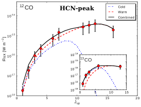
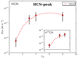
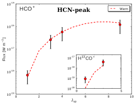
Figure 14: Two component fit of the line spectral energy distribution of the CO, HCN, and HCO⁺ species, for the spectra at position ($-65^{\prime\prime}$,$+31^{\prime\prime}$) toward the HCN-peak. The fit of the ¹³C bearing isotopologues is shown in the insets. The cold and warm components are shown in dashed and dotted lines, respectively. The error bars are as in Fig. 9.

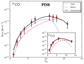
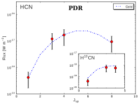
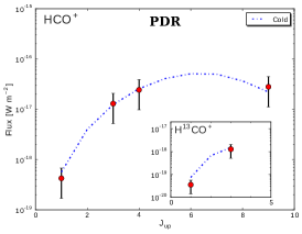
Figure 15: Two component fit of the line spectral energy distribution of the CO, HCN, and HCO⁺ species, for the spectra at position ($-60^{\prime\prime}$,$-30^{\prime\prime}$) toward the southern PDR. The fit of the ¹³C bearing isotopologues is shown in the insets. The cold and warm components are shown in dashed and dotted lines, respectively. The error bars are as in Fig. 9.

Table 16: LSED fit parameters for the spectra toward the HCN-peak position ($-65^{\prime\prime}$,$+31^{\prime\prime}$).

Parameter	CO	HCN	HCO+
$\Phi_{cold}(^{12}{\rm C})$	0.90 $\pm$ 0.09
$n_{cold}(\rm H_{2})$ [cm-3]	4.50 $\pm$ 0.43
$T_{cold}$ [K]	40.00 $\pm$ 4.52
$N_{cold}$ [cm-2]	19.40 $\pm$ 1.10
$\Phi_{warm}(^{12}{\rm C})$	0.35 $\pm$ 0.04	0.35 $\pm$ 0.04	0.35 $\pm$ 0.02
$n_{warm}(\rm H_{2})$ [cm-3]	6.00 $\pm$ 0.63	6.00 $\pm$ 0.42	6.00 $\pm$ 0.32
$T_{warm}$ [K]	130.00 $\pm$ 9.62	130.00 $\pm$ 14.11	130.00 $\pm$ 15.78
$N_{warm}$ [cm-2]	18.40 $\pm$ 0.33	15.10 $\pm$ 0.39	14.90 $\pm$ 0.34
$\Phi_{cold}(^{13}{\rm C})$	0.90 $\pm$ 0.10
$\Phi_{warm}(^{13}{\rm C})$	0.35 $\pm$ 0.03	0.35 $\pm$ 0.04	0.35 $\pm$ 0.03
$\Delta V(^{12}{\rm C})$ [km s${}^{-}1$]	4.60	7.50	6.00
$\Delta V(^{13}{\rm C})$ [km s${}^{-}1$]	3.50	3.90	3.70

Table 17: LSED fit parameters for the spectra toward the southern PDR position ($-60^{\prime\prime}$,$-30^{\prime\prime}$).

Parameter	CO	HCN	HCO+
$\Phi_{cold}(^{12}{\rm C})$	0.90 $\pm$ 0.07	0.35 $\pm$ 0.04	0.35 $\pm$ 0.04
$n_{cold}(\rm H_{2})$ [cm-3]	5.50 $\pm$ 0.60	5.30 $\pm$ 0.51	5.30 $\pm$ 0.55
$T_{cold}$ [K]	60.00 $\pm$ 8.21	60.00 $\pm$ 7.01	60.00 $\pm$ 6.16
$N_{cold}$ [cm-2]	18.80 $\pm$ 0.67	16.00 $\pm$ 0.56	15.50 $\pm$ 0.53
$\Phi_{warm}(^{12}{\rm C})$	0.20 $\pm$ 0.03
$n_{warm}(\rm H_{2})$ [cm-3]	5.80 $\pm$ 0.52
$T_{warm}$ [K]	110.00 $\pm$ 10.18
$N_{warm}$ [cm-2]	18.60 $\pm$ 1.37
$\Phi_{cold}(^{13}{\rm C})$	0.90 $\pm$ 0.12	0.35 $\pm$ 0.04	0.35 $\pm$ 0.04
$\Phi_{warm}(^{13}{\rm C})$	0.20 $\pm$ 0.02
$\Delta V(^{12}{\rm C})$ [km s${}^{-}1$]	4.30	5.00	4.50
$\Delta V(^{13}{\rm C})$ [km s${}^{-}1$]	4.30	3.80	3.90