Further constraints on the optical transmission spectrum of HAT-P-1b

Abstract

We report on novel observations of HAT-P-1 aimed at constraining the optical transmission spectrum of the atmosphere of its transiting Hot-Jupiter exoplanet. Ground-based differential spectrophotometry was performed over two transit windows using the DOLORES spectrograph at the Telescopio Nazionale Galileo (TNG). Our measurements imply an average planet to star radius ratio equal to R_p/R_∗=(0.1159$\pm$0.0005). This result is consistent with the value obtained from recent near infrared measurements of this object but differs from previously reported optical measurements being lower by around 4.4 exoplanet scale heights. Analyzing the data over 5 different spectral bins $\sim$600Å  wide we observed a single peaked spectrum (3.7 $\sigma$ level) with a blue cut-off corresponding to the blue edge of the broad absorption wing of sodium and an increased absorption in the region in between 6180-7400$\rm\AA$. We also infer that the width of the broad absorption wings due to alkali metals is likely narrower than the one implied by solar abundance clear atmospheric models. We interpret the result as evidence that HAT-P-1b has a partially clear atmosphere at optical wavelengths with a more modest contribution from an optical absorber than previously reported.

1 Introduction

The possibility to characterize transiting exoplanet atmospheres by means of high precision spectrophotometric measurements acquired during transits was theorized in a few works early this century (Seager & Sasselov 2000; Brown 2001). The light of the hosting star, filtered by the planeary atmosphere in the terminator region is absorbed and scattered by chemical compounds so that, once observed at different wavelenghts, the atmosphere may appear more or less opaque to the observer. Hence, transit depth determinations obtained in different spectral domains can be used to reconstruct a low resolution spectrum of the planetary atmosphere.

Models predict that atmospheres of cloud free hot-jupiter planets should be dominated in the optical by broad absorption features of the alkali metals Na and K. Studies so far have revealed a certain diversity of atmospheric features. Sodium was first detected by Charbonneau et al. (2002) in the atmosphere of HD209458b using the STIS spectrograph on board of HST and later on confirmed also by ground based observations (Snellen et al. 2008). Subsequent studies have revealed the presence of alkali metals also in the atmospheres of other planets, for example sodium was detected in WASP-17b (e. g. Wood et al. 2011; Zhou & Bayliss 2012) and HAT-P-1b (Nikolov et al. 2014) while potassium has been detected in XO-2b (Sing et al. 2011), WASP-31b (Sing et al. 2015) and HAT-P-1b (Wilson et al. 2015). The atmosphere of other planets seem to be obscured by clouds or hazes, as in the case of WASP-12b (Sing et al 2013) and HD189733 (Pont et al. 2013), albeit for this planet narrow line cores of sodium were also found (Redfield et al. 2008; Huitson et al. 2012; Jensen et al. 2012).

Near infrared studies have soon complemented analysis conducted in the optical domain, particularly exploiting the Spitzer Space Telescope and lead to the conclusion that close-in extrasolar planets could be broadly subdivided in two big categories according to the structure of their temperature-pressure profile (Hubeny et al. 2003; Fortney et al. 2006, 2008; Burrows et al. 2007, 2008). The pM class planets show a high altitude temperature inversion in their atmospheres whereas the pL class planets do not, resulting in different emergent spectral energy distributions in the near infrared domain and different spectral signatures (like the flipping of water bands from absorption to emission passing from non inverted to inverted atmospheres). The origin of such inversion is identified with the absorption of strong stellar irradiation in the optical domain by a variety of possible absorbers (Fortney et al. 2010, Burrows et al 2007, Zahnle et al. 2009).

The present study is focussed on HAT-P-1b, one interesting member of the family of hot-jupiter planets. HAT-P-1b is a low mean density ($\rho\rm_{p}\,\sim\,$0.35 g cm^-3) giant exoplanet (R$\rm{}_{p}\,\sim\,$1.2 R_J) discovered by the HATNet transit survey (Bákos et al. 2007). The host star ($V=$10.4) is a member of a visual binary system with the two components separated by around 11^″ on the sky ($\sim\,1500$ AU). Both are G0V stars and the companion star is around half a magnitude brighter than the target in the $V$ filter. The low density of the exoplanet, the brightness of the host star, and the presence of a close-by stellar companion make HAT-P-1b an ideal target for follow-up studies aiming at characterizing its atmosphere using transmission spectroscopy. In particular, the close stellar companion can be used to correct for systematic effects performing simultaneous differential spectrophotometric measurements of the two stars.

HAT-P-1b is an interesting object also in the context of inverted atmosphere theory. The pM/pL transition is set in correspondence of the TiO condensation limit (Fortney et al. 2008), and HAT-P-1b would sit just at the lower edge of this limit providing an important benchmark test for theory. Todorov et al. (2010) obtained Spitzer/IRAC photometry for this object and concluded that the observations were best fitted using an atmosphere with a modest temperature inversion, and that the planet has a strong day/night contrast ratio implying little energy redistribution.

Three studies have been presented so far discussing the atmosphere of HAT-P-1b by means of transmission spectroscopy. Wakeford et al. (2013) presented HST Wide Field Camera 3 (WFC3) near-infrared transmission spectroscopy detecting a significant absorption above the 5-$\sigma$ level matching the 1.4 $\mu$m water absorption band, and concluding that a 1000 K isothermal model or a planetary-averaged temperature model best matched the observations. Nikolov et al. (2014, hereafter N14) presented HST/STIS optical transmission spectroscopy implying a strong absorption shortward of 5500Åand possibly redward of 8500Å, as well as sodium absorption at a 3.3$\sigma$ level, but no evidence for potassium absorption. Interestingly, the same authors observed that STIS and WFC3 spectra differ significantly in absolute radius level (4.3$\pm$1.6 pressure scale heights). On the basis of their analysis N14 suggested the presence of a strong $extra$-optical absorber and of a super-solar (factor 10³) sodium to water abundance ratio to explain this result. This absorber would partially block the sodium wings and completely mask the potassium feature, yet leaving immuted the 1.4$\mu$m absorption band. Later Wilson et al. (2015) detected potassium in the atmosphere of this planet (albeit at a much higher resolution than N14) using the GTC telescope in narrowband imaging and employing the flexible red tunable filters technique. To explain the amplitude of the detected feature the authors hypothesized that high-temperatures at the base of the upper atmosphere may result in an increased scale height, and/or suggested that a lower mean molecular weight could be present caused by the dissociacion of molecular hydrogen into atomic hydrogen by EUV flux from the host star.

In this work we present novel ground-based transmission spectroscopy measurements for two full transit events of HAT-P-1b obtained with the Telescopio Nazionale Galileo (TNG) and the low resolution spectrograph DOLORES (Device Optimized for the LOw RESolution). Our data cover the spectral range between $\sim$4900Å  and $\sim$8000Å, and were obtained between August and October 2012.

Our observations are presented in Sect.2, in Sect.3 we review our data analysis technique, in Sect.4 we present the study of the transit lightcurves, in Sect.5 we discuss the results and in Sect.6 we summarize and conclude.

2 Observations

We observed two full transits of HAT-P-1b in August 14, 2012 and in October 20, 2012. The data were collected with DOLORES, the low resolution spectrograph and camera installed at the Nasmyth B focus of the TNG. The camera is equipped with a 2100 x 2100 E2V 4240 Thinned back-illuminated, deep-depleted, Astro-BB coated CCD with a pixel size of 13.5 $\mu$m corresponding to a pixel scale of 0.252 arcsec/pix. The CCD gain factor is 0.97 e^-/ADU while the readout noise is around 9 e^- RMS. We used the LR-B grism providing a dispersion of 2.52 Å/pix and adopted a slit width of 10 arcsec. The resolution was therefore seeing limited. An average seeing of 0.8 arcsec was measured at the center of our spectral window implying a resolution of 8 Å  or a resolving power equal to 625 at 5000 Å. During both nights observing conditions were clear.

Overall we observed uninterruptedly for 5.1 hours during the first night and for 5.3 hours during the second. Before starting the scientific exposures we obtained bias, flat field, calibration lamp spectra and a telluric standard star with the same instrumental setup described above.

We adopted a slit position angle equal to 72.62 degrees in order to place the target star and its close-by companion on the slit and kept this configuration for the entire observing runs.

Exposure time was set to 12 sec with a read out time equal to 45 sec during the first night and to 12 sec during the second. This was a consequence of windowing the detector during the second night of observation. A summary of the observations can be found in Table 1.

3 Data analysis

The data reduction was performed with our own customised software. After applying bias correction and flat-fielding we determined the extraction region for both the target and comparison star spectra. Along the dispersion direction ($x$ axis) the extraction region was fixed between 970 pix up to almost the end of the detector (2060 pix) that is between $\sim$4900Åand $\sim$8000Å. Along the spatial direction we considered an extraction window including both spectra (which were separated by around 44 pix on the detector) and an additional 30 pix region on the top and the bottom to properly measure the sky. We then calculated the spectral centroids and the full width half maximum (FWHM) separately in each column by fitting a bi-gaussian analytic function with exponential wings. The PSF profile is slightly asymmetric and for this reason we adopted a bi-gaussian function for the central core of the PSF. Moreover, the PSF is also more extended than a simple gaussian and the exponential wings provided a more accurate approximation. Both profiles were fit simultaneously, while the sky was first measured in the outermost regions and then fixed throughout the process.

3.1 Cosmic rays correction

To remove the cosmic rays contaminating our data, we shifted and rescaled the spatial profile of each column into an average PSF by means of the analytical solution determined previously. We then spline interpolated the PSF at 1/10th pixel resolution shifting and rescaling backward this empirical PSF to the position of each column profile. We integrated numerically the PSF over 1 pix to match the detector resolution. We measured the scatter around the average PSF, and took a generose threshold of 20 times this value with respect to the shifted and rescaled PSF to isolate possible outliers in the column profiles. Once an outlier was found we replaced its value with the model PSF value. On average we measured 1-2 cosmic events per image.

3.2 Extraction

The flux of each star was extracted from the measured centroid position in each column into an aperture of 12 px radius by using aperture photometry. The aperture radius was chosen after experimenting different apertures taking the one that provided the highest precision in the final photometry.

3.3 Wavelength drift correction

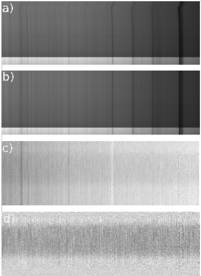
Figure 1: This Figure highlights the major steps in the reduction chain. For each panel, dispersion direction is along the x axis. Each line represents a spectrum obtained at a given epoch. Spectra are chronologically ordered from the bottom to the top of each panel. Data are relative to the first night of observation. a): Observed spectra of the target star b) spectra are re-aligned to the same wavelenght reference system c) residual spectrum after dividing each target spectrum to the correspondent comparison star spectrum d) differential atmospheric extinction correction.

After extracting the flux from each spectrum we constructed bidimensional maps of dispersion versus time flux variations. In these maps each line represents a spectrum of the target (or the comparison) at a given epoch. In Fig. 1 (top panel), we show the target map obtained just after flux extraction for the first night of observation. As is evident from the deepest absorption lines visible in the spectrum, the spectra shifted along the dispersion direction during the night. The maximum shift was equal to 1.7 arcsec (with respect to the initial position) during the first night and equal to 4 arcsec during the second. In both cases both the star and the comparison remained always well within the slit thanks to the adoption of a large aperture. Before lightcurve construction it is important to realign the spectra and bring them to the same reference system. We used the out of transit measurements to construct an average spectrum of the target and of the comparison star, which was obtained by scaling the spectra at mid-wavelength and averaging their profiles. We used then a deep absorption line to obtain a first guess of the shift between the single spectra and the average spectrum from the difference of the minimum. Then we cross-correlated the splined interpolated average spectrum to each single spectrum over a region of 2 pix around the initial guess, and at a step of 1/10th of a pixel. Finally we spline interpolated the orginal spectrum at half of a pixel and shifted them accordingly to the best value of the shift obtained by the cross-correlation. The result is shown in Fig 1 (second panel from the top). This procedure was applied independently both for the target and comparison spectra.

3.4 Normalization to the comparison spectrum

We procedeed by dividing the target spectra by the comparison spectra, obtaining the flux ratio of the two. This division was applied to each pixel of the bidimensional maps reported above. The result is illustrated in Fig. 1 (third panel from the top). All but the some absorption lines in the original spectra disappear by forming the flux ratios, demonstrating the effectiveness of the adoption of the comparison star. The horizontal dark band visible in all images corresponds to the transit event.

3.5 Differential atmospheric extinction correction

One of the big advantages of differential spectrophotometry over normal differential photometry is the possibility to model and remove more accurately the effect of our own atmosphere. The flux ratio map presented above displays both a continuous atmospheric differential extintion between the target and the comparison, and also some localized differential absorption. To further improve the result, we then applied a wavelength dependent differential atmospheric extinction correction to each single detector column. We adopt a linear model for the flux variation as a function of airmass and fit it to each column of the flux ratio maps by using only out of transit data. We then normalized each column by the model solution. The result is shown in Fig 1 (fourth panel from the top) and demonstrates that also the residual contamination is well removed by this approach.

3.6 Uncertainties

To each flux measurement we associated an uncertainty based on the following theoretical formula:

$$\rm\frac{\Delta\,F\,}{F}=\,\sqrt{\sigma F_{0}^{2}+\sigma F_{s}^{2}}$$ (1)

with

$$\rm\sigma F_{0}=\frac{\sqrt{F+RON^{2}+\frac{\sigma_{sky}^{2}}{N_{sky}}}}{F}$$ (2)

$$\rm\sigma F_{s}=0.09\,\frac{D^{-\frac{2}{3}}\,A^{1.75}\,\rm e^{-h/8}}{\sqrt{2\,T_{exp}}}$$ (3)

where F corresponds to photon counts within the aperture, RON is the detector read out noise, $\rm\sigma F_{0}$ is the photon and instrumental noise, $\rm\sigma_{sky}$ is the uncertainty in the mean sky determination (in photons) and $\rm N_{sky}$ is the number of pixels from which the sky was determined. $\rm\sigma F_{s}$ is the scintillation noise which we estimated using the formula reported in Gilliland et al. (1993) based on the work of Young et al. (1967) and where D is the telescope diameter in cm, A the airmass, h the altitude of the observatory in km and T_exp the exposure time in seconds.

Eq. 1 was used to construct dispersion versus time bidimensional uncertainty maps which were associated with the scientific measurements described in previous sections.

3.7 Estimates

During our observations we acquired around 9.7$\times$10⁷ total photons per exposure for the comparison star and 5.6$\times$10⁷ photons for the target. Pure photon and detector noise would imply a precision of 0.013$\%$ per measurement, scintillation calculated from the above formula would add the non-negligible contribution of 0.027$\%$ at low airmasses, depending quite sensibly on the airmass. We can expect a total error budget of around 0.03$\%$, that is around 300 ppm. The resulting precision on the transit depth determination can be estimated by considering the error on the mean levels of the in and out of transits measurements. For the first and second night we obtain an estimate of around 0.003$\%$ and 0.002$\%$.

Assuming as in N14 that a scale height of HAT-P-1b is equal to 414 km, this corresponds to a required photometric precision in the transit depth determination equal to 0.012$\%$ (or around 0.0005 in the radius ratio determination). The error estimate reported above does not account for some other complications present in the transit fit process, like for example the necessity to model the limb darkening. What it demonstrates, however, is that photon noise is not the limiting factor in this experiment. Even rebinning the measurements into few spectral bins we should be able to remain confortably below the limit imposed by one scale height. The real challange is to maintain the accuracy of the measurements down to this level of precision. For ground based observations this also means to accurately remove the contribution of our own atmosphere.

3.8 Contamination

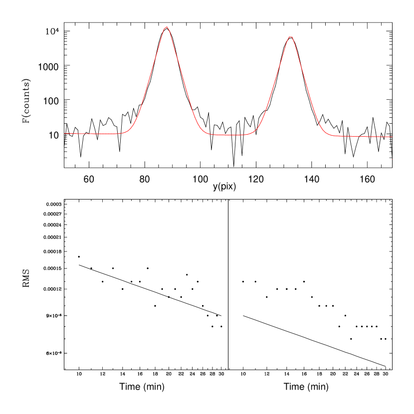
Figure 2: Top panel: spatial cut of a typical spectrum at mid-wavelentgth showing both the comparison star and the target. The red continuous line denotes our best-fit model. Note the logarithmic scale on the y-axis. Bottom panels: theoretical RMS (continuous line) against observed RMS (points) as a function of temporal binning. On the right white lightcurve results from the first night, and on the left for the second night.

In Figure 2 (top panel), we show the profile of the comparison and target star along the spatial direction, as observed at mid-wavelength for a typical spectrum. The y-scale is logarithmic to enhace the visibility of the PSF wings. This Figure demonstrates that the two objects are well separated in our images. The aperture radius we adopted is around 4.6 times the measured fwhm. The centroid of the target star is distant around 17 fwhm from the centroid of the comparison. Considering our best fit analytic model (denoted in red in the figure) this implies that the flux of the comparison integrated across the target aperture is entirely negligible (nominally at a level of 10^-12 the target flux).

3.9 Masking

For some isolated measurements we noted that errors were appreciably different from the average. These situations were probably associated with image artifacts and/or cosmics not perfectly corrected by our automatic pipeline. To mask these regions we adopted an iterative 5-$sigma$ clipping algorithm measuring the average uncertainty and the scatter inside a 10px box radius window scanning the entire dispersion-time domain. Overall, the fraction of measurements masked this way was equal to $\sim$0.05$\%$ of the total number of bins.

3.10 Wavelength calibration

We used a Ne+Hg lamp obtained just before starting the scientific sequence to map pixels into wavelength, in angstroms. The lamp was observed with the same grism, but with a smaller slit width of 2 arcsec to allow a better identification of the spectral lines.

4 Lightcurve analysis

Lightcurves were obtained by calculating a weighted average of the flux ratios in different spectral channels. At first, to fix the global system parameters, we simply averaged the measurements over all the spectral range of our spectra. The resulting lightcurve is usually referred to as $white$ lightcurve.

4.1 White lightcurves

White lightcurves were produced and analyzed independently for each night of observation. We assumed a perturbed transit model. As long as systematics are small as compared to the transit it is always possible to express the global model (transit with systematics) as a sum of an unperturbed transit model (F_MA) which is given in this case by the Mandel & Agol (2002) formula and a correcting term which is express below as a linear combination of different systematic components:

$$\rm F(t)=F_{MA}(t)+c_{1}\,\times\,Air(t)+c_{2}\times\,xc(t)+c_{3}\times\,s(t)+c_{4}$$ (4)

where c₁,c₂ and c₃ are three parameters to account for residual flux losses related to airmass (Air), spectral shifts along the dispersion direction (xc) and seeing (s). The constant c₄ accounts for a photometric zero point offset.

We applied the Bayesan Information Criterium (BIC) to determine the best model to fit the data considering different combinations of the above parameters. For the first night of observation the model reported in Eq. 4 was the favoured one, for the second night the BIC analysis indicated that the seeing dependence could be dropped and we thereby fixed c₃ to zero.

For the planet-to-star normalized distance we adopted the parameterization described in Montalto et al. (2012) and therefore fit a maximum of nine free parameters: the time of transit minimum ($T_{0}$), the planet to star radius ratio ($r$), the total transit duration ($T_{14}$), the mean stellar density ($\rho_{\star}$), the linear limb darkeneing coefficient ($g1$) and the four coefficients c₁, c₂, c₃ and c₄.

We fitted each lightcurve with the Levemberg-Marquardt algorithm (Press 1992) using the partial derivatives of the flux loss calculated by Pál (2008) as a function of the radius ratio $r$ and the normalized distance $z$ to calculate the differential corrections to apply to each parameter at each iterative step.

We assumed a quadratic limb darkening law where the quadratic coefficient ($g2$) was obtained (and thereby fixed) using the software developed by Espinoza & Jordán (2015) adopting the ATLAS model atmospheres results and plugging in the response function of the TNG+LRS intrument. The quadratic coefficient was calculated in this way both for the white lightcurves and for the different band lightcurves. HAT-P-1A spectroscopic parameters were obtained from the SWEET-Cat catalog (Santos et al. 2013): $\rm T_{eff}=(6076\,\pm\,27)\,K$, $\rm lg_{LC}(g)=4.40\,\pm\,0.01$, [Fe/H]=$+0.21\,\pm\,0.03$ and $\rm v_{t}=(1.17\,\pm\,0.05)\,km\,s^{-1}$. We also calculated in the same way the value for the linear coefficient $g1$ and used this value as initial guess for this parameter. The initial guesses for the other system parameters ($T_{14}$, $r$, $\rho_{star}$) were obtained from the analysis of N14 as reported in their Table 5, whereas for the slope parameters c₁, c₂, and c₃ we assumed simply zero as initial guess and for the constant c₄, instead, one.

For the orbital period we first adopted the value reported by N14 and derived the time of transit minimum T₀ for our transits using the Levemberg-Marquardt algorithm described below. We therefore used transit timings reported in the literature to further refine the value of the reference transit time T₀ as well as the orbital period P adopting a linear ephemerides

$$\rm T_{C}(E)\,=\,T_{0}\,+\,E\,\times\,P,$$ (5)

where T_C(E) is the time of transit minimum at epoch E. We obtained T₀=(2453979.9321$\pm$0.0003) days and P=(4.46529961$\pm$0.00000071) days with a reduced chi equal to $\chi_{r}=1.35$. In Table 2 we report the list of transit times we used in this calculation.

We used the Levemberg-Marquardt algorithm (Press 1992) to obtain an initial solution for the free parameters. For each iteration the the reduced $\chi_{red}$ of the fit was calculated

$$\rm\chi_{red}\,=\,\sqrt{\sum_{i=1}^{i=N}\frac{(O_{i}-F_{i})^{2}}{N-N_{free}}}$$ (6)

where $\rm O_{i}$ is the observed flux corresponding to the i-th measurement, $\rm F_{i}$ is the model calculated flux as described above, $\rm N$ is the total number of measurements, and $\rm N_{free}$ the number of free parameters. The Levemberg-Marquardt algorithm delivered the best solution by means of $\rm\chi_{red}$ minimization.

4.2 Correlated noise

To each photometric measurement we associated an error equivalent to the error of the weighted average over integrated passband as derived from our uncertainty maps. These errors were rescaled so that the best models gave as result $\rm\chi^{2}$=1. The presence of correlated noise in the data limits the precision of the observations (Pont et al. 2006). We then compared the RMS of the fit residuals averaged over M bins with the theoretical prescription valid for uncorrelated white noise

$$\rm\sigma_{M}=\frac{\sigma}{\sqrt{N}}\,\sqrt{\frac{M}{M-1}}$$ (7)

where N is the total number of residuals and $\sigma$ is the RMS of all residuals. We considered bin sizes comprised in between 10 min to 30 min. The average ratio ($\beta$) of the measured dispersion to the theoretical value was taken as a measurement of the degree of correlation in the data, and the uncertainty were then globally expanded by this factor. We found that the $\beta$ parameter was in between 1.05 and 1.62.

In Figure 2 (bottom panels), we show the thoretical RMS (continuous line) and the observed RMS (points) as a function of the binning timescale for the first and the second night white lightcurves (left and right respectively). In both cases residuals are scaling down quadratically with rebinning time though, over the analyzed timescales, the second night appears to be more affected by red noise ($\rm\beta=1.4$) than the first ($\rm\beta=1.1$).

4.3 Monte carlo analysis

Subsequently we performed a Markov Chain Monte Carlo analysis as described in Montalto et al. (2012) to refine the estimate of the uncertainties. We considered 200000 iteration steps and 10 chains for each lightcurve, merging then the resulting chains after dropping the first 20$\%$ burn-in phase iterations.

The results are illustrated in Fig. 3 and the corresponding best-fit parameters are reported in Table 3. The RMS of the white lightcurves residuals is 525 ppm for the first night and 462 ppm for the second night.

4.4 Multi-band lightcurves

We experimented various subdivisions of our spectral window into different spectral bins trying to optimize the resolution of the final spectrum while keeping the precision of the transit depth determination at a level of around one scale height. Finally we adopted the a subdivision into five $\sim$600Å  wavelength bins. A common mode systematic model derived from the white lightcurves was subtracted from the multi-band lightcurves. The analysis reported above was then repeated for each lightcurve. In this case we fixed the stellar density, time of transit minimum and total transit duration to the average values (of the two nights) derived from the white lightcurve analysis. This assumption is justified by the fact that we do not expect these parameters to be wavelength dependent. The results are then illustrated in Fig. 3 and reported in Table 4.

5 Results

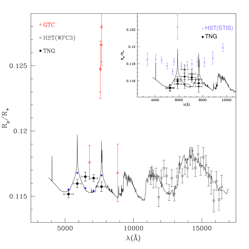
Figure 4: Comparison between different transmission spectroscopy measurements of HAT-P-1b and theoretical model predictions. In the main plot black circles denote TNG measurements presented in this work, grey boxes HST(WFC3) measurements (Wakeford et al. 2013), red triangles GTC measurements (Wilson et al. 2015). The model depicted is calculated for a solar abundance of Na and K. Blue asteriscs indicate model predictions averaged over TNG bandwidths. In the box on the top right, close-up view of the optical region displaying the HST(STIS) measurements (slate blue crosses, N14) and TNG measurements black circles. Open symbols denote single epoch TNG measurements (circles for the first epoch, boxes for the second). The same model displayed in the main figure is also presented.

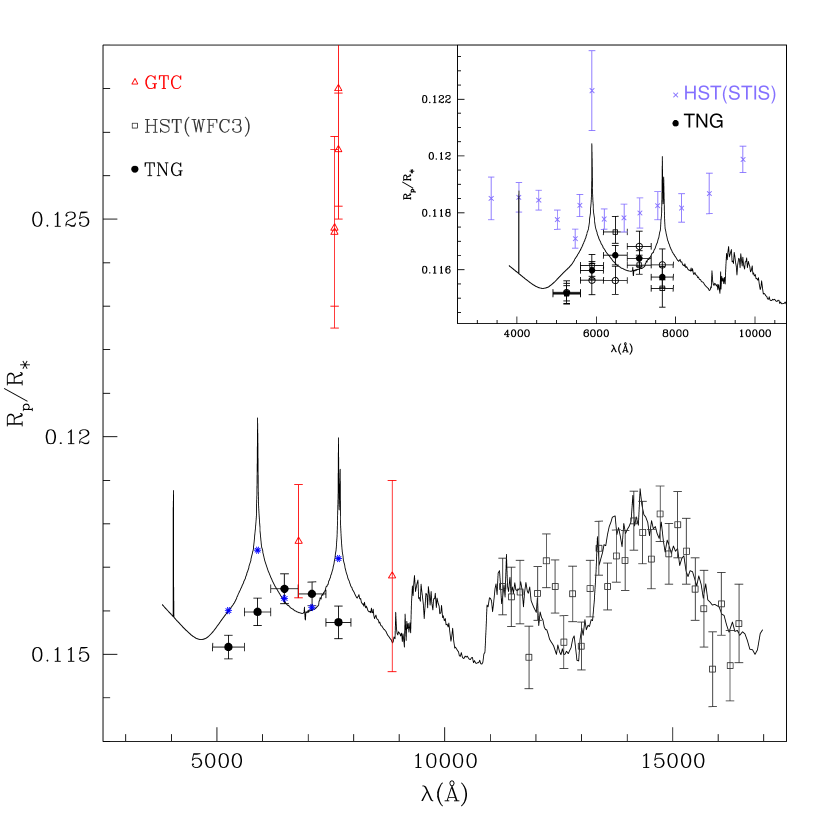
Figure 6: The same as Figure 3 with a model calculated for a supersolar (10$\rm\times$) abundance of Na and K.

In Fig. 4 to Fig. 6 we present the results of our analysis. The black points denoting our final spectrum were obtained by taking the weighted average of the results of both observing nights as reported in Table 5.

A fit with a constant line to our data returns a $\chi_{red}=$1.9 which may appear a bit high. The morphological structure seems to indicate a single peaked spectrum. A fit with a quadratic model renstitutes a peak around 6650 Å, close to the red edge of the third bin. The measurement with the lowest radius ratio appears to correspond to the bluest bin. Averaging the measurements braketing the peak in the third and fourth bin and forming the difference with the bluest bin we get a S/N equal to 3.7. Further insights into the characteristics of this spectrum and its physical plausibility can be obtained by comparing these results with the predictions of planet atmosphere models.

In order to compute the synthetic spectra, we use line-by-line radiative transfer calculations from 0.3 to 25 $\mu$m. The model is fully described in Iro et al. (2005) and Iro & Deming (2010).

As opacity sources we include the main molecular constituents: H₂O, CO, CH₄, CO₂ , NH₃ (the latter two are added with respect to the previous references, taken respectively from Rothman et al. 2009, 2010), Na, K and TiO; Collision Induced Absorption by H₂ and He; Rayleigh diffusion and H^- bound-free and H${}_{2}^{-}$ free-free. The current model does not account for clouds.

In the nominal model, we assume the atmosphere is in thermochemical equilibrium with a solar abundance of the elements. We generated also two additional models with ten times higher and lower abundances of Na and K with respect to the solar value.

Planet and star parameters are taken from N14. As input heating we use a stellar spectrum computed from Castelli & Kurucz (2003) for a G0V star with an effective temperature of 6000K.

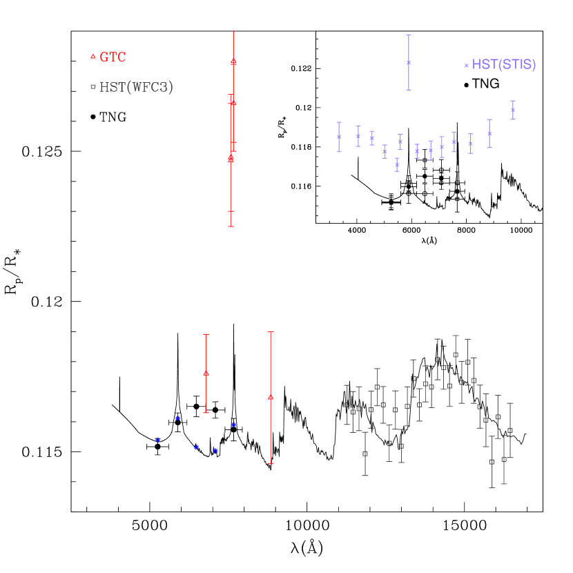
Figure 5: The same as Figure 3 with a model calculated for a subsolar (10$\rm\times$) abundance of Na and K.

The comparison of the models with the global set of transmission spectroscopy measurements of HAT-P-1b acquired so far is illustrated in Fig. 3-Fig. 5.

The models were fitted to the near infrared data of Wakeford et al. (2013) and then simply projected in the optical. We then calculated the reduced $\chi_{r}$ of the models (averaged over the TNG bandwidths) with respect to the TNG measurements. The results indicate that for all cases considered a poor fit is obtained. In particular, the solar abundance model displayed in Fig. 3 implies $\chi_{r}=$2.9, the super-solar model (Fig. 5) $\chi_{r}=$3.4, and the sub-solar model (Fig. 4) $\chi_{r}=$3.2. A closer look at these results suggest that clear models could be able to fit a portion of the obtained spectrum, but not the whole spectrum. In particular, the subsolar model appears to be able to perfectly reproduce the blue edge cut-off of the sodium line, as well as the sodium and potassium region. Restricting the analysis to these bins we would obtain $\chi_{r}=$0.7 for this model. The discrepancy in the region in between Na and K is however quite remarkable (at the level of 6.3 $\sigma$). This result could be interpreted as evidence that the broad wings of alkali metals in the HAT-P-1b atmosphere are narrower than what implied by the standard solar model. Moreover, it suggests that to be able to reproduce the entire spectrum it is necessary to assume an extra absorption in the region in between Na and K.

The plausibility of this hypothesis can be verified considering also previous observational results and the comparison with theoretical models which include the contribution of extra absorbers.

In particular our result appears similar to the case of HD209458b. Desért et al. (2008) found that for this planet the blue side of the sodium wing was well defined but an increased absorption was observed redward of it. They suggest that the increased opacity could be explained by the presence of a weak absorption from TiO/VO clouds, implying the presence of a modest temperaure inversion in the atmosphere. In the case of HAT-P-1b it seems that the absorption is more extended toward the red than in the case of HD209458b. It is also worth noting, however, that new analysis of near infrared data appear to not confirm early claims on the existence of a temperature inversion in HD209458b (Diamond-Lowe et al. 2014, Evans et al. 2015).

For the case of HAT-P-1b secondary eclipse measurements in the IRAC/Spitzer bands lead to the conclusion that HAT-P-1b appears to have a modest thermal inversion (Todorov et al. 2010). Our optical spectrum may therefore support this conclusion, and it could help to identify the optical counterpart of the opacity source that produces the observed infrared exess. We note that the same authors derived a dayside temperature of 1550$\pm$100 K (assuming zero albedo and no heat redistribution). This temperature appears quite low to attribute our peak absorption to TiO/VO clouds, given that these compounds are expected to condense below 1600 K but we note that also other potential absorbers have been proposed (Burrows et al. 2007, Zahnle et al. 2010).

In conclusion, our optical observations of HAT-P-1b suggest that the planet has a partially clear atmosphere with a modest absorption from clouds (or other absorbers) concentrated in the region in between 6180-7400 Å.

5.1 Impact of model assumptions

In this subsection we investigate the dependence of our results on several assumptions that have been considered during our analysis.

First of all, as reported in the previous sections, during our analysis we considered a semi-empirical approach to model limb-darkening and adopted a quadratic limb-darkening law. Quadratic approximation is usually sufficient to describe transit lightcurves considering the actual precisions of observational data. However other authors, like for example N14, prefer to dopt a four coefficient law setting the coefficients to theoretical values. A four coefficient law is expected to reproduce more accurately the radial flux distribution across the stellar disk, in particular at the limb (e. g. Claret & Bloemen 2011). We tried then to investigate the possible dependence of our results on the adopted limb-darkening law. We therefore considered a four coefficients limb-darkening law and replicated the procedure reported above setting the coefficients to the values obtained by using the software of Espinoza & Jordán (2015) considering our white lightcurve passband and the response function of our instrumentation. This procedure delivered the values (0.5884,-0.0445,0.3287,-0.1984) for the four coefficients in increasing order of power. Additionally, in order to reproduce more closely the analysis of N14 we also fixed the stellar density and the transit duration to the exact values reported by N14. We note however, that the stellar density we derived is consistent within 0.75 $\rm\sigma$ and the transit duration within 1.8 $\rm\sigma$ with respect to the values reported by N14. The result of this analysis implies a radius ratio equal to (0.1161$\pm$0.0003) for the first night white lightcurve and equal to (0.1160$\pm$0.0004) for the second night white lightcurve. This test therefore further supports our conclusion on the presence of a largely clear atmosphere in HAT-P-1b.

We also tested the adoption of a different mathematical formulation for the systematic model analysis. In particular, we considered as in Stevenson et al. (2014) a model where the systematic terms are factorized rather than summed to the unperturbed transit model. Each systematic term is then assumed of the form (1+$a\,\times\,$x) where $a$ is a modulating factor and x is the normalized (mean subtracted) variable describing a given systematic (airmass, seeing, etc.). Expressing the model in this way should reproduce more closely the physical mechanisms underlying the systematic flux variation. Given the small amplitude of systematics in our data this formulation produced results which are fully consistent with the perturbed transit model analysis described above. In particular, for the white lightcurves transit depths we obtained (0.1149$\pm$0.0008) and (0.1164$\pm$0.0007) for the first and second nights respectively, that is well within our quoted uncertainties. This result then supports our analysis and adopted formulation for systematics modeling.

5.2 Discussion

While we concluded that clouds (or extra absorbers) are necessary to explain the spectrum of HAT-P-1b, they overall impact seems to be substantially smaller than the one reported by N14, as also shown in the top right corners of Fig. 3-Fig. 5.

In the next subections, we investigate three possible mechanisms that could be at the origin of the observed difference between our optical results and the one presented in N14.

5.3 Stellar activity

Stellar activity is a known phenomenon that can produce radius ratios variations (e. g. Oshagh et al. 2014). HAT-P-1b is not regarded an active star. A very low chromospheric activity in the CaII and K lines has been measured (Bakos et al. 2007; Knutson et al. 2010) with log(R’_HK)=-4.984. Transit follow-up analysis (including this work) did not show evidence of spot crossing events. In addition to that, photometric monitoring was conducted at the Liverpool Telescope between 2012 May 4 and 2012 December 13, covering all the HST visits during which HAT-P-1b was observed as presented in N14. Because our measurements have been acquired in August and October 2012, the photometric constraints derived by the authors apply also to our case. The Liverpool Telescope follow up implied that HAT-P-1A was not variable during the observing period down to a precision of around 0.2$\%$ as we can infer from N14 (Figure 2). Visit 20 of HST observed with the G750 grism (overlapping our spectral window) and produced a radius ratio equal to R_p/R_s=0.11808$\pm$0.00034. Our average radius ratio is R_p/R_s=0.11590$\pm$0.0005. Squaring these two radius ratio estimates and taking their difference we obtain an expected level of photometric variability around 0.05$\%$. Such a value is around four times smaller than the precision reached by the Liverpool Telescope. This calculation shows that probably it is premature to completely rule out stellar variability as a potential source of systematic variation of the radius ratio. In particular it results that the observed radius ratio difference could be produced if a sub-millimag variability is present.

5.4 Exo-weather

Although in the previous section we argued that the current photometric constraints are not very tight to completely rule out the stellar variability hypothesis, the level of variability required to explain the radius variation appears indeed quite small. Assuming for HAT-P-1b an atmospheric scale height of 414 km as in N14, this implies that the observed difference would amount to around 4.4 scale heights. Atmospheric effects produced in the atmosphere of the exoplanet may be present over a range of a few scale heights so that it is interesting to speculate on the possibility that the observed radius ratio difference may be produced by a mechanism which has its origin in the atmosphere of the planet rather than in the one of its host star. The major factor expected to affect exo-planetary spectra is related to the presence or absence of clouds in their atmospheres. The impact of clouds depends critically on the altitude where the clouds sit (Ehrenreich et al. 2006). High altitude clouds are expected to produce the most relevant effect given that they prevent us from observing the lower level of the atmosphere, where high pressure wings of alkali metals are expected to form. This means that low resolution spectroscopic measurements will essentially produce a flat spectrum. If the clouds sit at a lower altitude their impact on the overall spectrum is smaller, especially if they are not completely thick, and atmospheric features may become comparably more easier to detect at low resolution, given that higher pressure levels are more accessible. In order to reconcile these considerations with HAT-P-1b observations we should therefore hypothesize that in its atmosphere there are at least two cloud layers. The cloud layer of N14 would represent the top layer, whereas the one that seems to best reproduce our observations would be the bottom layer. If the top layer is present we should expect to observe a larger radius ratio and an overall flat spectrum, if it is absent the radius ratio should be smaller and the spectrum, if the bottom cloud layer is not completely thick, may display features like the blue edge cut-off of the sodium high pressure wing predicted by models. This double cloud layer model could therefore at least qualitatively explain the variation of the radius ratio and of the morphological structure of the spectrum. However, another important assumption needs to be made to be consistent with the observations. Considering that all observations relevant for this work have been acquired within a few months, we should admit that exo-weather (in particular the conditions on the top cloud layer) may evolve on timescales of weeks to months.

5.5 Instrumental systematic

Less fascinating than the previous hypothesis is the possibility that the observed radius ratio difference could be also due to an instrumental systematic. Analyzing the results presented in Fig.3-5 it is probably wise to recall that we are comparing observations obtained with different instruments under a variety of observing conditions. The most relevant difference between our analysis and the one conducted by N14 is likely the fact that to correct for systematics we used the comparison star HAT-P-1B. For ground-based observations differential analysis is simply mandatory, while for space based observations pure instrumental photometry along with refined detrending techniques achieves better performances than on the ground, but important systematics are present and the adoption of comparison stars largely reduce their impact. In a recent work Béky et al. (2013) studied the albedo of HAT-P-1b using the STIS spectrograph on board of HST. Performing a comparative analysis of the results considering the adoption or not of the comparison star the authors concluded that using the comparison largely simplified detrending procedures eliminating important biases on the results.

6 Conclusions

In this work we tested the differential spectrophotometry technique to probe the atmosphere of the exoplanet HAT-P-1b. We used as a calibrator the close-by stellar companion HAT-P-1B, of similar magnitude and color than the target star HAT-P-1A. The two objects have been simultaneously observed by placing them on the slit. We used the DOLORES spectrograph at the TNG observing two nights on August 14, 2012 and October 20, 2012. We achieved a photometric precision of 525 ppm with a sampling of 52 sec during the first night and 462 ppm with a sampling of 24 sec during the second. We also demonstrate the possibility to model the transit (including limb darkening) with a relatively simple model. The result of our observations imply an average of R_p/R_∗=(0.1159$\pm$0.0005) lower than previously estimated. We observed a single peaked spectrum (at a 3.7$\sigma$ level) and deduced the presence of a blue cut-off corresponding to the blue edge of the sodium broad absorption wing and an increased opacity in the region in between sodium and potassium (6180-7400 $\rm\AA$). We explain this result as the evidence of a partially clear atmosphere. We confirm the presence of an extra-absorber in the atmosphere of HAT-P-1b as inferred by N14 but its impact on the overall spectrum seems to be more modest in our data than what implied by previous observations.

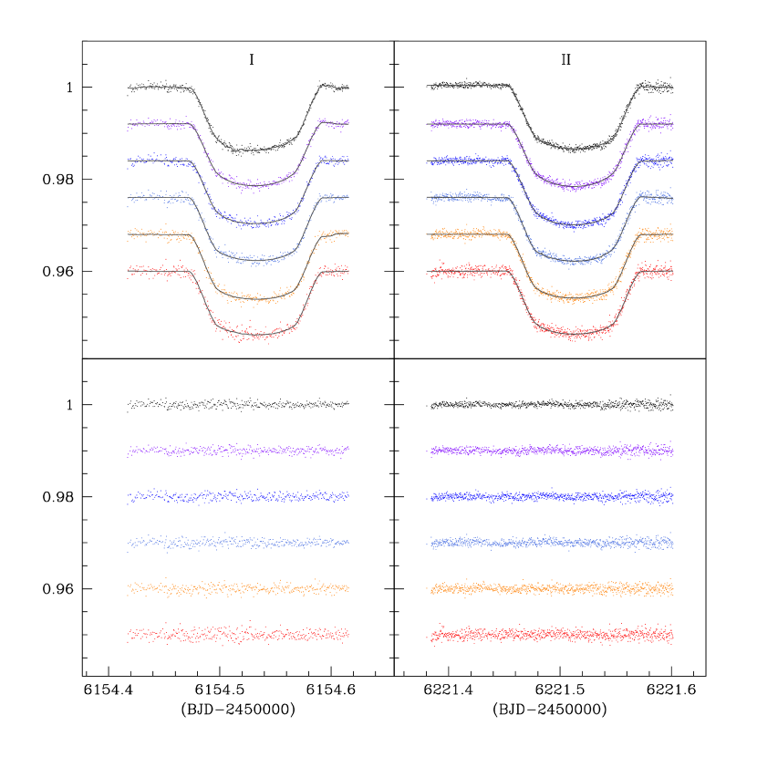
Figure 3: Top panels: lightcurves extracted from the data. The white lightcurve are on top followed by the color lightcurves from the bluest to the reddest one (from top to bottom). An offset is applied for clarity. Bottom panels: Residuals of the fit ordered as in the top panels. Left panels denote results from the first night, right panels from the second.

Table 1: Observations

Date	Epoch	Texp	Airmass range	N. spectra
14/08/2012	487	12	1.9-1.0	350
20/10/2012	502	12	1.0-1.6	809

Table 2: Epochs used in the ephemerides calculation

Epoch	Time of transit minimum (BJD)	Error (BJD)	Reference
0	3979.93071	0.00069	2
1	3984.39780	0.00900	1
2	3988.86274	0.00076	2
4	3997.79277	0.00054	2
4	3997.79425	0.00047	2
6	4006.72403	0.00059	2
8	4015.65410	0.00110	2
20	4069.23870	0.00290	2
86	4363.94677	0.00091	3
90	4381.80920	0.00130	3
469	6074.15737	0.00018	4
470	6078.62307	0.00018	4
478	6114.34537	0.00020	4
487	6154.53253	0.00015	5
495	6190.25542	0.00018	4
502	6221.51261	0.00019	5

Table 3: White lightcurves best fit parameters

$\rm R_{p}/R_{\star}$	T0(days)	T14(days)	$\rm\rho$(g cm-3)	g1	g2	c1	c2	c3	c4
$0.1153_{-0.0011}^{+0.0006}$	$6154.53253_{-0.00013}^{+0.00018}$	$0.11984_{-0.00094}^{+0.00078}$	$0.981_{-0.051}^{+0.057}$	$0.420_{-0.045}^{+0.048}$	$0.2875$	$-0.00024_{-0.00020}^{+0.00010}$	$-0.000047_{-0.000018}^{+0.000015}$	$-0.00114_{-0.00019}^{+0.00017}$	$1.00195_{-0.00037}^{+0.00031}$
$0.11633_{-0.00065}^{+0.00079}$	$6221.51261_{-0.00017}^{+0.00022}$	$0.12007_{-0.00056}^{+0.00062}$	$0.916_{-0.043}^{+0.028}$	$0.393_{-0.045}^{+0.038}$	0.2875	$-0.0008_{-0.0015}^{+0.0002}$	$0.000000_{-0.000016}^{+0.000036}$	$0$	$1.0013_{-0.0005}^{+0.0013}$

Table 4: Spectral band lightcurves best fit parameters

Band ($\rm\AA$)	$\rm R_{p}/R_{\star}$	g1	g2	c1	c2	c3	c4
$4906$-$5600$	$0.11520_{-0.00041}^{+0.00038}$	$0.495_{-0.022}^{+0.014}$	0.2644	$-0.00015_{-0.00022}^{+0.00010}$	$-0.000032_{-0.000015}^{+0.000013}$	$-0.00013_{-0.00022}^{+0.00015}$	$1.00048_{-0.00038}^{+0.00036}$
$5600$-$6183$	$0.11562_{-0.00059}^{+0.00051}$	$0.414_{-0.035}^{+0.019}$	0.2917	$-0.00005_{-0.00027}^{+0.00016}$	$-0.000005_{-0.000022}^{+0.000018}$	$-0.00019_{-0.00028}^{+0.00024}$	$1.00034_{-0.00057}^{+0.00045}$
$6183$-$6780$	$0.11562_{-0.00050}^{+0.00049}$	$0.335_{-0.032}^{+0.021}$	0.3045	$0.00005_{-0.00024}^{+0.00016}$	$0.000005_{-0.000023}^{+0.000014}$	$0.00005_{-0.00025}^{+0.00025}$	$0.99985_{-0.00060}^{+0.00037}$
$6780$-$7390$	$0.11682_{-0.00053}^{+0.00038}$	$0.315_{-0.030}^{+0.019}$	0.2945	$0.00009_{-0.00019}^{+0.00018}$	$0.000057_{-0.000020}^{+0.000015}$	$-0.00010_{-0.00027}^{+0.00021}$	$0.99993_{-0.00057}^{+0.00037}$
$7390$-$7942$	$0.11617_{-0.00056}^{+0.00052}$	$0.302_{-0.034}^{+0.025}$	0.2933	$0.00011_{-0.00026}^{+0.00017}$	$0.000009_{-0.000022}^{+0.000019}$	$0.00022_{-0.00039}^{+0.00021}$	$0.99950_{-0.00057}^{+0.00057}$
$4906$-$5600$	$0.11514_{-0.00038}^{+0.00036}$	$0.519_{-0.017}^{+0.011}$	0.2644	$0.00003_{-0.00064}^{+0.00036}$	$0.000001_{-0.000014}^{+0.000014}$	$0$	$0.99995_{-0.00052}^{+0.00052}$
$5600$-$6183$	$0.11615_{-0.00038}^{+0.00038}$	$0.443_{-0.018}^{+0.011}$	0.2917	$0.00105_{-0.00075}^{+0.00037}$	$-0.000033_{-0.000014}^{+0.000016}$	$0$	$0.99891_{-0.00057}^{+0.00061}$
$6183$-$6780$	$0.11733_{-0.00055}^{+0.00040}$	$0.390_{-0.020}^{+0.017}$	0.3045	$-0.00182_{-0.00077}^{+0.00058}$	$0.000055_{-0.000020}^{+0.000016}$	$0$	$1.00190_{-0.00082}^{+0.00059}$
$6780$-$7390$	$0.11616_{-0.00035}^{+0.00032}$	$0.345_{-0.015}^{+0.014}$	0.2945	$0.00054_{-0.00048}^{+0.00050}$	$-0.000019_{-0.000017}^{+0.000010}$	$0$	$0.99946_{-0.00067}^{+0.00035}$
$7390$-$7942$	$0.11534_{-0.00037}^{+0.00067}$	$0.370_{-0.027}^{+0.014}$	0.2933	$0.0007_{-0.0013}^{+0.0002}$	$-0.000023_{-0.000012}^{+0.000029}$	$0$	$0.9993_{-0.0005}^{+0.0011}$

Table 5: Final radius ratio measurements

Band ($\rm\AA$)	$\rm R_{p}/R_{\star}$	$\rm\sigma(R_{p}/R_{\star})$
$4906$-$5600$	0.1152	0.0003
$5600$-$6183$	0.1160	0.0003
$6183$-$6780$	0.1165	0.0003
$6780$-$7390$	0.1164	0.0003
$7390$-$7942$	0.1157	0.0004

References

- Bakos et al. (2007) Bakos, G. Á., Noyes, R. W., Kovács, G. et al. 2007, ApJ, 656, 552
- Becky et al. (2013) Béky, B., Holman, M. J., Gilliland, R. L. et al. 2013, AJ, 145, 166
- Brown et al. (2001) Brown, T. M. 2001, ApJ, 553, 1006
- Burrows et al. (2007) Burrows, A., Hubeny, I., Budaj, J. et al. 2007, ApJ, 668, 171
- Burrows et al. (2008) Burrows, A. & Budaj, J., Hubeny, I. 2008, ApJ, 678, 1436
- Castelli & Kurucz (2003) Castelli, F., & Kurucz, R. L. 2003, Modelling of Stellar Atmospheres, 210, 20P
- Charbonneau et al. (2002) Charbonneau, D., Brown, T. M., Noyes, R. W. et al. 2002, ApJ, 568, 377
- Claret & Bloemen (2011) Claret, A. & Bloemen, S. 2011, A&A, 529, 75
- Desert et al. (2013) Désert, J., M., Vidal-Madjar, A., Lecavelier Des Etangs, A. et al. 2008, A&A, 492, 585
- Diamond-Lowe et al. (2014) Diamond-Lowe, H., Stevenson, K., B.; Bean, J., L. et al. 2014, ApJ, 796, 66
- Evans et al. (2015) Evans, T. M., Aigrain, S., Gibson, N. et al. 2015, MNRAS, 451, 5199
- Ehrenreich et al. (2006) Ehrenreich, D., Tinetti, G., Lecavelier des Entangs, A. et al. 2006, A&A, 448, 379
- Espinoza & Joran (2015) Espinoza, N. & Jordán 2015, MNRAS, 450, 1879
- Fortney et al. (2006) Fortney, J. J., Cooper, C. S., Showman, A. P. et al. 2006, ApJ, 652, 746
- Fortney et al. (2008) Fortney, J. J., Lodders, K., Marley, M. S. et al. 2008, ApJ, 678, 1419
- Fortney et al. (2010) Fortney, J. J., Shabram, M., Showman, A. P. et al. 2010, ApJ, 709, 1396
- Gilliland et al. (1993) Gilliland, R. L.; Brown, T. M.; Kjeldsen, H. et al. 1993, AJ, 106, 2441
- Hubeny et al. (2003) Hubeny, I.; Burrows, A.; Sudarsky, D. 2003, ApJ, 594, 1011
- Huitson et al. (2013) Huitson, C. M., Sing, D. K., Pont, F. et al. 2013, MNRAS, 434, 3252
- Iro et al. (2005) Iro, N., Bézard, B., & Guillot, T. 2005, A&A, 436, 719
- Iro & Deming (2010) Iro, N., & Deming, L. D. 2010, ApJ, 712, 218
- Jensen et al. (2012) Jensen, A. G., Redfield, S., Endl, M. et al. 2011. ApJ, 743, 203
- Johnson et al. (2008) Johnson, J. A., Winn, J. N.; Narita, N. et al. 2008, ApJ, 686, 649
- Knutson et al. (2010) Knutson, H. A., Howard, A. W.& Isaacson, H. 2010, ApJ, 720, 1569
- Mandel & Agol (2002) Mandel, K., & Agol, E. 2002, ApJ, 580, 171
- Montalto et al. (2012) Montalto, M., Gregorio, J., Boué et al. 2012, MNRAS, 427, 2757
- Nikolov et al. (2014) Nikolov, N., Sing, D. K., Pont, F., et al. 2014, MNRAS, 437, 46
- Oshagh et al. (2014) Oshagh, M., Santos, N. C., Ehrenreich, D. et al. 2014, A&A, 568, 99
- Pál (2008) Pál, A. 2008, MNRAS, 390, 281
- Press (1992) Press, W. H., Cambridge: University Press, —c1992, 2nd ed., Numerical recipes in FORTRAN. The art of scientific computing.
- Pont et al. (2013) Pont, F., Sing, D. K., Gibson, N. P. et al. 2013, MNRAS, 432, 2917
- Redfield et al. (2008) Redfield, S., Endl, M., Cochran, W. D., et al. 2008, ApJ, 673, 87
- Rothman et al. (2009) Rothman, L. S., Gordon, I. E., Barbe, A., et al. 2009, J. Quant. Spec. Radiat. Transf., 110, 533
- Rothman et al. (2010) Rothman, L. S., Gordon, I. E., Barber, R. J., et al. 2010, J. Quant. Spec. Radiat. Transf., 111, 2139
- Santos et al. (2013) Santos, N. C., Sousa, S. G., Mortier, A. et al. 2013, A&A, 556, 150
- Seager (2000) Seager, S. & Sasselov, D. D. 2000, ApJ, 540, 504
- Sing et al. (2011) Sing, D. K., Désert, J.-M., Fortney, J. J., et al. 2011, A&A, 527, 73
- Sing et al. (2013) Sing, D. K., Lecavelier des Etangs, A., Fortney, J. J. et al. 2013, MNRAS, 436, 2956
- Sing et al. (2015) Sing, D. K., Wakeford, H. R., Showman, A. P. 2015, MNRAS, 446, 2428
- Snellen et al. (2008) Snellen, I. A. G., Albrecht, S., de Mooij, E. J. W. et al. 2008, A&A, 487, 357
- Stevenson et al. (2014) Stevenson, K. B., Bean, J. L., Seifahrt, A. et al. 2014, AJ, 147, 161
- Todorov et al. (2010) Todorov, K., Deming, D., Harrington, J. et al. 2010, ApJ, 708, 498
- Young & Irvine (1967) Young, A. T., Irvine, W. M. 1967, AJ, 72, 945
- Wakeford et al. (2013) Wakeford, H. R., Sing, D. K., Deming, D. et al. 2013, MNRAS, 435, 3481
- Wilson et al. (2015) Wilson, P. A., Sing, D. K., Nikolov, N. et al. 2015, MNRAS, 450, 192
- Winn et al. (2007) Winn, J. N., Holman, M. J., Bakos, G. Á. et al. 2007, AJ, 134, 1707
- Wood et al. (2011) Wood, P. L., Maxted, P. F. L., Smalley, B. et al. 2011, MNRAS, 412, 2376
- Zahnle et al. (2009) Zahnle, K., Marley, M. S., Freedman, R. S. et al. 2009, ApJ, 701, 20
- Zhou et al. (2012) Zhou, G. & Bayliss, D. D. R. 2012, MNRAS, 426, 2483