Shift Symmetry and Higgs Inflation in Supergravity with Observable Gravitational Waves

Abstract:

We demonstrate how to realize within supergravity a novel chaotic-type inflationary scenario driven by the radial parts of a conjugate pair of Higgs superfields causing the spontaneous breaking of a grand unified gauge symmetry at a scale assuming the value of the supersymmetric grand unification scale. The superpotential is uniquely determined at the renormalizable level by the gauge symmetry and a continuous $R$ symmetry. We select two types of Kähler potentials, which respect these symmetries as well as an approximate shift symmetry. In particular, they include in a logarithm a dominant shift-symmetric term proportional to a parameter $c_{-}$ together with a small term violating this symmetry and characterized by a parameter $c_{+}$. In both cases, imposing a lower bound on $c_{-}$, inflation can be attained with subplanckian values of the original inflaton, while the corresponding effective theory respects perturbative unitarity for $r_{\pm}=c_{+}/c_{-}\leq 1$. These inflationary models do not lead to overproduction of cosmic defects, are largely independent of the one-loop radiative corrections and accommodate, for natural values of $r_{\pm}$, observable gravitational waves consistently with all the current observational data. The inflaton mass is mostly confined in the range $(3.7-8.1)\times 10^{10}~{}{\mbox{\rm GeV}}$.

Keywords: Cosmology of Theories Beyond the Standard Model, Supergravity Models;
PACS codes: 98.80.Cq, 11.30.Qc, 12.60.Jv, 04.65.+e

Published in J. High Energy Phys. 11, 114 (2015)

1 Introduction

The announcement of the recent joint analysis of the Bicep2/Keck Array and Planck data [1, 2] confirms earlier attempts [3, 4] which stressed the impact of the dust foreground on the observations on the B-mode in the polarization of the cosmic microwave background radiation at large angular scales. As a consequence, the predicted tensor-to-scalar ratio $r$ in inflationary models must be smaller than the one initially claimed in Ref. [5]. However, the present data not only leave open the possibility for a sizable value of $r$, but also seem to favor values of $r$ of order $0.01$. Indeed, it has been reported that

$$r=0.048^{+0.035}_{-0.032}$$ (1)

at 68$\%$ confidence level (c.l.). This fact motivates us to explore the question whether realistic supersymmetric (SUSY) inflation models can accommodate such values of $r$ – for similar attempts see Refs. [6, 7, 8, 9, 10].

One elegant SUSY model which can nicely combine inflation with the Higgs mechanism of the symmetry breaking is the model of Higgs inflation (HI). This is an inflationary model of the chaotic type, where a Higgs field plays the role of inflaton before its trapping in the vacuum. It has been shown that HI in the framework of supergravity (SUGRA) can be implemented by imposing [11, 13, 14, 12, 15] a convenient shift symmetry on the Kähler potential or invoking [17, 18, 16] a logarithmic Kähler potential with a real subdominant kinetic part and a dominant holomorphic (and anti-holomorphic) part, which plays the role of a non-minimal coupling to the Ricci scalar curvature [19, 20]. Inspired by these efforts, we present here a ‘hybrid’ scenario, where a conjugate pair of Higgs superfields is involved in the logarithmic part of the Kähler potential $K$, which respects a shift symmetry with a tiny violation – cf. Refs. [21, 22, 10]. The shift-symmetry-preserving part of $K$ influences the amplitude of the canonically normalized inflaton, which becomes much larger than the original inflaton field appearing in the superpotential and the Kähler potential – cf. Ref. [8]. Therefore, HI can be implemented even with subplanckian values of the original inflaton field, keeping corrections from higher order terms harmless. On the other hand, the resulting inflationary potential does not depend directly on the strength of the shift-symmetry-preserving part of $K$ and, thus, is not flattened drastically as in the original scenario of non-minimal HI [16, 17, 18], but just adequately by the shift-symmetry-violating part of $K$, as in the recently proposed models of kinetically modified non-minimal inflation [10]. Moreover, invoking deviations from the prefactors $-3$ or $-2$ of the logarithms in the proposed Kähler potentials, we succeed to enhance the resulting values of $r$ – cf. Refs. [6, 8, 9]. We also analyze the impact of the one-loop radiative corrections (RCs) [23] on our results and find that these can be kept under control provided that the relevant renormalization scale is conveniently chosen [24]. We, finally, show that the ultraviolet (UV) cut-off scale [25, 26, 27] in these models coincides with the Planck scale and so concerns regarding their naturalness can be safely eluded.

We exemplify our proposal in the context of a grand unified theory (GUT) model based on the gauge group $G_{B-L}=G_{\rm SM}\times U(1)_{B-L}$ – where ${G_{\rm SM}}=SU(3)_{\rm c}\times SU(2)_{\rm L}\times U(1)_{Y}$ is the gauge group of the standard model and $B$ and $L$ denote the baryon and lepton number, respectively. Actually, this is a minimal extension of the minimal supersymmetric standard model (MSSM) which is obtained by promoting the already existing $U(1)_{B-L}$ global symmetry to a local one. As a consequence, the presence of right-handed neutrinos $\nu^{c}_{i}$ is necessary in order to cancel the $B-L$ gauge anomaly. The Higgs fields which cause the spontaneous breaking of the $G_{B-L}$ symmetry to ${G_{\rm SM}}$ can naturally play the role of inflaton. This breaking provides large Majorana masses to the $\nu^{c}_{i}$’s, which then generate the tiny neutrino masses via the seesaw mechanism. Furthermore, the out-of-equilibrium decay of the $\nu^{c}_{i}$’s provides us with a robust baryogenesis scenario via non-thermal leptogenesis [28].

It is worth emphasizing that $U(1)_{B-L}$ is already spontaneously broken during HI through the non-zero values acquired by the relevant Higgs fields. Consequently, HI is not followed by the production of cosmic strings and, therefore, no extra restrictions [29] on the model parameters have to be imposed, in contrast to the case of the standard F-term hybrid inflation (FHI) [30] models, which share the same superpotential with our models. In the standard FHI models, the GUT gauge symmetry is unbroken during inflation since the Higgs superfields are confined to zero and the inflaton is a gauge singlet. The spontaneous breaking of the GUT gauge symmetry takes place at the end of FHI, where the Higgs fields acquire non-zero values. Topological defects are, thus, copiously formed if they are predicted by the symmetry breaking. In our present scheme, this same gauge singlet superfield is stabilized at zero during and after HI. We consider two possible embeddings of the gauge singlet superfield in $K$ with its kinetic terms included or not included in the logarithm together with those of the inflaton.

The superpotential and Kähler potentials of our models are presented in Sec. 2. In Sec. 3, we describe the inflationary potential at tree level and after including the one-loop RCs, whereas, in Sec. 4, we derive the inflationary observables and confront them with observations. We then provide an analysis of the UV behavior of these models in Sec. 5. Our conclusions are summarized in Sec. 6. Throughout the paper, we use units where the reduced Planck scale $m_{\rm P}=2.433\times 10^{18}~{}{\mbox{\rm GeV}}$ is set equal to unity, subscripts of the type $,\chi$ denote derivation with respect to (w.r.t.) the field $\chi$ (e.g. $F_{,\chi\chi}=\partial^{2}F/\partial\chi^{2}$), and charge conjugation is denoted by a star.

2 Modeling Shift Symmetry for Higgs Inflation

We will now explain how a conveniently modified shift symmetry can be used in order to implement HI based on the F-term SUGRA potential. The structure of the superpotential is presented in Sec. 2.1, whereas the relevant Kähler potential is given in Sec. 2.2. Finally, in Sec. 2.3, we derive the corresponding frame function.

2.1 The superpotential

Superfields	$S$	$\Phi$	$\bar{\Phi}$
$U(1)_{B-L}$	$0$	$1$	$-1$
$U(1)_{R}$	$1$	$0$	$0$

Table 1: Charge assignments of the superfields.

We focus on a minimal extension of the MSSM based on the gauge group $G_{B-L}$, which can be broken down to $G_{\rm SM}$ at a scale close to the SUSY GUT scale $M_{\rm GUT}$ through the vacuum expectation values acquired by a conjugate pair of left-handed Higgs superfields $\Phi$ and $\bar{\Phi}$ charged oppositely under $U(1)_{B-L}$ – see Table 1. The part of the superpotential $W$ which is relevant for inflation is given by [30]

$$W=\lambda S\left(\bar{\Phi}\Phi-M^{2}/4\right),$$ (2)

where $S$ is a gauge singlet superfield, $\lambda$ a dimensionless parameter, and $M$ a mass scale of order $M_{\rm GUT}$. This superpotential is the most general renormalizable superpotential which respects an $R$ symmetry $U(1)_{R}$ – see Table 1 – in addition to the aforementioned $G_{B-L}$. The $R$ symmetry guarantees the linearity of the superpotential w.r.t. the gauge singlet superfield $S$. This fact is helpful both for the realization of HI and the determination of the SUSY vacuum.

To verify that $W$ leads to the breaking of $G_{B-L}$ down to $G_{\rm SM}$, we minimize the SUSY limit $V_{\rm SUSY}$ of the SUGRA scalar potential derived from the superpotential in Eq. (2) and the common SUSY limit of the Kähler potentials in Eqs. (9) and (10) – see below. The potential $V_{\rm SUSY}$, which includes contributions from F- and D-terms, turns out to be

$$V_{\rm SUSY}=\lambda^{2}\left|\bar{\Phi}\Phi-\frac{M^{2}}{4}\right|^{2}+\frac{\lambda^{2}}{c_{-}(1-Nr_{\pm})}|S|^{2}\left(|\bar{\Phi}|^{2}+|\Phi|^{2}\right)+\frac{g^{2}}{2}c_{-}^{2}(1-Nr_{\pm})^{2}\left(|\bar{\Phi}|^{2}-|\Phi|^{2}\right)^{2}\,,$$ (3a)

where the complex scalar components of the various superfields are denoted by the same superfield symbol, $$g N,c_{-},r_{\pm} |\bar{\Phi}|=|\Phi|$$ is the unified gauge coupling constant, and the remaining parameters () are defined in Secs. 2.2 and 2.3. From the last equation, we find that the SUSY vacuum lies along the D-flat direction with

$$\langle{S}\rangle=0\>\>\>\mbox{and}\>\>\>|\langle{\Phi}\rangle|=|\langle{\bar{\Phi}}\rangle|=M/2.$$ (3b)

Although $\langle{\Phi}\rangle$ and $\langle{\bar{\Phi}}\rangle$ break spontaneously $U(1)_{B-L}$, no cosmic strings are produced at the end of inflation, since this symmetry is already broken during HI. Needless to say that contributions from the soft SUSY breaking terms can be safely neglected since the corresponding mass scale is much smaller than $M$. Let us emphasize, however, that soft SUSY breaking effects break $U(1)_{R}$ explicitly to a discrete subgroup. Usually, the combination of the latter with the $\mathbb{Z}_{2}^{\rm f}$ fermion parity yields [31] the well-known $R$-parity of MSSM, which guarantees the stability of the lightest SUSY particle and, therefore, provides a well-motivated cold dark matter candidate.

2.2 The Kähler Potential

The superpotential $W$ in Eq. (2) could give rise to HI driven by the real field $\phi$ defined in the standard parametrization

$$\Phi=\frac{\phi}{\sqrt{2}}e^{i{\theta}}\cos{\theta_{\Phi}},\>\>\>\bar{\Phi}=\frac{\phi}{\sqrt{2}}e^{i{\bar{\theta}}}\sin{\theta_{\Phi}}\>\>\>\mbox{with}\>\>\>0\leq{\theta_{\Phi}}\leq\frac{\pi}{2}\>\>\>\mbox{and}\>\>\>S=\frac{s+i\bar{s}}{\sqrt{2}}$$ (4)

provided that we confine ourselves to the field configuration

$$s=\bar{s}={\theta}={\bar{\theta}}=0\>\>\>\mbox{and}\>\>\>{\theta_{\Phi}}={\pi/4}.$$ (5)

Note that the last equality ensures the D-flatness of the potential. Indeed, along this trajectory, $V_{\rm SUSY}$ in Eq. (3a) reduces to the well-known F-term potential which is quartic w.r.t. $\phi$. This construction, though, can become meaningful only if it can be successfully embedded in SUGRA, due to the transplanckian values of $\phi$ which may be needed – see below.

To this end and following similar works [11, 13, 15], we require that the Kähler potential is consistent with the shift symmetry

$$\Phi\ \rightarrow\ \Phi+C,~{}\bar{\Phi}\ \rightarrow\ \bar{\Phi}+C^{*},~{}S\rightarrow\ S$$ (6a)

with $$C$$ being any complex number. Under this symmetry, the real quantities

$$F_{-}=\left|\Phi-\bar{\Phi}^{*}\right|^{2}~{}~{}~{}\mbox{and}~{}~{}~{}F_{S}={|S|^{2}}-{k_{S}}{|S|^{4}}$$ (6b)

are invariant and can, thus, be used in the construction of the Kähler potential. The last term in the right-hand side of the equation for $F_{S}$ with $k_{S}\sim 1$ is included in order to ensure that the mass squared of $S$ during HI is large and positive – see Sec. 3.2. If one combines the superpotential in Eq. (2) with a canonical-like [13] or a logarithmic Kähler potential involving $F_{-}$ and $F_{S}$, one can show that HI driven by the simplest quartic potential with transplanckian values of $\phi$ can be attained. Namely, in Ref. [13], a symmetry similar to the one in Eq. (6a) is conveniently applied in the case of the $SU(2)_{\rm L}$ doublets of MSSM. This model, though, is by now ruled out [2] due to the relatively low value of $n_{\rm s}$ ($n_{\rm s}\simeq 0.947$) and the high value of $r$ ($r\simeq 0.28$) that it predicts – see e.g. Refs. [32, 2].

We are forced, therefore, to allow a tiny violation of the shift symmetry in Eq. (6a) including at the level of the quadratic terms in the Kähler potential a subdominant term of the form

$$F_{+}=\left|\Phi+\bar{\Phi}^{*}\right|^{2},$$ (7)

which remains invariant under the transformation

$$\Phi\ \rightarrow\ \Phi+C,~{}\bar{\Phi}\ \rightarrow\ \bar{\Phi}-C^{*},~{}S\ \rightarrow\ S$$ (8)

coinciding with the one in Eq. (6a) only for $C=0$. Both $F_{-}$ and $F_{+}$ respect the symmetries imposed on $W$ and generate kinetic mixing between $\Phi$ and $\bar{\Phi}$ with non-vanishing eigenvalues. However, positive eigenvalues of the kinetic mixing of $\Phi$ and $\bar{\Phi}$ for a logarithmic Kähler potential are provided by $F_{-}$, which has, thus, to play a prominent role – see Sec. 3.1. The quantity $F_{-}$, contrary to $F_{+}$, vanishes along the trajectory in Eq. (5) and it is expected to contribute only to the normalization of the inflaton field, whereas $F_{+}$ is expected to have an impact on both the normalization of the inflaton and the inflationary potential.

Including the terms in Eqs. (6b) and (7) in a canonical-like Kähler potential, we obtain a model which can become just marginally compatible with the data as mentioned in Ref. [13]. Here, we adopt two other alternatives, i.e. a purely logarithmic Kähler potential

$$K_{1}=-{N_{1}}\ln\left(1-\frac{c_{-}}{{N_{1}}}F_{-}+c_{+}F_{+}-\frac{1}{{N_{1}}}F_{S}+\frac{k_{-}}{{N_{1}}}F_{-}^{2}+\frac{k_{S-}}{{N_{1}}}F_{-}|S|^{2}\right)\,,$$ (9)

or a ‘hybrid’ Kähler potential

$$K_{2}=-{N_{2}}\ln\left(1-\frac{c_{-}}{{N_{2}}}F_{-}+c_{+}F_{+}\right)+F_{S}\,$$ (10)

with one logarithmic term for $\Phi$ and $\bar{\Phi}$ and one canonical-like kinetic term for $S$. In both cases, positivity of the kinetic energy requires ${N_{1}}>0$ and ${N_{2}}>0$. We also introduced two dimensionless coupling constants $c_{-}$ and $c_{+}$ with a clear hierarchy $c_{-}\gg c_{+}$ so that the shift symmetry in Eq. (6a) is the dominant symmetry of the Kähler potential compared to that in Eq. (8). It is worth mentioning that our models are completely natural in the ’t Hooft sense because, in the limit $c_{+}\rightarrow 0$ and $\lambda\rightarrow 0$, the shift symmetry in Eq. (6a) becomes exact and a $U(1)$ symmetry under which $S\rightarrow\ e^{i\alpha}S$ ($\alpha$ is a real number) appears.

Note, finally, that the scenario of non-minimal HI investigated in Refs. [17, 18] can be recovered by doing the substitutions

$$c_{-}=1+Nc_{\cal R}~{}~{}\mbox{and}~{}~{}c_{+}=c_{\cal R}~{}~{}$$ (11)

with $N={N_{1}}=3$ in Eq. (9) or $N={N_{2}}=2$ in Eq. (10) – see below. The symmetries of our model, though, prohibit the existence in the Kähler potential of the terms $|S|^{2}\left(k_{S\Phi}|\Phi|^{2}+k_{S\bar{\Phi}}|\bar{\Phi}|^{2}\right)$ which, generally, violate [32] D-flatness. In this case, the restoration of the D-flatness would require the equality of $k_{S\Phi}$ and $k_{S\bar{\Phi}}$, which signals an ugly tuning of the parameters.

2.3 The Frame Function

The interpretation of the Kähler potentials in Eqs. (9) and (10) can be given in the ‘physical’ Jordan frame (JF). To this end, we derive the JF action for the scalar fields $z^{\alpha}=S,\Phi,\bar{\Phi}$. We start with the corresponding Einstein frame (EF) action within SUGRA [17, 32], which can be written as

$${\sf S}=\int d^{4}x\sqrt{-\widehat{\mathfrak{g}}}\left(-\frac{1}{2}\widehat{\mathcal{R}}+K_{{\alpha}{\bar{\beta}}}\widehat{g}^{\mu\nu}D_{\mu}z^{\alpha}D_{\nu}z^{*{\bar{\beta}}}-\widehat{V}\right),$$ (12a)

where $$\widehat{\mathfrak{g}} \widehat{g}_{\mu\nu} \widehat{\mathcal{R}} D_{\mu} \widehat{V}$$ is the determinant of the EF metric , is the EF Ricci scalar curvature, is the gauge covariant derivative, and is the (tree-level) EF SUGRA scalar potential given by

$$\widehat{V}=\widehat{V}_{\rm F}+\widehat{V}_{\rm D}\>\>\>\mbox{with}\>\>\>\widehat{V}_{\rm F}=e^{K}\left(K^{{\alpha}{\bar{\beta}}}{\rm F}_{\alpha}{\rm F}^{*}_{\bar{\beta}}-3|W|^{2}\right)\>\>\>\mbox{and}\>\>\>\widehat{V}_{\rm D}={1\over 2}g^{2}\sum_{a}{\rm D}_{a}{\rm D}_{a}.$$ (12b)

Here, a trivial gauge kinetic function is adopted and the summation is applied over the generators $$T_{a}$$ of the considered gauge group. Also, we use the shorthand notation

$$K^{{\bar{\beta}}{\alpha}}K_{{\alpha}\bar{\gamma}}=\delta^{\bar{\beta}}_{\bar{\gamma}},\>\>{\rm F}_{\alpha}=W_{,z^{\alpha}}+K_{,z^{\alpha}}W,~{}~{}\mbox{and}~{}~{}{\rm D}_{a}=z^{\alpha}\left(T_{a}\right)_{\alpha}^{\beta}K_{\beta}~{}~{}\mbox{with}~{}~{}K_{{\alpha}}={K_{,z^{\alpha}}},~{}~{}K_{{\alpha}{\bar{\beta}}}={K_{,z^{\alpha}z^{*{\bar{\beta}}}}}.$$ (12c)

If we perform a conformal transformation [17, 32] defining the JF metric $g_{\mu\nu}$ through the relation

$$\widehat{g}_{\mu\nu}=-\frac{\Omega}{N}g_{\mu\nu},\>\>\>\mbox{we obtain}\>\>\>\left\{\begin{matrix}\sqrt{-\widehat{\mathfrak{g}}}={\Omega^{2}\over N^{2}}\sqrt{-\mathfrak{g}},\>\>\>\widehat{g}^{\mu\nu}=-{N\over\Omega}g^{\mu\nu},\hfill\cr\mbox{and}\>\>\>\widehat{\mathcal{R}}=-{N\over\Omega}\left(\mathcal{R}-\Box\ln\Omega+3g^{\mu\nu}\partial_{\mu}\Omega\partial_{\nu}\Omega/2\Omega^{2}\right).\hfill\cr\end{matrix}\right.$$ (13a)

Here $$\Omega \mathfrak{g} g_{\mu\nu} \mathcal{R} N$$ is the frame function, is the determinant of , is the JF Ricci scalar curvature and is a dimensionless parameter which quantifies the deviation from the standard set-up [17]. Upon substitution of Eq. (13a) into Eq. (12a), we end up with the following action in the JF

$${\sf S}=\int d^{4}x\sqrt{-\mathfrak{g}}\left(\frac{\Omega}{2N}\mathcal{R}+\frac{3}{4N\Omega}D_{\mu}\Omega D^{\mu}\Omega-\frac{1}{N}\Omega K_{{\alpha}{{\bar{\beta}}}}D_{\mu}z^{\alpha}D^{\mu}z^{*{\bar{\beta}}}-V\right)\>\>\>\mbox{with}\>\>\>V=\frac{\Omega^{2}}{N^{2}}\widehat{V}\,.$$ (13b)

If, in addition, we connect $\Omega$ to $K$ through the following relation

$$-\Omega/N=e^{-K/N}\>\Rightarrow\>K=-N\ln\left(-\Omega/N\right)$$ (14a)

and take into account the definition [17] of the purely bosonic part of the on-shell value of the auxiliary field

$${\cal A}_{\mu}=i\left(K_{\alpha}D_{\mu}z^{\alpha}-K_{\bar{\alpha}}D_{\mu}z^{*{\bar{\alpha}}}\right)/6,$$ (14b)

we arrive at the following action

$${\sf S}=\int d^{4}x\sqrt{-\mathfrak{g}}\left(\frac{\Omega}{2N}\mathcal{R}+\left(\Omega_{{\alpha}{{\bar{\beta}}}}+\frac{3-N}{N}\frac{\Omega_{{\alpha}}\Omega_{{\bar{\beta}}}}{\Omega}\right)D_{\mu}z^{\alpha}D^{\mu}z^{*{\bar{\beta}}}-\frac{27}{N^{3}}\Omega{\cal A}_{\mu}{\cal A}^{\mu}-V\right),$$ (14c)

where $${\cal A}_{\mu}$$ in Eq. (14b) takes the form

$${\cal A}_{\mu}=-iN\left(\Omega_{\alpha}D_{\mu}z^{\alpha}-\Omega_{\bar{\alpha}}D_{\mu}z^{*{\bar{\alpha}}}\right)/6\Omega\,$$ (14d)

and the shorthand notation $\Omega_{\alpha}=\Omega_{,\Phi^{\alpha}}$ and $\Omega_{\bar{\alpha}}=\Omega_{,\Phi^{*{\bar{\alpha}}}}$ is used. From Eq. (14a), we can find the corresponding frame function during HI as follows

$$f_{\cal R}=-\left.{\Omega\over N}\right|_{\mbox{Eq.~{}(\ref{inftr})}}=\left\{\begin{matrix}(1+c_{+}\phi^{2})^{{N_{1}}/N}\hfill&\mbox{for $K=K_{1}$,}\hfill\cr(1+c_{+}\phi^{2})^{{N_{2}}/N}\hfill\>\>\>&\mbox{for $K=K_{2}$,}\hfill\cr\end{matrix}\right.\,$$ (15)

where we took into account the fact that $F_{-}=F_{S}=0$ along the direction in Eq. (5). Eqs. (14c) and (15) reveal that $f_{\cal R}$ represents the non-minimal coupling to gravity. Note that this function is independent of $c_{-}$, which is to be large for HI with $\phi<1$ – see below. Selecting

$$N={N_{1}}~{}~{}\mbox{or}~{}~{}N={N_{2}}~{}~{}\mbox{for}~{}~{}K={K_{1}}~{}~{}\mbox{or}~{}~{}K={K_{2}}$$ (16)

respectively, we can obtain the standard quadratic non-minimal coupling function. As for the conventional case [17, 18] with one logarithm and $N=3$, when the dynamics of the fields $z^{\alpha}$ is dominated only by the real moduli $|z^{\alpha}|$ or when $z^{\alpha}=0$ for ${\alpha}\neq 1$ [17], we obtain ${\cal A}_{\mu}=0$ in Eq. (14d). The only difference w.r.t. the aforementioned conventional case is that now the scalar fields $z^{\alpha}$ have non-canonical kinetic terms in the JF due to the term proportional to $\Omega_{\alpha}\Omega_{\bar{\beta}}\neq\delta_{{\alpha}{\bar{\beta}}}$. This fact does not cause any problem, since the canonical normalization of the inflaton retains its strong dependence on $c_{-}$ through $\Omega$, whereas the non-inflaton fields become heavy enough during inflation and so they do not affect the dynamics – see Sec. 3.1. Furthermore, for $M\ll m_{\rm P}$, the conventional Einstein gravity at the SUSY vacuum – in Eq. (3b) – is recovered since

$$-\langle{\Omega}\rangle/N\simeq 1.$$ (17)

Given that the analysis of inflation in both the EF and JF yields equivalent results [19], we carry out the derivation of the inflationary observables exclusively in the EF – see Secs. 3.1 and 3.2.

3 The Inflationary Set-up

In this section, we outline the salient features of our inflationary scenario (Sec. 3.1) and then present the one-loop corrected inflationary potential in Sec. 3.2.

3.1 The Tree-level Inflationary Potential

The linearity of $W$ w.r.t. $S$ allows us to isolate easily the non-vanishing contribution of the inflaton to $\widehat{V}_{\rm F}$ on the inflationary path and avoid the runaway behavior which may be caused by the term $-3|W|^{2}\exp{K}$. Indeed, inserting Eqs. (2) and (9) or (10) into Eq. (12b), we find that the only surviving contribution to $\widehat{V}$ on the path in Eq. (5) is

$$\widehat{V}_{\rm HI0}=e^{K}K^{SS^{*}}\,|W_{,S}|^{2}=\frac{\lambda^{2}(\phi^{2}-M^{2})^{2}}{16}\times\left\{\begin{matrix}f_{\cal R}^{-{N_{1}}+1}\hfill&\mbox{for $K=K_{1}$}\hfill\cr f_{\cal R}^{-{N_{2}}}\hfill\>\>\>&\mbox{for $K=K_{2}$.}\hfill\cr\end{matrix}\right.$$ (18)

Here we took into account Eqs. (15) and (16) and the fact that $e^{K}=f_{\cal R}^{-N}$ and $K^{SS^{*}}=f_{\cal R}$ or $K^{SS^{*}}=1$ for $K=K_{1}$ or $K_{2}$ respectively – note that $K_{Sz^{\alpha}}=0$ for both cases and ${\alpha}=2$ or $3$. Introducing a new variable $n$ related to the exponents of $f_{\cal R}$ in Eq. (18), we can cast $\widehat{V}_{\rm HI0}$ in the same form for both the $K$’s in Eqs. (9) and (10). Indeed, $\widehat{V}_{\rm HI0}$ can be rewritten as

$$\widehat{V}_{\rm HI0}=\frac{\lambda^{2}(\phi^{2}-M^{2})^{2}}{16f_{\cal R}^{2(1+n)}},\>\>\mbox{where}\>\>\left\{\begin{matrix}{N_{1}}-1=2(1+n)\hfill\cr{N_{2}}=2(1+n)\hfill\cr\end{matrix}\right.\>\>\mbox{for}\>\>\left\{\begin{matrix}K=K_{1}\hfill\cr K=K_{2}.\hfill\cr\end{matrix}\right.$$ (19)

As anticipated below Eq. (8), $\widehat{V}_{\rm HI0}$ depends exclusively on $c_{+}$ (and not on $c_{-}$). Given that, during HI, $\phi\gg M$ and $c_{+}\phi^{2}>1$ – see below –, $\widehat{V}_{\rm HI0}$ and the corresponding Hubble parameter $\widehat{H}_{\rm HI}$ take the form

$$\widehat{V}_{\rm HI0}\simeq\frac{\lambda^{2}\phi^{-4n}}{16c_{+}^{2(1+n)}}\,\>\>\mbox{and}\>\>\>\widehat{H}_{\rm HI}={\widehat{V}_{\rm HI0}^{1/2}\over\sqrt{3}}\simeq{\lambda\phi^{-2n}\over 4\sqrt{3}c_{+}^{1+n}}\cdot$$ (20)

As a consequence, we obtain an inflationary plateau for $n=0$ or a bounded from below chaotic-type inflationary potential for $n<0$ with $\phi$ in Eq. (4) being a natural inflaton candidate. Note that, thanks to the shift symmetry in Eq. (6a), no mixing term proportional to $k_{S-}$ arises in $\widehat{V}_{\rm HI0}$ in sharp contrast with the models of Refs. [8, 9], where a similar term ($\propto k_{S\Phi}$) plays a crucial role in achieving large values of $r$ in a manner compatible with all observations – see Sec. 4.1.

To specify further our inflationary scenario, we have to determine the EF canonically normalized fields involved. Note that, along the configuration in Eq. (5), the Kähler metric $K_{{\alpha}{\bar{\beta}}}$ defined in Eq. (12c) takes, for both choices of $K$ in Eqs. (9) and (10), the form

$$\left(K_{{\alpha}{\bar{\beta}}}\right)={\sf diag}\left(M_{K},K_{SS^{*}}\right),~{}~{}\mbox{where}~{}~{}M_{K}=\frac{1}{f_{\cal R}^{2}}\mbox{ $\left\lgroup\begin{matrix}\kappa&\bar{\kappa}\cr\bar{\kappa}&\kappa\end{matrix}\right\rgroup$}~{}~{}\mbox{with}~{}~{}\kappa=c_{-}f_{\cal R}-Nc_{+},~{}~{}\bar{\kappa}={Nc_{+}^{2}\phi^{2}},$$ (21)

and $N$ defined in Eq. (16). Given that $K_{SS^{*}}=1/f_{\cal R}$ or $1$ for $K=K_{1}$ or $K_{2}$ respectively, the canonically normalized components $\widehat{s},\widehat{\bar{s}}$ of $S$ – see Eq. (4) – are defined as follows:

$$(\widehat{s},\widehat{\bar{s}})=\sqrt{K_{SS^{*}}}(s,\bar{s}).$$ (22)

The matrix $M_{K}$ can be diagonalized via a similarity transformation involving an orthogonal matrix $U_{K}$ as follows:

$$U_{K}M_{K}U_{K}^{\mbox{\sf\scriptsize T}}={\sf diag}\left(\kappa_{+},\kappa_{-}\right),\>\>\>\mbox{where}\>\>\>U_{K}={1\over\sqrt{2}}\mbox{ $\left\lgroup\begin{matrix}1&1\cr-1&1\end{matrix}\right\rgroup$}$$ (23)

and the eigenvalues of $M_{K}$ are found to be

$$\kappa_{+}=\frac{c_{-}(1-Nr_{\pm})+c_{+}c_{-}(1+Nr_{\pm})\phi^{2}}{f_{\cal R}^{2}}\simeq\frac{c_{-}}{f_{\cal R}}\>\>\>\mbox{and}\>\>\>\kappa_{-}=\frac{c_{-}(1-Nr_{\pm})}{f_{\cal R}}\simeq\frac{c_{-}}{f_{\cal R}},$$ (24)

where the approximate results hold for $r_{\pm}\ll 1/N$ and positivity of $\kappa_{-}$ can be assured only if

$$r_{\pm}<1/N~{}~{}~{}\mbox{with}~{}~{}~{}r_{\pm}=c_{+}/c_{-},$$ (25)

i.e. if $c_{-}>Nc_{+}$, as we anticipated below Eq. (8). This fact has to be contrasted with the original scenario of non-minimal HI [17, 18], where such a constraint is not necessary – as can be verified by inserting Eq. (11) into Eq. (24). In our present cases, the kinetic terms for $z^{\alpha}=\bar{\Phi},\Phi$ can be brought into the following form

$$K_{{\alpha}{\bar{\beta}}}\dot{z}^{\alpha}\dot{z}^{*{\bar{\beta}}}={\kappa_{+}\over 2}\left(\dot{}\phi^{2}+{1\over 2}\phi^{2}\dot{\theta}^{2}_{+}\right)+{\kappa_{-}\phi^{2}\over 2}\left({1\over 2}\dot{\theta}^{2}_{-}+\dot{\theta}^{2}_{\Phi}\right)=\frac{1}{2}\left(\dot{\widehat{}\phi}^{2}+\dot{\widehat{\theta}}_{+}^{2}+\dot{\widehat{\theta}}_{-}^{2}+\dot{\widehat{\theta}}_{\Phi}^{2}\right),$$ (26a)

where $${\theta}_{\pm}=\left(\bar{\theta}\pm{\theta}\right)/\sqrt{2} t$$ and the dot denotes derivation w.r.t. the cosmic time . In the last step, we introduce the EF canonically normalized fields, which are denoted by hat and can be obtained as follows:

$$\frac{d\widehat{\phi}}{d\phi}=J=\sqrt{\kappa_{+}},\>\>\widehat{\theta}_{+}={J\phi\theta_{+}\over\sqrt{2}},\>\>\widehat{\theta}_{-}=\sqrt{\frac{\kappa_{-}}{2}}\phi\theta_{-},\>\>\>\mbox{and}\>\>\>\widehat{\theta}_{\Phi}=\phi\sqrt{\kappa_{-}}\left(\theta_{\Phi}-{\pi\over 4}\right)\cdot$$ (26b)

Note, in passing, that the spinors $\psi_{S}$ and $\psi_{\Phi\pm}$ associated with the superfields $S$ and $\Phi_{\pm}=(\Phi\pm\bar{\Phi})/\sqrt{2}$ are normalized similarly, i.e. $\widehat{\psi}_{S}=\sqrt{K_{SS^{*}}}\psi_{S}$ and $\widehat{\psi}_{\Phi\pm}=\sqrt{\kappa_{\pm}}\psi_{\Phi\pm}$. Integrating the first equation in Eq. (26b), we can express the canonically normalized EF real field $\widehat{\phi}$ as follows:

$$\widehat{\phi}=\widehat{\phi}_{\rm c}+\frac{1}{\sqrt{r_{\pm}}}{\rm arcsinh}\sqrt{c_{+}}\phi$$ (27)

with $\widehat{\phi}_{\rm c}$ being a constant of integration, which we take equal to zero. Note that $\widehat{\phi}$ is practically independent of $N$ (and $n$) – see Eq. (24). Solving Eq. (27) w.r.t. $\phi$, we can express $\widehat{V}_{\rm HI0}$ in Eq. (20) in terms of $\widehat{\phi}$ as follows:

$$\widehat{V}_{\rm HI0}\simeq\frac{\lambda^{2}}{4c_{+}^{2}}\frac{\tanh^{4}\sqrt{r_{\pm}}\widehat{\phi}}{\cosh^{4n}\sqrt{r_{\pm}}\widehat{\phi}}\,\cdot$$ (28)

For $n=0$ and $\lambda=c_{+}=1$, $\widehat{V}_{\rm HI0}$ coincides with the potential encountered in the so-called $T$-models [6] arising from the spontaneous breaking of (super)conformal invariance. We observe that, although $f_{\cal R}$ in Eq. (15) and $\widehat{V}_{\rm HI0}$ in Eq. (28) are independent of $c_{-}$, $\widehat{\phi}$ depends heavily on $c_{-}$ and, therefore, it can be much larger than $\phi$ facilitating the attainment of HI with subplanckian values of $\phi$. As a consequence, the initial fields $\Phi$ and $\bar{\Phi}$ – see Eq. (4) –, which are closely related with $\phi$, can remain also subplanckian, as required for a meaningful approach to SUGRA.

3.2 Stability and One-loop Radiative Corrections

To ensure the validity of our inflationary proposal, we have to check the stability of the direction in Eq. (5) w.r.t. the fluctuations of the fields which are orthogonal to this direction, i.e. we have to examine the fulfillment of the following conditions:

$$\left.{\partial\widehat{V}\over\partial\widehat{\chi}^{\alpha}}\right|_{\mbox{Eq.~{}(\ref{inftr})}}=0\>\>\>\mbox{and}\>\>\>\widehat{m}^{2}_{\chi^{\alpha}}>0\>\>\>\mbox{with}\>\>\>\chi^{\alpha}={\theta_{-}},{\theta_{+}},{\theta_{\Phi}},s,\bar{s}.$$ (29a)

Here $$\widehat{m}^{2}_{\chi^{\alpha}}$$ are the eigenvalues of the mass-squared matrix with elements

$$\widehat{M}^{2}_{{\alpha}{\beta}}=\left.{\partial^{2}\widehat{V}\over\partial\widehat{\chi}^{\alpha}\partial\widehat{\chi}^{\beta}}\right|_{\mbox{Eq.~{}(\ref{inftr})}}\mbox{with}~{}~{}\chi^{\alpha}={\theta_{-}},{\theta_{+}},{\theta_{\Phi}},s,\bar{s}.$$ (29b)

Diagonalizing $\widehat{M}^{2}_{{\alpha}{\beta}}$, we construct the scalar mass-squared spectrum of the theory along the direction in Eq. (5). In Table 2, we present approximate expressions of the relevant masses squared, which are quite close to the rather lengthy exact expressions. Note, however, that our numerical computation uses the exact expressions. In this table, we also include the mass squared $\widehat{m}_{\phi}^{2}$ of $\widehat{\phi}$ as well as the masses squared of the chiral fermions, the gauge boson $A_{BL}$, and the gaugino $\lambda_{BL}$ which are used in our analysis below.

From the formulas displayed in Table 2, we can infer that the stability of the path in Eq. (5) is assured since Eq. (29a) is fulfilled. In particular, it is evident that $k_{S}\gtrsim 1$ assists us to achieve $\widehat{m}^{2}_{{s}}>0$ for $K={K_{1}}$ – in accordance with the results for similar models in Refs. [17, 8]. On the other hand, for $K={K_{2}}$, $\widehat{m}^{2}_{{s}}>0$ even with $k_{S}=0$. However, since there is no observational hint [2] for large non-Gaussianity in the cosmic microwave background, we should make sure that all the $\widehat{m}^{2}_{\chi^{\alpha}}$’s for the scalar fields in Table 2 except $\widehat{m}^{2}_{\phi}$ are greater than $\widehat{H}_{\rm HI}^{2}$ during the last $50-60$ e-foldings of HI. This guarantees that the observed curvature perturbation is generated wholly by $\phi$ as assumed in Eq. (34) – see below. Requiring that $\widehat{m}^{2}_{s}\gg\widehat{H}_{\rm HI}^{2}$ entails the existence of a non-vanishing $k_{S}$ for $K={K_{2}}$ too. Due to the large effective masses that the scalars acquire during HI, they enter a phase of damped oscillations about zero. As a consequence, the $\phi$ dependence in their normalization – see Eq. (26b) – does not affect their dynamics.

Fields	Eigenstates	Masses Squared
			$K=K_{1}$	$K=K_{2}$
3 real scalars	$\widehat{\phi}$	$\widehat{m}^{2}_{\phi}$	$\widehat{\eta}\widehat{H}_{\rm HI}^{2}$
	$\widehat{\theta}_{+}$	$\widehat{m}_{\theta+}^{2}$	$6(1-1/{N_{1}})\widehat{H}_{\rm HI}^{2}$	$6\widehat{H}_{\rm HI}^{2}$
	$\widehat{\theta}_{\Phi}$	$\widehat{m}_{\theta_{\Phi}}^{2}$	$M^{2}_{BL}+6\left(1-\frac{1}{{N_{1}}}\right)\widehat{H}_{\rm HI}^{2}$	$M^{2}_{BL}+6\widehat{H}_{\rm HI}^{2}$
1 complex scalar	$\widehat{s},\widehat{\bar{s}}$	$\widehat{m}_{s}^{2}$	$6\left(2k_{S}f_{\cal R}-\frac{1}{{N_{1}}}\right)\widehat{H}_{\rm HI}^{2}$	$12k_{S}\widehat{H}_{\rm HI}^{2}$
1 gauge boson	$A_{BL}$	$M_{BL}^{2}$	$g^{2}c_{-}(1-Nr_{\pm})\phi^{2}/f_{\cal R}$
$4$ Weyl spinors	$\widehat{\psi}_{\pm}={\widehat{\psi}_{\Phi+}\pm\widehat{\psi}_{S}\over\sqrt{2}}$	$\widehat{m}^{2}_{\psi\pm}$	${6(2+c_{+}(3-{N_{1}})\phi^{2})^{2}\over c_{-}^{2}\phi^{2}f_{\cal R}}\widehat{H}_{\rm HI}^{2}$	${6(2+c_{+}(2-{N_{2}})\phi^{2})^{2}\over c_{-}^{2}\phi^{2}f_{\cal R}}\widehat{H}_{\rm HI}^{2}$
	$\uplambda_{BL},\widehat{\psi}_{\Phi-}$	$M_{BL}^{2}$	$g^{2}c_{-}(1-Nr_{\pm})\phi^{2}/f_{\cal R}$

Table 2: The mass-squared spectrum for $K=K_{1}$ and $K=K_{2}$ along the inflationary trajectory in Eq. (5) for $\phi\ll 1$. $N$ is defined in Eq. (16) and $\widehat{\eta}$ is given by Eq. (40) – see below. To avoid very lengthy formulas, we neglect terms proportional to $M\ll\phi$.

Considering SUGRA as an effective theory below $m_{\rm P}$ allows us to use the well-known Coleman-Weinberg formula [23] in order to find the one-loop corrected inflationary potential

$$\widehat{V}_{\rm HI}=\widehat{V}_{\rm HI0}+\Delta\widehat{V}_{\rm HI}\>\>\>\mbox{with}\>\>\>\Delta\widehat{V}_{\rm HI}=\frac{1}{64\pi^{2}}\sum_{i}(-)^{{\rm F}_{i}}\widehat{m}_{i}^{4}\ln\frac{\widehat{m}_{i}^{2}}{\Lambda^{2}}\,,$$ (30a)

where the sum extends over all helicity states $$i {\rm F}_{i} \widehat{m}_{i}^{2} i \Lambda \widehat{m}_{i}^{2}$$ of the fields listed in Table 2, is the fermion number and the mass squared of the th helicity state, and is a renormalization mass scale. The consistent application of this formula requires that the ’s which enter into the sum are:

• Positive. As a consequence and following the common practice [9, 8, 20], we neglect the contribution of $\widehat{m}_{\phi}^{2}$ to $\Delta\widehat{V}_{\rm HI}$ since this mass squared turns out to be negative in the largest part of the parameter space of our models. Let us recall here that Eq. (30a) is valid only for a static configuration and is uniquely defined only in the extremum points. The proper calculation should use the time-dependent background – see e.g. Ref. [33]. For the non-minimal inflation, this is not done up to now, but we do not expect to get a very unexpected effect if the full computation is consistently carried out.

• Much lighter than a momentum cut-off squared, which is here considered as large as $m_{\rm P}^{2}$. As a consequence, we do not take into account the contributions from $M_{BL}^{2}$ and $\widehat{m}_{\theta_{\Phi}}^{2}$ to $\Delta\widehat{V}_{\rm HI}$ since these masses squared are much larger than $m_{\rm P}^{2}$ in our case given that $c_{-}\gg 1$ – see below. This stems from the form of $\kappa_{-}$ in Eq. (24) and does not occur in the case of the standard non-minimal HI [20, 18], as can be checked by substituting Eq. (11) into the expressions for these masses squared in Table 2.

Having in mind the above subtleties and neglecting contributions from the gravitational sector of the theory, the one-loop RCs read

$$\Delta\widehat{V}_{\rm HI}={1\over 64\pi^{2}}\left(\widehat{m}_{{\theta}_{+}}^{4}\ln{\widehat{m}_{{\theta}_{+}}^{2}\over\Lambda^{2}}+2\widehat{m}_{s}^{4}\ln{m_{\widehat{s}}^{2}\over\Lambda^{2}}-4\widehat{m}_{\psi_{+}}^{4}\ln{\widehat{m}_{\psi_{+}}^{2}\over\Lambda^{2}}\right)\,.$$ (30b)

The renormalization scale $\Lambda$ can be determined by requiring [24] that $\Delta\widehat{V}_{\rm HI}(\phi_{\star})=0$ or $\Delta\widehat{V}_{\rm HI}(\phi_{\rm f})=0$.

Let us, finally, stress here that the non-vanishing value of $\phi$ during HI breaks spontaneously $U(1)_{B-L}$ leading to a Goldstone boson ${\theta}_{-}$. This is ‘eaten’ by the gauge boson $A_{BL}$, which then becomes massive. As a consequence, six degrees of freedom before the spontaneous breaking (four corresponding to the two complex scalars $\Phi$ and $\bar{\Phi}$ and two corresponding to the massless gauge boson $A_{BL}$ of $U(1)_{B-L}$) are redistributed as follows: three degrees of freedom are associated with the real propagating scalars ($\widehat{\phi},\widehat{\theta}_{+}$, and $\widehat{\theta}_{\Phi}$), whereas the residual one degree of freedom combines together with the two ones of the initially massless gauge boson $A_{BL}$ to make it massive. From Table 2, we can deduce that the numbers of bosonic (eight) and fermionic (eight) degrees of freedom are equal, as they should.

4 Constraining the Parameters of the Models

We will now outline the predictions of our inflationary scenarios in Sec. 4.2 and confront them with a number of criteria introduced in Sec. 4.1.

4.1 Inflationary Observables – Constraints

Our inflationary settings can be characterized as successful if they can be compatible with a number of observational and theoretical requirements, which are enumerated in the following – cf. Ref. [34]:

4.1.1.

The number of e-foldings

$$\widehat{N}_{\star}=\int_{\widehat{\phi}_{\rm f}}^{\widehat{\phi}_{\star}}\,d\widehat{\phi}\>\frac{\widehat{V}_{\rm HI}}{\widehat{V}_{\rm HI,\widehat{\phi}}}=\int_{\phi_{\rm f}}^{\phi_{\star}}\,J^{2}\frac{\widehat{V}_{\rm HI}}{\widehat{V}_{\rm HI,\phi}}d\phi$$ (31)

that the pivot scale $k_{\star}=0.05/{\rm Mpc}$ suffers during HI has to take a certain value to resolve the horizon and flatness problems of standard hot big bang cosmology. This requires [2] that

$$\widehat{N}_{\star}\simeq 61.5+\ln{\widehat{V}_{\rm HI}(\phi_{\star})^{1/2}\over\widehat{V}_{\rm HI}(\phi_{\rm f})^{1/4}}+\frac{1-3w_{\rm rh}}{12(1+w_{\rm rh})}\ln\frac{\pi^{2}g_{\rm rh*}T_{\rm rh}^{4}}{30\widehat{V}_{\rm HI}(\phi_{\rm f})}-\frac{1}{12}\ln g_{\rm rh*},$$ (32)

where we assumed that HI is followed, in turn, by a phase of damped inflaton oscillations with mean equation-of-state parameter $w_{\rm rh}$, a radiation dominated era, and a matter dominated period. Here, $T_{\rm rh}$ is the reheat temperature after HI, $g_{\rm rh*}$ is the energy-density effective number of degrees of freedom at $T_{\rm rh}$ – for the MSSM spectrum, we take $g_{\rm rh*}=228.75$ –, $\phi_{\star}~{}[\widehat{\phi}_{\star}]$ is the value of $\phi~{}[\widehat{\phi}]$ when $k_{\star}$ crosses outside the inflationary horizon, and $\phi_{\rm f}~{}[\widehat{\phi}_{\rm f}]$ is the value of $\phi~{}[\widehat{\phi}]$ at the end of HI, which can be found, in the slow-roll approximation, from the condition

$${\sf max}\{\widehat{\epsilon}(\phi_{\rm f}),|\widehat{\eta}(\phi_{\rm f})|\}=1$$ (33a)

with the slow-roll parameters calculated as follows:

$$\widehat{\epsilon}={1\over 2}\left(\frac{\widehat{V}_{\rm HI,\widehat{\phi}}}{\widehat{V}_{\rm HI}}\right)^{2}={1\over 2J^{2}}\left(\frac{\widehat{V}_{\rm HI,\phi}}{\widehat{V}_{\rm HI}}\right)^{2}\>\>\>\mbox{and}\>\>\>\>\>\widehat{\eta}=\frac{\widehat{V}_{\rm HI,\widehat{\phi}\widehat{\phi}}}{\widehat{V}_{\rm HI}}={1\over J^{2}}\left(\frac{\widehat{V}_{\rm HI,\phi\phi}}{\widehat{V}_{\rm HI}}-\frac{\widehat{V}_{\rm HI,\phi}}{\widehat{V}_{\rm HI}}{J_{,\phi}\over J}\right)\cdot$$ (33b)

Given that, for a power-law potential $\phi^{n}$, we have [35, 34] $w_{\rm rh}=(n-2)/(n+2)$, we take for our numerics $w_{\rm rh}=1/3$, which corresponds precisely to $n=4$. Although we expect that, in the our cases, $w_{\rm rh}$ will deviate slightly from this value, we consider this value quite reliable since, for low values of $\phi$, our inflationary potentials can be well approximated by a quartic potential. As a consequence, our set-up is largely independent from $T_{\rm rh}$ – see Eq. (32).

4.1.2.

The amplitude $A_{\rm s}$ of the power spectrum of the curvature perturbation generated by $\phi$ at the pivot scale $k_{\star}$ must be consistent with the data [2]:

$$A_{\rm s}^{1/2}=\>\frac{1}{2\sqrt{3}\,\pi}\;\frac{\widehat{V}_{\rm HI}(\widehat{\phi}_{\star})^{3/2}}{|\widehat{V}_{\rm HI,\widehat{\phi}}(\widehat{\phi}_{\star})|}=\frac{|J(\phi_{\star})|}{2\sqrt{3}\,\pi}\;\frac{\widehat{V}_{\rm HI}(\phi_{\star})^{3/2}}{|\widehat{V}_{\rm HI,\phi}(\phi_{\star})|}\simeq 4.627\times 10^{-5},$$ (34)

where we assume that no other contributions to the observed curvature perturbation exist.

4.1.3.

The remaining inflationary observables, i.e. the scalar spectral index $n_{\rm s}$, its running $a_{\rm s}$, and the tensor-to-scalar ratio $r$, which are given by

$$\mbox{\footnotesize\sf(a)}\>\>\>n_{\rm s}=\>1-6\widehat{\epsilon}_{\star}\ +\ 2\widehat{\eta}_{\star},\>\>\>\mbox{\footnotesize\sf(b)}\>\>\>a_{\rm s}=\>\frac{2}{3}\left(4\widehat{\eta}_{\star}^{2}-(n_{\rm s}-1)^{2}\right)-2\widehat{\xi}_{\star},\>\>\>\mbox{and}\>\>\>\mbox{\footnotesize\sf(c)}\>\>\>r=16\widehat{\epsilon}_{\star},$$ (35)

where

$$\widehat{\xi}=\frac{\widehat{V}_{\rm HI,\widehat{}\phi}\widehat{V}_{\rm HI,\widehat{}\phi\widehat{}\phi\widehat{}\phi}}{\widehat{V}_{\rm HI}^{2}}=\frac{\widehat{V}_{\rm HI,\phi}\,\widehat{\eta}_{,\phi}}{\widehat{V}_{\rm HI}\,J^{2}}+2\widehat{\eta}\widehat{\epsilon}$$ (36)

and the variables with subscript $\star$ are evaluated at $\phi=\phi_{\star}$, must be in agreement with the fitting of the data [2] with the $\Lambda$CDM$+r$ model, i.e.

$$\mbox{\footnotesize\sf(a)}\>\>n_{\rm s}=0.968\pm 0.009~{}~{}~{}\mbox{and}~{}~{}~{}\mbox{\footnotesize\sf(b)}\>\>r\leq 0.12,$$ (37)

at 95$\%$ c.l. with $|a_{\rm s}|\ll 0.01$. Although compatible with Eq. (37b), the present combined Planck and Bicep2/Keck Array results [1] seem to favor models with values of $r$ of order $0.01$ – see Eq. (1).

4.1.4.

To avoid corrections from quantum gravity and any destabilization of our inflationary scenario due to higher order non-renormalizable terms, we impose two additional theoretical constraints on our models – keeping in mind that $\widehat{V}_{\rm HI}(\phi_{\rm f})\leq\widehat{V}_{\rm HI}(\phi_{\star})$:

$$\mbox{\footnotesize\sf(a)}\>\>\widehat{V}_{\rm HI}(\phi_{\star})^{1/4}\leq 1\>\>\>\mbox{and}\>\>\>\mbox{\footnotesize\sf(b)}\>\>\phi_{\star}\leq 1.$$ (38)

As we will show in Sec. 5, the UV cutoff of our model is equal to unity (in units of $m_{\rm P}$) for $r_{\pm}\leq 1$ and so no concerns regarding the validity of the effective theory arise.

4.1.5

The $U(1)_{B-L}$ gauge symmetry does not generate any extra contribution to the renormalization group running of the MSSM gauge coupling constants and so the scale $M$ and the relevant gauge coupling constant $g_{B-L}$ can be much lower than the values dictated by the unification of the gauge coupling constants within the MSSM. However, for definiteness, we consider here the most predictive case in which $g_{B-L}=g$ ($g\simeq 0.7$ is the SUSY GUT gauge coupling constant) and $M$ is determined by requiring that $\langle{\Phi}\rangle$ and $\langle{\bar{\Phi}}\rangle$ take values compatible with the unification of the MSSM gauge coupling constants. In particular, the SUSY GUT scale $M_{\rm GUT}\simeq(2/2.433)\times 10^{-2}$ is to be identified with the lowest mass scale of the model at the SUSY vacuum in Eq. (3b), i.e.

$${\sqrt{c_{-}(1-Nr_{\pm})}gM\over\sqrt{f_{\cal R}(\phi=M)}}=M_{\rm GUT}\>\Rightarrow\>M=\frac{M_{\rm GUT}}{\sqrt{g^{2}c_{-}(1-Nr_{\pm})-c_{+}M_{\rm GUT}^{2}}}\simeq\frac{M_{\rm GUT}}{g\sqrt{c_{-}}}.$$ (39)

The requirement that the expression $g^{2}c_{-}(1-Nr_{\pm})-c_{+}M_{\rm GUT}^{2}$ is positive sets an upper bound on $c_{+}$ for every $c_{-}$. Namely, we should have $c_{+}\leq g^{2}(1-Nr_{\pm})c_{-}/M_{\rm GUT}^{2}$, which, however, is too loose to restrict the parameters.

4.2 Analytic Results

Our analytic results are based on the tree-level inflationary potential in Eq. (19) and are identical for both $K={K_{1}}$ and $K={K_{2}}$ provided that ${N_{1}}$ and ${N_{2}}$ are related to $n$ as shown in this equation. Note that, not only the form of $\widehat{V}_{\rm HI0}$ in Eq. (19), but also the canonical normalization of $\phi$ is practically identical in the two cases – see Eqs. (24) and (26b). The slow-roll parameters read

$$\widehat{\epsilon}=\frac{8(1-nc_{+}\phi^{2})^{2}}{c_{-}\phi^{2}f_{\cal R}}\>\>\>\mbox{and}\>\>\>\widehat{\eta}=4\frac{3+c_{+}\phi^{2}\left(n\left(4nc_{+}\phi^{2}-9\right)-2\right)}{c_{-}\phi^{2}f_{\cal R}}\cdot$$ (40)

The termination of HI is triggered by the violation of the $\widehat{\eta}$ criterion at a value of $\phi$ equal to $\phi_{\rm f}$. Since $\phi_{\rm f}\ll\phi_{\star}$, the slow-roll parameters in Eq. (40) can be well approximated by performing an expansion for small values of $\phi$. We find

$$\widehat{\epsilon}\simeq 8\frac{1-(1+2n)c_{+}\phi^{2}}{c_{-}\phi^{2}}~{}~{}~{}\mbox{and}~{}~{}~{}\widehat{\eta}\simeq 4\frac{3-(5+9n)c_{+}\phi^{2}}{c_{-}\phi^{2}}\,\cdot$$ (41)

Employing these expressions, $\phi_{\rm f}$ is calculated to be

$$\widehat{\eta}\left(\phi_{\rm f}\right)=1\>\Rightarrow\>\phi_{\rm f}\simeq 2\sqrt{3}\,\Big{(}c_{-}+20c_{+}+36nc_{+}\Big{)}^{-1/2}\,.$$ (42a)

Note that the violation of the $$\widehat{\epsilon} \phi=\tilde{}\phi_{f}$$ criterion occurs at such that

$$\widehat{\epsilon}(\tilde{}\phi_{\rm f})=1\>\Rightarrow\>\tilde{}\phi_{\rm f}\simeq 2\sqrt{2}\,\Big{(}c_{-}+8c_{+}+16nc_{+}\Big{)}^{-1/2}<\phi_{\rm f}\,.$$ (42b)

We proceed with our analysis presenting separately our results for the two radically different cases: the case $n=0$ in Sec. 4.2.1 and the case $n<0$ in Sec. 4.2.2.

4.2.1 The $n=0$ Case

Given that $\phi_{\rm f}\ll\phi_{\star}$, $\widehat{N}_{\star}$ can be calculated via Eq. (31) as follows:

$$\widehat{N}_{\star}\simeq c_{-}\left({\phi_{\star}^{2}-\phi_{\rm f}^{2}}\right)/8\>\Rightarrow\>\phi_{\star}\simeq 2\sqrt{2\widehat{N}_{\star}/c_{-}}.$$ (43a)

Obviously, HI with subplanckian values of $$\phi$$ can be attained if

$$\phi_{\star}\leq 1~{}~{}\Rightarrow~{}~{}c_{-}\geq 8\widehat{N}_{\star}\simeq 480$$ (43b)

for ${\widehat{N}}_{\star}\simeq 60$. Therefore, large values of $c_{-}$ are dictated, whereas $c_{+}$ remains totally unconstrained by this requirement. Replacing $\widehat{V}_{\rm HI0}$ from Eq. (19) in Eq. (34), we find

$$A_{\rm s}^{1/2}=\frac{\lambda\phi_{\star}^{3}}{32\pi}\sqrt{\frac{c_{-}}{3+3c_{+}\phi_{\star}^{2}}}\>\>\Rightarrow\>\>\lambda\simeq\pi c_{-}\sqrt{\frac{6A_{\rm s}f_{0\star}}{\widehat{N}_{\star}^{3}}}\,,$$ (44)

where $f_{0\star}=f_{\cal R}(\phi_{\star})=1+8r_{\pm}\widehat{N}_{\star}$ (for $n=0$) and Eq. (43a) was use in the last step. Inserting, finally, this equation into Eq. (35), we find the following expressions for $n_{\rm s},a_{\rm s}$, and $r$:

$$n_{\rm s}\simeq 1-\frac{2}{\widehat{N}_{\star}}\ +\ \frac{1}{\widehat{N}_{\star}f_{0\star}},~{}~{}a_{\rm s}\simeq\frac{1-2f_{0\star}-2f_{0\star}^{2}}{\widehat{N}_{\star}f_{0\star}},~{}~{}~{}\mbox{and}~{}~{}~{}r\simeq\frac{16}{\widehat{N}_{\star}f_{0\star}}\,\cdot$$ (45)

Therefore, a clear dependence of the observables on $r_{\pm}$ arises. It is worth noticing that these results coincide with the ones obtained for the model of kinetically modified non-minimal inflation established in Ref. [10] with $m=0$ and $n=4$ – in the notation of this reference.

4.2.2 The $n<0$ Case

When $n<0$, $\widehat{N}_{\star}$ can be estimated again through Eq. (31) with the result

$$\widehat{N}_{\star}\simeq\frac{1}{8nr_{\pm}}\ln\frac{1-nc_{+}\phi_{\rm f}^{2}}{1-nc_{+}\phi_{\star}^{2}}\,,$$ (46)

which, obviously, cannot be reduced to the one found for $n=0$ – cf. Eq. (43a). Neglecting $\phi_{\rm f}$ in the last equality – since $\phi_{\rm f}\ll\phi_{\star}$ – and solving w.r.t. $\phi_{\star}$, we find

$$\phi_{\star}\simeq\sqrt{\frac{1-e_{n}}{nc_{+}}},\>\>\>\mbox{where}\>\>\>e_{n}=e^{-8nr_{\pm}\widehat{N}_{\star}}\,.$$ (47a)

Note that the dependence of $$\phi_{\star} \widehat{N}_{\star} n<0 \phi_{\star}$$ on is radically different from the one in Eq. (43a) and resembles the dependence found in Refs. [8, 9] for . However, can again fulfill Eq. (38b) since

$$\phi_{\star}\leq 1\>\>\>\Rightarrow\>\>\>c_{-}\geq\frac{1-e_{n}}{|n|r_{\pm}},$$ (47b)

where the lower bound on $c_{-}$ turns out to be $r_{\pm}$-dependent – in contrast to the case of Eq. (43b). Substituting Eq. (47a) into Eq. (34) and solving w.r.t. $\lambda$, we end up with

$$\lambda\simeq 32\pi\sqrt{3A_{\rm s}}e_{n}f_{n\star}^{n+1/2}c_{-}{\left(nr_{\pm}/(1-e_{n})\right)^{3/2}},$$ (48)

where $f_{n\star}=f_{\cal R}(\phi_{\star})=(1+n-e_{n})/n$ for $n<0$. We remark that $\lambda$ remains proportional to $c_{-}$ (for fixed $n$ and $r_{\pm}$) as in the case with $n=0$ – cf. Eq. (44). Inserting Eq. (47a) into Eq. (40) and employing Eq. (35a), we find

$$n_{\rm s}\simeq 1+\frac{8r_{\pm}\left(2ne_{n}^{2}+2(1+n)-(2+n)e_{n}\right)}{(1-e_{n})f_{n\star}}\cdot$$ (49a)

From this expression, we see that $$n<0 r_{\pm}<1 n_{\rm s}$$ and assist us to reduce so as to become considerably lower than unity as required by Eq. (37a). Using Eqs. (47a), (40), and (35b, c), we arrive at

$$a_{\rm s}=\frac{64e_{n}r_{\pm}^{2}\left(e_{n}^{2}(2+n)(2n-1)-(1+n)(2+n)-4e_{n}(n^{2}-1)\right)}{(1-e_{n})^{2}f_{n\star}^{2}}~{}~{}~{}\mbox{and}~{}~{}~{}r\simeq\frac{128ne_{n}^{2}r_{\pm}}{(1-e_{n})f_{n\star}}\,\cdot$$ (49b)

From the last result, we conclude that mainly the fact that $|n|\neq 0$ and secondarily the fact that $n<0$ help us to increase $r$.

4.3 Numerical Results

Adopting the definition of $n$ in Eq. (19), our models, which are based on $W$ in Eq. (2) and $K$ in Eq. (9) or (10), can be universally described by the following parameters:

$$\lambda,\>n,\>c_{-},\>c_{+},\>k_{S},\>k_{-},\>\mbox{and}\>k_{S-}.$$

Recall that $\widehat{N}_{\star}$ turns out to be independent of $T_{\rm rh}$, as explained in Sec. 4.1, and $M$, which is determined by Eq. (39), does not affect the inflationary dynamics and the predictions since $M\ll\phi$ during inflation. From the remaining parameters, $k_{S}$ influences only $\widehat{m}_{s}^{2}$ in Table 2 and $k_{S-}$ enters only into the higher order terms – not shown in the formulas of Table 2 – in the expansions of $\widehat{m}_{{\theta}+}^{2}$ and $\widehat{m}_{{\theta}_{\Phi}}^{2}$. On the other hand, $k_{-}$ does not appear at all in our results. Given that the contribution of $\Delta\widehat{V}_{\rm HI}$ to $\widehat{V}_{\rm HI}$ in Eq. (30b) can be easily tamed with a suitable selection of $\Lambda$ – see Table 3 below –, our inflationary outputs are essentially independent of these three parameters, provided that we choose them so that the relevant masses squared are positive. To ensure this, we set $k_{S}=k_{S-}=1$ throughout our calculation. Moreover, the bulk of our results are independent of the choice between $K={K_{1}}$ or $K={K_{2}}$, especially for $r_{\pm}\leq 0.1$ since $J$ in Eq. (26b) remains undistinguishable. However, for definiteness, we present our results for $K={K_{1}}$, unless otherwise stated.

For fixed $n$, the remaining three free parameters of our models during HI, which are $c_{-}$, $c_{+}$, and $\lambda$, can be reduced by one leaving us with the two free parameters $r_{\pm}$ and $\lambda/c_{-}$. This fact can be understood by the following observation: If we perform the rescalings

$$\Phi\rightarrow\Phi/\sqrt{c_{-}},~{}~{}\bar{\Phi}\rightarrow\bar{\Phi}/\sqrt{c_{-}},~{}~{}~{}\mbox{and}~{}~{}~{}S\rightarrow S,$$ (50)

the superpotential $W$ in Eq. (2) depends on $\lambda/c_{-}$ ($M$ is not important as we explained) and the Kähler potential $K$ in Eq. (9) or (10), for $S$=0, $\Phi=\bar{\Phi}^{*}$, and fixed $n$, depends on $r_{\pm}$. As a consequence, $\widehat{V}_{\rm HI0}$ depends exclusively on $\lambda/c_{-}$ and $r_{\pm}$ via $f_{\cal R}$ in Eq. (15). The confrontation of these parameters with observations is implemented as follows: Substituting $\widehat{V}_{\rm HI}$ from Eq. (30a) in Eqs. (31), (33b), and (34), we extract the inflationary observables as functions of $n,r_{\pm}$, $\lambda/c_{-}$, and $\phi_{\star}$. The two latter parameters can be determined by enforcing the fulfillment of Eqs. (32) and (34), whereas $n$ and $r_{\pm}$ largely affect the predictions for $n_{\rm s}$ and $r$ and are constrained by Eq. (37). Moreover, Eq. (38b) bounds $c_{-}$ from below, as seen from Eqs. (43b) and (47b). Finally, Eq. (25) provides an upper bound on $r_{\pm}$, which is different for $N={N_{1}}$ and $N={N_{2}}$, discriminating slightly the two cases.

We start the presentation of our results by checking the impact of $\Delta\widehat{V}_{\rm HI}$ in Eq. (30b) on our inflationary predictions. This is illustrated in Table 3, where we arrange input and output parameters of our model with $K={K_{1}}$ which are consistent with the requirements of Sec. 4.1. Namely, we fix $r_{\pm}=0.015$ and $n=-1/50$ or $n=-1/20$, which are representative values as seen from Fig. 1 below. In the second and third columns of this table, we accumulate the predictions of the model with the RCs switched off, whereas, in the next columns, we include $\Delta\widehat{V}_{\rm HI}$. Following the strategy adopted in Ref. [24], we determine $\Lambda$ by requiring $\Delta\widehat{V}_{\rm HI}(\phi_{\star})=0$ or $\Delta\widehat{V}_{\rm HI}(\phi_{\rm f})=0$. We can easily deduce that our results do not change after including the RCs with either determination of $\Lambda$, since $\Delta\widehat{V}_{\rm HI}$ remains well suppressed in both cases. Note that the resulting $\Lambda$ is well below unity in the two cases with its value in the case with $\Delta\widehat{V}_{\rm HI}(\phi_{\star})=0$ being larger. Therefore, our findings can be accurately reproduced by using $\widehat{V}_{\rm HI0}$ instead of $\widehat{V}_{\rm HI}$. This behavior persists even if we take $K={K_{2}}$. In this case, $\Delta\widehat{V}_{\rm HI}$ assumes even lower values, especially if we select $\Lambda$ such that $\Delta\widehat{V}_{\rm HI}(\phi_{\star})=0$. This is due to the fact that the values of $\widehat{m}_{i}$ entering into Eq. (30b) for $K={K_{2}}$ are different from those for $K={K_{1}}$. However, this does not cause any differentiation between the two models.

Input Parameters
$-1/n$	$50$	$20$	$50$	$20$	$50$	$20$
$c_{-}/10^{2}$	$5.03$	$22.3$	$5.03$	$22.3$	$5.03$	$22.3$
$r_{\pm}$	$0.015$		$0.015$		$0.015$
$\phi_{\star}$	$1$	$0.5$	$1$	$0.5$	$1$	$0.5$
Output Parameters
	$\Delta\widehat{V}_{\rm HI}=0$		$\Delta\widehat{V}_{\rm HI}(\phi_{\star})=0$		$\Delta\widehat{V}_{\rm HI}(\phi_{\rm f})=0$
$\lambda/10^{-3}$	$1.13$	$5.21$	$1.13$	$5.21$	$1.13$	$5.21$
$\phi_{\rm f}/0.1$	$1.4$	$0.67$	$1.4$	$0.67$	$1.4$	$0.67$
$\Lambda/10^{-5}$	$-$	$-$	$20.1$	$23.5$	$1.02$	$1.07$
$\widehat{N}_{\star}$	$58.5$	$58.1$	$58.5$	$58.1$	$58.5$	$58.1$
$n_{\rm s}/0.1$	$9.66$	$9.68$	$9.66$	$9.68$	$9.66$	$9.68$
$-a_{\rm s}/10^{-4}$	$6.3$	$6.4$	$6.3$	$6.4$	$6.3$	$6.4$
$r/0.01$	$3.8$	$4.77$	$3.8$	$4.77$	$3.8$	$4.77$

Table 3: Input and output parameters of the model which are compatible with all the requirements of Sec. 4.1 for $k_{S}=k_{S-}=1$. We use the tree-level potential by switching off the RCs (i.e. taking $\Delta\widehat{V}_{\rm HI}=0$) or the one-loop corrected potential with the renormalization scale $\Lambda$ determined such that $\Delta\widehat{V}_{\rm HI}(\phi_{\star})=0$ or $\Delta\widehat{V}_{\rm HI}(\phi_{\rm f})=0$, as indicated in the table.

The predictions of our models can be encoded in the $n_{\rm s}-r_{0.002}$ plane, where $r_{0.002}$ is the value of $r$ at the scale $k=0.002/{\rm Mpc}$. This is shown in Fig. 1 for $n=0$ (solid line), $n=-1/50$ (dashed line), and $n=-1/20$ (dot-dashed line). The variation of $r_{\pm}$ on each line is also depicted. To obtain an accurate comparison with the marginalized joint $68\%$ [$95\%$] regions from the Planck, Bicep2/Keck Array  and BAO data – they are also depicted as dark [light] shaded areas –, we compute $r_{0.002}=16\widehat{\epsilon}(\phi_{0.002})$, where $\phi_{0.002}$ is the value of $\phi$ when the scale $k=0.002/{\rm Mpc}$, which undergoes $\widehat{N}_{0.002}=\widehat{N}_{\star}+3.22$ e-foldings during HI, crosses outside the horizon of HI. For $n=0$ and $r_{\pm}\leq 1$, the line is almost straight and essentially coincides with the corresponding results of Refs. [22, 10]. For low values of $r_{\pm}$, this line converges toward the values of $n_{\rm s}$ and $r_{0.002}$ obtained within the simplest model with a quartic potential, whereas, for larger values of $r_{\pm}$, it crosses the observationally allowed corridors approaching its universal attractor value [22] for $r_{\pm}\gg 1$. We cut this line at $r_{\pm}\simeq 1/3$ [$r_{\pm}\simeq 1/2$] for $K={K_{1}}$ [$K={K_{2}}$], where the bound in Eq. (25) is saturated. This bound overshadows the one derived from the unitarity constraint – see Sec. 5 – and restricts $r_{0.002}$ to be larger than $0.0028$ [$0.0019$] for $K={K_{1}}$ [$K={K_{2}}$]. For quite small values of $r_{\pm}$, the curves corresponding to $n<0$ converge to the curve for $n=0$. However, for larger values of $r_{\pm}$, these curves move away from the $n=0$ line turning to the right and spanning the observationally allowed ranges with quite natural values of $r_{\pm}$, consistently with Eqs. (49a) and (49b), which are in excellent agreement with the numerical results. Similarly to the $n=0$ case, the $n<0$ cases too provide us with a lower bound on $r$. Specifically, for $n=-1/50$ [$n=-1/20$], we obtain $r_{0.002}\geq 0.0123$ [$r_{0.002}\geq 0.03$]. Finally, we remark that, for any $n$, we can define a minimal $r_{\pm}^{\rm min}$ and a maximal $r_{\pm}^{\rm max}$ value of $r_{\pm}$ in the marginalized joint $95\%$ region. Specifically, we find

$$\begin{matrix}&r_{\pm}^{\rm min}\simeq 4.5\times 10^{-3}&~{}~{}~{}~{}~{}\mbox{and}~{}~{}~{}~{}r_{\pm}^{\rm max}\simeq 1/3~{}[1/2]&\mbox{for}~{}~{}~{}n=0,\cr&r_{\pm}^{\rm min}\simeq 4.8\times 10^{-3}&\mbox{and}~{}~{}~{}~{}r_{\pm}^{\rm max}\simeq 0.13~{}~{}~{}&~{}~{}~{}\mbox{for}~{}~{}~{}n=-1/50,\cr&r_{\pm}^{\rm min}\simeq 5.0\times 10^{-3}&~{}~{}\mbox{and}~{}~{}~{}~{}r_{\pm}^{\rm max}\simeq 0.052~{}~{}~{}&~{}~{}~{}\mbox{for}~{}~{}~{}n=-1/20,\end{matrix}$$ (51)

where the values given for $n=0$ correspond to $K={K_{1}}~{}[K={K_{2}}]$. Note that increasing $|n|$, $r_{\pm}^{\rm max}$ decreases and becomes more natural according to the argument below Eq. (10).

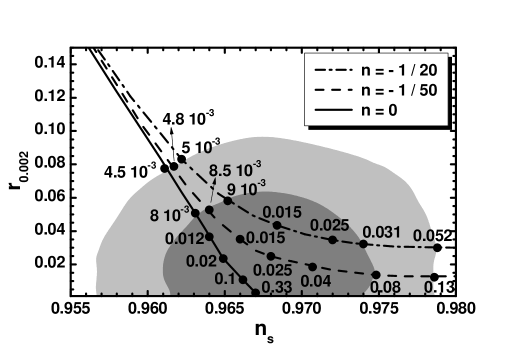
Figure 1: Predicted curves in the $n_{\rm s}-r_{0.002}$ plane for $n=0$ (solid line), $n=-1/50$ (dashed line), $n=-1/20$ (dot-dashed line), $k_{S}=k_{S-}=1$, and various values of $r_{\pm}$ indicated on the curves. The marginalized joint $68\%$ [$95\%$] regions from the Planck, Bicep2/Keck Array  and BAO data are depicted as dark [light] shaded areas.

The structure of $\widehat{V}_{\rm HI}$ as a function of $\phi$ for $\phi_{\star}=1$, $r_{\pm}=0.015$, and the values of $n$ employed in Fig. 1 is displayed in Fig. 2. The values of $n,\lambda$, and $r_{\pm}$, shown in this figure, yield $n_{\rm s}=0.964,0.966$, or $0.968$ and $r=0.033,0.038$, or $0.047$ for $n=0,-1/50$, or $-1/20$ respectively. The corresponding values of $c_{-}$ are $(4.66,5.03,{\rm or}~{}5.6)\times 10^{2}$, whereas the values of $\widehat{\phi}_{\star}$ derived from Eq. (27) are $13.87$, $14.17$, or $14.6$. We verify that observable values of $r$ are associated with transplanckian values of $\widehat{\phi}_{\star}$ in accordance with the Lyth bound [36]. This fact, though, does not invalidate our scenario since the corresponding values of the initial inflaton $\phi$, which is directly related to the superfields $\Phi$ and $\bar{\Phi}$ appearing in the definition of our models in Eqs. (2) and (9) or (10), remain subplanckian – cf. Eq. (38b). We also remark that, in all cases, $\widehat{V}_{\rm HI}^{1/4}(\phi_{\star})$ turns out to be close to the SUSY GUT scale $M_{\rm GUT}\simeq 8.2\times 10^{-3}$, which is imperative – see e.g. Ref. [37] – for achieving values of $r$ close to $0.1$. We finally observe that the slope of $\widehat{V}_{\rm HI}$ close to $\phi=\phi_{\star}$ increases with $|n|$. This is expected to elevate $\widehat{\epsilon}$ – see Sec. 4.2 – and, via Eq. (35c), $r$ too.

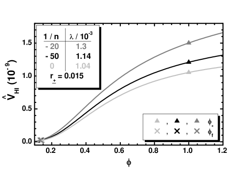
Figure 2: The inflationary potential $\widehat{V}_{\rm HI}$ as a function of $\phi$ for $\phi>0$, $r_{\pm}\simeq 0.015$, and $n=0$, $\lambda=1.04\times 10^{-3}$ (light gray line), $n=-1/50$, $\lambda=1.14\times 10^{-3}$ (black line), or $n=-1/20$, $\lambda=1.3\times 10^{-3}$ (gray line). The values of $\phi_{\star}$ and $\phi_{\rm f}$ are also indicated.

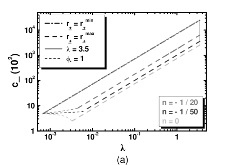
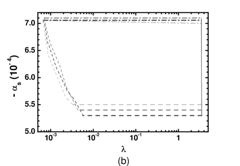
Figure 3: Allowed regions in the $\lambda-c_{-}$ (a) and $\lambda-a_{\rm s}$ (b) plane for $k_{S}=k_{S-}=1$ and $n=0,-1/50$, or $-1/20$ bounded by light, dark, or normal gray lines, respectively. The conventions adopted for the various lines are shown in the panel (a).

To specify further the allowed ranges of the parameters of our models, we plot in Figs. 3-(a) and -(b) the allowed regions in the $\lambda-c_{-}$ and $\lambda-a_{\rm s}$ planes, respectively. The conventions adopted for the various lines are shown in Fig. 3-(a). In particular, the boundary curves of the allowed region for $n=0,-1/50$, or $-1/20$ are represented by light, dark, and normal gray lines, respectively. The dot-dashed and dashed lines correspond, respectively, to the minimal and maximal values of $r_{\pm}$ given in Eq. (LABEL:res1), whereas, on the thin short-dashed lines, the constraint of Eq. (38b) is saturated. The perturbative bound $\lambda\leq 3.5$ (so that the expansion parameter $\lambda^{2}/4\pi\leq 1$) limits the various regions at the opposite end by a thin solid line. For $K={K_{2}}$, the light gray dashed line is expected to be transported to lower values of $c_{-}$, but keeping the same slope. Note that the dot-dashed lines coincide with each other in Fig. 3-(a) and this is almost the case with the dark and light gray dot-dashed lines in Fig. 3-(b) too. We observe that $\lambda/c_{-}$ remains constant for fixed $r_{\pm}$, as expected by the argument below Eq. (50). The required $c_{-}$ for subplanckian excursions of $\phi$ – overall, we obtain $0.014\leq\phi\leq 1$ – is quite large and increases with $|n|$. On the other hand, $|a_{\rm s}|$ remains sufficiently low. Therefore, our models are consistent with the fitting of the data with the $\Lambda$CDM+$r$ model [2].

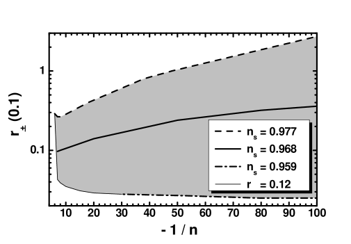
Figure 4: Allowed (shaded) region compatible with Eqs. (32), (34), (37), and (38) in the $(-1/n)-r_{\pm}$ plane for $k_{S}=k_{S-}=1$. The conventions adopted for the various lines are also shown.

Concentrating on the most promising cases with $n<0$, we delineate, in Fig. 4, the overall allowed region of our models by varying continuously $n$ and $r_{\pm}$. The conventions adopted for the various lines are also shown in the figure. In particular, the dashed [dot-dashed] line corresponds to $n_{\rm s}=0.977$ [$n_{\rm s}=0.959$], whereas the solid line is obtained by fixing $n_{\rm s}=0.968$ – see Eq. (37a). On the thin solid boundary line, the bound in Eq. (37b) is saturated. We remark that, as $r_{\pm}$ increases with fixed $n$, $n_{\rm s}$ increases too, while $r$ decreases. This agrees with our findings in Fig. 1. Note that, for $n\geq-1/30$, the thick dot-dashed and the thin solid lines coincide. Overall, for $n_{\rm s}=0.968$ and $\widehat{N}_{\star}\simeq 58$, we find:

$$1.86\lesssim 10^{6}{\lambda\over c_{-}}\lesssim 3.6\>\>\>\mbox{with}\>\>\>8\lesssim-\frac{1}{n}\lesssim 100,\>\>\>1\lesssim{r_{\pm}\over 0.01}\lesssim 3.6\,,\>\>\>\mbox{and}\>\>\>1.8\lesssim{r\over 0.01}\lesssim 12\,.$$ (52)

From these results, we infer that $r_{\pm}$ takes more natural – in the sense of the discussion below Eq. (10) – values (lower than unity) for larger values of $|n|$.

5 The Effective Cut-off Scale

An outstanding trademark of our setting is that perturbative unitarity is retained up to $m_{\rm P}$, despite the fact that the implementation of HI with subplanckian values of $\phi$ requires relatively large values of $c_{-}$ – see Eqs. (43b) and (47b). To show this, we extract the UV cut-off scale $\Lambda_{\rm UV}$ of the effective theory following the systematic approach of Ref. [27]. Let us first clarify that, although the expansions presented below about $\langle{\phi}\rangle=M\ll 1$ are not valid [26] during HI, we consider the resulting $\Lambda_{\rm UV}$ as the overall cut-off scale of the theory, since reheating is regarded as an unavoidable stage of the inflationary dynamics [27].

The canonically normalized inflaton can be written as follows – see Eq. (26b):

$$\widehat{\delta\phi}=\langle{J}\rangle\delta\phi\>\>\>\mbox{with}\>\>\>\delta\phi\equiv\phi-M\>\>\>\mbox{and}\>\>\>\langle{J}\rangle=\sqrt{\langle{\kappa_{+}}\rangle}\simeq\sqrt{c_{-}/\langle{f_{\cal R}}\rangle}\,,$$ (53)

where the last (approximate) equality is valid only for $r_{\pm}\ll 1/N$ – see Eq. (25). Note, in passing, that the mass of $\widehat{\delta\phi}$ at the vacuum is calculated to be

$$\widehat{m}_{\rm\delta\phi}=\left\langle\widehat{V}_{\rm HI0,\widehat{\phi}\widehat{\phi}}\right\rangle^{1/2}=\left\langle\widehat{V}_{\rm HI0,\phi\phi}/J^{2}\right\rangle^{1/2}\simeq\frac{\lambda M}{\sqrt{2c_{-}(1-Nr_{\pm})}}$$ (54)

with numerical values $(1.5-3.3)\times 10^{-8}$ along the solid line of Fig. 4 where $n_{\rm s}\simeq 0.968$. Given that $\langle{f_{\cal R}}\rangle\simeq 1$, $|n|\ll 1$, and $\lambda/c_{-}$ is fixed – see Eqs. (44) and (48) –, the variation of $\widehat{m}_{\rm\delta\phi}$ is mainly generated by the variation of $r_{\pm}$. In other words, for fixed $n$, $\widehat{m}_{\rm\delta\phi}$ depends only on $r_{\pm}$ and not on $\lambda,M,c_{-}$, or $c_{+}$ separately. Note that the resulting values of $\widehat{m}_{\rm\delta\phi}$ are almost two orders of magnitude lower than the values obtained in similar models [8, 18, 9] and so the successful activation of the mechanism of non-thermal leptogenesis [28] is an important open issue.

The fact that $\widehat{\delta\phi}$ does not coincide with $\delta\phi$ in Eq. (53) – contrary to the case of standard non-minimal HI [25, 26] – ensures that our models are valid up to $m_{\rm P}=1$ – cf. Ref. [10]. Taking into account Eq. (26a) and calculating the action ${\sf S}$ in Eq. (12a) on the path of Eq. (5) with spatially constant values of $\phi$, we find

$${\sf S}=\int d^{4}x\sqrt{-\widehat{\mathfrak{g}}}\left(-\frac{1}{2}\widehat{\mathcal{R}}+\frac{1}{2}\,J^{2}\dot{\phi}^{2}-\widehat{V}_{\rm HI0}+\cdots\right),$$ (55a)

where $$J \widehat{V}_{\rm HI0} J^{2} \phi=\langle{\phi}\rangle=M\simeq 0 \widehat{\phi} \simeq\widehat{\delta\phi}$$ is given in Eq. (26b) and in Eq. (19). Expanding about and expressing the result in terms of () using Eq. (53), we obtain

$$J^{2}\dot{\phi}^{2}=\left(1-r_{\pm}\widehat{\phi}^{2}+3Nr_{\pm}^{2}\widehat{\phi}^{2}+r_{\pm}^{2}\widehat{\phi}^{4}-5Nr_{\pm}^{3}\widehat{\phi}^{4}+\cdots\right)\dot{}\widehat{\phi}^{2}.$$ (55b)

If we insert Eq. (11) into Eqs. (24) and (26b) and repeat the same expansion, we get the notorious term $$2Nc_{\cal R}^{2}\widehat{\phi}^{2} \Lambda_{\rm UV}\ll 1 c_{\cal R} c_{\cal R} r_{\pm} c_{+} c_{-} \widehat{V}_{\rm HI0} \widehat{\phi}$$ [25, 26], which entails for large . In our case, however, is replaced by which remains low enough – although and may be large – rendering the effective theory unitarity safe. Expanding similarly in terms of , we have

$$\widehat{V}_{\rm HI0}=\frac{\lambda^{2}\widehat{\phi}^{4}}{16c_{-}^{2}}\left(1-2(1+n)r_{\pm}\widehat{\phi}^{2}+(3+5n+2n^{2})r_{\pm}^{2}\widehat{\phi}^{4}-\cdots\right)\cdot$$ (55c)

This expression, for $n=0$, reduces to the one presented in Ref. [10], whereas the expression for $J$ in Eq. (55b) differs slightly from the corresponding one in this reference, due to the different normalization of $\phi$ in Eqs. (24) and (26b). Since the positivity of $\kappa_{-}$ in Eq. (24) entails $r_{\pm}<1/N<1$, our overall conclusion is that our models do not face any problem with perturbative unitarity up to $m_{\rm P}$.

6 Conclusions

We presented models of Higgs inflation in SUGRA, which accommodate inflationary observables covering the ‘sweet’ spot of the recent joint analysis of the Bicep2/Keck Array and Planck data. Our models, at the renormalizable level, are tied to a unique superpotential determined by an $R$ and a gauge $U(1)_{B-L}$ symmetry. We selected two possible Kähler potentials $K$, one logarithmic and one semi-logarithmic – see Eqs. (9) and (10) –, which respect the symmetries above and a mildly violated shift symmetry. Both $K$’s lead to practically identical inflationary models. The key-point in our proposal is that the coefficient $c_{-}$ of the shift-symmetric term in the Kähler potentials does not appear in the supergravity inflationary scalar potential expressed in terms of the original inflaton field, but strongly dominates the canonical normalization of this inflaton field. The inflationary scenario depends essentially on three free parameters ($n$, $\lambda/c_{-}$, and $r_{\pm}$), which are constrained to natural values leading to values of $n_{\rm s}$ and $r$ within their $1-\sigma$ observational margins. Indeed, adjusting these parameters in the ranges $n=-(0.1-0.01)$, $\lambda/c_{-}=(1.86-3.6)\times 10^{-6}$, and $r_{\pm}=0.01-0.036$, we obtain $n_{\rm s}\simeq 0.968$ and $0.018\lesssim r\lesssim 0.12$ with negligibly small values of $|a_{\rm s}|$. Imposing a lower bound on $c_{-}$, we succeeded to realize HI with subplanckian values of the original inflaton, thereby stabilizing our predictions against possible higher order corrections in the superpotential and/or the Kähler potentials. Moreover, the corresponding effective theory remains trustable up to $m_{\rm P}$. We also showed that the one-loop RCs remain subdominant for a convenient choice of the renormalization scale. Finally, the scale of $U(1)_{B-L}$ breaking can be identified with the SUSY GUT scale and the mass $\widehat{m}_{\rm\delta\phi}$ of the normalized inflaton is confined in the range $(1.5-3.3)\times 10^{-8}$.

As a last remark, we would like to point out that, although we have restricted our discussion to the $G_{B-L}$ gauge group, the HI analyzed in this paper has a much wider applicability. It can be realized within other SUSY GUTs too based on a variety of gauge groups – such as the left-right, the Pati-Salam, or the flipped $SU(5)$ group – provided that a conjugate pair of Higgs superfields is used in order to break the symmetry. In these cases, the inflationary predictions are expected to be quite similar to the ones discussed here. The discussion of the stability of the inflationary trajectory may, though, be different, since different Higgs superfield representations may be involved in implementing the GUT gauge symmetry breaking to $G_{\rm SM}$.