The spatio-temporal spectrum of turbulent flows

Abstract

Identification and extraction of vortical structures and of waves in a disorganised flow is a mayor challenge in the study of turbulence. We present a study of the spatio-temporal behavior of turbulent flows in the presence of different restitutive forces. We show how to compute and analyse the spatio-temporal spectrum from data stemming from numerical simulations and from laboratory experiments. Four cases are considered: homogeneous and isotropic turbulence, rotating turbulence, stratified turbulence, and water wave turbulence. For homogeneous and isotropic turbulence, the spectrum allows identification of sweeping by the large scale flow. For rotating and for stratified turbulence, the spectrum allows identification of the waves, precise quantification of the energy in the waves and in the turbulent eddies, and identification of physical mechanisms such as Doppler shift and wave absorption in critical layers. Finally, in water wave turbulence the spectrum shows a transition from gravity-capillary waves to bound waves as the amplitude of the forcing is increased.

1 Introduction

Turbulence can be characterised as the disorganised spatio-temporal and chaotic evolution of a flow, by the development of multi-scale structures, and in many cases by intermittency (i.e., the development of localised energetic structures in space and time, see e.g., Biferale04 ). Although turbulence is a spatio-temporal phenomena, limitations in experiments and in numerical simulations led studies either towards spatial characterisation of the flows (e.g., using two-point spatial structure functions, or the wavenumber energy spectrum), or towards temporal characterisation (e.g., using the frequency spectrum of time series). On the one hand, computers excel in the former approach, as velocity fields can be obtained today in numerical simulations with relatively high spatial resolution, but temporal cadence tends to be low as a result of the high computational cost of writing large files in supercomputers. On the other hand, experiments excel in the latter. Long time series are relatively easier to obtain, while spatial resolution in the laboratory is often limited.

This led to different approaches to tackle the study of turbulence. While some authors focused on spatial properties and scaling laws, others considered the evolution of individual structures such as vortex filaments or hairpin vortices Hussain86 ; Rogers87 . Identification of individual (and coherent) structures in the disorganised flow has always been a major quest for turbulence research. Techniques such as the proper orthogonal decomposition Berkooz93 allowed spatio-temporal tracking of these structures, and the generation of low dimensional models for some turbulent flows Smith05 .

In the presence of restitutive forces (such as gravity and buoyancy in a stratified fluid, or the Coriolis force in a rotating fluid), the flow can also sustain waves that make the problem stiff: for strong enough restitutive forces, waves introduce a fast time scale and their amplitudes are slowly modulated by the evolution of the vortical structures. The ability of waves to affect the properties of turbulent flows has been recognised for a long time; as a few examples, it is now clear they can alter the diffusion process in the ocean Woods80 , make the flow anisotropic Cambon89 ; Waleffe93 ; Cambon97 , and change the very nature of nonlinear interactions Nazarenko . Understanding the effect of waves in turbulence has implications in geophysical, astrophysical, and industrial flows. Although separating waves from eddies in a turbulent flow has been deemed impossible in the past Stewart69 , multiple advances allowed a formal treatment of turbulence in the presence of waves Cambon89 ; Waleffe93 ; Nazarenko , as well as some ways to decompose a turbulent flow into wave and vortical motions (see, e.g., Smith02 ; Bourouiba08 ; Sen12 ). These decompositions are based on spatial information and on the dispersion relation of the waves, defining Fourier modes with zero wave frequency as vortical or “slow”, and modes with non-zero wave frequency as waves or “fast”, with this approximation being valid only for very strong restitutive forces.

The development of experimental techniques such as Particle Image Velocimetry (PIV, see Adrian91 ) or fringe projection profilometry (including Fourier Transform Profilometry or FTP Maurel09 ; Cobelli09 , and Empirical Mode Decomposition Profilometry or EMDP Lagubeau15 ), and the growth of computing power (as well as the development of new technologies such as burst buffers for the next generation of supercomputers Liu12 ), allowed obtaining experimental and numerical data with space and time information. In this paper we will focus on recent methods developed to detect and extract waves from the turbulent velocity field (and in the case of water waves, also from the turbulent surface deformation field), resulting from the superposition and nonlinear interaction of waves and eddies.

Different methods can be employed to identify the presence of waves in a turbulent flow, provided data in the spatial and temporal domain are available. This is needed as waves are defined by their spatio-temporal structure, i.e., by their dispersion relation. One approach, recently used in experiments of rotating turbulence Campagne15 , is to calculate the two-point spatial correlation of the temporal Fourier transform of the velocity field, obtained from PIV measurements. In Campagne15 , the authors were able to quantify anisotropy and to identify inertial waves. Another approach is to use the fact that bounded domains give rise to resonant frequencies and look for peaks in the temporal Fourier spectrum, as was done in experiments of rotating turbulence Bewley07 ; Rieutord12 in both cylindrical and square containers (see also Lamriben11 for a recent study in a closed container considering temporal information as well as the full spatial fields). Yet another approach is to study the decorrelation time of different spatial modes, and to see which are decorrelated by wave dynamics (i.e., in one period of the waves) and which are decorrelated by sweeping (i.e., in one turnover time of the large-scale flow). This was done for magnetohydrodynamic (MHD) turbulence simulations Servidio11 and for rotating turbulence simulations Favier10 ; Clark14a . Using a similar technique, some authors looked for peaks in the frequency spectrum of particular modes, as these should be located at the frequencies corresponding to the wave dispersion relation; these studies were conducted in MHD turbulence Dmitruk09 and in stratified rotating turbulence Lindborg07 . Finally, some observational studies of stratified turbulence in the oceans attempted identification of waves by studying Lagrangian trajectories in the fluid Dasaro00 .

Recently, computational and experimental advances made it possible to calculate the complete spatio-temporal spectrum for all modes resolved in an experiment or a simulation. This spectrum has been calculated, e.g., in experiments Cobelli11 ; Aubourg15 and simulations Clark14b of water waves, in experiments of vibrating plates Cobelli09 ; Yokoyama14 , in experiments Yarom14 and simulations Clark14a of rotating turbulence, in simulations of magnetohydrodynamic turbulence Meyrand15 , in simulations of stratified turbulence Clark15 , and in simulations of quantum turbulence Nazarenko06a ; Nazarenko06b ; Clark15b for flows of superfluid helium or for Bose-Einstein condensates. These studies allowed identification of wave modes, a precise quantification of how much energy is present in these modes as a function of the length scale, and identification of physical effects associated with the presence of waves.

Similar techniques were developed in other areas, specially in plasma physics and in space physics. Experimental investigations of space plasma turbulence have recently turned from single-point measurements (which suffered invariably from ambiguities in disentangling temporal and spatial variations) to multipoint measurements Sahraoui10 ; Sahraoui11 . A paradigmatic example of this is the CLUSTER mission, which comprises an in situ investigation of the Earth’s magnetosphere using four identical spacecraft simultaneously to distinguish between spatial and temporal variations Escoubet . The multi-spacecraft mission allows combination of multiple time series recorded simultaneously at different points in space to estimate the corresponding energy density in wavenumber-frequency space Sahraoui11 . More recently, data from the Coronal Multi-channel Polarimeter (CoMP) allowed reconstruction of the spatio-temporal spectrum and identification of Alfvén waves in the solar corona Morton15 .

In the following sections we show how to compute and analyse the spatio-temporal spectrum of turbulent flows, from numerical simulations and experiments. We focus on four cases. Two were reported extensively in Clark14a ; Clark15 and are briefly summarised here, and correspond respectively to numerical studies of rotating turbulence, and of stratified turbulence. The spatio-temporal spectrum allows identification of the waves, quantification of the energy in the waves and in the turbulent eddies, and identification of physical mechanisms such as Doppler shift and critical layer absorption. The two other examples are new. We present the spatio-temporal spectrum of numerical simulations of homogeneous and isotropic turbulence, and the spatio-temporal spectrum of laboratory experiments of water wave turbulence. In the former case, the analysis allows identification of sweeping of the small scale vortices by the large scale flow. In the latter, we show a transition from gravity-capillary wave turbulence to bound waves as the amplitude of the forcing is increased.

2 Methods

2.1 Numerical simulations

To compute spatio-temporal resolved spectra in three-dimensions (3D), we will consider data stemming from direct numerical simulations of isotropic, rotating, and stratified turbulence. In the most general case, the evolution of a rotating and stratified fluid in the Boussinesq approximation is described by

$$\frac{\partial\mathbf{u}}{\partial t}+\mathbf{u}\cdot\mathbf{\nabla}\mathbf{u}-\nu\nabla^{2}\mathbf{u} =-f\hat{z}\times\mathbf{u}-N\theta\hat{z}-{\bf\nabla}p+\mathbf{F},$$ (1)

$$\frac{\partial\theta}{\partial t}+\mathbf{u}\cdot\mathbf{\nabla}\theta-\kappa\nabla^{2}\theta =N\mathbf{u}\cdot\hat{z},$$ (2)

along with the incompressibility condition

$$\nabla\cdot\mathbf{u}=0,$$ (3)

where $\mathbf{u}$ is the velocity field, $\theta$ is the potential temperature fluctuations, $p$ is the pressure (including the centrifugal contribution), $f=2\Omega$ (where $\Omega$ is the rotation frequency, and the axis of rotation is in the $\hat{z}$ direction), $N$ is the Brunt-Väisälä frequency (note that stratification is also in the $\hat{z}$ direction), $\mathbf{F}$ is an external mechanical forcing, $\nu$ is the kinematic viscosity, and $\kappa$ the thermal diffusivity (for simplicity we take $\kappa=\nu$, i.e., a Prandtl number $Pr=\nu/\kappa=1$). By linearising the equations, it is straightforward to verify that inertia-gravity waves are solutions to these equations, with dispersion relation

$$\omega(\mathbf{k})=\pm\frac{\sqrt{N^{2}k^{2}_{\perp}+f^{2}k^{2}_{\parallel}}}{k},$$ (4)

where $k_{\perp}=(k^{2}_{x}+k^{2}_{y})^{1/2}$, $k_{\parallel}=k_{z}$, and $k=(k^{2}_{\perp}+k^{2}_{\parallel})^{1/2}$.

Simulation	Re	Fr	Ro
Isotropic turbulence	5000	–	–
Rotating turbulence	5000	–	0.015
Stratified turbulence	9700	0.01	–

Table 1: Dimensionless parameters for the three different numerical simulations. Re is the Reynolds number, Fr is the Froude number, and Ro is the Rossby number.

All cases considered can be recovered from these equations. The incompressible Navier-Stokes equation used for isotropic and homogeneous turbulence is obtained from Eq. (1) for $N=f=0$. In this case there are no waves, and only vortical structures are present in the flow. Equation (2) then reduces to the equation for a passive scalar.

The purely rotating case is obtained from Eq. (1) for $N=0$. As the only restitutive force is the Coriolis force, the system can sustain inertial waves, which from Eq. (4) follow the dispersion relation given by

$$\omega_{R}(\mathbf{k})=\pm\frac{fk_{\parallel}}{k}.$$ (5)

Finally, the purely stratified flow is obtained for $f=0$. Equation (4) now becomes the dispersion relation of internal gravity waves,

$$\omega_{S}(\mathbf{k})=\pm\frac{Nk_{\perp}}{k}.$$ (6)

To solve these equations we use GHOST Gomez05a ; Gomez05b ; Mininni11 , a parallel 3D pseudospectral code with periodic boundary conditions, which uses either a second or fourth order Runge-Kutta method for the time evolution. A spatial resolution of $512^{3}$ points in a regular grid is used in all cases. In all simulations the fluid starts from rest, and a constant in time forcing is applied (constant forcing is used to prevent introduction of external timescales to the system, that may be visible in the time spectrum). The systems are then allowed to reach a turbulent steady state. Once this stage is reached, we let the systems run for at least 10 large-scale turnover times, in order to get enough statistics on the slower timescales of the system. For isotropic and homogeneous turbulence, and for stratified turbulence, we use an isotropic and randomly generated three dimensional forcing acting at $k=1$. For rotating turbulence we use Taylor-Green forcing with $\mathbf{F}=f_{0}(\sin x\cos y\cos z\hat{x}-\cos x\sin y\cos z\hat{y})$. See Clark14a ; Clark15 for more details of the simulations of rotating and of stratified turbulence.

The dimensionless parameters that describe these systems are the Reynolds number $\mathrm{Re}=U_{rms}L/\nu$, where $U_{rms}$ is the r.m.s. velocity and $L$ the energy-containing length scale, the Rossby number $\mathrm{Ro}=U_{rms}/(fL)$ which measures the relative strength of rotation, and the Froude number $\mathrm{Fr}=U_{rms}/(NL)$ which measures the relative strength of stratification. The values of these dimensionless parameters for the three simulations considered below are shown in Table 1.

2.2 Experimental setup

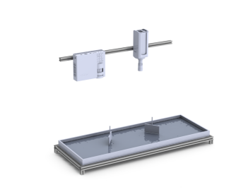
Figure 1: Experimental setup to generate water wave turbulence. The tank of $(200\times 80)$ cm² is filled with water tainted with titanium dioxide to make it opaque and allow projection of a pattern on its surface. The two wavemakers driven by independent servomotors (not shown) excite random perturbations of the free surface. A high resolution projector projects a fringe pattern of known characteristics (not shown in the scheme), and a fast speed camera captures the pattern deformation. The profilometry technique then allows for reconstruction of the surface deformation with high temporal cadence and high spatial resolution Maurel09 ; Cobelli09 ; Lagubeau15 .

The data to compute the spatio-temporal resolved spectrum of water wave turbulence stems from an experimental setup to study waves in the free surface of a liquid (see Fig. 1). The setup consists of a $(200\times 80)$ cm² tank filled with water with depth at rest $h_{0}=5$ cm. Waves are generated in the tank by two piston-type wave makers ($20$ cm large and $\approx 1$ cm immersed) independently driven by two linear tubular servomotors. Two independent random signals with frequency range between 0 and $2.7$ Hz and with amplitude $A$ are used to control the wavemakers. Three experiments were performed, one with $A=1$ cm, another one with $A=2$ cm, and a third one with $A=3$ cm. Under this set of conditions, and in the absence of wave breaking, waves should follow the linear dispersion relation of gravity-capillary waves

$$\omega_{W}(k)=\sqrt{\tanh(h_{0}k)\left(gk+\frac{\gamma}{\rho}k^{3}\right)},$$ (7)

where $\gamma$ is the surface tension, and $\rho$ the density of water.

The surface height deformation $h(x,y,t)$ is obtained with high temporal cadence and high spatial resolution using a fringe projection profilometry technique Maurel09 ; Cobelli09 . Titanium dioxide is added to the water as dye, in order to render the free surface light diffusive without changing significatively its rheological properties Przadka2012 and be able to project onto it a controlled pattern by means of a high-resolution, high-contrast projector. A fast speed camera, with a resolution of $1024\times 1024$ px² and inspecting an area of $(41.6\times 41.6)$ cm², is then used to capture deformations of the pattern as the result of the surface deformation. The size of the projected pixel, about $0.04$ cm, sets the spatial resolution. The temporal resolution is $1/F$, where $F$ is the acquisition frequency (in our case $F=250$ Hz). The profilometry technique reconstructs the height of the surface $h(x,y,t)$ from the distortion in the patterns captured by the camera.

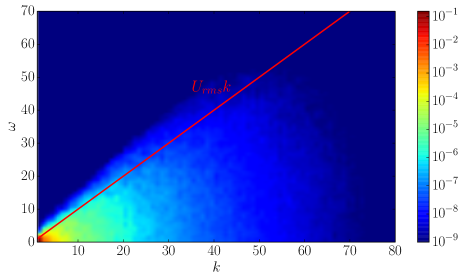
Figure 2: Spatio-temporal spectrum $E(k,\omega)$ in a numerical simulation of isotropic and homogeneous turbulence. The solid curve corresponds to $\omega=U_{rms}k$. As a result of sweeping of the small scale eddies by the large scale flow, most of the energy is concentrated in the region $\omega\leq U_{rms}k$.

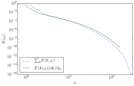
Figure 3: Frequency spectrum $E(\omega)$ for the homogeneous and isotropic turbulence simulation, calculated directly as $E(\omega)=\sum_{k}E(k,\omega)$ (dashed blue line). The solid (green) line is obtained by transforming the spatial spectrum $E(k)$ into a frequency spectrum $E(k(\omega))d\omega/dk$ using the sweeping relation $\omega=U_{rms}k$. As sweeping is the dominant Eulerian time scale in the system, one spectrum can be recovered from the other with reasonable agreement of both spectra in the inertial range.

2.3 Construction of the spatio-temporal spectrum

In principle, computation of the spatio-temporal spectrum reduces to computing Fourier transforms of the space and time resolved numerical or experimental data. In practice, some provisions may be made to allow for efficient storage and correct handling of the data.

First of all, both in numerical simulations and in experiments, the acquisition frequency must be at least two times larger than the frequency of the fastest waves one wants to study, and the total time of acquisition should be larger than the period of the slowest waves in the system, and larger than the turnover time of the slowest eddies.

In numerical simulations storage constraints (both in space as well as in I/O speed) make it difficult to store the velocity fields at all points in space with high temporal cadence (e.g., every time step, or every a very few time steps), specially at high spatial resolutions. As a result, we store the Fourier transform of the velocity field $\hat{\bf u}({\bf k},t)$ with high temporal cadence, and for selected Fourier modes ${\bf k}$. In most cases it suffices to store all Fourier modes in three planes (corresponding to the planes with $k_{x}=0$, $k_{y}=0$, and $k_{z}=0$). This allows reconstruction of the spatio-temporal energy spectrum in three planes $E(k_{x}=0,k_{y},k_{z},\omega)$, $E(k_{x},k_{y}=0,k_{z},\omega)$, and $E(k_{x},k_{y}=0,k_{z},\omega)$, where, e.g., the first is computed from the spatial Fourier modes of the velocity field in the plane with $k_{x}=0$ as

$$E(k_{x}=0,k_{y},k_{z},\omega)=\frac{1}{2}\left|\int{\hat{\bf u}(k_{x}=0,k_{y},k_{z},t)e^{-i\omega t}dt}\right|^{2}.$$ (8)

Note that in all cases the computation results in a four dimensional spectrum, or in multiple three dimensional spectra that are better studied by plotting slices for constant values of the wavenumber Cartesian components or of the frequency. Furthermore, if the spectrum is isotropic (in the absence of external forces) or axisymmetric (in the rotating or stratified cases), symmetry considerations allow for reconstruction of the isotropic spectrum $E(k,\omega)$ or of the axisymmetric spectrum $E(k_{\perp},k_{\parallel},\omega)$ from these three spectra. (see, e.g., Davidson ).

When the data is not periodic (as is the case with the spatial data in experiments, or with temporal data in both experiments and in simulations) it is advisable to use a window function to avoid introducing artifacts when the Fourier transforms are performed, and to mitigate spectral leakage. In the following, a flat top filter will be used when computing the temporal Fourier transforms for all the data coming from simulations. For the experimental data, a Hanning window will be used in both space and time. Furthermore, in experiments it is relatively easier to obtain long time signals; this allows us to perform a Welch average in order to reduce noise in the frequency spectra.

3 Results

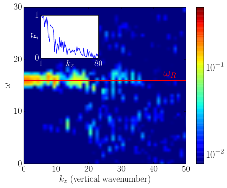
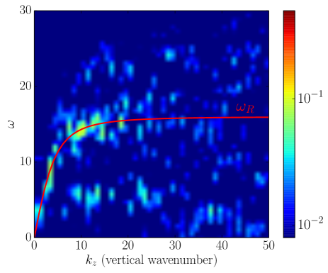
Figure 4: Spatio-temporal energy spectrum $E(k_{x}=0,k_{y},k_{z},\omega)$ from numerical simulations of rotating turbulence. Two slices are shown for fixed values of $k_{y}$. Top: $k_{y}=0$, and bottom: $k_{y}=1$. The dispersion relation of inertial waves, $\omega_{R}({\bf k})$, is shown by the solid line. For small wavenumbers most of the energy is concentrated around this dispersion relation. Inset: Ratio of the energy in the vicinity of the modes satisfying the dispersion relation, to the total energy in the same wavenumber.

3.1 Homogeneous and isotropic turbulence

In the absence of restitutive forces, an incompressible fluid cannot sustain waves. Isotropic and homogeneous turbulence can then be characterised by two timescales which follow from the Navier-Stokes equation: the eddy turnover time at the scale $\ell$, given by $\tau_{\ell}=\ell/u_{\ell}$ where $u_{\ell}$ is the characteristic velocity of an eddy of size $\ell$, and the sweeping time, given by $T=\ell/U_{rms}$, which describes the sweeping of vortices of size $\ell$ by the flow at the largest scale. The former is related to the local interaction of modes in Fourier space, i.e., of eddies of similar sizes, while the latter deals with the non-local interaction in Fourier space resulting from the advection of small eddies by the energy containing ones. It has been theorised Tennekes75 ; Chen89 and later shown Nelkin90 ; Sanada92 that the temporal decorrelation of Fourier modes of the Eulerian velocity field in homogeneous and isotropic turbulence is determined by this sweeping. In numerical simulations sweeping is often quantified by computing the decorrelation time of individual Fourier modes, using two-time correlation functions. The spatio-temporal spectrum of isotropic and homogeneous turbulence has not been considered so far to quantify its effect.

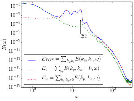
Figure 5: Frequency spectra of kinetic energy in the simulation of rotating turbulence. Here $E_{v}(\omega)$ (dashed green line) has only the contribution from the vortical modes, while $E_{w}(\omega)$ (dash-dotted red line) has the contribution of the so-called “wave” modes (i.e., modes with $k_{z}>0$). The total frequency spectrum $E_{TOT}$ (solid blue line) is obtained by summing the spatio-temporal spectrum over all wavenumbers. The largest peak in $E_{w}$ corresponds to a frequency $2\Omega$, indicated by the arrow. The contribution of the eddies dominate the smaller frequencies with $\omega\lesssim 4$, where waves are too slow and the two-dimensional vortices are strong. For frequencies larger than $2\Omega$ modes cannot be described as inertial waves and eddies must dominate all spectra.

Figure 2 shows the spatio-temporal energy spectrum computed using the velocity field stemming from the simulation of isotropic and homogeneous turbulence (see Table 1). The thick red line indicates the relation $\omega=U_{rms}k$, corresponding to the frequency of sweeping by a flow with constant velocity $U_{rms}$. Sweeping appears in the spectrum as the concentration of energy along and below this line. Structures of size $\ell\sim 1/k$ are advected by the large-scale velocity which roughly fluctuates between 0 and $\approx U_{rms}$. In other words, at a given wavenumber $k$, all frequencies are excited up to $\omega=U_{rms}k$, and not just the frequency corresponding to the eddy turnover time at that wavenumber, $\omega_{k}\sim 1/\tau_{\ell}$. Note that as was pointed out in Tennekes75 ; Chen89 , the dominance of the sweeping time as the Eulerian decorrelation time, over the eddy turnover time, is needed for the frequency spectrum of isotropic and homogeneous turbulence to be $E(\omega)\sim\omega^{-5/3}$, provided the wavenumber spectrum is Komogorov’s $E(k)\sim k^{-5/3}$.

Indeed, the spatio-temporal spectrum in Fig. 2 allows direct computation of both spectra, $E(\omega)$ and $E(k)$, without relying on extra assumptions such as the Taylor hypothesis. We can actually put this fact to good use to further verify that the dominant timescale in the system is the one given by the sweeping mechanism. In Fig. 3 we show $E(\omega)$ computed as $E(\omega)=\sum_{k}E(k,\omega)$ (i.e., computing it directly from the spatio-temporal spectrum), compared with the spectrum $E(\omega(k))d\omega/dk$ obtained from the spatial spectrum $E(k)$ using Taylor (or sweeping) hypothesis (i.e., from a change of variables using the relation $\omega=U_{rms}k$). The good agreement between the inertial ranges of the two spectra confirms that sweeping is the dominant time scale for the Eulerian velocity. Note also the presence of the well known bottleneck in the dissipative range of the spatial spectrum.

3.2 Rotating turbulence

Rotation breaks down the isotropy of the flow, as the axis of rotation establishes a preferred direction. The Coriolis term also acts as a restitutive force that allows the fluid to sustain inertial waves. For strong enough rotation, these waves are much faster than the eddies, at least for a subset of all Fourier modes corresponding to modes with $k_{\parallel}\neq 0$ (as for $k_{\parallel}=0$ the dispersion relation of the waves vanishes), and to modes with $k<k_{\Omega}$ (where $k_{\Omega}$ is the Zeman wavenumber for which the eddies become as fast as the waves and the flow recovers isotropy Mininni12 ). Non-linear resonant interactions between triads of these waves then become the preferred energy transfer mechanism Newell69 ; Cambon89 ; Waleffe93 . Given three modes with wave vectors ${\bf k}$, ${\bf p}$, and ${\bf q}$, they can interact and transfer energy if

$${\bf k}+{\bf p}+{\bf q}=0,$$ (9)

$$\omega_{R}({\bf k})+\omega_{R}({\bf p})+\omega_{R}({\bf q})=0.$$ (10)

The last relation is the resonant condition. These relations dictate that energy in a rotating flow is transferred preferentially towards modes with smaller $k_{\parallel}$ Waleffe93 (as modes with $k_{\parallel}=0$ trivially satisfy the resonant condition), resulting in a growth of the anisotropy and the quasi-bidimensionalization of the flow.

Multiple wave turbulence theories have been proposed for rotating turbulence based on these conditions (see, e.g., Cambon89 ; Cambon97 ; Cambon04 ). However, the theories often assume the rapidly rotating limit in which waves overshadow the eddies completely. Thus, the slow or vortical modes with $k_{\parallel}=0$ and the modes with $k\approx k_{\Omega}$ cannot be properly described within the framework of these theories. Moreover, in simulations and experiments the discrimination between waves and eddies often reduces to considering modes with $k_{\parallel}\approx 0$ (for which $\omega_{R}({\bf k})\approx 0$) as eddies, and all other modes as waves. Computation of the spatio-temporal spectrum, which has been recently performed for numerical simulations Clark14a and for experimental data Yarom14 , allows for a proper identification of the waves and a quantification of their relevance at different scales.

The spatio-temporal spectrum of the kinetic energy $E(k_{x},k_{y},k_{z},\omega)$ for the simulation of rotating turbulence (see Table 1) is shown in Fig. 4, for $k_{x}=0$ and for two fixed values of $k_{y}$ ($k_{y}=0$ and $k_{y}=1$). As mentioned in Sec. 2.3, compared with results previously shown in Clark14a , the spectrum in Fig. 4 was computed using a flat top window to reduce spectral leakage. Note that unlike the spectrum in Fig. 2, sweeping effects cannot be observed in these spectra. Instead, energy is accumulated near modes satisfying the dispersion relation of inertial waves. In Fig. 4 we also show the ratio of the energy in these modes to the total energy in the same wavenumber

$$F(k_{z})=\frac{E(k_{x}=0,k_{y}=0,k_{z},\omega=\omega_{R})}{\int E(k_{x}=0,k_{y}=0,k_{z},\omega)d\omega}$$ (11)

(in practice, the energy of the modes satisfying the dispersion relation is computed with a finite width between $\omega_{R}\pm 3$). For wavenumbers up to $k_{z}\approx 30$, modes compatible with waves concentrate a large fraction of the energy. However, for $k_{z}>30$ the fraction of the energy in the waves drops quickly to less than $\approx 10\%$. Interestingly, the wavenumber $k_{\Omega}$ for which waves become negligible and isotropy is recovered is much larger in this simulation, $k_{\Omega}\approx 460$ (see Clark14a ). In fact, it can be shown that waves become subdominant in the spatio-temporal spectrum as soon as the sweeping time becomes of the same order as the wave period Clark14a . Thus, at moderate Rossby numbers, eddies (although strongly anisotropic) are relevant for the energetics of inertial-range rotating turbulence and cannot be neglected.

To further quantify the contribution of vortical modes and of eddies to the energy spectrum, we can estimate a frequency spectrum of kinetic energy from the slices of the $E({\bf k},\omega)$ spectrum. As an example, from the three-dimensional spectrum $E(k_{x}=0,k_{y},k_{z},\omega)$, we can estimate a “total” frequency spectrum as

$$E_{TOT}(\omega)=\sum_{k_{y},k_{z}}E(k_{x}=0,k_{y},k_{z},\omega),$$ (12)

a “vortical” spectrum that has only contributions from the slow or vortical modes (i.e., the modes with $k_{z}=0$, such that the wave frequency is $\omega_{R}=0$),

$$E_{v}(\omega)=\sum_{k_{y}}E(k_{x}=0,k_{y},k_{z}=0,\omega),$$ (13)

and finally, the frequency spectrum of all the modes which are often associated with fast or wave modes in wave turbulence theories Smith02 ; Bourouiba08 ; Sen12

$$E_{w}(\omega) =\sum_{k_{y},k_{z}>0}E(k_{x}=0,k_{y},k_{z},\omega)$$

$$=E_{TOT}(\omega)-E_{v}(\omega).$$ (14)

Note that $E_{w}(\omega)$, although often associated with the spectrum of the waves, contains contributions from modes in Fig. 4 which do not satisfy the dispersion relation $\omega_{R}({\bf k})$.

The resulting spectra are shown in Fig. 5. The spectrum of vortical modes $E_{v}$ gives the largest contribution to $E_{TOT}$ for frequencies $\omega\lesssim 4$, where the strong two-dimensional modes carry most of the energy. For $4<\omega\leq 2\Omega$, $E_{w}$ becomes dominant and wave modes give the largest contribution to the energy. However, for $\omega>2\Omega$ there are no inertial waves (as the frequency of inertial waves has an upper bound of $2\Omega$), and all modes that contribute to the spectra must be associated with vortical motions (even for $E_{w}$). All the spectra in this range then show the same behavior. The coexistence of multiple timescales in this system does not allow a simple transformation of the wavenumber spectrum into the frequency spectrum, as was done in Sec. 3.1 for isotropic and homogeneous turbulence.

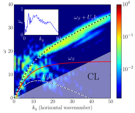
Figure 6: Spatio-temporal spectrum of the potential energy, $E_{\theta}(k_{x}=0,k_{y},k_{z}=10)$ in the simulation of stratified turbulence. The dispersion relation of internal gravity waves, $\omega_{S}({\bf k})$, is indicated by the solid line. Also shown are two Doppler-shifted dispersion relations, corresponding to the horizontal r.m.s. velocities $U_{y}=\pm 0.4$, and indicated by the dashed and dash-dotted lines. Energy is not concentrated around the linear dispersion relation, instead it is spread in the fan between these two Doppler-shifted branches. Moreover, the distribution of energy is not uniform as waves with $\omega<U_{y}k_{y}$ are absorbed by the mean flow in Critical Layers (indicated by the shaded area labeled “CL”). Note the almost complete lack of energy in this region. Inset: fraction of the energy contained within the two Doppler shifted branches.

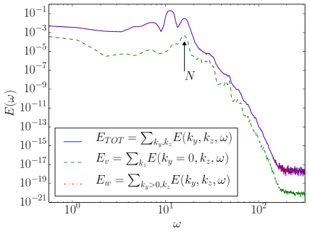
Figure 7: Frequency spectra of potential energy in the simulation of stratified turbulence. In this case $E_{v}$ (dash-dotte red line) has the contribution of vortical modes, $E_{w}$ (dashed green line) has the contributions of wave modes, and $E_{TOT}$ (solid blue line) has the sum of the spatio-temporal spectrum over all wavenumbers. Note $E_{v}$ and $E_{TOT}$ coincide at almost all wavenumbers, indicating a dominance of wave modes. A peak at frequency $\omega=N$ is indicated by the arrow, although in this case frequencies larger than $N$ can still be associated with wave motions per virtue of the Doppler shift observed in Fig. 6.

3.3 Stratified turbulence

Stratified turbulence shares similarities with the rotating case, as the buoyancy force gives rise to internal gravity waves, which in turn create anisotropy as resonant non-linear interactions transfer energy preferentially to modes with $k_{\perp}\approx 0$. As a result, while rotating turbulence develops columnar structures in the vertical direction with the fastest waves propagating in that direction, stratified turbulence generates pancake-like horizontal structures with the fastest waves propagating horizontally. A related and well known feature of stratified turbulence is the generation of large-scale Vertically Sheared Horizontal Winds (VSHW) Smith02 . However, unlike the rotating case where inverse cascades have been observed for moderate Rossby numbers Sen12 ; Alexakis15 , generation of VSHW must have a different origin as inverse cascades are not possible in stratified flows without the presence of rotation Marino13 ; Herbert14 . In the presence of these winds, waves can suffer Doppler shift Hines91 . Also, when in a horizontal layer the phase velocity of a travelling wave matches the velocity of the horizontal wind in that layer, the wave is destroyed and its energy and momentum can be transferred to the mean flow. This phenomenon, known as critical layer absorption Hines91 ; Winters94 , can be responsible for the generation of the VSHW in stratified turbulence as shown in Clark15 .

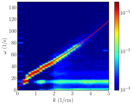
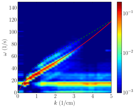
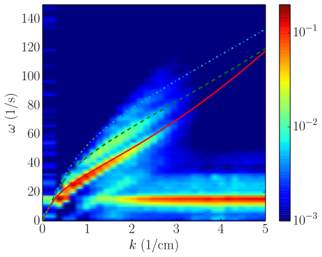
Figure 8: Spatio-temporal power spectrum of the surface deformation in CGS units for three surface wave experiments. From top to bottom, the amplitude of the forcing is respectively $1$ cm, $2$ cm, and $3$ cm. The solid line indicates the linear dispersion relation of gravity-capillary waves $\omega_{W}(k)$, the dashed line indicates the dispersion relation of 2nd-order bound waves, and the dash-dotted line indicates the dispersion relation of 3rd-order bound waves.

In Fig. 6 we show the spatio-temporal spectrum of the potential energy, $E_{\theta}(k_{x}=0,k_{y},k_{z}=10)$, for the simulation of stratified turbulence. As in the previous section, we use a flat top filter in time to compute the spectrum and reduce spectral leakage. The dispersion relation of internal gravity waves, $\omega_{S}(k)$, and two Doppler shifted branches, $\omega_{S}(k)+U_{y}k_{y}$ and $\omega_{S}(k)-U_{y}k_{y}$ are also shown as a reference (where $U_{y}=0.4$ is the horizontal r.m.s. velocity measured from the flow). Unlike the rotating case, energy is not concentrated in a narrow region around the linear dispersion relation. Instead, energy is spread within the two Doppler-shifted branches. This is the result of the presence of VSHW in the flow. In each horizontal layer the horizontal velocity takes values between $\approx\pm U_{y}$, and the frequency of the waves is shifted accordingly. Moreover, the distribution of energy in the fan defined by the two Doppler shifted dispersion relations is not uniform, as the region with $\omega<U_{y}k_{y}$ has almost negligible energy. This is the result of critical layer absorption: for $\omega<U_{y}k_{y}$, there are layers such that the phase velocity can match the horizontal wind, and waves are then absorbed.

Although there is more complexity and a larger variety of phenomena involving waves in this flow than in the rotating case, modes that can be associated with waves concentrate more energy in a wider range of scales than in the rotating flow discussed in the previous section. To illustrate this, Fig. 6 also shows the ratio of the potential energy in the fan between the two dispersion relations $\omega_{S}(k)\pm U_{y}k_{y}$, to the total potential energy at the same wavenumber. Interestingly, and except at the largest scales (smallest wavenumbers), around $70\%$ of the energy corresponds to Doppler shifted waves.

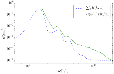
Figure 9: Frequency spectrum $E(\omega)$ from the water waves experiment, calculated directly as $\sum_{k}E(k,\omega)$) (dashed blue line), and by changing variables in the wavenumber spectrum using the dispersion relation $\omega=\omega_{W}(k)$ (solid green line). As waves provide the only relevant timescale in this system, the main features from one spectrum can be recovered from the other.

Following the same procedure as in the case of rotating turbulence, we can calculate frequency spectra from the spatio-temporal spectrum. Note however that vortical (or slow) modes in the stratified case are associated with modes with $k_{\perp}=0$, while wave (or fast) modes now are associated with modes with $k_{\perp}>0$. The resulting spectra are shown in Fig. 7. Unlike the rotating case shown in Fig. 5, now most of the energy seems to be in the $E_{w}(\omega)$ spectrum. Moreover, frequencies $\omega>2N$ now can still be associated with wave motions per virtue of the Doppler shift observed in Fig.  6.

3.4 Water waves

Water waves are the archetypical wave turbulent system, and have been studied by such theories ever since their inception (see an introduction in Nazarenko ). As a result, determining whether the energy of the system is indeed concentrated in wave modes, and what is the precise spectrum of the waves, were always major concerns for experimentalists (see, e.g., Maurel09 ; Cobelli09 and references therein). New experimental techniques, such as those described in the introduction, allowed detailed studies of free-surface deformation with spatial and temporal resolution, thus allowing direct computation of the wave energy spectrum without a priori knowledge of the dispersion relation of the system.

In Fig. 8 we show the spatio-temporal power spectrum of the fluctuations of the surface height deformation $h(x,y,t)$, as obtained from the experiment using the EMDP technique. This spectrum is proportional to the spectrum of the potential energy, and under certain conditions, proportional to the spectrum of the so-called wave action in wave turbulence theories Nazarenko . Three cases are shown under the three different forcings described above, i.e., for displacements of the wave makers respectively of $A=1$ cm, $2$ cm, and $3$ cm.

In all cases shown in Fig. 8 there is a concentration of energy around modes that satisfy the dispersion relation of gravity-capillary surface waves, $\omega_{W}(k)$, indicated in the figure by the solid line. There is also a trace of the forcing for $\omega=2\pi\times 2.7\,\textrm{s}^{-1}\approx 17\,\textrm{s}^{-1}$, with increasing power as the amplitude of the forcing is increased. Also, as the forcing increases, new modes that do not satisfy any of these relations are excited.

Indeed, for larger forcing amplitudes two features can be identified. On the one hand, the width (in terms of the wavenumber) of the dispersion relation $\omega_{W}(k)$ decreases: while for forcing amplitude of $1$ cm gravity-capillary waves can be identified up to $k\approx 4$ cm^-1, for forcing amplitude of $3$ cm the dispersion relation extends up to $k\approx 3$ cm^-1. On the other hand, new wave branches are excited. These correspond to bound waves Longuet63 ; Herbert10 . Bound waves are small amplitude waves that travel in front of (i.e., they have the same phase velocity as) a larger amplitude parent wave. They can be generated by the breaking of the longer waves, by nonlinear distortion of the parent wave, or be parasitic capillaries travelling on the front of the parent wave. As they travel on the front of the long wave, they are phase-locked, and as they have the same phase velocity, their dispersion relation is given by Longuet63 ; Herbert10

$$\Omega_{N}(Nk)=N\omega_{W}(k),$$

where $N$ is the order of the bounded waves. The dotted and dash-dotted lines in Fig. 8 indicate the dispersion relation of bound waves for $N=2$ and $3$. The shortening of the width of the dispersion relation $\omega_{W}(k)$, together with the excitation of higher order bound waves as the forcing amplitude is increased, indicates that with larger amplitudes the energy transfer mechanism shifts from a cascade to gravity-capillary waves with smaller wavenumbers, to a transfer of energy towards higher-order bound waves with smaller frequencies.

For one of the experiments (the case with displacement of the wavemakers of 1 cm), we show in Fig. 9 the frequency spectrum $E(\omega)$ calculated as $\sum_{k}E(k,\omega)$, and the spectrum computed from the spatial spectrum $E(k)$ using the dispersion relation to change variables to obtain $E(k(\omega))dk/d\omega$. Although the agreement is not as good as in the case of isotropic and homogeneous turbulence (Fig. 3), the main features of one spectrum can be recovered from the other. This suggests that the dominant time scale in the system is given by the period of the waves, unlike the previous cases where multiple time scales could be identified at a given wavenumber.

4 Conclusions

We presented four examples of turbulent flows where the spatio-temporal spectrum can be used to identify key flow features and reveal aspects of their dynamics. The examples considered are numerical simulations of isotropic and homogeneous turbulence, of rotating turbulence, and of stratified turbulence, and laboratory experiments of gravity-capillary water wave turbulence. Two of these cases were reported extensively in Clark14a ; Clark15 , while the results for the cases of isotropic and homogeneous turbulence and of water wave turbulence are new.

In all these cases, the spatio-temporal spectrum allows quantification of the energy in wave motions, in bound waves, and in eddies, as well as identification of physical effects such as sweeping, Doppler shift, and critical layer absorption. For isotropic and homogeneous turbulence, the dominant Eulerian timescale is sweeping, as expected from previous studies considering decorrelation times Chen89 ; Nelkin90 ; Sanada92 . For rotating turbulence, the dominant timescale at intermediate scales is the period of inertial waves, although the energy in inertial waves drops to less than $\approx 10\%$ for scales which are still much larger than the Zeman scale for which eddies are expected to be as important as the waves. The case of stratified turbulence is much more complex, with the spatio-temporal spectrum showing Doppler shift of internal gravity waves by the horizontal winds, and absorption of waves in critical layers where the wave speed matches the horizontal wind speed. Finally, in the laboratory experiments of water wave turbulence, the spectrum shows evidence of the presence of bound waves, as reported before in Longuet63 ; Herbert10 . A study varying the forcing indicates that as the forcing amplitude is increased, the energy transfer mechanism shifts from a cascade to gravity-capillary waves with smaller wavenumbers, to a transfer of energy towards higher-order bound waves with smaller frequencies.

References

- [1] A. Celani B. J. Devenish A. Lanotte L. Biferale, G. Boffetta and F. Toschi. Multifractal statistics of lagrangian velocity and acceleration in turbulence. Phys. Rev. Lett., 93:064502, Aug 2004.
- [2] A. K. M. Fazle Hussain. Coherent structures and turbulence. J. Fluid Mech., 173:303–356, December 1986.
- [3] M. M. Rogers and P. Moin. The structure of the vorticity field in homogeneous turbulent flows. J. Fluid Mech., 176:33–66, 1987.
- [4] P. Holmes G. Berkooz and J. L. Lumley. The Proper Orthogonal Decomposition in the Analysis of Turbulent Flows. Annual Review of Fluid Mechanics, 25(1):539–575, 1993.
- [5] J. Moehlis T. R. Smith and P. Holmes. Low-dimensional modelling of turbulence using the proper orthogonal decomposition: a tutorial. Nonlinear Dynamics, 41(1-3):275–307, 2005.
- [6] J. D. Woods. Do waves limit turbulent diffusion in the ocean? Nature, 288:219–224, November 1980.
- [7] C. Cambon and L. Jacquin. Spectral approach to non-isotropic turbulence subjected to rotation. J. Fluid Mech., 202:295–317, 1989.
- [8] F. Waleffe. Inertial transfers in the helical decomposition. Phys. Fluids A, 5(3):677, 1993.
- [9] C. Cambon, N. N. Mansour, and F. S. Godeferd. Energy transfer in rotating turbulence. J. Fluid Mech., 337:303–332, 1997.
- [10] Sergey Nazarenko. Wave Turbulence. Springer, 2011 edition, February 2011.
- [11] R. W. Stewart. Turbulence and Waves in a Stratified Atmosphere. Radio Science, 4:1269–1278, December 1969.
- [12] L. M. Smith and F. Waleffe. Generation of slow large scales in forced rotating stratified turbulence. J. Fluid Mech., 451:145–168, January 2002.
- [13] L. Bourouiba. Model of a truncated fast rotating flow at infinite reynolds number. Phys. Fluids, 20(7):–, 2008.
- [14] D. Rosenberg A. Sen, P. D. Mininni and A. Pouquet. Anisotropy and nonuniversality in scaling laws of the large-scale energy spectrum in rotating turbulence. Phys. Rev. E, 86:036319, Sep 2012.
- [15] R. J. Adrian. Particle-imaging techniques for experimental fluid mechanics. Annual review of fluid mechanics, 23(1):261–304, 1991.
- [16] V. Pagneux A. Maurel, P. Cobelli and P. Petitjeans. Experimental and theoretical inspection of the phase-to-height relation in Fourier transform profilometry. Applied Optics, 48(2):380–392, January 2009.
- [17] A. Maurel V. Pagneux P. Cobelli, P. Petitjeans and N. Mordant. Space-Time Resolved Wave Turbulence in a Vibrating Plate. Phys. Rev. Lett., 103(20):204301, November 2009.
- [18] G. Lagubeau, P. Cobelli, T. Bobinski, A. Maurel, V. Pagneux, and P. Petitjeans. Empirical mode decomposition profilometry: small-scale capabilities and comparison to fourier transform profilometry. Appl. Opt., 54(32):9409–9414, Nov 2015.
- [19] P. Carns C. Carothers R. Ross G. Grider A. Crume N. Liu, J. Cope and C. Maltzahn. On the role of burst buffers in leadership-class storage systems. In Mass Storage Systems and Technologies (MSST), 2012 IEEE 28th Symposium on, pages 1–11. IEEE, 2012.
- [20] F. Moisy A. Campagne, B. Gallet and P.-P. Cortet. Disentangling inertial waves from eddy turbulence in a forced rotating turbulence experiment. Phys. Rev. E, April 2015.
- [21] Gregory P. Bewley, Daniel P. Lathrop, Leo R. M. Maas, and K. R. Sreenivasan. Inertial waves in rotating grid turbulence. Phys. Fluids, 19(7):071701, July 2007.
- [22] D. S. Zimmerman M. Rieutord, S. A. Triana and D. P. Lathrop. Excitation of inertial modes in an experimental spherical Couette flow. Phys. Rev. E, 86(2):026304, August 2012.
- [23] Cyril Lamriben, Pierre-Philippe Cortet, Frédéric Moisy, and Leo R. M. Maas. Excitation of inertial modes in a closed grid turbulence experiment under rotation. Phys. Fluids, 23(1):015102, January 2011.
- [24] P. Dmitruk S. Servidio, V. Carbone and W. H. Matthaeus. Time decorrelation in isotropic magnetohydrodynamic turbulence. Europhys. Lett., 96(5):55003, December 2011.
- [25] F. S. Godeferd B. Favier and C. Cambon. On space and time correlations of isotropic and rotating turbulence. Phys. Fluids, 22(1):015101, 2010.
- [26] P. D. Mininni P. Dmitruk P. Clark di Leoni, P. J. Cobelli and W. H. Matthaeus. Quantification of the strength of inertial waves in a rotating turbulent flow. Phys. Fluids, 26(3):035106, March 2014.
- [27] P. Dmitruk and W. H. Matthaeus. Waves and turbulence in magnetohydrodynamic direct numerical simulations. Phys. Plasmas, 16(6):062304, June 2009.
- [28] E. Lindborg and G. Brethouwer. Stratified turbulence forced in rotational and divergent modes. J. Fluid Mech., 586:83–108, September 2007.
- [29] E. A. D’Asaro and R.-C. Lien. Lagrangian Measurements of Waves and Turbulence in Stratified Flows. Journal of Physical Oceanography, 30(3):641–655, March 2000.
- [30] P. Cobelli, A. Przadka, P. Petitjeans, G. Lagubeau, V. Pagneux, and A. Maurel. Different Regimes for Water Wave Turbulence. Phys. Rev. Lett., 107(21):214503, November 2011.
- [31] Quentin Aubourg and Nicolas Mordant. Nonlocal Resonances in Weak Turbulence of Gravity-Capillary Waves. Phys. Rev. Lett., 114:144501, April 2015.
- [32] P. D. Mininni P. Clark di Leoni, P. J. Cobelli. Wave turbulence in shallow water models. Phys. Rev. E, 89(6):063025, June 2014.
- [33] Naoto Yokoyama and Masanori Takaoka. Identification of a separation wave number between weak and strong turbulence spectra for a vibrating plate. Phys. Rev. E, 89(1):012909, January 2014.
- [34] E. Yarom and E. Sharon. Experimental observation of steady inertial wave turbulence in deep rotating flows. Nature Physics, 10(7):510–514, June 2014.
- [35] R. Meyrand, K. H. Kiyani, and S. Galtier. Weak magnetohydrodynamic turbulence and intermittency. J. Fluid Mech., 770, May 2015.
- [36] P. Clark di Leoni and P. D. Mininni. Absorption of waves by large-scale winds in stratified turbulence. Phys. Rev. E, 91(3):033015, March 2015.
- [37] Sergey Nazarenko and Miguel Onorato. Wave turbulence and vortices in Bose–Einstein condensation. Physica D: Nonlinear Phenomena, 219(1):1–12, July 2006.
- [38] Sergey Nazarenko and Miguel Onorato. Freely decaying Turbulence and Bose–Einstein Condensation in Gross–Pitaevski Model. Journal of Low Temperature Physics, 146(1-2):31–46, January 2007.
- [39] Patricio Clark di Leoni, Pablo D. Mininni, and Marc E. Brachet. Direct evidence of Kelvin waves in numerical simulations of quantum turbulence. arXiv:1509.05316 [physics], September 2015. arXiv: 1509.05316.
- [40] M. L. Goldstein F. Sahraoui, G. Belmont and L. Rezeau. Limitations of multispacecraft data techniques in measuring wave number spectra of space plasma turbulence. Journal of Geophysical Research, 115(A4):A04206–10, April 2010.
- [41] G. Belmont A. Roux L. Rezeau P. Canu P. Robert N. Cornilleau-Wehrlin O. Le Contel T. D. De Wit J.-L. Pinçon F. Sahraoui, M. L. Goldstein and K. Kiyani. Multi-spacecraft investigation of space turbulence Lessons from Cluster and input to the Cross-Scale mission. Planetary and Space Science, 59(7):585–591, May 2011.
- [42] C.P. Escoubet, R. Schmidt, and C. Russell. The Cluster and Phoenix Missions. Space science reviews. Springer Netherlands, 1997.
- [43] S. Tomczyk R. J. Morton and R. Pinto. Investigating Alfvénic wave propagation in coronal open-field regions. Nature Comm., 6, 2015.
- [44] P. D. Mininni D. Gómez and P. Dmitruk. MHD simulations and astrophysical applications. Advances in Space Research, 35(5):899–907, 2005.
- [45] P. D. Mininni D. Gómez and P. Dmitruk. Parallel simulations in turbulent MHD. Phys. Scripta, 2005:123, 2005.
- [46] R. Reddy P. Mininni, D. Rosenberg and A. Pouquet. A hybrid MPI-OpenMP scheme for scalable parallel pseudospectral computations for fluid turbulence. Parallel Computing, 37(6-7):316–326, 2011.
- [47] A. Przadka, B. Cabane, V. Pagneux, A. Maurel, and P. Petitjeans. Fourier transform profilometry for water waves: how to achieve clean water attenuation with diffusive reflection at the water surface? Exp. Fluids, 52(2):519–527, 2012.
- [48] P. A. Davidson. Turbulence: an introduction for scientists and engineers. Oxford Univ. Press, Oxford, 2004.
- [49] H. Tennekes. Eulerian and Lagrangian time microscales in isotropic turbulence. J. Fluid Mech., 67(3):561–567, 1975.
- [50] S. Chen and R. H. Kraichnan. Sweeping decorrelation in isotropic turbulence. Phys. Fluids A, 1(12):2019, December 1989.
- [51] M. Nelkin and M. Tabor. Time correlations and random sweeping in isotropic turbulence. Phys. Fluids A, 2(1):81–83, January 1990.
- [52] T. Sanada and V. Shanmugasundaram. Random sweeping effect in isotropic numerical turbulence. Phys. Fluids A, 4(6):1245–1250, June 1992.
- [53] D. Rosenberg P. D. Mininni and A. Pouquet. Isotropization at small scales of rotating helically driven turbulence. J. Fluid Mech., 699:263–279, 2012.
- [54] A. C. Newell. Rossby wave packet interactions. J. Fluid Mech., 35(02):255–271, January 1969.
- [55] C. Cambon, R. Rubinstein, and F. S. Godeferd. Advances in wave turbulence: rapidly rotating flows. New J. Phys., 6:73, 2004.
- [56] A. Alexakis. Rotating taylor–green flow. J. Fluid Mech., 769:46–78, 2015.
- [57] D. Rosenberg R. Marino, P. D. Mininni and A. Pouquet. Inverse cascades in rotating stratified turbulence: Fast growth of large scales. Europhys. Lett., 102(4):44006, 2013.
- [58] A. Pouquet C. Herbert and R. Marino. Restricted equilibrium and the energy cascade in rotating and stratified flows. J. Fluid Mech., 758:374–406, November 2014.
- [59] C. O. Hines. The saturation of gravity waves in the middle atmosphere. part II: development of doppler-spread theory. J. Atmos. Sci., 48(11):1361–1379, June 1991.
- [60] K. B. Winters and E. A. D’Asaro. Three-dimensional wave instability near a critical level. J. Fluid Mech., 272:255–284, August 1994.
- [61] M. S. Longuet-Higgins. The generation of capillary waves by steep gravity waves. J. Fluid Mech., 16(01):138–159, 1963.
- [62] N. Mordant E. Herbert and E. Falcon. Observation of the Nonlinear Dispersion Relation and Spatial Statistics of Wave Turbulence on the Surface of a Fluid. Phys. Rev. Lett., 105(14):144502, September 2010.